A Simple Tutorial on Theano

Jiang Guo

Outline

• What’s Theano?

• How to use Theano?

– Basic Usage: How to write a theano program

– Advanced Usage: Manipulating symbolic expressions

• Case study 1: Logistic Regression

• Case study 2: Multi-layer Perceptron

• Case study 3: Recurrent Neural Network

WHAT’S THEANO?

Theano is many things

• Programming Language

• Linear Algebra Compiler

• Python library – Define, optimize, and evaluate mathematical

expressions involving multi-dimensional arrays.

• Note: Theano is not a machine learning toolkit, but a mathematical toolkit that makes building downstream machine learning models easier. – Pylearn2

Theano features

• Tight integration with NumPy

• Transparent use of a GPU

• Efficient symbolic differentiation

• Speed and stability optimizations

• Dynamic C code generation

Project Status

• Theano has been developed and used since 2008, by LISA lab at the University of Montreal (leaded by Yoshua Bengio) – Citation: 202 (LTP: 88)

• Deep Learning Tutorials

• Machine learning library built upon Theano – Pylearn2

• Good user documentation – http://deeplearning.net/software/theano/

• Open-source on Github

HOW TO USE THEANO? Basic Usage

Python in 1 Slide

• Interpreted language

• OO and scripting language

• Emphasizes code readability

• Large and comprehensive standard library

• Indentation for block delimiters

• Dynamic type

• Dictionary – d={‘key1’:‘val1’, ‘key2’:42, …}

• List comprehension – [i+3 for i in range(10)]

NumPy in 1 Slide

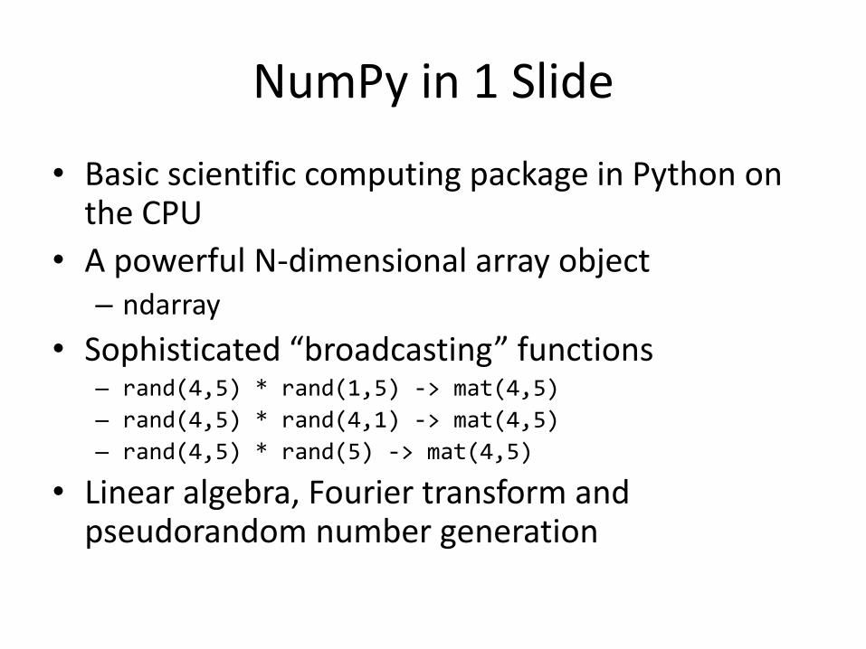
• Basic scientific computing package in Python on the CPU

• A powerful N-dimensional array object – ndarray

• Sophisticated “broadcasting” functions – rand(4,5) * rand(1,5) -> mat(4,5)

– rand(4,5) * rand(4,1) -> mat(4,5)

– rand(4,5) * rand(5) -> mat(4,5)

• Linear algebra, Fourier transform and pseudorandom number generation

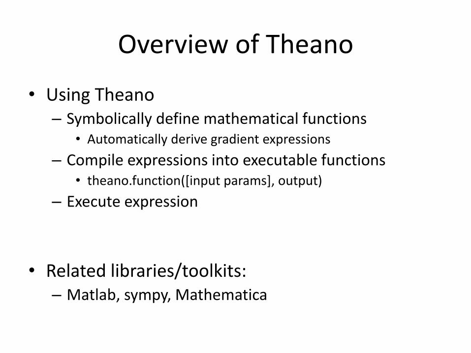
Overview of Theano

• Using Theano – Symbolically define mathematical functions

• Automatically derive gradient expressions

– Compile expressions into executable functions • theano.function([input params], output)

– Execute expression

• Related libraries/toolkits: – Matlab, sympy, Mathematica

Installing Theano

• Requirements

– OS: Linux, Mac OS X, Windows

– Python: >= 2.6

– Numpy, Scipy, BLAS

• pip install [--upgrade] theano

• easy_install [--upgrade] theano

• Install from source code

– https://github.com/Theano/Theano

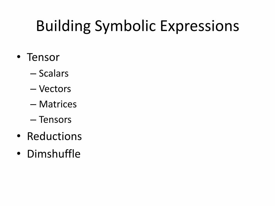
Building Symbolic Expressions

• Tensor

– Scalars

– Vectors

– Matrices

– Tensors

• Reductions

• Dimshuffle

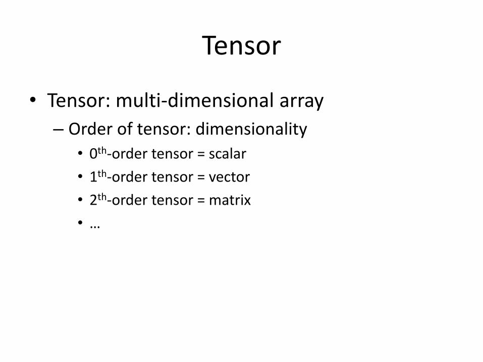
Tensor

• Tensor: multi-dimensional array

– Order of tensor: dimensionality

• 0th-order tensor = scalar

• 1th-order tensor = vector

• 2th-order tensor = matrix

• …

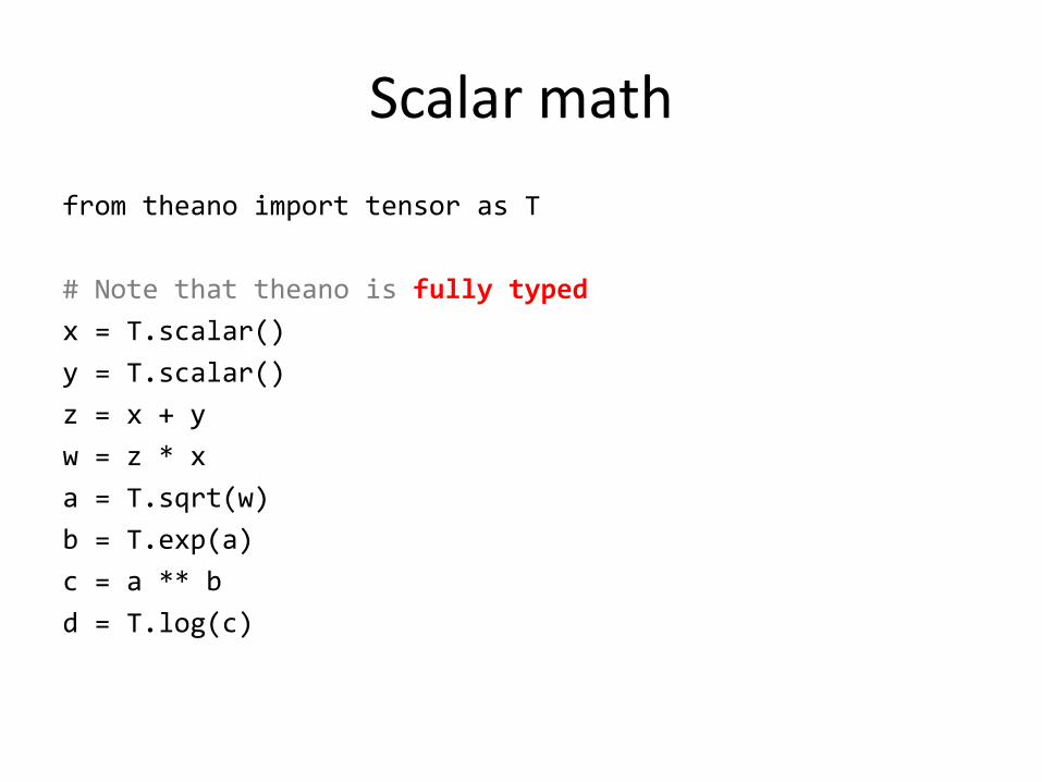
Scalar math

from theano import tensor as T

# Note that theano is fully typed

x = T.scalar()

y = T.scalar()

z = x + y

w = z * x

a = T.sqrt(w)

b = T.exp(a)

c = a ** b

d = T.log(c)

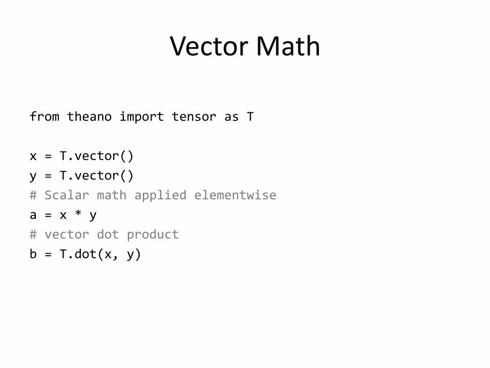
Vector Math

from theano import tensor as T

x = T.vector()

y = T.vector()

# Scalar math applied elementwise

a = x * y

# vector dot product

b = T.dot(x, y)

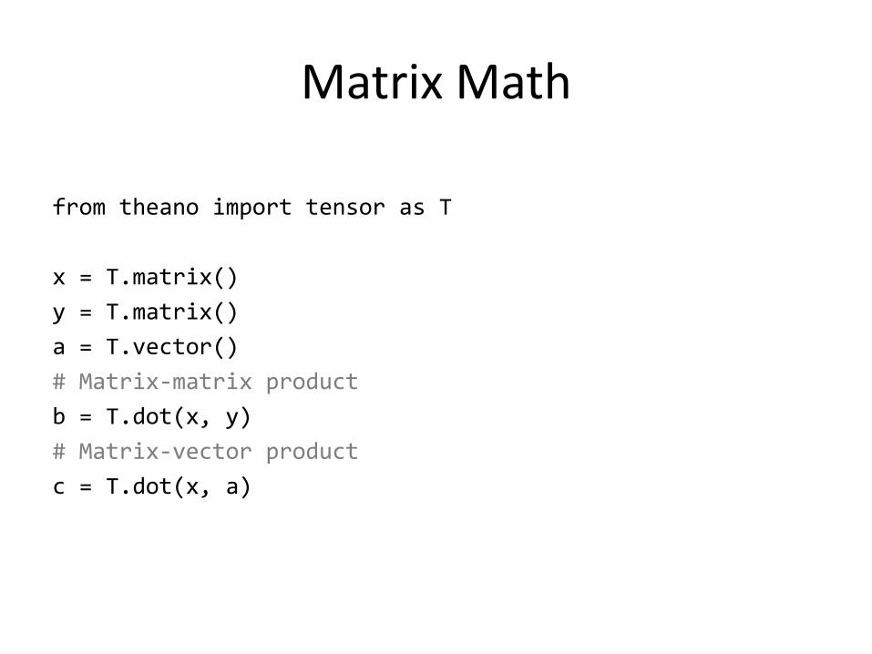
Matrix Math

from theano import tensor as T

x = T.matrix()

y = T.matrix()

a = T.vector()

# Matrix-matrix product

b = T.dot(x, y)

# Matrix-vector product

c = T.dot(x, a)

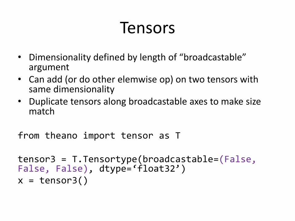
Tensors

• Dimensionality defined by length of “broadcastable” argument

• Can add (or do other elemwise op) on two tensors with same dimensionality

• Duplicate tensors along broadcastable axes to make size match

from theano import tensor as T tensor3 = T.Tensortype(broadcastable=(False, False, False), dtype=‘float32’) x = tensor3()

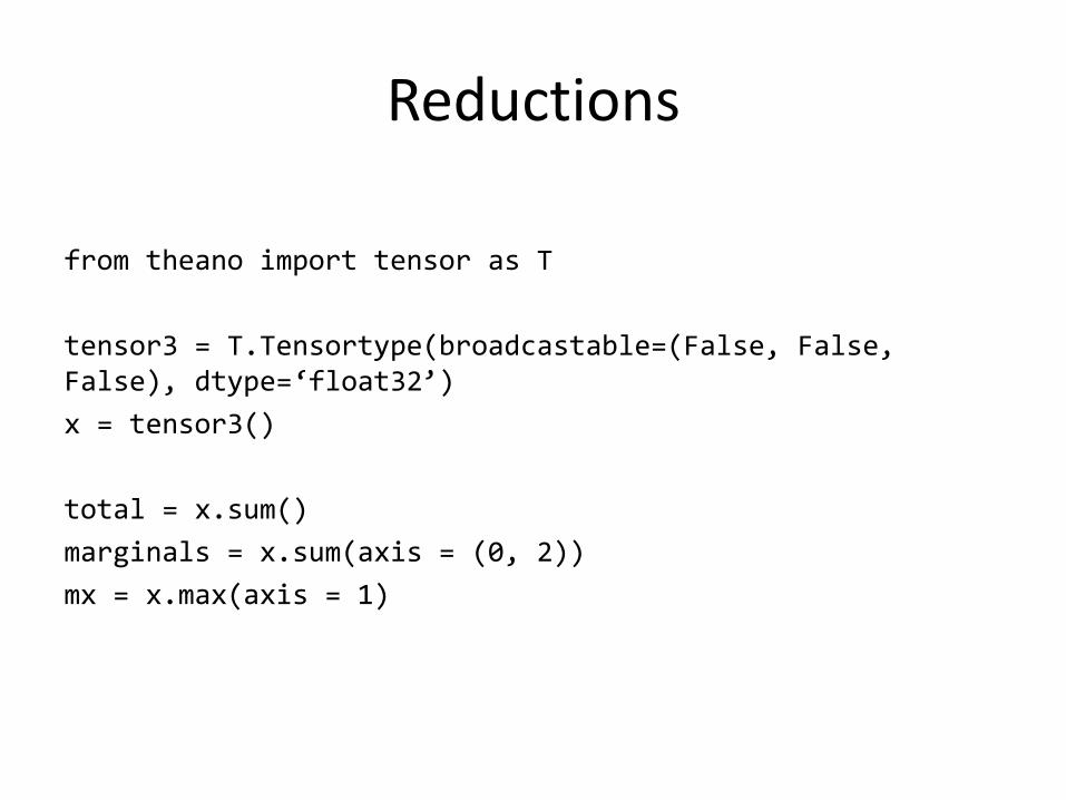
Reductions

from theano import tensor as T

tensor3 = T.Tensortype(broadcastable=(False, False, False), dtype=‘float32’)

x = tensor3()

total = x.sum()

marginals = x.sum(axis = (0, 2))

mx = x.max(axis = 1)

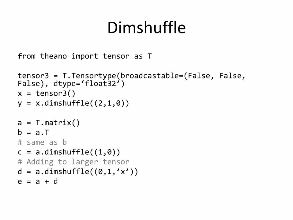
Dimshuffle

from theano import tensor as T tensor3 = T.Tensortype(broadcastable=(False, False, False), dtype=‘float32’) x = tensor3() y = x.dimshuffle((2,1,0)) a = T.matrix() b = a.T # same as b c = a.dimshuffle((1,0)) # Adding to larger tensor d = a.dimshuffle((0,1,’x’)) e = a + d

zeros_like and ones_like

• zeros_like(x) returns a symbolic tensor with the same shape and dtype as x, but with every element to 0

• ones_like(x) is the same thing, but with 1s

Compiling and running expressions

• theano.function

• shared variables and updates

• compilation modes

• compilation for GPU

• optimizations

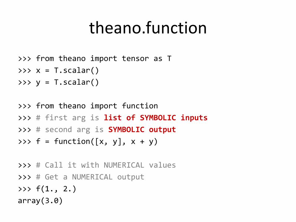
theano.function

>>> from theano import tensor as T

>>> x = T.scalar()

>>> y = T.scalar()

>>> from theano import function

>>> # first arg is list of SYMBOLIC inputs

>>> # second arg is SYMBOLIC output

>>> f = function([x, y], x + y)

>>> # Call it with NUMERICAL values

>>> # Get a NUMERICAL output

>>> f(1., 2.)

array(3.0)

Shared variables

• A “shared variable” is a buffer that stores a numerical value for a theano variable

– think as a global variable

• Modify outside function with get_value and set_value

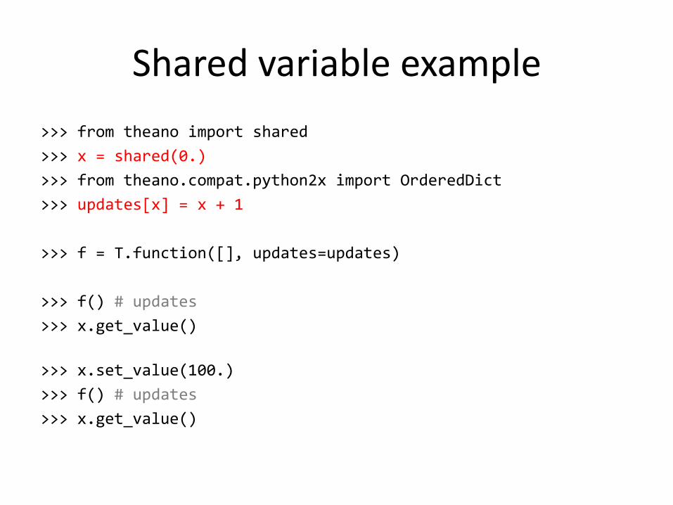
Shared variable example

>>> from theano import shared

>>> x = shared(0.)

>>> from theano.compat.python2x import OrderedDict

>>> updates[x] = x + 1

>>> f = T.function([], updates=updates)

>>> f() # updates

>>> x.get_value()

>>> x.set_value(100.)

>>> f() # updates

>>> x.get_value()

Compilation modes

• Can compile in different modes to get different kinds of programs

• Can specify these modes very precisely with arguments to theano.function

• Can use a few quick presets with environment variable flags

Example preset compilation modes

• FAST_RUN

• FAST_COMPILE

• DEBUG_MODE

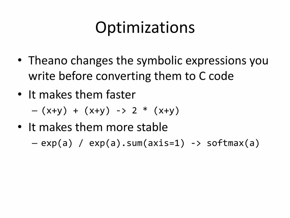
Optimizations

• Theano changes the symbolic expressions you write before converting them to C code

• It makes them faster – (x+y) + (x+y) -> 2 * (x+y)

• It makes them more stable – exp(a) / exp(a).sum(axis=1) -> softmax(a)

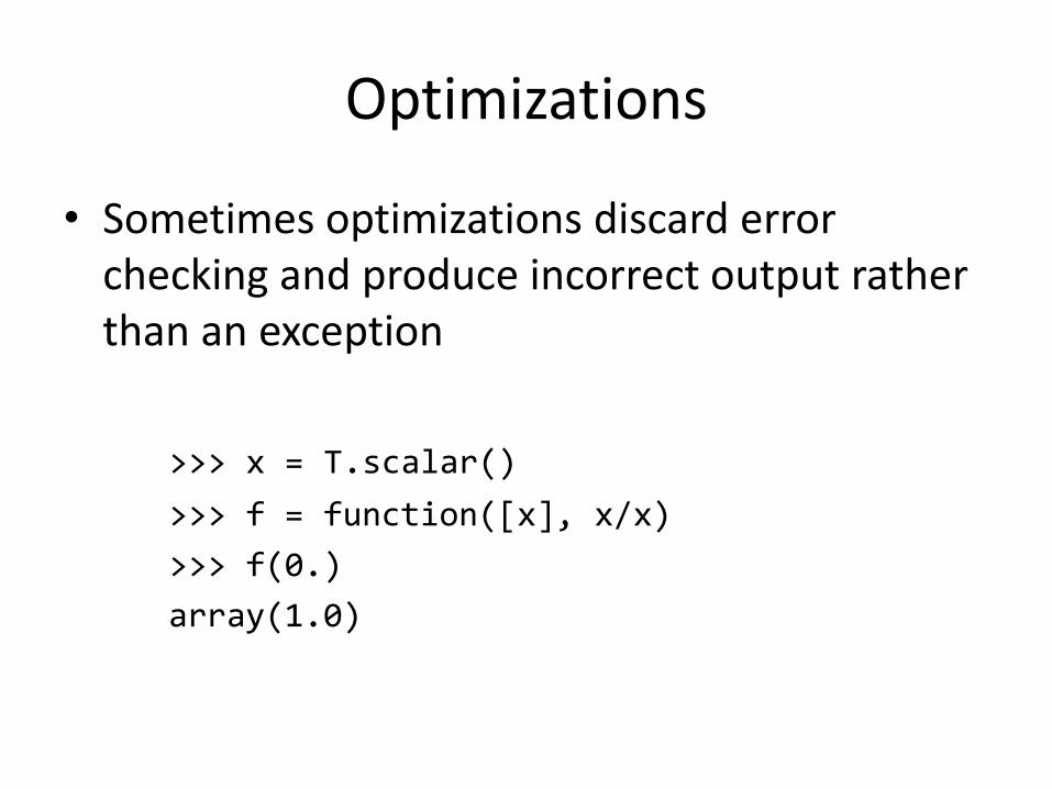
Optimizations

• Sometimes optimizations discard error checking and produce incorrect output rather than an exception

>>> x = T.scalar()

>>> f = function([x], x/x)

>>> f(0.)

array(1.0)

HOW TO USE THEANO? Advanced Usage

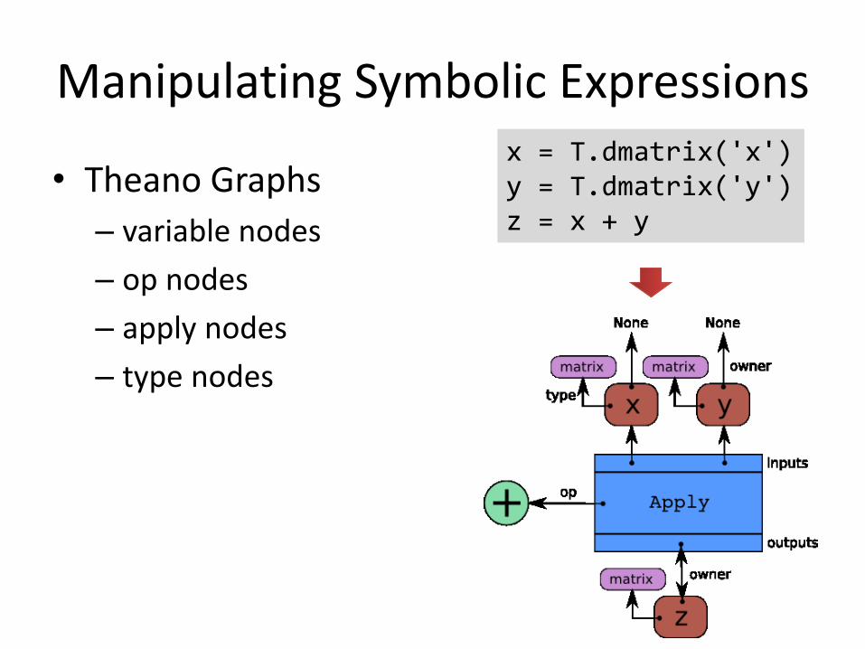
Manipulating Symbolic Expressions

• Theano Graphs

– variable nodes

– op nodes

– apply nodes

– type nodes

x = T.dmatrix('x') y = T.dmatrix('y') z = x + y

Manipulating Symbolic Expressions

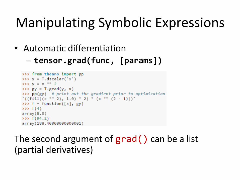
• Automatic differentiation – tensor.grad(func, [params])

The second argument of grad() can be a list (partial derivatives)

Loop: scan

• reduce and map are special cases of scan

– scan a function along some input sequence, producing an output at each time-step.

– Number of iterations is part of the symbolic graph

– Slightly faster than using a for loop with a compiled Theano function

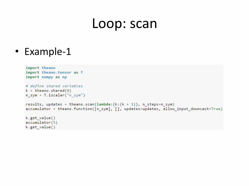
Loop: scan

• Example-1

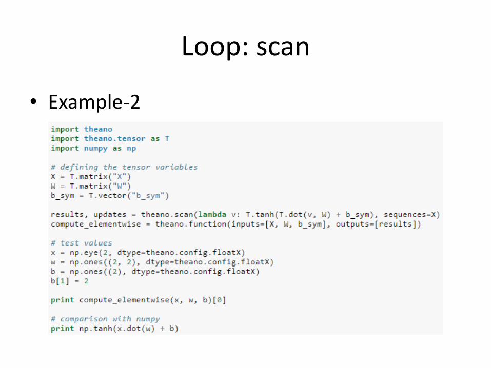
Loop: scan

• Example-2

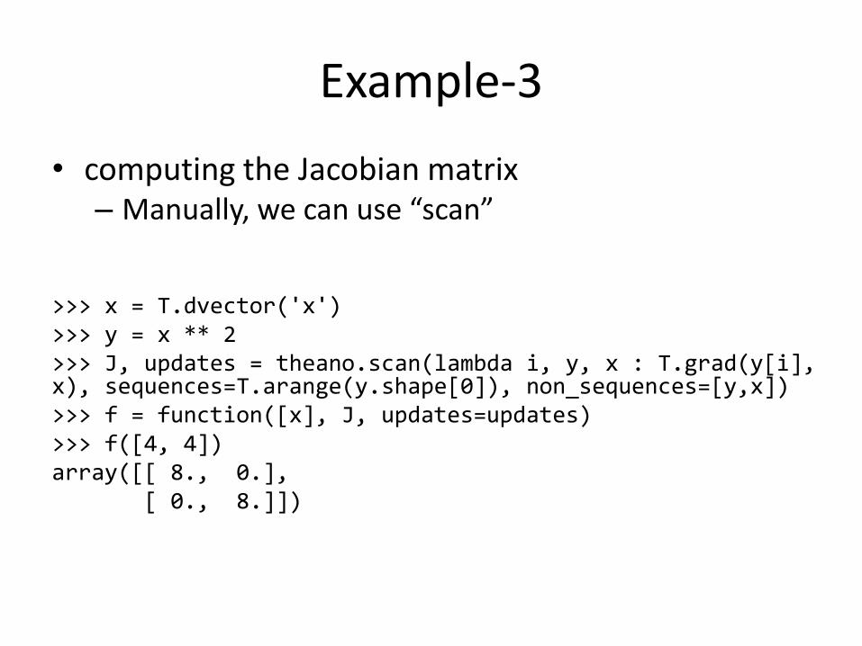
Example-3

• computing the Jacobian matrix – Manually, we can use “scan”

>>> x = T.dvector('x') >>> y = x ** 2 >>> J, updates = theano.scan(lambda i, y, x : T.grad(y[i], x), sequences=T.arange(y.shape[0]), non_sequences=[y,x]) >>> f = function([x], J, updates=updates) >>> f([4, 4]) array([[ 8., 0.], [ 0., 8.]])

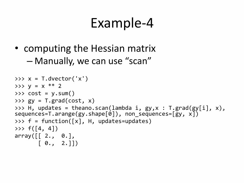
Example-4

• computing the Hessian matrix – Manually, we can use “scan”

>>> x = T.dvector('x') >>> y = x ** 2 >>> cost = y.sum() >>> gy = T.grad(cost, x) >>> H, updates = theano.scan(lambda i, gy,x : T.grad(gy[i], x), sequences=T.arange(gy.shape[0]), non_sequences=[gy, x]) >>> f = function([x], H, updates=updates) >>> f([4, 4]) array([[ 2., 0.], [ 0., 2.]])

CASE STUDY - 1 Logistic Regression

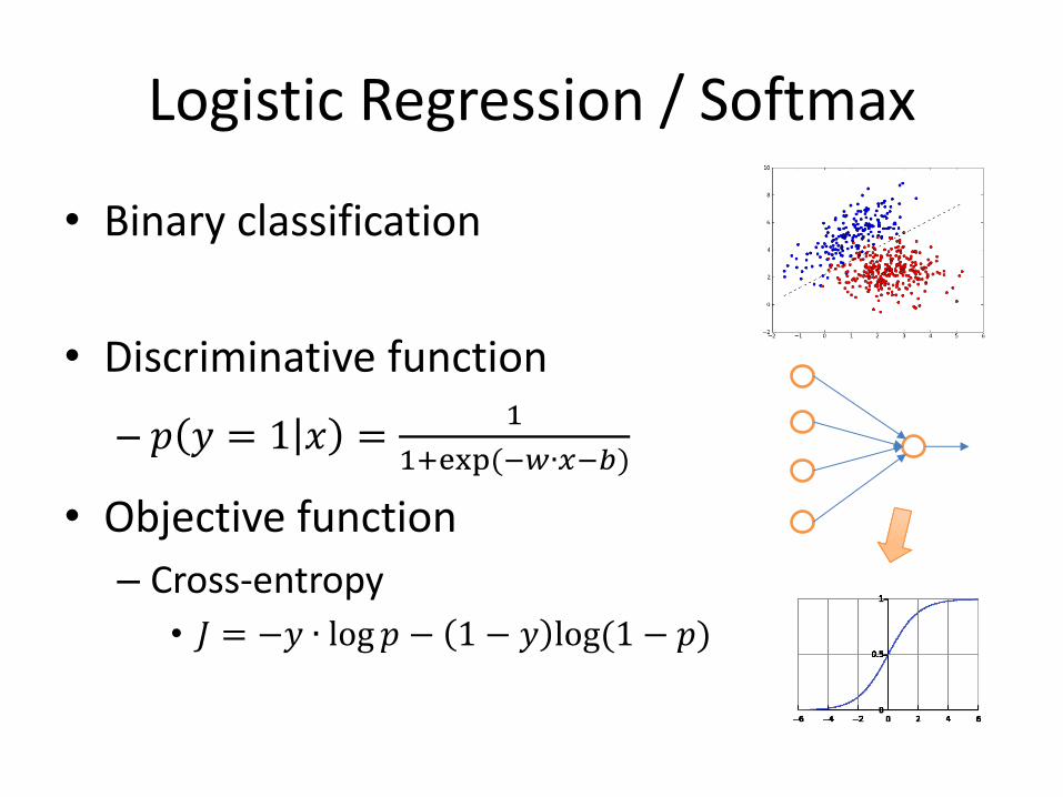
Logistic Regression / Softmax

• Binary classification

• Discriminative function

– 𝑝 𝑦 = 1 𝑥 =1

1+exp(−𝑤∙𝑥−𝑏)

• Objective function

– Cross-entropy

• 𝐽 = −𝑦 ∙ log 𝑝 − 1 − 𝑦 log(1 − 𝑝)

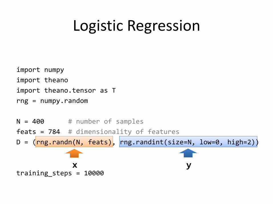
Logistic Regression

import numpy

import theano

import theano.tensor as T

rng = numpy.random

N = 400 # number of samples

feats = 784 # dimensionality of features

D = (rng.randn(N, feats), rng.randint(size=N, low=0, high=2))

training_steps = 10000 x y

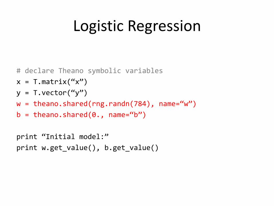
Logistic Regression

# declare Theano symbolic variables

x = T.matrix(“x”)

y = T.vector(“y”)

w = theano.shared(rng.randn(784), name=“w”)

b = theano.shared(0., name=“b”)

print “Initial model:”

print w.get_value(), b.get_value()

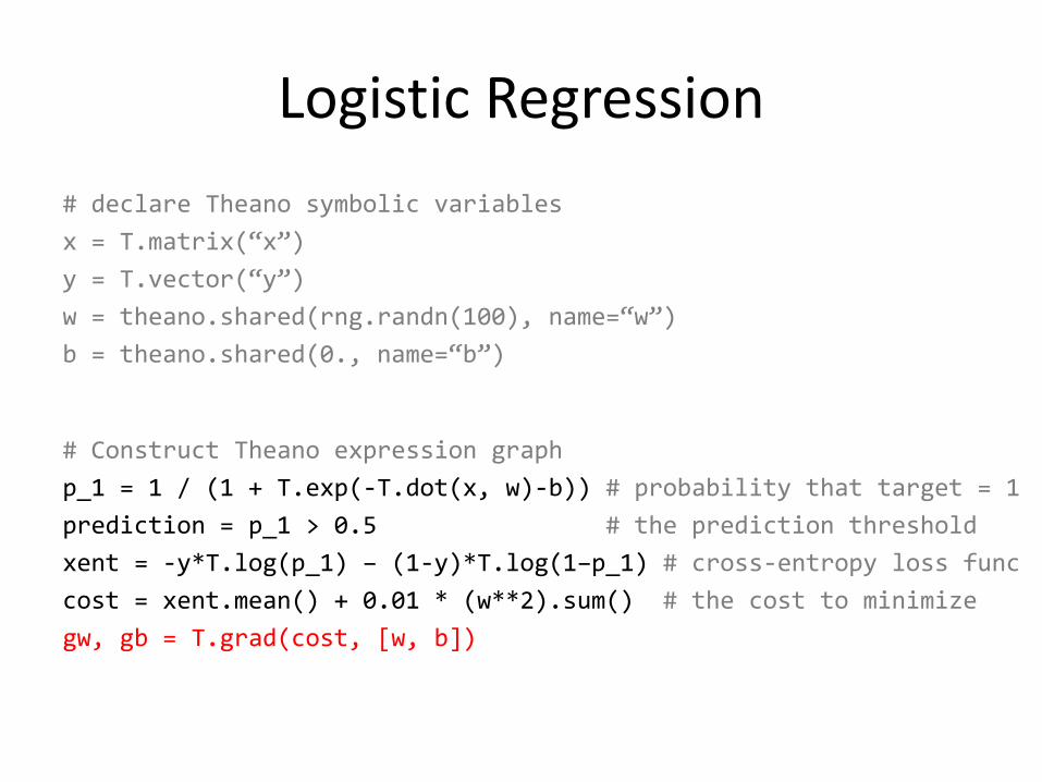
Logistic Regression

# declare Theano symbolic variables

x = T.matrix(“x”)

y = T.vector(“y”)

w = theano.shared(rng.randn(100), name=“w”)

b = theano.shared(0., name=“b”)

# Construct Theano expression graph

p_1 = 1 / (1 + T.exp(-T.dot(x, w)-b)) # probability that target = 1

prediction = p_1 > 0.5 # the prediction threshold

xent = -y*T.log(p_1) – (1-y)*T.log(1–p_1) # cross-entropy loss func

cost = xent.mean() + 0.01 * (w**2).sum() # the cost to minimize

gw, gb = T.grad(cost, [w, b])

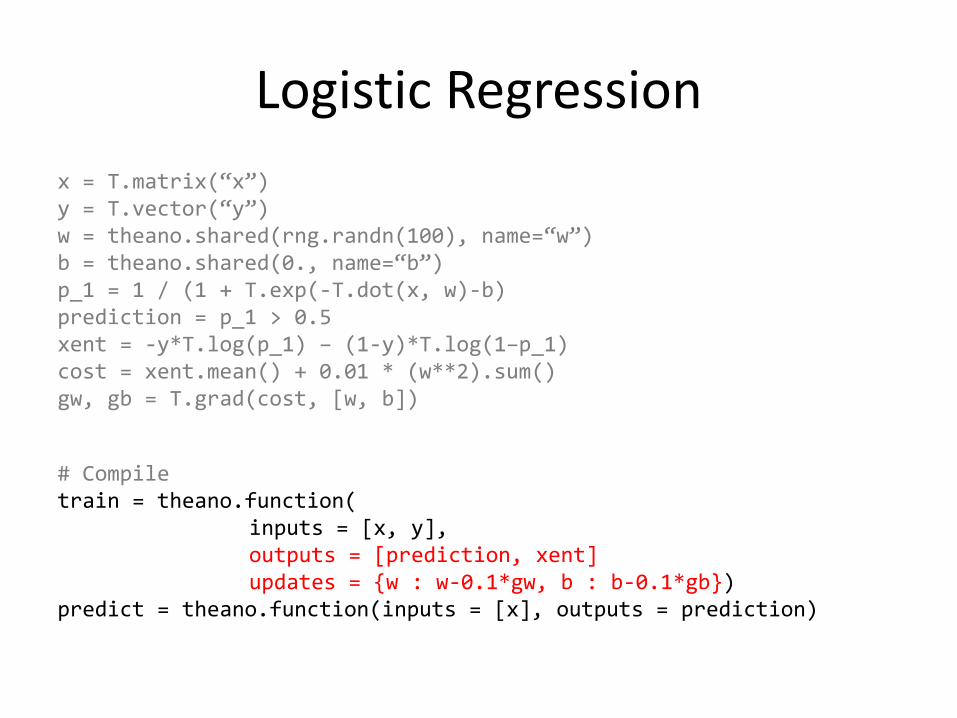
Logistic Regression

x = T.matrix(“x”) y = T.vector(“y”) w = theano.shared(rng.randn(100), name=“w”) b = theano.shared(0., name=“b”) p_1 = 1 / (1 + T.exp(-T.dot(x, w)-b) prediction = p_1 > 0.5 xent = -y*T.log(p_1) – (1-y)*T.log(1–p_1) cost = xent.mean() + 0.01 * (w**2).sum() gw, gb = T.grad(cost, [w, b])

# Compile train = theano.function( inputs = [x, y], outputs = [prediction, xent] updates = {w : w-0.1*gw, b : b-0.1*gb}) predict = theano.function(inputs = [x], outputs = prediction)

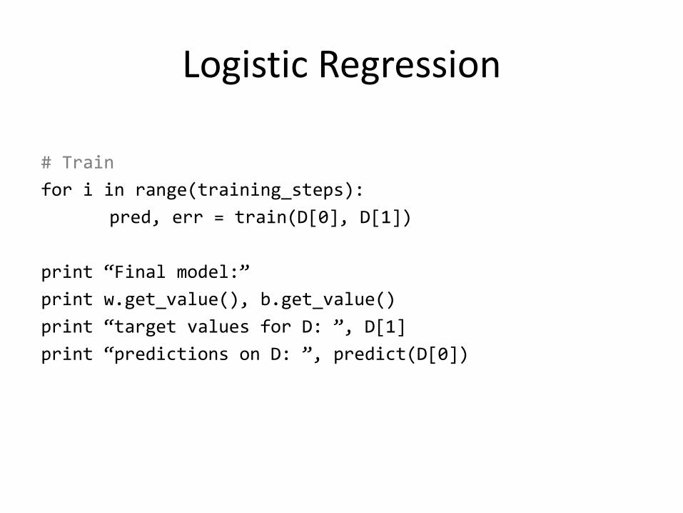
Logistic Regression

# Train

for i in range(training_steps):

pred, err = train(D[0], D[1])

print “Final model:”

print w.get_value(), b.get_value()

print “target values for D: ”, D[1]

print “predictions on D: ”, predict(D[0])

CASE STUDY - 2 Multi-Layer Perceptron

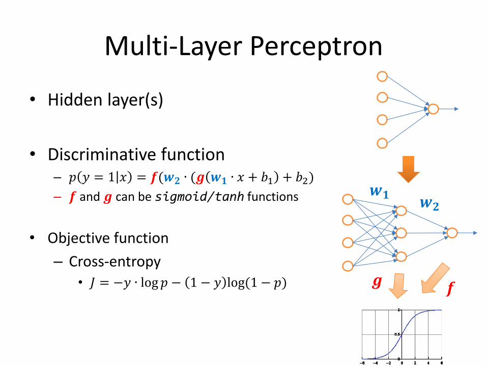
Multi-Layer Perceptron

• Hidden layer(s)

• Discriminative function – 𝑝 𝑦 = 1 𝑥 = 𝒇(𝒘𝟐 ∙ (𝒈 𝒘𝟏 ∙ 𝑥 + 𝑏1 + 𝑏2)

– 𝒇 and 𝒈 can be sigmoid/tanh functions

• Objective function

– Cross-entropy • 𝐽 = −𝑦 ∙ log 𝑝 − 1 − 𝑦 log(1 − 𝑝)

𝒇 𝒈

𝒘𝟏 𝒘𝟐

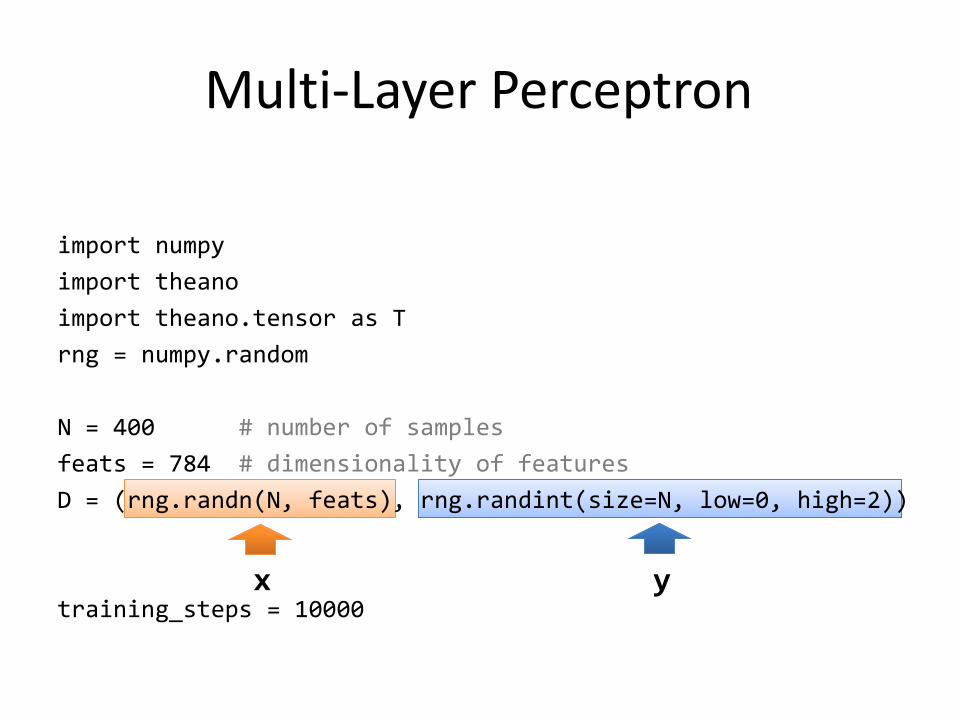
Multi-Layer Perceptron

import numpy

import theano

import theano.tensor as T

rng = numpy.random

N = 400 # number of samples

feats = 784 # dimensionality of features

D = (rng.randn(N, feats), rng.randint(size=N, low=0, high=2))

training_steps = 10000 x y

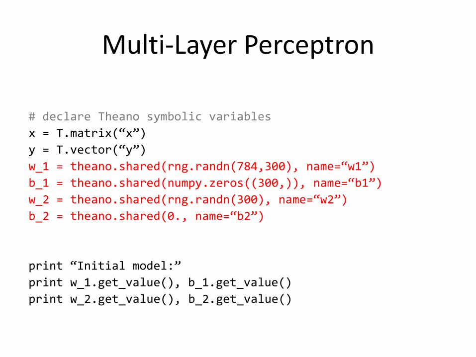
Multi-Layer Perceptron

# declare Theano symbolic variables

x = T.matrix(“x”)

y = T.vector(“y”)

w_1 = theano.shared(rng.randn(784,300), name=“w1”)

b_1 = theano.shared(numpy.zeros((300,)), name=“b1”)

w_2 = theano.shared(rng.randn(300), name=“w2”)

b_2 = theano.shared(0., name=“b2”)

print “Initial model:”

print w_1.get_value(), b_1.get_value()

print w_2.get_value(), b_2.get_value()

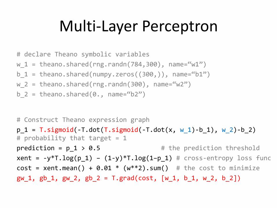
Multi-Layer Perceptron

# declare Theano symbolic variables

w_1 = theano.shared(rng.randn(784,300), name=“w1”)

b_1 = theano.shared(numpy.zeros((300,)), name=“b1”)

w_2 = theano.shared(rng.randn(300), name=“w2”)

b_2 = theano.shared(0., name=“b2”)

# Construct Theano expression graph

p_1 = T.sigmoid(-T.dot(T.sigmoid(-T.dot(x, w_1)-b_1), w_2)-b_2) # probability that target = 1

prediction = p_1 > 0.5 # the prediction threshold

xent = -y*T.log(p_1) – (1-y)*T.log(1–p_1) # cross-entropy loss func

cost = xent.mean() + 0.01 * (w**2).sum() # the cost to minimize

gw_1, gb_1, gw_2, gb_2 = T.grad(cost, [w_1, b_1, w_2, b_2])

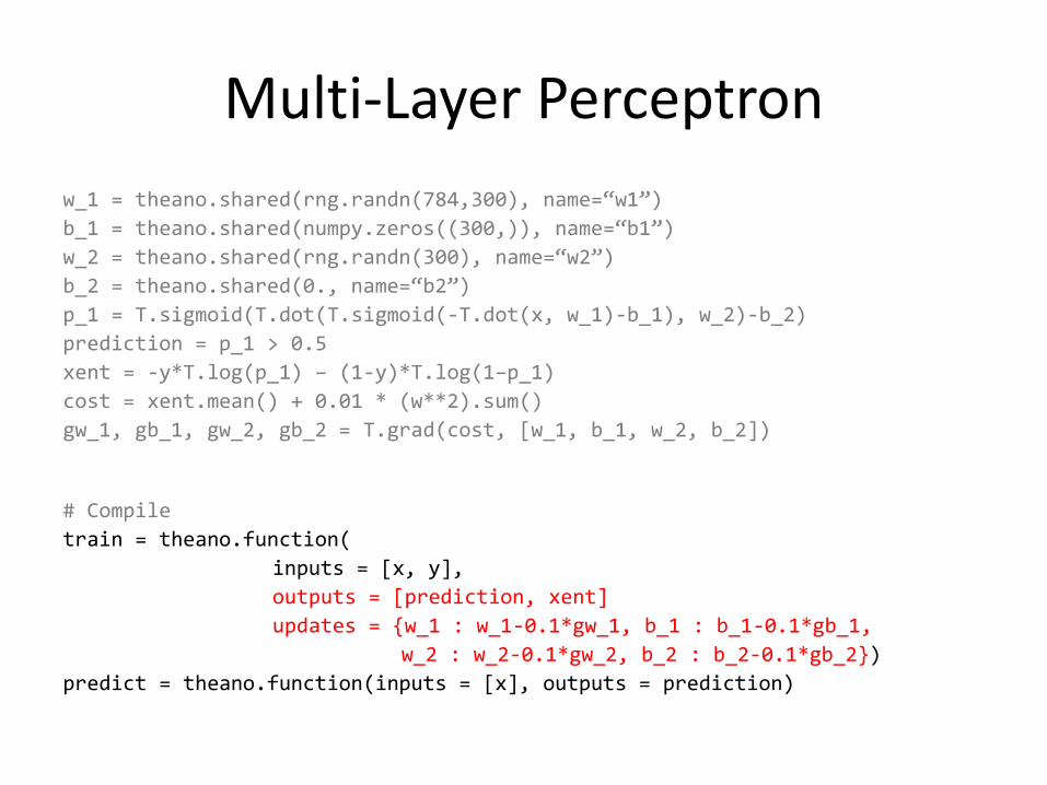
Multi-Layer Perceptron

w_1 = theano.shared(rng.randn(784,300), name=“w1”)

b_1 = theano.shared(numpy.zeros((300,)), name=“b1”)

w_2 = theano.shared(rng.randn(300), name=“w2”)

b_2 = theano.shared(0., name=“b2”)

p_1 = T.sigmoid(T.dot(T.sigmoid(-T.dot(x, w_1)-b_1), w_2)-b_2)

prediction = p_1 > 0.5

xent = -y*T.log(p_1) – (1-y)*T.log(1–p_1)

cost = xent.mean() + 0.01 * (w**2).sum()

gw_1, gb_1, gw_2, gb_2 = T.grad(cost, [w_1, b_1, w_2, b_2])

# Compile

train = theano.function(

inputs = [x, y],

outputs = [prediction, xent]

updates = {w_1 : w_1-0.1*gw_1, b_1 : b_1-0.1*gb_1,

w_2 : w_2-0.1*gw_2, b_2 : b_2-0.1*gb_2})

predict = theano.function(inputs = [x], outputs = prediction)

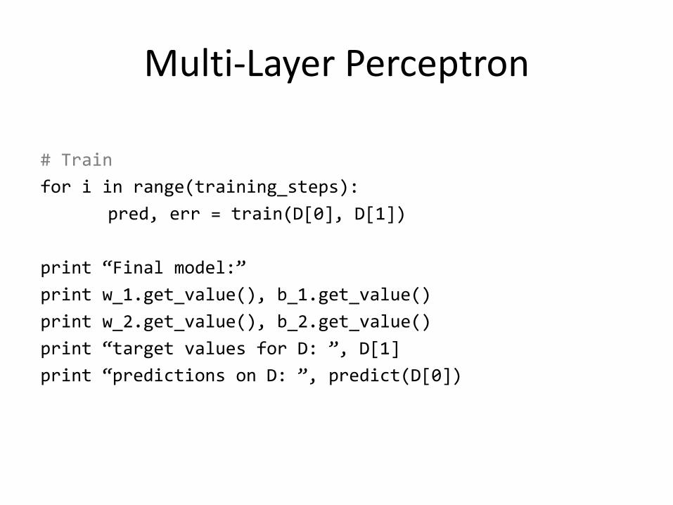
Multi-Layer Perceptron

# Train

for i in range(training_steps):

pred, err = train(D[0], D[1])

print “Final model:”

print w_1.get_value(), b_1.get_value()

print w_2.get_value(), b_2.get_value()

print “target values for D: ”, D[1]

print “predictions on D: ”, predict(D[0])

CASE STUDY - 3 Recurrent Neural Network

Recurrent Neural Network

• Exercise

– Use scan to implement the loop operation

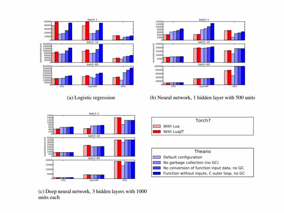
COMPARISON WITH OTHER TOOLKITS

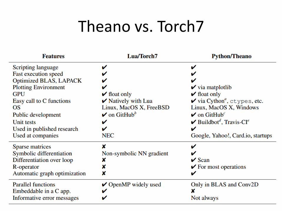
Theano vs. Torch7

Thank you!