Available online at www.sciencedirect.com

www.elsevier.com/locate/asr

ScienceDirect

Advances in Space Research 55 (2015) 125–134

A simplified and unified model of multi-GNSS precise point positioning

Junping Chen a,⇑, Yize Zhang a,b, Jungang Wang a,b, Sainan Yang a, Danan Dong c,Jiexian Wang b, Weijing Qu a, Bin Wu a

a Shanghai Astronomical Observatory, Chinese Academy of Sciences, Shanghai 200030, PR Chinab College of Surveying and Geo-informatics Engineering, Tongji University, Shanghai 200092, PR China

c School of Information Science & Technology, East China Normal University, Shanghai 200242, PR China

Received 6 July 2014; received in revised form 19 September 2014; accepted 7 October 2014Available online 20 October 2014

Abstract

Additional observations from other GNSS s can augment GPS precise point positioning (PPP) for improved positioning accuracy,reliability and availability. Traditional multi-GNSS PPP model requires the estimation of inter-system bias (ISB) parameter. Basedon the scaled sensitivity matrix (SSM) method, a quantitative approach for assessing parameter assimilation, we theoretically prove thatthe ISB parameter is not correlated with coordinate parameters and it can be assimilated into clock and ambiguity parameters. Thus,removing ISB from multi-GNSS PPP model does not affect coordinate estimation. Based on this analysis, we develop a simplifiedand unified model for multi-GNSS PPP, where ISB parameter does not need to be estimated and observations from different GNSS sys-tems are treated in a unified way. To verify the new model, we implement the algorithm to the self-developed software to process 1 yearGPS/GLONASS data of 53 IGS (International GNSS Service) worldwide stations and 1 month GPS/BDS data of 15 IGS MGEX(Multi-GNSS Experiment) stations. Two types of GPS/GLONASS and GPS/BDS combined PPP solution are performed, one is basedon traditional model and the other implements the new model. RMSs of coordinate differences between the two type of solutions are fewlm for daily static PPP and less than 0.02 mm for GPS/GLONASS kinematic PPP in the North, East and Up components, respectively.Considering the millimeter-level precision of current GNSS PPP solutions, these statistics demonstrate equivalent performance of the twosolution types.� 2014 COSPAR. Published by Elsevier Ltd. All rights reserved.

Keywords: Multi-GNSS; MGEX; Precise point position; Inter-system bias; Scaled sensitivity matrix

1. Introduction

Precise point positioning (PPP) using global positioningsystem (GPS) measurements achieves accuracy for staticand kinematic stations at the millimeter to decimeter levels,respectively (Zumberge et al., 1997; Bisnath and Gao,2009). With the development of navigation systems andtracking infrastructure, PPP using multi-system observa-tions has become increasingly popular (Dach et al., 2009,2010; Pıriz et al., 2009; Melgard et al., 2009; Cai andGao, 2013; Chen et al., 2013). Multi-GNSS (Global

http://dx.doi.org/10.1016/j.asr.2014.10.002

0273-1177/� 2014 COSPAR. Published by Elsevier Ltd. All rights reserved.

⇑ Corresponding author.

Navigation Satellite Systems) PPP could improve solutionavailability by improving tracking geometry, especially inenvironment like urban canyon and ravines. On the otherhand, it improves positioning accuracy as it has moreobservations and it largely eliminate existing positionerrors introduced by the periodic regression of satellite con-stellations (Flohrer, 2008).

Many manufacturers are providing multi-GNSS receiv-ers, however, most geodetic receivers and antennas are notcalibrated, which leaves instrument hardware delayunknown. In the GPS-only data processing, the instrumenthardware delay is assimilated into receiver clock and doesnot affect position estimates. In multi-GNSS data process-

126 J. Chen et al. / Advances in Space Research 55 (2015) 125–134

ing, however, the hardware delay is different for satellitesystems even for the same type of receiver/antenna pair(Wanninger, 2012; Chen et al., 2013). Therefore, multi-GNSS data analysis requires the estimates of clock param-eter together with additional inter-system bias (ISB)parameter. However, there are no conventional modelsfor the estimation of ISB parameters within the IGS com-munity. As a matter of result, the GLONASS satelliteclocks of IGS Analysis Centers (ACs) differ in temporalreference frame or clock consistency (Schaer, 2014). TheISB results in the station clock differences when processingeach system separately, and it includes the impacts of thesystem-dependant hardware delay terms of both stationand satellite.

Therefore there should be as many clock parameters asmany satellite systems that a station observes. Recentinvestigation shows that the difference of hardware delaybetween satellite systems is stable over daily interval forthe same station (Dach et al., 2009, 2010; Wanninger,2012). The clock parameter is normally treat as epoch-wiseparameter, while ISB parameter is treated as daily constant(Cai and Gao, 2013; Chen et al., 2013). In case of GLON-ASS observations involved, there are additional inter-fre-quency bias (IFB) parameters caused by the frequencydifferences between satellites (Wanninger, 2012; Shi et al.,2013). Taking the IFBs into account, theoretically thereshould be as many ISB parameters as many GLONASSfrequencies that a station tracks in GPS/GLONASS com-bined PPP. In practice, one ISB parameter is sufficient asthe IFB parameter is assimilated into ambiguity parame-ters (Dach et al., 2010; Cai and Gao, 2013). This strategyis currently most used for the multi-GNSS PPP and hasproved to be very promising (Melgard et al., 2009; Pırizet al., 2009; Dach et al., 2010; Cai and Gao, 2013).

In this paper, we analyze the correlation coefficientsbetween ISB parameter and other parameters and applythe quantitative scaled sensitivity matrix (SSM) approach(Dong et al., 2002) for assessing the influences of unre-solved ISB parameter on other parameters. Results showthat there is no correlation between ISB parameter andcoordinate parameters, and the ISB values can be fullyassimilated into clock and ambiguity parameters. Basedon this analysis, we develop a new multi-GNSS PPP modelwhich does not include ISB parameter and observations ofdifferent GNSS systems are treated in a unified way. Toverify and test the new model, we implement it to theLTW_BS software (Wang and Chen, 2011) to process1 year GPS/GLONASS data of 53 IGS (InternationalGNSS Service, Dow et al., 2009) stations and 1 monthGPS/BDS data of 15 IGS MGEX (Multi-GNSS Experi-ment) stations. Two types of GPS/GLONASS and GPS/BDS combined PPP solutions are performed, one uses tra-ditional model and the other implements the new model.Results from the two models show equivalent results,which demonstrates the efficiency and correctness of thenew model. In the following, Section 2 presents the tradi-tional multi-GNSS PPP model; Section 3 presents the

new multi-GNSS PPP model; Section 4 presents data anal-ysis and compares daily positioning qualities; finally, Sec-tion 5 summarizes the main points of this paper anddiscuss the perspectives of the new model.

2. Multi-GNSS PPP model based on ISB estimation

Multi-GNSS PPP refers to the combined PPP usingobservations from more than one satellite system, whereprecise satellite orbits and clocks are available. In the fol-lowing formulas we use GPS/GLONASS PPP as an exam-ple, and the conclusions apply to the combined PPP forother systems as well.

2.1. GPS PPP model

The ionosphere-free (IF) pseudo-range and phase obser-vation functions between a receiver and a GPS satellite Gcan be written as:

P G¼ qGþ c � ðdtG�dtGÞþðbG�bGÞþmG �ZTDGþ 1G

LG¼ qGþ c � ðdtG�dtGÞþðBG�BGÞþN GþmG �ZTDGþ eG

ð1Þ

where P G; LG are respectively pseudo-range and carrierphase IF observation; qG is geometrical distance, c is lightspeed; dtG is receiver clock offset, dtG is satellite clock offset;bG; bG and BG; BG are the IF combined pseudo-range andcarrier phase hardware delay bias for satellites (�G) andreceivers (�G); N G is ambiguity in meters, mG and ZTDG

are mapping function and zenith tropospheric delay, 1G

and eG are noise.The pseudo-range observation in (1) provides the refer-

ence to clock parameters. For GPS observations, thepseudo-range hardware delay biases bG; bG are assimilatedinto the clock offset c � ðdtG � dtGÞ following the IGS anal-ysis convention. The carrier phase hardware delay biasesBG; BG are not considered in most GPS data processing.The carrier phase hardware bias is satellite dependentand stable over time, thus it is grouped into ambiguity(Defraigne and Bruyninx, 2007; Dach et al., 2010; Genget al., 2010a). After applying the GPS precise satelliteorbits and clocks, (1) can be rewritten as:

P G ¼ qG þ c � d�tG þ mG � ZTDG þ 1G

LG ¼ qG þ c � d�tG þ �N G þ mG � ZTDG þ eGð2Þ

where d�tG and �NG are reformed station clock and ambigu-ity with:

c � d�tG ¼ c � dtG þ bG

�NG ¼ NG þ BG � bG

ð3Þ

In (2), the satellite hardware delays are contained in theprecise satellite clocks and are removed at the user sitewhen applying the precise products (Defraigne andBruyninx, 2007). Eq. (2) illustrates GPS PPP observationequation, where we see that ambiguity term is not an

J. Chen et al. / Advances in Space Research 55 (2015) 125–134 127

integer as it contains the bias term, and the term BG � bG

refers to the un-calibrated phase delay (Ge et al., 2008).Eqs (2) and (3) apply to other GNSS systems like BDSand Galileo providing CDMA (Code Division MultipleAccess) signals.

2.2. GLONASS PPP model

Extending (1) to GLONASS observations and applyingthe GLONASS precise satellite orbits and clocks, IF obser-vation functions between a receiver and a GLONASS satel-lite R can be written as:

P R ¼ qR þ c � dtR þ bR þ mR � ZTDR þ 1R

LR ¼ qR þ c � dtR þ BR þ N R þ mR � ZTDR þ eRð4Þ

Compared with (1), superscript changes from G (repre-senting GPS) to R (representing GLONASS). The meaningof each term is similar, but now all refer to GLONASSobservations.

Unlike GPS, GLONASS provides frequency divisionmultiple access (FDMA) signal, which results in frequencydifferences between GLONASS satellites. Consequently,instrument hardware delays are different for a stationtracking GLONASS satellites with different frequencychannels (Wanninger, 2012; Chen et al., 2013; Shi et al.,2013). Hardware delay can be rewritten as a sum of a meanterm and a frequency-dependent bias term as given below(Cai and Gao, 2013):

bR ¼ bavgR þ dbR; BR ¼ Bavg

R þ dBR ð5ÞIn (5), bavg

R and BavgR are the mean hardware delay for

pseudo-range and phase observations. The satellite-depen-dent bias terms dbR; dBR are referred to inter-frequencybias. Substituting (5) into (4), we have the GLONASSobservation equation:

P R ¼ qR þ c � d�tR þ dbR þ mR � ZTDR þ 1R

LR ¼ qR þ c � d�tR þ �NR þ mR � ZTDR þ eRð6Þ

where d�tR and �N R are reformed station clock offset andambiguity with:

c � d�tR ¼ c � dtR þ bavgR

�N R ¼ N R þ BavgR � bavg

R þ dBRð7Þ

Similar to the GPS equation of (3), the mean pseudo-range hardware delay is assimilated into clock parameterand the difference between mean pseudo-range and phasehardware delay is assimilated into ambiguity parameter.The phase IFB term is treated as fractional parts of hard-ware delay and is assimilated into ambiguity term (Genget al., 2010a; Dach et al., 2010; Cai and Gao, 2013). Eq.(6) contains the pseudo-range IFB term dbR, which is satel-lite dependent and could not be grouped with other param-eters. Theoretically, the GLONASS pseudo-range IFBcould be set up as frequency-dependent unknowns in PPPprocessing. But this will introduce too many unknownparameters and the precision depends on the precision of

pseudo-range observations. Because pseudo-range observa-tions is normally assigned a much smaller weight comparedto the carrier phase observations in GNSS data processing,dbR can therefore be neglected and its effect will show up inthe pseudo-range residuals (Geng et al., 2010a; Cai andGao, 2013). The final GLONASS PPP observation equa-tion can be rewritten as:

P R ¼ qR þ c � d�tR þ mR � ZTDR þ 1R

LR ¼ qR þ c � d�tR þ �NR þ mR � ZTDR þ eRð8Þ

2.3. Traditional GPS/GLONASS PPP model

The traditional GPS/GLONASS PPP model requiresthe estimation of an additional inter-system bias parame-ter, the ionosphere-free (IF) pseudo-range and phase obser-vations for the combined GPS/GLONASS PPP can bewritten as:

P G ¼ qG þ c � d�tG þ mG � ZTDþ 1G

LG ¼ qG þ c � d�tG þ �N G þ mG � ZTDþ eG

P R ¼ qR þ c � d�tG þ ISBþ mR � ZTDþ 1R

LR ¼ qR þ c � d�tG þ ISBþ �N R þ mR � ZTDþ eR

ð9Þ

In (9), the inter-system bias parameter is defined asfollowing,

ISB ¼ c � d�tR � c � d�tG ¼ c � dtR � c � dtG þ bavgR � bG ð10Þ

This model has been applied in GPS/GLONASS com-bined PPP and is proved be more accurate and more robustthan single system solution.

The modeling of ISB parameter could be in differentway: as daily constant, piece wise constant (PWC) orepoch wise variable. For rigorous data analysis, epoch-wise ISB should be estimated. But this will introducetoo many unknowns and reduce the efficiency of the solu-tion. Dach et al. (2010) conducted detailed analysis onthe modeling of ISB parameter by making double differ-ence for stations equipped with different receivers. Theyshow that the coordinate differences applying differentISB models are less than 2 mm in worst case. Consideringthe current PPP accuracy limits, we could conclude fromtheir results that daily constant ISB model is sufficient formulti-GNSS PPP.

3. Simplified and unified multi-GNSS PPP model

The solution of (9) could be performed based on theleast-square estimation with the complete normal equationcontaining all parameters generated. Based on the normalequation, we analyze the correlation coefficients betweenparameters. We use data of the station LPGS (La Plata,Argentina) on DOY 309, 2012. Estimated parametersinclude: epoch-wise station clock and static coordinates,ZTD parameter in PWC at interval of 1 h, and ISB param-eter as daily constant.

Table 1Correlation coefficients between ISB and other parameters of GPS/GLONASS PPP.

X Y Z ZTD d�tIF ;G �NGIF

�NRIF

ISB �1E�5 2E�5 1E�5 2E�5 �0.65 0.65 �0.76

128 J. Chen et al. / Advances in Space Research 55 (2015) 125–134

We use the following function to calculate correlationcoefficient between parameters:

r ¼ rABffiffiffiffiffiffiffiffiffiffirArBp ð11Þ

where rA, rB, rAB are the variance and co-variance elementsof parameters A and B based on the normal equation.

Fig. 1 shows the correlation coefficients between ISBparameter and coordinate parameters at first 100 epochs,where the coefficients converge to zero after the first 4epochs.

Table 1 summarize the correlation coefficients betweenISB and the other parameters of the last epoch of the dailyprocessing. As shown in Table 1, the ISB/coordinate andISB/ZTD correlation coefficients are near zero, which sug-gests that there is no correlation between ISB and theseparameters. Therefore, we could remove ISB term in (9).However, the removal of ISB term introduces the changeof other parameters, i.e., parameters like ambiguities andclocks will change in order to account for this new param-eterization model.

To further prove the above statement and to have aquantitative gauge of the parameter assimilation, we usethe SSM (Scaled Sensitivity Matrix) method (Dong et al.,2002), which is a quantitative approach for assessing theinfluences of unresolved parameters. Following Donget al. (2002), we write (9) in the following form,

y ¼ A1 � X 1 þ A2 � X 2 ð12Þ

where X 2 is defined as the ISB parameter and could beremoved from (12), X 1 includes the other parameters;A1; A2 are design matrices for corresponding parameters.The corresponding normal equation is,

N 11 N 12

N 21 N 22

� ��

X 1

X 2

� �¼

u1

u2

� �ð13Þ

Fig. 1. Correlation coefficients between ISB parameter and coordinateparameters.

According to Dong et al. (2002), since X 2 could not beresolved from the observations y, we actually solve thefollowing normal equation

N 11X 1 ¼ u1 ð14Þ

the rigorous least squares solution of X 1 yields

X 1 ¼ N�111 � u1 ð15Þ

Replacing u1 in (15) by (13), we obtain

X 1 ¼ X 1 þ N�111 � N 12 � X 2 ð16Þ

Eq. (16) indicates that the estimated values of X 1 areactually the linear combinations of X 1 and X 2 in (13).And N�1

11 � N 12 are the elements of the scaled sensitivitymatrix, which quantitatively defines the ratio of X 2 thatassimilates to each parameter of X 1.

We calculate the scaled sensitivity matrix using the nor-mal equation of LPGS in the above analysis and results areshown in Table 2, where the element of ISB/ �N G

IF is the samefor all GPS satellites and element of ISB/ �NR

IF is the same forall GLONASS satellites.

According to Table 2, less than 10�6 parts of ISB willassimilate into coordinate parameters, which accounts toless than 1 mm for most present receivers. Less than 10�8

parts of ISB will assimilate into ZTD parameter, thusZTD will not be affected by the removal of ISB.

Around 42.2% of ISB is absorbed by the clock parame-ter and accordingly the same amount is absorbed by GPSambiguity parameter but with opposite sign. Thus theinfluence of the ISB removal for the GPS equations in (9)reflects on clock and ambiguity parameters and their influ-ence compensates for each other.

Another 57.8% of ISB is absorbed by GLONASS ambi-guity parameter. Sum the scaled sensitivity matrix elementof ISB/clock and ISB/GLONASS ambiguity, we have57:8%þ 42:2% ¼ 100%. This confirms that the sum ofscaled element, which represents ratio of ISB parameterassimilated into station clock and GLONASS ambiguityparameters, equals to the original ISB in (9). Thus theinfluence of the ISB removal for the GLONASS equationsin (9) reflects also on the clock and ambiguity parametersand the sum of their changes equal to the original ISBterms.

Based on the above discussion, the ISB in (9) could beremoved and (9) could be re-written as:

P G ¼ qG þ c � d�tC þ mG � ZTDþ 1G

LG ¼ qG þ c � d�tC þ �NGC þ mG � ZTDþ eG

P R ¼ qR þ c � d�tC þ mR � ZTDþ 1R

LR ¼ qR þ c � d�tC þ �N RC þ mR � ZTDþ eR

ð17Þ

Table 2Elements of the scaled sensitivity matrix between ISB and other parameters.

X Y Z ZTD d�tIF ;G �NGIF

�NRIF

ISB �1E�7 6E�7 8E�7 8E�9 0.422 �0.422 0.578

J. Chen et al. / Advances in Space Research 55 (2015) 125–134 129

where, d�tC is defined as new clock, �N Gl and �N R

l are newambiguity terms and the other terms remain unchanged.

Eq. (17) is the simplified observation function of GPS/GLONASS PPP processing, it applies to the multi-GNSSPPP of other satellite systems. In the new model, observa-tions of different GNSS systems is processed in an unifiedway as they were of the same system, and the ISB is assim-ilated into the clock and ambiguity parameter. Due to themuch smaller weight assigned on pseudo-range observa-tions compared to phase observations, all pseudo-rangeobservations show big residuals and this may slow downthe convergence of PPP (Geng et al., 2010b, 2011). TheGPS pseudo-range residuals are close to the amount ofISB value that assimilated into the station clock parameter.The GLONASS pseudo-range residuals are close to theamount of ISB value that assimilated into the GLONASSambiguity.

4. Data processing

To validate the new PPP model, we perform GPS/GLONASS daily static PPP for 53 IGS reference stationsusing data of the whole year of 2012. GPS/GLONASSkinematic PPP is performed using 1 month (January2012) data of the 53 stations. In addition we performGPS/BDS daily static PPP using 1 month (March, 2013)data of 15 IGS MGEX stations. Fig. 2 shows the distribu-tion of the 68 stations.

For results evaluation and comparison, data process-ing is performed in the following four scenarios: GPS-only PPP, GLONASS-only PPP, traditional GPS/GLONASS and GPS/BDS combined PPP with ISBestimated as daily constant, and GPS/GLONASS andGPS/BDS combined PPP using the new model withno ISB estimated.

Fig. 2. The distribution of the used stations, read stars (G+R) illustrate GP

Moreover, precise satellite orbits and clocks from ESA,GFZ and SHA (Chen et al., 2012, 2014) are used for GPS/GLONASS PPP. Precise satellite orbits and clocks fromGFZ and SHA are used for GPS/BDS PPP. We use thesesatellite products, rather than IGS ones, is to avoid the pos-sible inhomogeneities of the IGS final products which candegrade the positioning quality of PPP (Teferle et al.,2007). For data modeling, we applied the absolute phasecenters (Schmid et al., 2007), the phase-wind up effects(Wu et al., 1993) and the station displacement models pro-posed by the IERS conventions 2010 (Petit and Luzum,2010). A cut-off angle of 7� was set for usable measure-ments and data sampling is set to 60 s. An elevation-depen-dent weighting strategy was applied to measurements atlow elevations. Moreover, we estimated ZTD parameterevery 1 h by applying the most recently developed GPT2empirical slant delay model (Lagler et al., 2013). Animproved version of the LTW_BS software was used(Wang and Chen, 2011).

In this following, we present how the traditional andnew models agree in PPP positioning results. All the fol-lowing results are based on the precise products of SHA,and PPP results based on GFZ and ESA products supportthe same conclusion.

4.1. Position differences between daily static PPP and IGS

daily solutions

We compared our GPS/GLONASS daily position esti-mates with the IGS daily solutions through a 7-parameterHelmert transformation (Teferle et al., 2007; Geng et al.,2010a). We removed those position estimates with trans-formed residuals larger than five times the standard devia-tions, which amounts to less than 0.7% (118 out of 18,551

S/GLONASS stations and green points (G+C) are GPS/BDS stations.

Fig. 3. Number and value of outliers in Helmert transformation between daily PPP and IGS daily solution over 1 year. PPP solutions are performed inGPS-only, GLONASS-only and GPS/GLONASS combined mode.

Table 3Mean RMS statistics (in mm) of residuals of the daily PPP positionestimates against the IGS daily solutions in 2012.

GPS-only GLONASS-only G/G trad. G/G new

North 5.3 7.4 5.3 5.3East 8.2 8.8 7.0 7.0Up 15.2 18.3 13.4 13.4

130 J. Chen et al. / Advances in Space Research 55 (2015) 125–134

points). Fig. 3 shows the outliers in Helmert transformation,where the number of outliers are 168, 218 and 118 for GPS,GLONASS and GPS/GLONASS PPP, respectively. Also,the GPS/GLONASS combined PPP using new and tradi-tional model is nearly the same and their values differ atthe level of lm.

RMS statistics of the transformed residuals are used toquantitatively assess the extrinsic positioning quality. Theupper plot of Fig. 4 shows for all stations the RMS statis-tics of coordinate differences between GPS/GLONASSPPP and IGS daily solutions. Table 3 shows the meanRMS statistics of all days for the four scenarios, wherewe see GPS/GLONASS combined PPP improves theRMS statistics by up to 28% compared to the single system

Fig. 4. (a) RMS statistics of coordinate differences between GPS/GLONASSDifferences of the RMS statistics of traditional and new model for each stationthe IGS daily solutions over 1 year.

PPP. The RMS statistics of GPS/GLONASS combinedPPP using the new and traditional model are almost thesame, and the bottom plot of Fig. 4 shows their RMS dif-ferences for each station. In this plot, the RMS differencesare less than 1 lm in each coordinate component, verifying

daily static PPP and IGS daily solution for each station over one year. (b). A RMS is computed over the residuals of PPP position estimates against

J. Chen et al. / Advances in Space Research 55 (2015) 125–134 131

the same PPP position estimates are derived from these twomodels.

4.2. Position differences of daily static PPP between

traditional and new model

Assessing the differences between the position estimatescan directly illustrate to what extent these two models agreein their positioning results. In the following we comparethe GPS/GLONASS and GPS/BDS daily static PPPresults of the traditional and new models.

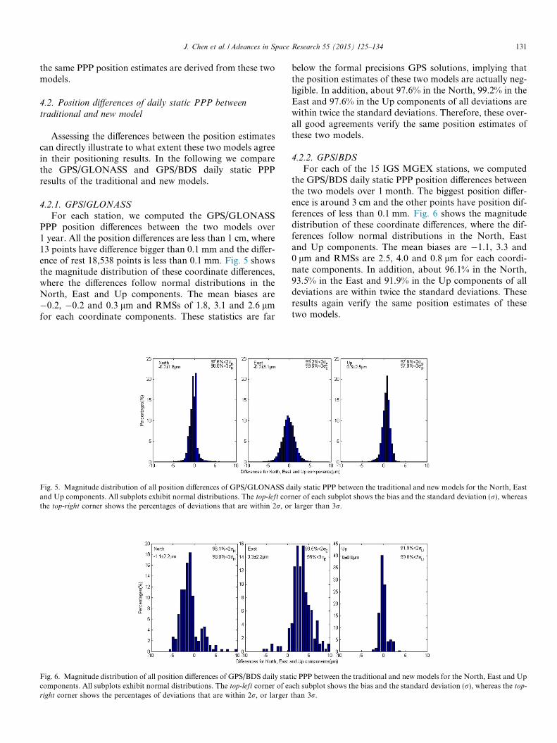
4.2.1. GPS/GLONASS

For each station, we computed the GPS/GLONASSPPP position differences between the two models over1 year. All the position differences are less than 1 cm, where13 points have difference bigger than 0.1 mm and the differ-ence of rest 18,538 points is less than 0.1 mm. Fig. 5 showsthe magnitude distribution of these coordinate differences,where the differences follow normal distributions in theNorth, East and Up components. The mean biases are�0.2, �0.2 and 0.3 lm and RMSs of 1.8, 3.1 and 2.6 lmfor each coordinate components. These statistics are far

Fig. 5. Magnitude distribution of all position differences of GPS/GLONASS dand Up components. All subplots exhibit normal distributions. The top-left corthe top-right corner shows the percentages of deviations that are within 2r, or

Fig. 6. Magnitude distribution of all position differences of GPS/BDS daily statcomponents. All subplots exhibit normal distributions. The top-left corner of earight corner shows the percentages of deviations that are within 2r, or larger

below the formal precisions GPS solutions, implying thatthe position estimates of these two models are actually neg-ligible. In addition, about 97.6% in the North, 99.2% in theEast and 97.6% in the Up components of all deviations arewithin twice the standard deviations. Therefore, these over-all good agreements verify the same position estimates ofthese two models.

4.2.2. GPS/BDS

For each of the 15 IGS MGEX stations, we computedthe GPS/BDS daily static PPP position differences betweenthe two models over 1 month. The biggest position differ-ence is around 3 cm and the other points have position dif-ferences of less than 0.1 mm. Fig. 6 shows the magnitudedistribution of these coordinate differences, where the dif-ferences follow normal distributions in the North, Eastand Up components. The mean biases are �1.1, 3.3 and0 lm and RMSs are 2.5, 4.0 and 0.8 lm for each coordi-nate components. In addition, about 96.1% in the North,93.5% in the East and 91.9% in the Up components of alldeviations are within twice the standard deviations. Theseresults again verify the same position estimates of thesetwo models.

aily static PPP between the traditional and new models for the North, Eastner of each subplot shows the bias and the standard deviation (r), whereaslarger than 3r.

ic PPP between the traditional and new models for the North, East and Upch subplot shows the bias and the standard deviation (r), whereas the top-

than 3r.

Fig. 7. Coordinate differences of kinematic PPP between the traditional and new models for ADIS, DOY 3, 2012. (a) The first 100 epochs. (b) From the100th epoch to the end of day.

Fig. 8. Magnitude distribution of all coordinate differences of GPS/GLONASS kinematic PPP between the traditional and new models for the North,East and Up components. All subplots exhibit normal distributions. The top-left corner of each subplot shows the bias and the standard deviation (r),whereas the top-right corner shows the percentages of deviations that are within 2r, or larger than 3r.

132 J. Chen et al. / Advances in Space Research 55 (2015) 125–134

4.3. Position differences of kinematic PPP betweentraditional and new model

GPS/GLONASS kinematic PPP is performed using onemonth data of the 53 stations. Kinematic PPP resultsbetween the new and traditional models are analyzed. Wefirst analyze the convergence of the two models. It is foundthat the convergences are quite close to each other. Onaverage the position difference is less than 0.1 m after 2.4epochs and less than 1 mm after 18.1 epochs. Fig. 7 showsthe kinematic position difference of station ADIS (AddisAbaba, Ethiopia) on DOY 3, 2012. From the left plot ofFig. 7, we see that coordinate differences are less than0.1 m after 3 epochs, while the right plot shows that thecoordinate differences after the 100th epoch.

To assess the differences of the kinematic position esti-mates, we analyze the epoch-wise coordinates after the first100 epochs, which are regarded as convergence period ofkinematic PPP. All the position differences are less than1 cm, where 1870 out of 1,814,500 (�0.1%) points have dif-ference bigger than 1 mm and the difference of rest points isless than 1 mm. Fig. 8 shows the magnitude distribution ofthe epoch-wise coordinate differences for all stations over1 month, where the differences follow normal distributionsin the North, East and Up components. The mean biasesare 0.6, 1.1 and �1.1 lm and RMSs are 13.8, 15.2 and

13.1 lm for each coordinate components. Moreover, about96.2% in the North, 96.4% in the East and 96.6% in the Upcomponents of all deviations in Fig. 8 are within twice thestandard deviations. Thus, all these overall good agree-ments verify the same kinematic position estimates of thesetwo models.

4.4. Differences of other parameters between traditional and

new model

In the new multi-GNSS PPP model, the station clockand ambiguity estimates are different from that of the tra-ditional model. These two parameters actually absorb theISB parameters, and the percentage which goes into eachparameter depends on the normal equation. Therefore, itis difficult to compare these parameters directly and havemeaningful conclusion. The parameter assimilation hasopposite sign for the GPS observations, thus the sum ofstation clock and GPS ambiguity should theoretically bethe same for the traditional and new model. Therefore,we compare the sum of station clock and GPS ambiguityfrom the two models. The upper subplot of Fig. 9 showsthe magnitude distribution of the differences for all GPSsatellite/station pairs at the last epoch on all days. Themean difference is 0.1 lm and all the differences are below3 cm with 99 out of 177,644 differences bigger than 1 mm.

Fig. 9. Magnitude distribution of differences between the traditional and new models of (a) sum of GPS ambiguity and station clock parameters; (b) sumof GLONASS ambiguity, ISB and station clock parameters. Both plots exhibit normal distributions. The top-left corner of each subplot shows the biasand the standard deviation (r), whereas the top-right corner shows the percentages of deviations that are within 2r, or larger than 3r.

J. Chen et al. / Advances in Space Research 55 (2015) 125–134 133

For GLONASS and BDS observations, the sum ofstation clock and ambiguity from the new model shouldtheoretically be the same as the sum of station clock,ISB and ambiguity of the traditional model. The bottomsubplot of Fig. 9 shows the magnitude distribution ofthe differences for all GLONASS satellite/station pairsat the last epoch on all days. The mean difference is lessthan 0.1 lm and all the differences are below 1 mm with73 out of 143,759 differences are bigger than 1 mm. Bothplots show that the differences are so small, which fur-ther proves correctness of the parameter assimilationanalysis and ensure the same coordinate estimates inthese two models.

5. Conclusions and suggestions

In this study, we analysis the parameter correlations inmulti-GNSS PPP and prove that the ISB parameter isnot correlated with the coordinate and ZTD parameters.We rigorously analyze the parameter assimilation propertywhen the ISB parameter is removed from the multi-GNSSPPP. Results show that the ISB parameter is totally assim-ilated into station clock and ambiguity parameters andnone of ISB is absorbed by coordinate estimates. Basedon these analysis, a new simplified and unified model isdeveloped for multi-GNSS PPP.

In this new model, the ISB parameter is not explicitlydefined rather it is removed in the GNSS observation equa-tion. Applying the new model, observations of differentGNSS system are treated in a unified way as they were ofthe same satellite system. In order to verify this new modeland prove the equivalence of coordinate estimates, we com-pute GPS/GLONASS and GPS/BDS PPP position esti-mates using the traditional and new models with 1 yearGPS/GLONASS data of 53 IGS stations and 1 monthGPS/BDS data of 15 IGS MGEX stations.

Comparing daily static coordinate estimates betweentraditional and new models, mean biases of the differencesare �0.2, �0.2 and 0.3 lm for GPS/GLONASS PPP, �1.1,3.3 and 0 lm for GPS/BDS PPP, whereas the RMSs are1.8, 3.1 and 2.6 lm for GPS/GLONASS PPP, 2.5, 4.0and 0.8 lm for GPS/BDS PPP in the North, East andUp components respectively. Comparisons of GPS/GLONASS kinematic coordinate estimates between thetwo models shows mean bias of 0.6, 1.1 and -1.1 lm andRMSs of 13.8, 15.2 and 13.1 lm in the North, East andUp components respectively. The results show the coordi-nate differences between the two models are actually negli-gible, and the closeness of the coordinate estimates andRMS statistics against the IGS daily solutions overall ver-ify the equivalence of the position estimates derived fromthe traditional and new models.

We have used the precise GNSS products of the GNSSanalysis centers of ESA, GFZ and SHA for all the abovetests. The orbit differences among these centers is at levelof few cm, while their differences in satellite clocks aremuch bigger. This is because different strategies are appliedin their ISB parameters handling and the temporal refer-ence frames are also different. Nevertheless, the conclusionis the same. We have used GPS/GLONASS and GPS/BDSdata to verify the new model, but it applies to the combinedPPP for other GNSS systems.

Beside the equivalence results of the two models, thereare potential advantages of the new model:

(1) Under some extreme circumstances, the traditionalmulti-GNSS PPP model may fail due to rank defi-ciency. For example, in the situation where only 4 sat-ellites (at least one GPS and one GLONASS satellite)could be observed. Our multi-GNSS PPP approachmight still obtain solutions due to omitting the ISBterm (remedy the rank deficiency).

134 J. Chen et al. / Advances in Space Research 55 (2015) 125–134

(2) The correlation between the clock and ambiguityparameters are reduced, thus stabilizing the solutionusing the new model.

(3) Multi-GNSS PPP realization is simplified and uni-fied. Under this new model, observations of differentGNSS system are treated in a unified way as theywere of the same satellite system. Multi-GNSS PPPcould be conveniently implemented in current singlesystem PPP software module.

Implementing the new model the ambiguity and stationclock absorb parts of the ISB, consequently the traditionalPPP ambiguity fixing approach using un-differenced obser-vations may not work. However, we could use theapproach by making single-difference between two satel-lites of the same system for PPP ambiguity fixing followingour new model. By making satellite-difference, the amountof ISBs assimilated into ambiguities are canceled out andthe strategy of between-satellite integer ambiguity fixingcould be developed.

Acknowledgments

Editor in chief Pascal Willis and three anonymousreviewers are acknowledged for their valuable suggestions.IGS community is acknowledged for providing RINEXdata and orbit and clock products. This research is sup-ported by 100 Talents Programme of the Chinese Academyof Sciences, the National Natural Science Foundation ofChina (NSFC) (Nos. 11273046 and 41174024), theNational High Technology Research and DevelopmentProgram of China (Grant Nos. 2013AA122402 and2014AA123102) and the Shanghai Committee of Scienceand Technology (Grant Nos. 12DZ2273300 and13PJ1409900).

References

Bisnath, S., Gao, Y., 2009. Current state of precise point positioning andfuture prospects and limitations. IAG Symp. 133, 615–623.

Cai, C., Gao, Y., 2013. Modeling and assessment of combined GPS/GLONASS precise point positioning. GPS Solut. 17 (2), 223–236.

Chen, J., Wu, B., Hu, X., et al., 2012. SHA: the GNSS analysis center atSHAO. In: Lecture Notes in Electrical Engineering, vol. 160. LNEE,pp. 213–221.

Chen, J., Pei, X., Zhang, Y., et al., 2013. GPS/GLONASS system biasestimation and application in GPS/GLONASS combined positioning.In: Lecture Notes in Electrical Engineering, vol. 244. pp. 323–333.

Chen, J., Zhang, Y., Zhou, X., et al., 2014. GNSS clock correctionsdensification at SHAO: from 5 minutes to 30 seconds. Sci. China Phys.Mech. Astron. 57 (1), 166–175.

Dach, R., Brockmann, E., Schaer, S., et al., 2009. GNSS processing atCODE: status report. J. Geod. 83 (3), 353–365.

Dach, R., Schaer, S., Lutz, S., et al., 2010. Combining the observationsfrom different GNSS. In: EUREF 2010 Symposium, June 02–05, 2010,Gavle, Sweden.

Defraigne, P., Bruyninx, C., 2007. On the link between GPS pseudorangenoise and day-boundary discontinuities in geodetic time transfersolutions. GPS Solut. 11 (4), 239–249.

Dong, D., Fang, P., Bock, Y., et al., 2002. Anatomy of apparent seasonalvariations from GPS-derived site position time series. J. Geophys. Res.107 (B4), 2075.

Dow, J., Neilan, R., Rizos, C., 2009. The international GNSS service in achanging landscape of global navigation satellite systems. J. Geod. 83(3–4), 191–198.

Flohrer, C., 2008. Mutual validation of satellite-geodetic techniques andits impact on GNSS orbit modeling. In: Geodaetisch-geophysikalischeArbeiten in der Schweiz 75.

Ge, M., Gendt, G., Rothacher, M., et al., 2008. Resolution of GPS carrier-phase ambiguities in precise point positioning (PPP) with dailyobservations. J. Geod. 82 (7), 389–399.

Geng, J., Meng, X., Dodson, A.H., et al., 2010a. Integer ambiguityresolution in precise point positioning: method comparison. J. Geod.84 (9), 569–581.

Geng, J., Meng, X., Dodson, A.H., et al., 2010b. Rapid re-convergences toambiguity-fixed solutions in precise point positioning. J. Geod. 84 (12),705–714.

Geng, J., Teferle, F.N., Meng, X., et al., 2011. Towards PPP-RTK:ambiguity resolution in real-time precise point positioning. Adv. SpaceRes. 47 (10), 1664–1673.

Lagler, K., Schindelegger, M., Bohm, J., et al., 2013. GPT2: empiricalslant delay model for radio space geodetic techniques. Geophys. Res.Lett. 40, 1069–1073.

Melgard, T., Vigen, E., Jong, K.D., et al., 2009. G2-the first real-time GPSand GLONASS precise orbit and clock service. In: Proceedings of IONGNSS 2009, Sept 22–25. Savannah, GA, pp. 1885–1891.

Petit, G., Luzum, B. (Eds.), 2010. IERS Conventions (2010), IERSTechnical Note 36. Verlagdes Bundesamts fur Kartographie undGeodasie, Frankfurt am Main, Germany.

Pıriz, R., Calle, D., Mozo, A., et al., 2009. Orbits and clocks forGLONASS precise-point-positioning. In: Proceedings of ION GNSS2009, Sept 22–25. Savannah, GA, pp. 2415–2424.

Schaer, S., 2014. Biases relevant to GPS and GLONASS data processing.In: Presentation at the IGS Workshop 2014, June 26, Pasadena,California, USA.

Schmid, R., Steigenberger, P., Gendt, G., et al., 2007. Generation of aconsistent absolute phase-center correction model for GPS receiverand satellite antennas. J. Geod. 81 (12), 781–798.

Shi, C., Yi, W., Song, W., et al., 2013. GLONASS pseudorange inter-channel biases and their effects on combined GPS/GLONASS precisepoint positioning. GPS Solut. 17 (4), 439–451.

Teferle, F.N., Orliac, E.J., Bingley, R.M., 2007. An assessment of BerneseGPS software precise point positioning using IGS final products forglobal site velocities. GPS Solut. 11 (3), 205–213.

Wang, J., Chen, J., 2011. Development and application of GPS precisepositioning software. J. Tongji Univ. (Natural Science) 39 (5), 764–767(in Chinese).

Wanninger, L., 2012. Carrier-phase inter-frequency biases of GLONASSreceivers. J. Geod. 86 (2), 139–148.

Wu, J.T., Wu, S.C., Hajj, G.A., et al., 1993. Effects of antenna orientationon GPS carrier phase. Manuscr. Geodaet. 18 (2), 91–98.

Zumberge, J.F., Heflin, M.B., Jefferson, D.C., et al., 1997. Precise pointpositioning for the efficient and robust analysis of GPS data from largenetworks. J. Geophys. Res. 102 (B3), 5005–5017.