The optimization of mixed integer non-linear pro- gramming (MINLP) problems constitutes an active area of research (Grossmann and Daichendt, 1994; Floudas, 1995). Problems in process synthesis and design and scheduling of batch processes are among applications relevant to chemical engineering practice (Floudas, 1995). The general statement is
minimize F(x,y) (1)
subject to the constraints
h,(x,y) =0, k= !,2 ..... ml (2)
gj(x,y)-->0, j = 1,2 ..... m2 (3)
ai<--xi<-fl~, i= 1,2,...,p (4)
"yi<--yi<--~., i=p+ 1 ..... n (5)
where x and y are, respectively, a vector of continuous variables and a vector of discrete variables.
Although it is tempting to apply standard non-linear optimization algorithms to the solution of MINLP problems by rounding the components of the solution vector to the nearest integer values, this should be
*To whom correspondence should be addressed. Fax: +351-2-2000808; E-mail: [email protected].
avoided since it may lead to solutions that are not feasible or otherwise do not correspond to the optimum. A good example of such behavior can be found in Berman and Ashrafi (1993), for a problem with eight binary variables.
Global optimization techniques may be broadly divided into stochastic or deterministic (Schoen, 1991; Ryoo and Sahinidis, 1995). The various deterministic algorithms described in the literature for the solution of MINLP problems (Grossmann and Sargent, 1979; Duran and Grossmann, 1986; Kocis and Grossmann, 1987, 1988; Floudas et al., 1989; Floudas and Ciric, 1989; Ostrovsky et al., 1990; Grossmann and Daichendt, 1994; Grossmann and Kravanja, 1995; Ryoo and Sahinidis, 1995) share one common characteristic, which is the need to solve a series of subproblems obtained from an appropriate decomposition of the original problem, and possibly the necessity to identify sources of non- convexities. Exploiting particular problem structures and convexifying objective functions and constraints may actually produce faster convergence and guarantee with some algorithms that the global optimum will be reached. However, this requires an additional effort of analysis and may thus considerably add to the work involved in solving a particular MINLP problem. Recent developments (Grossmann and Kravanja, 1995; Ryoo and Sahinidis, 1995) have produced efficient determi- nistic algorithms which have been successfully applied
1349
1350 M. E CARDOSA et al.
to the global solution of difficult non-convex MINLP problems.
Stochastic algorithms based on adaptive random search methods have also been reported for the solution of MINLP problems (Campbell and Gaddy, 1976; Salcedo, 1992). These require neither the prior step of identification or elimination of the sources of non- convexities nor the decomposition of the original problem into subproblems which have to be iteratively solved. However, various problem-independent heu- ristics related to search interval compression and expan- sion and to shifting strategies are required for their effectiveness (Salcedo, 1992). Also, for large-scale or very ill-conditioned and highly constrained functions, these methods require the application of successive relaxations which may substantially increase the effort in identifying feasible regions and attaining the global optimum. Thus, they are best suited for the solution of small to medium scale problems.
Simulated annealing is a powerful technique for combinatorial optimization, i.e. for the optimization of large-scale functions that may assume several distinct discrete configurations (Metropolis et al., 1953; Kirkpa- trick et al., 1983; Kirkpatrick, 1984). Algorithms based on simulated annealing employ stochastic generation of solution vectors and share similarities between the physical process of annealing and a minimization problem. Annealing is the physical process of melting a solid by heating it, followed by slow cooling and crystallization into a minimum free energy state. During the cooling process transitions are accepted to occur from a low to a high energy level through a Boltzmann probability distribution. For an optimization problem, this corresponds to 'wrong-way' movements as imple- mented in other optimization algorithms. Thus, simu- lated annealing may be viewed as a randomization device that allows some ascent steps during the course of the optimization, through an adaptive acceptance/rejec- tion criterion (Schoen, 1991). It is recognized that these are powerful techniques which might help in the location of near optimum solutions, despite the drawback that they may not be rigorous (except in an asymptotic way) and may be computationally expensive (Grossmann and Daichendt, 1994). For solving a particular problem with simulated annealing, the following steps are necessary:
1. definition of an objective function; 2. adoption of an annealing cooling schedule, whereby
the initial temperature, the number of configurations generated at each temperature and a method to decrease it are specified;
3. at each temperature, stochastic generation of a prespecified number of alternative configurations;
4. adoption of criteria for the acceptance/rejection of the alternative configurations, against the currently accepted state at that temperature;
5. adoption of appropriate termination criteria,
Thus, simulated annealing algorithms have a two-loop structure whereby alternative configurations are gen- erated at the inner loop and the temperature is decreased
at the outer loop. From a theoretical point of view, the inner loop should be executed indefinitely, to let the system reach equilibrium. In this way the inner loop will generate a time-homogeneous Markov chain, which asymptotically reaches equilibrium under ergodicity conditions. In practice, only a finite number of config- urations are generated at each temperature level, with the consequence that the variable space may not be thor- oughly searched, The entire sequence of generated points is thus a finite inhomogeneous Markov chain (Aarst and Korst, 1989; Schoen, 1991).
For unconstrained continuous optimization, a robust algorithm in arriving at the global optimum is the simplex method of Nelder and Mead (1965). This method proceeds by generating a simplex (with N dimensions, a simplex is a convex hull generated by joining N+ l points which do not lie on one hyperplane (Mangasarian, 1994)) which evolves at each iteration through reflections, expansions and contractions in one direction or in all directions, so as to mostly move away from the worst point.
The correct way to use stochastic techniques in global optimization seems to be as an extension to, and not as a substitute for, local optimization (Schoen, 1991). An algorithm based on a proposal by Press and Teukolsky (1991) that combines the non-linear simplex of Nelder and Mead (1965) and simulated annealing, the SIMPSA algorithm, was developed for the global optimization of unconstrained and constrained NLP problems (Cardoso et al., 1996). This algorithm showed good robustness, i.e. insensitivity to the starting point, and reliability in attaining the global optimum, for a number of difficult NLP problems described in the literature. It is possible that the simplex moves in the SIMPSA algorithm do not maintain ergodicity of the Markov chain, since the search space is constrained to the evolution of mostly unsymmetric simplexes around their centroids. Since this ergodicity is responsible for the asymptotic con- vergence of the algorithm to the global optimum (Aarst and Korst, 1989; Schoen, 1991), the simplex moves may actually destroy the global convergence properties of simulated annealing. However, this was not apparent in the tested NLP problems (Cardoso et al., 1996).
In this work we present an algorithm (the M-SIMPSA algorithm) based on the optimization of the continuous variable vector x and the discrete vector y. The SIMPSA optimizer is employed in an inside loop for the search and updating over the continuous space. The vector of discrete variables y is updated simultaneously with the continuous vector x in an outside loop by applying the Metropolis criterion to the complete solution vector (x,y). This is performed by comparing the function values at the global centroid, where all vertices of each simplex share the same vector of discrete variables. The discrete system configurations are stochastically gen- erated following a proposal by Dolan et al. (1989), and no other heuristics are employed.
Comparison is made with a robust adaptive random search method available (Salcedo e t al., 1990; Salcedo, 1992). For the solution of the larger scale test functions
Solution of MINLP 1351
reported in this work, the proposed approach shows a superior performance in overcoming local optima and in accuracy. Thus, the M-SIMPSA algorithm represents an improved alternative for the optimization of MINLP problems typical of chemical engineering practice.
2. The m-simpsa algorithm
The SIMPSA algorithm was developed for the global solution of NLP problems (Cardoso et al., 1996). It combines the original Metropolis algorithm (Metropolis et al., 1953; Kirkpatrick et al., 1983) with the non-linear simplex of Nelder and Mead (1965), based upon a proposal by Press and Teukolsky (1991). This algorithm shows good robustness and accuracy in arriving at the global optimum of difficult non-convex highly con- strained functions. The role of simulated annealing in the overall approach is to allow for wrong-way movements, simultaneously providing (asymptotic) convergence to the global optimum. The main aspects are the accep- tance/rejection criteria (Metropolis et al., 1953; Kirkpa- trick et al., 1983), the initial annealing temperature (Aarst and Korst, 1989) and the adoption of a suitable cooling schedule. Extensive tests with combinatorial problems (Aarst and Korst, 1989; Das et al., 1990; Dolan et al., 1989; Patel et al., 1991; Cardoso et al., 1994) and with NLP problems (Cardoso et al., 1996) show the superiority of the Aarst and van Laarhoven (1985) scheme as compared to exponential type cooling schedules (Kirkpatrick et al., 1983). Thus, in the present work the temperature control parameter was allowed to decrease following the Aarst and van Laarhoven (1985) scheme.
The role of the non-linear simplex is to generate continuous system configurations. A detailed description of the estimation of the initial annealing temperature, cooling schedule, generation of the initial simplex and continuous system configurations can be found else- where (Cardoso et al., 1996).
The most obvious and straightforward extension of the SIMPSA algorithm in order to deal with MINLP problems would be to update the algorithm to accept and generate discrete decision variables together with the continuous variables. This approach was tested, but the algorithm could not evolve in the continuous search space since the discrete variables are changed at the same pace as the continuous variables, i.e. at each simplex move. Thus, a completely different scheme was adopted.
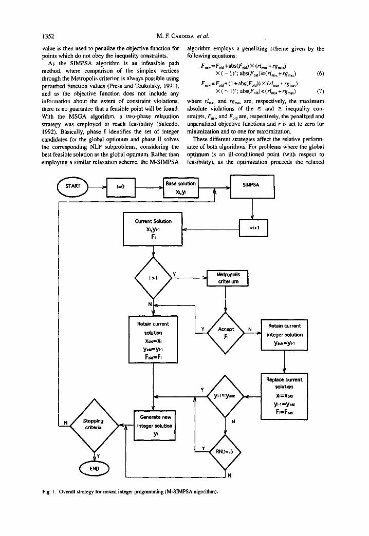
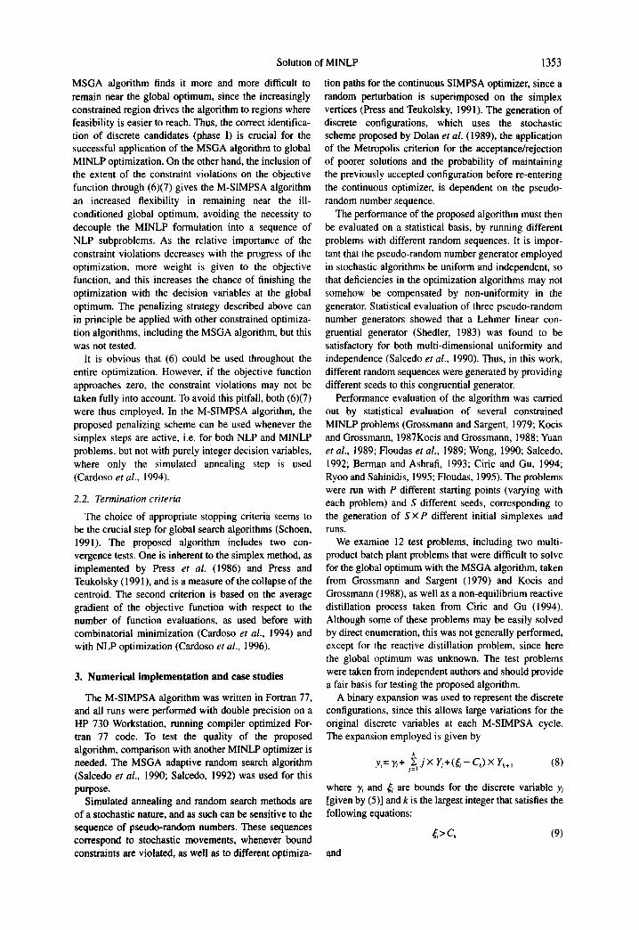
The M-SIMPSA algorithm is shown schematically in Fig. I, Basically, some initial solution vector (x,y), either feasible or infeasible, is fed to the continuous SIMPSA optimizer. Each global iteration of the M-SIMPSA algorithm comprises one cycle of the continuous SIMPSA optimizer, followed by one comparison through the Metropolis criterion for the complete solution vectors. This comparison allows the selection of different discrete configurations. To increase the chance of escaping difficult local optima and of finding feasible
points, each cycle of the SIMPSA algorithm toggles between a search over the global intervals [given by (4)] and a search over compressed intervals (Cardoso et al.,
1996), following the cooling schedule. The same cooling schedule is employed for both the continuous and discrete variables, i.e. the same temperature is used for both types of variables. Each SIMPSA iteration (two per cycle) comprises a number of simplex iterations, given by (100 ×p21n), where p is the number of continuous decision variables and n the total number of degrees of freedom. The generating scheme proposed by Dolan et al. (1989) is employed each time a different set of discrete variables is needed, whereby a first random number chooses the discrete variable to be changed and a second one chooses if the change is to be upwards or downwards by one unit.
If the Metropolis criterion accepts the current solu- tion, the algorithm proceeds by updating the solution vector and generating a different discrete configuration before re-entering the continuous SIMPSA optimizer. Since the continuous optimizer only performs two global iterations for each set of discrete variables, the con- tinuous variables may not be able to converge if the set of discrete variables is always forced to change. Thus, if the current solution is rejected (according to the Metropolis criterion) with a discrete configuration differ- ent from the previous one, the algorithm provides a 50% probability, i.e. an unbiased chance for the previous configuration to re-enter unchanged a new cycle of the SIMPSA optimizer. On the other hand, if the discrete configurations are the same, a new discrete configuration is always enforced, thus decreasing the chance of convergence to local optima.
It should be noted that the M-SIMPSA algorithm is applicable to MINLP problems, as well as to NLP and to combinatorial minimization problems. With NLP prob- lems, only the SIMPSA steps become active. For combinatorial minimization, the algorithm reduces to a simulated annealing scheme, where enforcement of different discrete configurations becomes mandatory at every step. Also, by specifying a zero value for the control temperature, the algorithm reduces to the non- linear simplex of Nelder and Mead for the continuous variables and to a purely random search algorithm for the discrete variables.
2.1. Deal ing with non-l inear constraints
An essential feature of optimization algorithms appli- cable to chemical engineering problems is the capability of dealing effectively with non-linear constraints, namely of finding solutions on surfaces described by active constraints as well as finding feasible points with highly constrained non-convex functions. In the SIMPSA algorithm, points produced by the simplex movement that do not obey either bound or implicit constraints are substituted by randomly generated points centered on the current best vertex, through the use of an appropriate generating function (Cardoso et al., 1996). By repeated application of this function, it is guaranteed that the bound constraints are obeyed. A large constant
1352 M. F. CARDOSA et al.
value is then used to penalize the objective function for points which do not obey the inequality constraints.
As the SIMPSA algorithm is an infeasible path method, where comparison of the simplex vertices through the Metropolis criterion is always possible using perturbed function values (Press and Teukolsky, 1991), and as the objective function does not include any information about the extent of constraint violations, there is no guarantee that a feasible point will be found. With the MSGA algorithm, a two-phase relaxation strategy was employed to reach feasibility (Salcedo, 1992). Basically, phase I identifies the set of integer candidates for the global optimum and phase II solves the corresponding NLP subproblems, considering the best feasible solution as the global optimum. Rather than employing a similar relaxation scheme, the M-SIMPSA
algorithm employs a penalizing scheme given by the following equations:
Foe.= Fo~+(1 + abs(Fo,d)) x (rlma~+rgmaO X ( - l)r; abs(Fold)<(rlmax+rgmax) (7)
where rlma, and rgm~ are, respectively, the maximum absolute violations of the < and -> inequality con- straints, F,~w and Fo~ a are, respectively, the penalized and unpenalized objective functions and r is set to zero for minimization and to one for maximization.
These different strategies affect the relative perform- ance of both algorithms. For problems where the global optimum is an ill-conditioned point (with respect to feasibility), as the optimization proceeds the relaxed
,.o I _l"a" I I x,y I
J SIMPSA
N
Current Solution xl,yH
FI
Y
Retain current soluUon Xou=Xl
Fo~=F,
.• Generate new integer solution
yl
.J Metropolis I - I cdterium
Y
Y
N
t
N
Retain current integer solution
y,==y~l
Replace current solution XImXold
y~l=yo. Fi=Fo.
Fig. I. Overall strategy for mixed integer programming (M-SIMPSA algorithm).
Solution
MSGA algorithm finds it more and more difficult to remain near the global optimum, since the increasingly constrained region drives the algorithm to regions where feasibility is easier to reach. Thus, the correct identifica- tion of discrete candidates (phase I) is crucial for the successful application of the MSGA algorithm to global MINLP optimization. On the other hand, the inclusion of the extent of the constraint violations on the objective function through (6)(7) gives the M-SIMPSA algorithm an increased flexibility in remaining near the ill- conditioned global optimum, avoiding the necessity to decouple the MINLP formulation into a sequence of NLP subproblems. As the relative importance of the constraint violations decreases with the progress of the optimization, more weight is given to the objective function, and this increases the chance of finishing the optimization with the decision variables at the global optimum. The penalizing strategy described above can in principle be applied with other constrained optimiza- tion algorithms, including the MSGA algorithm, but this was not tested.
It is obvious that (6) could be used throughout the entire optimization. However, if the objective function approaches zero, the constraint violations may not be taken fully into account. To avoid this pitfall, both (6)(7) were thus employed. In the M-SIMPSA algorithm, the proposed penalizing scheme can be used whenever the simplex steps are active, i.e. for both NLP and MINLP problems, but not with purely integer decision variables, where only the simulated annealing step is used (Cardoso et al., 1994).
2.2. Terminat ion criteria
The choice of appropriate stopping criteria seems to be the crucial step for global search algorithms (Schoen, 1991). The proposed algorithm includes two con- vergence tests. One is inherent to the simplex method, as implemented by Press et al. (1986) and Press and Teukolsky (1991), and is a measure of the collapse of the centroid. The second criterion is based on the average gradient of the objective function with respect to the number of function evaluations, as used before with combinatorial minimization (Cardoso et al., 1994) and with NLP optimization (Cardoso et al., 1996).
3. Numerical implementation and case studies
The M-SIMPSA algorithm was written in Fortran 77, and all runs were performed with double precision on a HP 730 Workstation, running compiler optimized For- tran 77 code. To test the quality of the proposed algorithm, comparison with another MINLP optimizer is needed. The MSGA adaptive random search algorithm (Salcedo et al., 1990; Salcedo, 1992) was used for this purpose.
Simulated annealing and random search methods are of a stochastic nature, and as such can be sensitive to the sequence of pseudo-random numbers. These sequences correspond to stochastic movements, whenever bound constraints are violated, as well as to different optimiza-
of MINLP 1353
tion paths for the continuous SIMPSA optimizer, since a random perturbation is superimposed on the simplex vertices (Press and Teukolsky, 1991). The generation of discrete configurations, which uses the stochastic scheme proposed by Dolan et al. (1989), the application of the Metropolis criterion for the acceptance/rejection of poorer solutions and the probability of maintaining the previously accepted configuration before re-entering the continuous optimizer, is dependent on the pseudo- random number sequence.
The performance of the proposed algorithm must then be evaluated on a statistical basis, by running different problems with different random sequences. It is impor- tant that the pseudo-random number generator employed in stochastic algorithms be uniform and independent, so that deficiencies in the optimization algorithms may not somehow be compensated by non-uniformity in the generator. Statistical evaluation of three pseudo-random number generators showed that a Lehmer linear con- gruential generator (Shedler, 1983) was found to be satisfactory for both multi-dimensional uniformity and independence (Salcedo et al., 1990). Thus, in this work, different random sequences were generated by providing different seeds to this congruential generator.
Performance evaluation of the algorithm was carried out by statistical evaluation of several constrained MINLP problems (Grossmann and Sargent, 1979; Kocis and Grossmann, 1987Kocis and Grossmann, 1988; Yuan et al., 1989; Floudas et al., 1989; Wong, 1990; Salcedo, 1992; Berman and Ashrafi, 1993; Ciric and Gu, 1994; Ryoo and Sahinidis, 1995; Floudas, 1995). The problems were run with P different starting points (varying with each problem) and S different seeds, corresponding to the generation of S × P different initial simplexes and r u n s .
We examine 12 test problems, including two multi- product batch plant problems that were difficult to solve for the global optimum with the MSGA algorithm, taken from Grossmann and Sargent (1979) and Kocis and Grossmann (1988), as well as a non-equilibrium reactive distillation process taken from Ciric and Gu (1994). Although some of these problems may be easily solved by direct enumeration, this was not generally performed, except for the reactive distillation problem, since here the global optimum was unknown. The test problems were taken from independent authors and should provide a fair basis for testing the proposed algorithm.
A binary expansion was used to represent the discrete configurations, since this allows large variations for the original discrete variables at each M-SIMPSA cycle. The expansion employed is given by
k yi=Yi+j~=,j×Yj+(~i-C~)XYk÷, ( 8 )
where "yj and ~ are bounds for the discrete variable Yl [given by (5)] and k is the largest integer that satisfies the following equations:
where the Yj are binary variables. Other more or less equivalent transformations are possible (Floudas, 1995).
For all MINLP problems the error criterion was set at 10 -s, for both the convergence of the simplex algorithm (as given by Press and Teukolsky, 1991) and for convergence of the smoothed function values, and the cooling schedule parameter was set at 10-2 (Cardoso et al., 1996). For purely discrete decision variables (exam- ples 4, 6 and 8), the error criterion was set at 10 -3 and the cooling schedule parameter was set at 10 (Cardoso et al., 1994). For all problems, the initial search regions were determined from the bound constraints. Table 1 gives a brief summary of the test problems, where the first nine problems were solved with the M-SIMPSA algorithm starting from 100 randomly generated initial simplexes, i.e. 100 different random number sequences.
As the bounds of the decision variables are automat- ically searched for in both the M-SIMPSA and MSGA algorithms, the global optimum may be found irrespec- tive of the effectiveness of the random search or simulated annealing/simplex approaches. Thus, the test on the extremes was deactivated in both algorithms for all problems to provide a correct appraisal of their reliability.
4 . R e s u l t s a n d d i s c u s s i o n
Example 1. This example is taken from Kocis and Grossmann (1988) and is also given in Floudas et al. (1989) and Ryoo and Sahinidis (1995):
rain 2x+y
s.t.
1 .25 - x 2 - y--<0
x + y ~ l . 6
0--<x~ 1.6
y={O,l )
where non-convexities arise in the first constraint. There is a local optimum at {x,y;F} = {I.118,0;2.236} which
M. E CARDOSA et al.
was obtained in a single run. The global optimum {x,y;F} = {0.5,1;2} was found in the remaining 99 runs with, on average, 607 function evaluations and 0.048 s per run. With the penalizing scheme, the global optimum was always found, with 16,282 function evaluations and 0.57 s per run.
Example 2. This example is taken from Kocis and Grossmann (1987) and is also given in Salcedo (1992):
min - y+2x~ +x~
s.t.
xl - 2 exp( - x2)=0
- xt +x2+y<--O
0.5-<x~ <-- 1.4
y={0,1}
The global optimum {x~,x2,y;F} = { 1.375,0.375,1 ;2.124 } was found 83% of the time without the penalizing scheme with, on average, 10,528 function evaluations and 0.29 s per run. With the penalizing scheme, the successes increased to 100%, with 14,440 function evaluations and 0.57 s per run.
Example 3. This example is taken from Fioudas (1995):
min - 0.7y+5(xt - 0.5)2+0.8
s.t.
- exp(x) - 0.2) - x2-<0
x2+ l . l y - < - 1
xt - 1.2y'~0.2
0.2-~xt-<l
- 2 .22554-x2- < - 1
y={0,1}
and is non-convex because of the first constraint. The global optimum {x~,x2,y;F} = { 0.94194, - 2.1,1; 1.07654 } was found 100% of the time, but only with the penalizing scheme with, on average, 38,042 function evaluations and 1.784 s per run. Without the penalizing scheme, all solutions were infeasible.
Example 4. This example is taken from Kocis and Grossmann (1988), and is also given in Floudas et al. (1989), Salcedo (1992) and Ryoo and Sahinidis (1995):
min 2x~ +3x2+ 1.5y t +2y 2 - 0.5y3
s.t.
x~+y~=l.25
x ~ + 1.5y2=3.00
x t +y~-< 1.60
1.333x2 +y2-----3.00
-y~ -y2+y~<-O x~,x2 >--O y={0,1} 3
This problem is non-convex because of the equality constraints (Floudas et al., 1989). The global optimum {yj,yvy3;F}={O,l,1;7.667180} was always found with {Y~,Y2,Y3} as decision variables with, on average, 577 function evaluations and 0.08 s per run.
Example 5. This example, taken from Kocis and
Solution of MINLP
Grossmann (1989) and also given in Diwekar et al.
(1992) and Diwekar and Rubin (1993), is a two-reactor problem, where selection is to be made among two candidate reactors for minimizing the cost of producing a desired product:
min 7.5y~ +5.5y2+7v~ +6v2+5x
s.t.
yl+y_,= 1
zt =0.911 - exp( - 0.5 vl)]x I
z2 =0.811 - exp( - 0.4v,)]x2
X I "l-X 2 - - X = 0
z~ +z,= 10 s.t. v,<--lOy,
v2<-- 10y2
x,<_2Oy,
x2<--20y,
XI.,X2,Zl,Z2,Vl,V2~O y={0,1} 2
The global optimum {y2,z2,v,v2;F} =
{ 0,0,3.514237,0;99.2396 } was always found without the penalizing scheme with, on average, 14,738 function evaluations and 0.77 s per run. With the penalizing scheme, these increased, respectively, to 42,295 function evaluations and 2.47 s per run.
Example 6. This example represents a quadratic capital budgeting problem, taken from Kocis and Grossmann (1988) and also given in Salcedo (1992), and has four binary variables and features bilinear terms in the objective function:
The global optimum { Y~,Yz,Y3,y4;F} = { 0,0,1,1 ; - 6 } was always found with, on average, 4477 function evalua- s.t. tions and 0.30 s per run.
Example 7. This example is taken from Yuan et al.
(1989), and is also given in Floudas et al. (1989), Salcedo (1992) and Ryoo and Sahinidis (1995):
min (Yt- 1)2+(Y2- 2)2+(Y3- 1) 2 - In(y4+ l ) + ( x l - 1) 2 +(x, - 2) ~" + (x~ - 3) 2
s.t.
Y, +Y,. +Y3 +x, +x 2 +x3<-5 y~+x~+x~+x~<-5.5
Yl +xE <- 1.2
Y2 +Xz <- 1.8
y3+x3-2.5
y4+x~-l .2
y~+x~<-l.64
y~+x~<-4.25
y~+x]<-4.64
x>0 y={0,1} 4
1355
This problem features non-linearities in both continuous and binary variables and has seven degrees of freedom. The global optimum {x,,x2,x3,y,,y,.,y.~,y4;F} =
{0.2,0.8,1.907878,1,1,0,1 ;4.579582} was found 60% of the time without the penalizing scheme with, on average, 22,309 function evaluations and 1.28 s per run. With the penalizing scheme, the global optimum was obtained 97% of the time, with 63,751 function evaluations and 4.40 s per run.
Example 8. This example is taken from Berman and Ashrafi (1993):
The global optimum {y;F}={0,1.1,1,0,1,1,0;0.93634} was always found, with 15,462 function evaluations and 1.52 s per run.
It is interesting to note that, by solving this problem assuming the decision variables to be continuous, the global optimum becomes {x,F}={0.08346,1,0.9869, 0.9118,0,0.9985,0.3532,0.9911 ;0.940785 } which, when rounded to the nearest integer values, becomes { y;F} = { 0,1,1,1,0,1,0,1 ;0.898123 }, which is feasible but does not correspond to the global optimum.
Example 9. This example is taken from Wong (1990):
max - 5.357854x~ - 0.835689ylx3 - 37.29329yl + 40792.141
s f =a l + az.v2x 3 + a.ay lx2 -- a4xlx3
s2=as +aayrx3 +aTy&2 +asx ~ -- 90
s3=ag +a~ox~x3 +aHy~xj +a~2x~x2 -- 20
s,<--92
s2-<20
s3-<5
78<y~<102
33<y2<45
27<x~,x2,x3<45 y={0,1} 2
The global optimum corresponds to {y~,x~,x.~;F}=
{78,27,27;32217.4} and was obtained with various different feasible combinations of {y2,x2}. It was found 87% of the time without the penalizing scheme, with 27,410 function evaluations and 4.19 s per run, and 95% of the time with the penalizing scheme, with 33,956 function evaluations and 6.06 s per run.
Table 2 gives a summary of the reliability of the M-
CAC£ 21:12-B
1356 M. E CARDOSA etal.
Table 2. Brief summary of test results (number of successes in obtaining the global optimum out of 100 runs)
Example M-SIMPSA MSGA Without penalizing Penalizing
SIMPSA algorithm for example problems 1-9, where it may be stated that the algorithm is generally robust and reliable. In some MINLP cases, however, the algorithm only attains feasible solutions and the global optimum with the penalizing scheme. This occurs at some expense in CPU time, on the average roughly doubling it, but the increased reliability in obtaining the global optimum justifies it. By comparison, the adaptive MSGA algo- rithm is extremely reliable for these small-scale prob- lems, where the global optimum was, in practice, always obtained for all problems. We will see below, however, that for larger scale and more demanding problems the M-SIMPSA algorithm behaves better than the MSGA algorithm.
Examples 10/11 (multi-product batch plant). The multi-product batch plant consists of M processing stages in series where fixed amounts Q~ of N products have to be manufactured. The objective is to determine for each stage j the number of parallel units N s and their sizes V s and for each product i the corresponding batch sizes B~ and cycle times TL~. The problem data are the horizon time H, the size factors S 0 and processing times t o of product i in stage j, the required productions Q~, and appropriate cost functions a s and fls' The mathematical formulation of this problem is as follows (Grossmann and Sargent, 1979; Kocis and Grossmann, 1988):
M
min E tr/vjv~J
S.t.
i=1
vj>_s,~, NjTLi>-tlj I~Nj~Ny
TLi~ TLi-- TL~ I~ ~ u B j - B j - B s
Nj integer
The upper (u) and lower (I) bounds N~, V~, V~ are specified by the problem and appropriate bounds for TL~ and B~ can be determined as follows:
TL,=max tU Ny ~LI = max jt U
Q,
The optimization of a multi-product batch plant with data structure as formulated has 2(M+N) degrees of freedom, 4(M+N) bound constraints, 1 (<) and 2MN (->) inequality constraints. The objective function, the horizon time constraint and several inequalities are non- convex. Thus, depending on the values of M and N, a fairly large non-convex MINLP problem may result. Non-convexities in this problem may easily be elimi- nated using logarithmic transformations, and this was actually done by Kocis and Grossmann (1988) to good advantage in testing their MINLP algorithm. The possible number of parallel units for each stage ~ as well as the number of stages M will determine the number of NLP subproblems embedded in the original MINLP formulation. We examine below two cases of increasing complexity, where the relevant data is given in Table 3. Both cases were run with 10 random starting points and 100 different seeds, corresponding to 1000 runs per case.
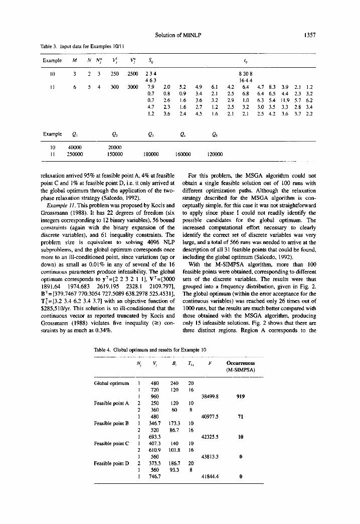
Example 10. This problem, proposed by Grossmann and Sargent (1979), has 10 degrees of freedom (three integers corresponding to six binary variables), 26 bound constraints (with the binary expansion of the discrete variables), and 13 inequality constraints. The problem size is equivalent to solving 27 NLP subproblems, and the global optimum, with respect to feasibility, corre- sponds to an extremely ill-conditioned point. With linear programming problems, the optimum, when unique, lies in the intersection of two or more constraints. Hence, moving slightly away from it (in the wrong direction) will certainly lead to infeasibility. In this non-linear example, variations in any direction (up or down) as small as 0.01% in any of the seven continuous parameters produces infeasibility, and this is not a characteristic feature of optimum solutions of non-linear optimization problems.
By direct application of the MSGA algorithm, the global optimum was never obtained, although feasible points were always obtained. However, phase I of the relaxed MSGA algorithm was capable of identifying the global optimum in all cases, albeit at a greater expense in computational effort (Salcedo, 1992).
Table 4 gives the results obtained with the M- SIMPSA algorithm in solving this example. It shows that the global optimum was reached 919 times out of I000 runs, starting always from infeasible points (that obey the bound constraints but not the inequality constraints). The average number of function evalua- tions was 257,536, against 35,000 with the MSGA algorithm. However, the MSGA algorithm without
relaxation arrived 95% at feasible point A, 4% at feasible point C and 1% at feasible point D, i.e. it only arrived at the global optimum through the application of the two- phase relaxation strategy (Salcedo, 1992).
Example l I . This problem was proposed by Kocis and Grossmann (1988). It has 22 degrees of freedom (six integers corresponding to 12 binary variables), 56 bound constraints (again with the binary expansion of the discrete variables), and 61 inequality constraints. The problem size is equivalent to solving 4096 NLP subproblems, and the global optimum corresponds once more to an ill-conditioned point, since variations (up or down) as small as 0.01% in any of several of the 16 continuous parameters produce infeasibility. The global optimum corresponds to yT=[2 2 3 2 l l], VT=[3000 1891.64 1974.683 2619.195 2328.1 2109.797], B T = [379.7467 770.3054 727.5089 638.2978 525.4531 ], T~=[3.2 3.4 6.2 3.4 3.7] with an objective function of $285,510/yr. This solution is so ill-conditioned that the continuous vector as reported truncated by Kocis and Grossmann (1988) violates five inequality (->) con- straints by as much as 0.34%.
For this problem, the MSGA algorithm could not obtain a single feasible solution out of 100 runs with different optimization paths. Although the relaxation strategy described for the MSGA algorithm is con- ceptually simple, for this case it was not straightforward to apply since phase I could not readily identify the possible candidates for the global optimum. The increased computational effort necessary to clearly identify the correct set of discrete variables was very large, and a total of 566 runs was needed to arrive at the description of all 31 feasible points that could be found, including the global optimum (Saicedo, 1992).
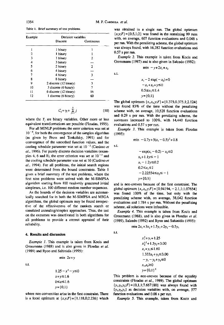
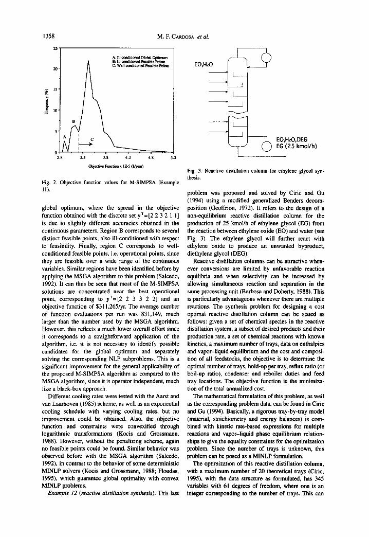
With the M-SIMPSA algorithm, more than 100 feasible points were obtained, corresponding to different sets of the discrete variables. The results were thus grouped into a frequency distribution, given in Fig. 2. The global optimum (within the error acceptance for the continuous variables) was reached only 26 times out of 1000 runs, but the results are much better compared with those obtained with the MSGA algorithm, producing only 15 infeasible solutions. Fig. 2 shows that there are three distinct regions. Region A corresponds to the
Table 4. Global optimum and results for Example 10
Nj Vj B i T u F Occurrences (M-SIMPSA)
Global optimum 1 480 240 20 1 720 120 16 l 960 38499.8 919
Feasible point A 2 250 120 l0 2 360 60 8 1 480 40977.5 71
Feasible point B 1 346 .7 173.3 10 2 520 86.7 16 1 693.3 42325.5 10
Feasible point C l 407.3 140 l0 2 610 .9 101.8 16 1 560 43813.3 0
Feasible point D 2 373 .3 186.7 20 I 560 93.3 8 I 746.7 41844.4 0
1358
25'
20'
15'
i 10'
M. E CARDOSA et al.
O 2.8 5.3
A: m-comlitiotted Global Optimum A B: lll-¢andititm~ F.casi hie Points
Feasible Points
• • i , . ° . , . , .
3.3 3.8 4.3 4,8
Obj~-tivc Function x IE-5 (S/year)
EO,HzO
Fig. 2. Objective function values for M-SIMPSA (Example I1).
global optimum, where the spread in the objective function obtained with the discrete set yr=[2 2 3 2 1 1] is due to slightly different accuracies obtained in the continuous parameters. Region B corresponds to several distinct feasible points, also ill-conditioned with respect to feasibility. Finally, region C corresponds to well- conditioned feasible points, i.e. operational points, since they are feasible over a wide range of the continuous variables. Similar regions have been identified before by applying the MSGA algorithm to this problem (Salcedo, 1992). It can thus be seen that most of the M-SIMPSA solutions are concentrated near the best operational point, corresponding to yT=[2 2 3 3 2 2] and an objective function of $311,265/yr. The average number of function evaluations per run was 831,149, much larger than the number used by the MSGA algorithm. However, this reflects a much lower overall effort since it corresponds to a straightforward application of the algorithm, i.e. it is not necessary to identify possible candidates for the global optimum and separately solving the corresponding NLP subproblems. This is a significant improvement for the general applicability of the proposed M-SIMPSA algorithm as compared to the MSGA algorithm, since it is operator independent, much like a black-box approach.
Different cooling rates were tested with the Aarst and van Laarhoven (1985) scheme, as well as an exponential cooling schedule with varying cooling rates, but no improvement could be obtained. Also, the objective function and constraints were convexified through logarithmic transformations (Kocis and Grossmann, 1988). However, without the penalizing scheme, again no feasible points could be found. Similar behavior was observed before with the MSGA algorithm (Salcedo, 1992), in contrast to the behavior of some deterministic MINLP solvers (Kocis and Grossmann, 1988; Floudas, 1995), which guarantee global optimality with convex MINLP problems.
Example 12 (reactive distillation synthesis). This last
I f
-'1 I
~ EO,HzO,DEG EG (25 kmol/h)
Fig. 3. Reactive distillation column for ethylene glycol syn- thesis.
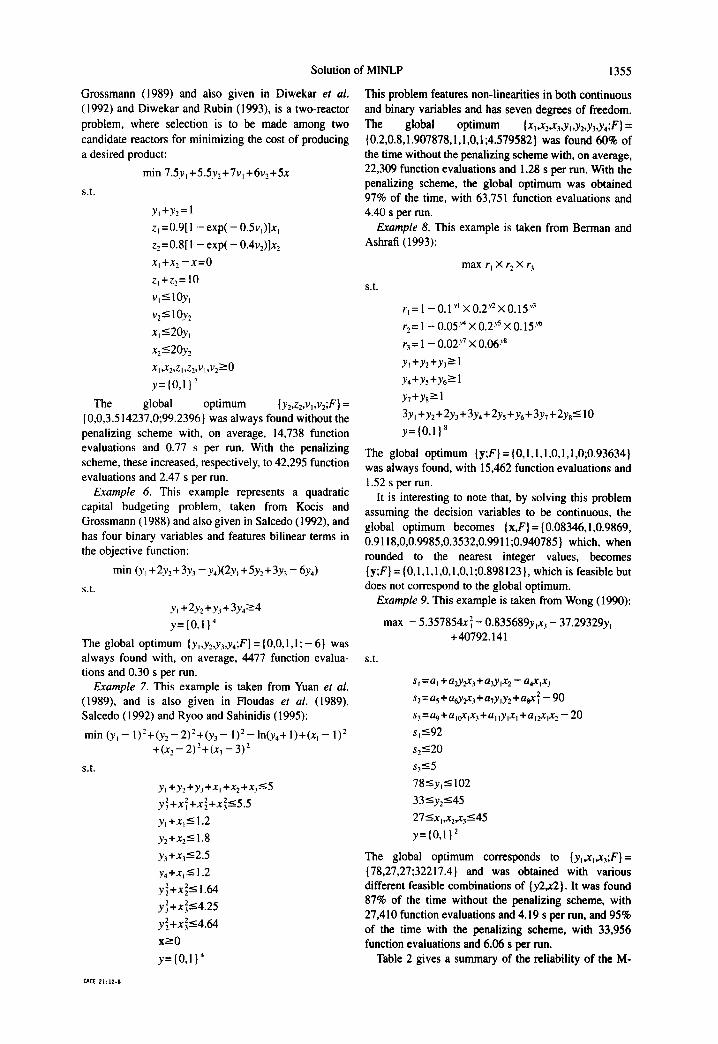
problem was proposed and solved by Ciric and Gu (1994) using a modified generalized Benders decom- position (Geoffrion, 1972). It refers to the design of a non-equilibrium reactive distillation column for the production of 25 kmol/h of ethylene glycol (EG) from the reaction between ethylene oxide (EO) and water (see Fig. 3). The ethylene glycol will further react with ethylene oxide to produce an unwanted byproduct, diethylene glycol (DEG).
Reactive distillation columns can be attractive when- ever conversions are limited by unfavorable reaction equilibria and when selectivity can be increased by allowing simultaneous reaction and separation in the same processing unit (Barbosa and Doherty, 1988). This is particularly advantageous whenever there are multiple reactions. The synthesis problem for designing a cost optimal reactive distillation column can be stated as follows: given a set of chemical species in the reactive distillation system, a subset of desired products and their production rate, a set of chemical reactions with known kinetics, a maximum number of trays, data on enthalpies and vapor-liquid equilibrium and the cost and composi- tion of all feedstocks, the objective is to determine the optimal number of trays, hold-up per tray, reflux ratio (or boil-up ratio), condenser and reboiler duties and feed tray locations. The objective function is the minimiza- tion of the total annualized cost.
The mathematical formulation of this problem, as well as the corresponding problem data, can be found in Ciric and Gu (1994). Basically, a rigorous tray-by-tray model (material, stoichiometry and energy balances) is com- bined with kinetic rate-based expressions for multiple reactions and vapor-liquid phase equilibrium relation- ships to give the equality constraints for the optimization problem. Since the number of trays is unknown, this problem can be posed as a MINLP formulation.
The optimization of this reactive distillation column, with a maximum number of 20 theoretical trays (Ciric, 1995), with the data structure as formulated, has 345 variables with 61 degrees of freedom, where one is an integer corresponding to the number of trays. This can
Solution
be considered as a fairly large highly non-linear non- convex problem, since the material balances contain bi- and trilinear terms and the reaction rate terms, vapor- liquid equilibria evaluations and objective function are highly non-linear. This problem can be solved as a succession of up to 20 NLP subproblems simply by direct enumeration of the number of theoretical trays. This was eventually performed in order to determine the global optimum, since it was unknown.
With the M-SIMPSA algorithm, the starting sim- plexes were generated from random initial solution vectors of both the continuous and discrete variables, i.e. mostly from infeasible points. Ciric and Gu (1994) state that the generalized Benders decomposition simply requires selecting an initial solution vector of the discrete variables, i.e. the number of theoretical trays. However, an initial feasible set of continuous variables seems to be quite helpful for solving this particular problem, and the procedure proposed by these authors is more efficient when starting with a single tray column. Such information does not seem to be helpful with the M-SIMPSA algorithm, since this algorithm initially accepts poorer solutions with a high probability, quickly departing from the initial point to search the variable space.
Ciric and Gu (1994) have found that the best solution corresponds to 10 theoretical trays, with a total cost of
of MINLP 1359
$15.69× 10⁶/yr. These authors have used additional constraints on maximum molar flow rates of 1000 kmol/ h (Ciric, 1995). We have simulated their solution and found very similar results, including temperature and composition profiles. However, optimization with the M-SIMPSA algorithm including the above constraints produced an objective function of $15.40 × 10⁶/yr, also corresponding to 10 trays but to totally different feed tray locations and hold-up ratios.
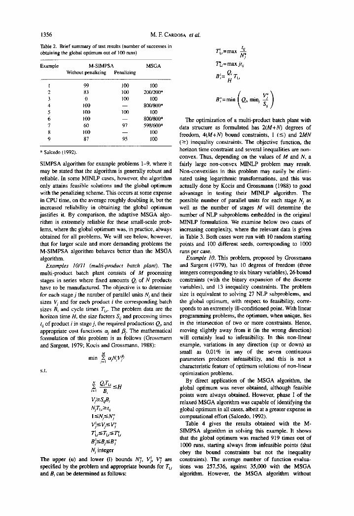
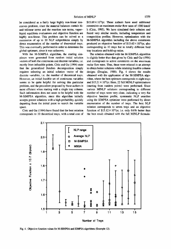
The solution obtained with the M-SIMPSA algorithm is slightly better than that given by Ciric and Gu (1994) and corresponds to active constraints on the maximum molar flow rates. Thus, these were relaxed in an attempt to obtain better solutions while retaining feasible column designs (Douglas, 1988). Fig. 4 shows the results obtained with the application of the M-SIMPSA algo- rithm, where the best optimum corresponds to eight trays and $15.21 × 10⁶/yr. Here, 22 full MINLP optimizations (starting from random points) were performed. Since various MINLP solutions corresponding to different number of trays were very close, indicating a very fiat objective function profile, systematic NLP searches using the SIMPSA optimizer were performed by direct enumeration of the number of trays. The best NLP solution corresponds to seven trays and an objective function of $15.12× 10⁶/yr, i.e. only 0.6% better than the best result obtained with the full MINLP formula-
A i , _ e~
X
t - O
:3 LL ¢J .> "6 4)
2.1
20 I 1.9'
1.8'
1.7'
1.6'
1.5
" NLP range
O Average NLP
[] M-SIMPSA
• MSGA
O @
@
s° I I I ' 3 5 11 13
D
O
D
i i
|
15
Number of Trays
Fig. 4. Objective function values for M-SIMPSA and SIMPSA algorithms (Example 12).
1360
tion. This figure also shows the results obtained with the MSGA algorithm (14 runs) where the best result corresponding to $15.26× 10⁶/yr is very close to the best obtained with the M-SIMPSA algorithm. However, most results are poorer than those obtained with the proposed algorithm.
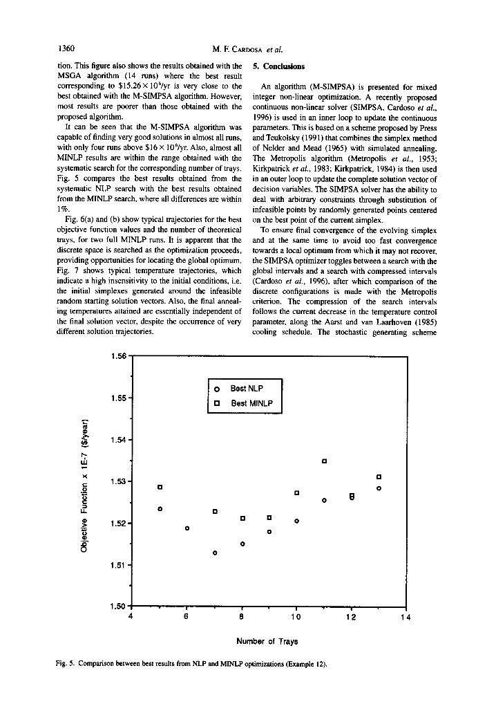
It can be seen that the M-SIMPSA algorithm was capable of finding very good solutions in almost all runs, with only four runs above $16 × 106/yr. Also, almost all MINLP results are within the range obtained with the systematic search for the corresponding number of trays. Fig. 5 compares the best results obtained from the systematic NLP search with the best results obtained from the MINLP search, where all differences are within 1%.
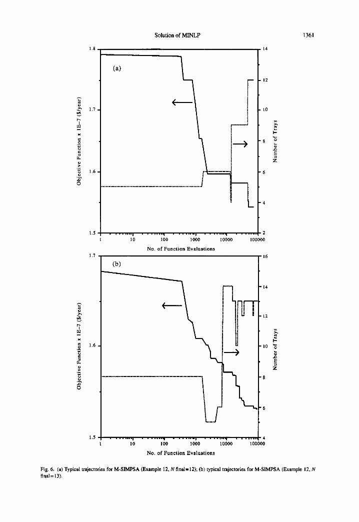
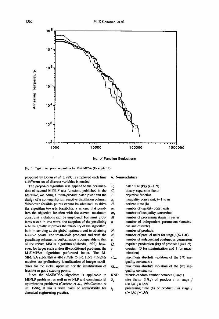
Fig. 6(a) and (b) show typical trajectories for the best objective function values and the number of theoretical trays, for two full MINLP runs. It is apparent that the discrete space is searched as the optimization proceeds, providing opportunities for locating the global optimum. Fig. 7 shows typical temperature trajectories, which indicate a high insensitivity to the initial conditions, i.e. the initial simplexes generated around the infeasible random starting solution vectors. Also, the final anneal- ing temperatures attained are essentially independent of the final solution vector, despite the occurrence of very different solution trajectories.
M. E CARDOSA et al.
5. Conclusions
An algorithm (M-SIMPSA) is presented for mixed integer non-linear optimization. A recently proposed continuous non-linear solver (SIMPSA, Cardoso et al. ,
1996) is used in an inner loop to update the continuous parameters. This is based on a scheme proposed by Press and Teukolsky (1991) that combines the simplex method of Nelder and Mead (1965) with simulated annealing. The Metropolis algorithm (Metropolis et al., 1953; Kirkpatrick et al., 1983; Kirkpatrick, 1984) is then used in an outer loop to update the complete solution vector of decision variables. The SIMPSA solver has the ability to deal with arbitrary constraints through substitution of infeasible points by randomly generated points centered on the best point of the current simplex.
To ensure final convergence of the evolving simplex and at the same time to avoid too fast convergence towards a local optimum from which it may not recover, the SIMPSA optimizer toggles between a search with the global intervals and a search with compressed intervals (Cardoso et al., 1996), after which comparison of the discrete configurations is made with the Metropolis criterion. The compression of the search intervals follows the current decrease in the temperature control parameter, along the Aarst and van Laarhoven (1985) cooling schedule. The stochastic generating scheme
1.56
1 .55 '
A t . ,
1.54,
X
,.. 1.53' 0
0 C
0 .> 1.52'
II) ° ~ . D
O
1.51
1.50
o
o
o
I 0 Best NLP I 0 Best MINLP
El [] []
0
0 0
0
o B
! ! ! |
4 6 8 10 12
O O
Number of Trays
Fig. 5. Comparison between best results from NLP and MINLP optimizations (Example 12).
Fig. 6. (a) Typical trajectories for M-SIMPSA (Example 12, N final= 12); (b) typical trajectories for M-SIMPSA (Example 12, N final= 13).
1362 M. E CARDOSA et al.
10 8
10 7,
10 6 , P _= $ ® Q.
E 10 5 . I - o~ ._c
¢-
c 10 4. <
10 3
l O 2 - 1 - 1000 10000 100000 1 0 0 0 0 0 0
No. o1 Function Evaluations
Fig. 7. Typical temperature profiles for M-SIMPSA (Example 12).
proposed by Dolan et al. (1989) is employed each time a different set of discrete variables is needed.
The proposed algorithm was applied to the optimiza- B i tion of several MINLP test functions published in the Ck literature, including a multi-product batch plant and the F design of a non-equilibrium reactive distillation column, gj Whenever feasible points cannot be obtained, to drive H the algorithm towards feasibility, a scheme that penal- m~ izes the objective function with the current maximum m s constraint violations can be employed. For most prob- M lems tested in this work, the adoption of the penalizing n scheme greatly improves the reliability of the algorithm, both in arriving at the global optimum and in obtaining N feasible points. For small-scale problems and with the Nj penalizing scheme, its performance is comparable to that p of the robust MSGA algorithm (Salcedo, 1992); how- Qi ever, for larger scale and/or ill-conditioned problems, the r M-SIMPSA algorithm performed better. The M- SIMPSA algorithm is also simple to use, since it neither r/.= requires the preliminary identification of integer candi- dates for the global optimum nor the identification of rg,,~ feasible or good starting points.
Since the M-SIMPSA algorithm is applicable to RND MINLP problems, as well as to NLP and combinatorial S U optimization problems (Cardoso et al., 1994Cardoso et al., 1996), it has a wide basis of applicability for t 0 chemical engineering practice.
6. Nomenclature
batch size (kg) (i= I,N) binary expansion factor objective function inequality constraint, j = 1 to m horizon time (h) number of equality constraints number of inequality constraints number of processing stages in series number of independent parameters (continu- ous and discrete) number of products number of parallel units for stage j (j= I,M) number of independent continuous parameters required production (kg) of product i (i= 1,N) constant (0 for minimization and I for maxi- mization) maximum absolute violation of the ( - ) ine- quality constraints maximum absolute violation of the (-->) ine- quality constraints pseudo-random number between 0 and 1 size factor (l/kg) of product i in stage j (i= I,N; j = I ,M) processing time (h) of product i in stage j ( i f 1,N; j = I,M)
Solution of MINLP 1363
TLi v,.
X
Y Yaux
Y i - I
Yota
E
cycle time (h) of product i (i= I,N) capacity (i) of parallel unit in processing stage j (j= I,M) continuous decision vector discrete decision vector discrete variable temporarily retained for com- parison purposes discrete variable input to the SIMPSA algo- rithm current value for discrete variable binary variable
Greek letters ai lower bound on continuous parameter x i
(i = t,p) aj cost coefficient ($) of stage j (]= 1,M) fll upper bound on continuous parameter x~
(i = I,p) flj cost coefficient (dimensionless) of stage j
(j= I,M) y~ lower bound on discrete parameter Yi (i= l,n-
This work was partially supported by JNICT (Portu- guese Junta Nacional de InvestigagAo Cientffica e Tecnol6gica), under Contract No. BD/1457/91-RM, and PRAXIS XXI, under Contract No. BD/3236/94, employ- ing the computational facilities of Instituto de Sistemas e Robttica (ISR), Porto. The authors thank Dr. J. Bastos for providing crucial parts of the code needed to simulate the distillation process.
References
Aarst, E., and Korst, J. (1989) Simulated Annealing and Boltzmann Machines - A Stochastic Approach to Combinatorial Optimization and Neural Com- puters. Wiley, New York.
Aarst, E. H. L. and van Laarhoven, P. J. M. (1985) Statistical cooling: a general approach to combina- torial optimization problems. Philips J. Res. 40, 193
Barbosa, D. and Doherty, M. E (1988) The influence of equilibrium chemical reactions on vapor-liquid phase diagrams. Chem. Eng. Sci. 43(3), 529
Berman, O. and Ashrafi, N. (1993) Optimization models for reliability of modular software systems. IEEE Trans. Soft. Eng. 19, 1119
Campbell, J. R. and Gaddy, J. L. (1976) Methodology
for simultaneous optimization with reliability: nuclear PWR example. AIChE J. 22(6), 1050
Cardoso, M. E, Salcedo, R. L. and de Azevedo, S. E (1994) Non-equilibrium simulated annealing: a faster approach to combinatorial minimization. Ind. Eng. Chem. Res. 33(8), 1908
Cardoso, M. E, Salcedo, R. L. and de Azevedo, S. E (1996) The simplex-simulated annealing approach to continuous non-linear optimization. Comput. Chem. Eng. 20(9), 1065
Ciric, A. R. (1995) Personal communication. Ciric, A. R. and Gu, D. (1994) Synthesis of non-
equilibrium reactive distillation processes by MINLP optimization. AIChE. J. 40(9), 1479
Das, H., Cummings, P. T. and Levan, M. D. (1990) Scheduling of serial multiproduct batch processes via simulated annealing. Comput. Chem. Eng. 14(12), 1351
Diwekar, U. M., Grossmann, I. E. and Rubin, E. S. (1992) An MINLP process synthesizer for a sequential modular simulator. Ind. Eng. Chem. Res. 31(1), 313
Diwekar, U. M. and Rubin, E. S. (1993) Efficient handling of the implicit constraints problem for the ASPEN MINLP synthesizer. Ind. Eng. Chem. Res. 32(9), 2006
Dolan, W. B., Cummings, P. T. and Levan, M. D. (1989) Process optimization via simulated annealing: application to network design. AIChE. J. 35(5), 725
Douglas, G. M. (1988) Conceptual Design of Chemical Processes. McGraw-Hill, New York.
Duran, M. A. and Grossmann, I. E. (1986) A mixed integer nonlinear programming approach for proc- ess synthesis. AIChE. J. 32(4), 592
Fioudas, C. A. and Ciric, A. R. (1989) Strategies for overcoming uncertainties in heat-exchanger net- work synthesis. Comput. Chem. Eng. 13(10), 1133
Floudas, C. A., Aggarwal, A. and Ciric, A. R. (1989) Global optimum search for nonconvex NLP and MINLP problems. Comput. Chem. Eng. 13(10), I l l7
FIoudas, C. A. (1995) Nonlinear and Mixed-Integer Optimization - Fundamentals and Applications. Oxford University Press, Oxford.
Geoffrion, A. M. (1972) Generalized Benders decom- position. J. Opt. Theory Appl. 10(4), 237
Grossmann, I. E. and Daichendt, M. M. (1994) New trends in optimization-based approaches to process synthesis. In Proc. PSE '94, Fifth Int. Syrup. on Process Systems Engineering, edited by En Sup Yoon. Korean Institute of Chemical Engineers, Kyongju, Korea, p. 95.
Grossmann, I. E. and Kravanja, Z. (1995) Mixed-integer nonlinear programming techniques for process systems engineering. Comput. Chem. Eng. 19(Suppl.), S189
Grossmann, I. E. and Sargent, R. W. H. (1979) Optimal design of multipurpose chemical plants. Ind. Eng. Chem. Process Des. Dev. 18, 343
Kirkpatrick, S. (1984) Optimization by simulated annealing: quantitative studies. J. Stat. Phys. 34(5/6), 975
Kirkpatrick, S., Gelatt, C. D. and Vechi, M. P. (1983) Optimization by simulated annealing. Science 220, 671
1364 M. E CARDOSA et al.
Kocis, G. R. and Grossmann, I. E. (1987) Relaxation strategy for the structural optimization of process flowsheets. Ind. Eng. Chem. Res. 26, 1869
Kocis, G. R. and Grossmann, I. E. (1988) Global optimization of nonconvex mixed-integer nonlinear programming (MINLP) problems in process syn- thesis. Ind. Eng. Chem. Res. 27, 1407
Kocis, G. R. and Grossmann, I. E. (1989) A modeling and decomposition strategy for MINLP optimiza- tion of process flowsheets. Comput. Chem. Eng. 13, 797
Mangasarian, O. L. (1994) Nonlinear Programming. SIAM, Philadelphia, PA, p. 42.
Metropolis, N., Rosenbluth, A., Rosenbluth, M., Teller, A. and Teller, E. (1953) Equation of state calcula- tions by fast computing machines. J. Chem. Phys. 21, 1087
Nelder, J. A. and Mead, R. (1965)A simplex method for function minimization. Comput. J. 7, 308
Ostrovsky, G. M., Ostrovsky, M. G. and Mikhailow, G. W. (1990) Discrete optimization of chemical proc- esses. Comput. Chem. Eng. 14(1), I!1
Patel, A. N., Mah, R. S. H. and Karimi, I. A. (1991) Preliminary design of multiproduct noncontinuous plants using simulated annealing. Comput. Chem. Eng. 15(7), 451
Press, W. H. and Teukolsky, S. A. (1991) Simulated annealing optimization over continuous spaces. Comput. Phys. 5(4), 426
Press, W. H., Flannery, B. P., Teukolsky, S. A. and
Vetteding, W. T. (1986) Numerical Recipes: The Art of Scientific Computing. Cambridge University Press, New York.
Ryoo, H. S. and Sahinidis, N. V. (1995) Global optimization of nonconvex NLPs and MINLPs with applications in process design. Comput. Chem. Eng. 19(5), 551
Salcedo, R., Gongalves, M. J. and de Azevedo, S. E (1990) An improved random-search algorithm for nonlinear optimization. Comput. Chem. Eng. 14(10), 1111
Salcedo, R. L. (1992) Solving nonconvex nonlinear programming and mixed-integer nonlinear pro- gramming problems with adaptive random search. Ind. Eng. Chem. Res. 31(1), 262
Schoen, F. (1991) Stochastic techniques for global optimization: a survey of recent advances. J. Global Opt. 1, 207
Shedler, G. S. (1983) Generation methods for discrete event simulation. In Computer Performance Mod- eling Handbook. Academic Press, New York, p. 227.
Wong, J. (1990) Computational experience with a general nonlinear programming algorithm. COED J. 10, 19
Yuan, X., Zhang, S. Pibouleau, L. and Domenech, S. (1989) Une methode d'optimization nonlineaire en variables mixtes pour la conception de procedes. In RAIRO-Oper. Res.