A Sixth-Order Accurate Scheme for Solving Two-Point Boundary Value Problems in Astrodynamics R. Armellin (1) and F. Topputo (1) (1) Aerospace Engineering Department, Politecnico di Milano, Via La Masa 34, 20156, Milano, Italy, e-mail: {armellin,topputo}@aero.polimi.it Abstract. A sixth-order accurate scheme is presented for the solution of ODE systems supplemented by two-point boundary conditions. The proposed integration scheme is a linear multi-point method of sixth-order accuracy successfully used in fluid dynamics and implemented for the first time in astrodynamics applications. A discretization molecule made up of just four grid points attains a O(h 6 ) accuracy which is beyond the first Dahlquist’s stability barrier. Astrodynamic applications concern the computation of libration point halo orbits, in the restricted three- and four-body models, and the design of an optimal control strategy for a low thrust libration point mission. Keywords: non-linear boundary value problem, restricted three-body problem, bicircular four-body problem, halo orbits. 1. Introduction Two-point boundary value problems (TPBVPs) appear frequently in astrodynamics when solving a system of ordinary differential equations (ODEs) with boundary conditions on both sides of the integration interval is required. A typical example occurs in preliminary mission analysis in the frame of the two-body problem, in which an arc linking two fixed points in a given time is required — the classic Lambert’s problem. Such a problem can be solved by using efficient semi-analytical algorithms since an analytic solution is available in the case of Kepler’s problem (Battin, 1987). Another example of TPBVP is solving an op- timal control problem: the full system, made up by the states and the Lagrange multipliers dynamics, must be solved by respecting generic initial and final conditions derived by problem requirements. This kind of problem is typically difficult to solve due to the doubled dimension of the system, the nonlinear behavior of the Lagrange multipliers and their nonphysical meaning, which frequently results in the lack of an appropriate initial guess. Numerical methods for solving initial value problems (IVPs) are more developed than methods for solving BVPs. The latter are usually solved employing simple or multiple shooting schemes, in which the boundary value problem is divided into several IVPs to be solved within c 2006 Kluwer Academic Publishers. Printed in the Netherlands. armellin_topputo_celmec_rev3.tex; 28/07/2006; 15:22; p.1
Transcript
A Sixth-Order Accurate Scheme for Solving Two-Point
Boundary Value Problems in Astrodynamics
R. Armellin(1) and F. Topputo(1)
(1) Aerospace Engineering Department, Politecnico di Milano, Via La Masa 34,
Abstract. A sixth-order accurate scheme is presented for the solution of ODEsystems supplemented by two-point boundary conditions. The proposed integrationscheme is a linear multi-point method of sixth-order accuracy successfully used influid dynamics and implemented for the first time in astrodynamics applications. Adiscretization molecule made up of just four grid points attains a O(h6) accuracywhich is beyond the first Dahlquist’s stability barrier. Astrodynamic applicationsconcern the computation of libration point halo orbits, in the restricted three- andfour-body models, and the design of an optimal control strategy for a low thrustlibration point mission.
Two-point boundary value problems (TPBVPs) appear frequently inastrodynamics when solving a system of ordinary differential equations(ODEs) with boundary conditions on both sides of the integrationinterval is required. A typical example occurs in preliminary missionanalysis in the frame of the two-body problem, in which an arc linkingtwo fixed points in a given time is required — the classic Lambert’sproblem. Such a problem can be solved by using efficient semi-analyticalalgorithms since an analytic solution is available in the case of Kepler’sproblem (Battin, 1987). Another example of TPBVP is solving an op-timal control problem: the full system, made up by the states and theLagrange multipliers dynamics, must be solved by respecting genericinitial and final conditions derived by problem requirements. This kindof problem is typically difficult to solve due to the doubled dimensionof the system, the nonlinear behavior of the Lagrange multipliers andtheir nonphysical meaning, which frequently results in the lack of anappropriate initial guess.
Numerical methods for solving initial value problems (IVPs) aremore developed than methods for solving BVPs. The latter are usuallysolved employing simple or multiple shooting schemes, in which theboundary value problem is divided into several IVPs to be solved within
each subinterval. Such methods can reach effective convergence but arehighly sensitive to intermediate initial conditions when the subintervalsbecome large. The technique proposed in this paper belongs to a classcalled difference methods according to the standard classification ofStoer and Bulirsch (1993) which are based on the discretization of first-order ODEs over an appropriate grid. The resulting finite-dimensionalproblem, satisfying both the defects, resulting by the discretization pro-cess, and the boundary conditions, is solved. In this paper we presenta method which can solve a large class of BVPs and apply it for thefirst time in astrodynamics.
Quartapelle and Rebay (1990) developed a discretization strategybased on linear approximations of both sides of the first-order system ofdifferential equations, similar to the linear multi-step methods in solv-ing IVPs. The discrete approximations of the two-point boundary valueproblems is made to embody the fundamental theorem of differentialcalculus, whose exact fulfillment is reproduced at the level of the dis-crete equations. This is achieved by retaining a discrete representationof the entire problem, consisting of the equations and supplementaryconditions, by means of discrete equations linking the unknowns at allgrid points. The presence of this special equation involving the discreteunknowns gives to the method an intrinsically implicit character: hencethe name linear multi-point method, to underline the difference withrespect to the time-marching nature of the linear multi-step schemes forinitial value problems. In its original presentation this method was offourth- and sixth-order accuracy and involved four and six grid pointsat each discretization interval respectively.
Recently, Quartapelle and Scandroglio (2003) have implemented anew linear multi-point scheme, following a suggestion of Paolo Luchini,to reach sixth-order accuracy with improved computational efficiency.This new scheme resorts to four grid points instead of six to attain anaccuracy beyond the first Dahlquist’s stability barrier. This formulationgives rise to an algebraic system characterized by a bordered quadri-diagonal matrix that can be easily factorized. This new method hasbeen successively applied in fluid dynamics to determine the multiplesolutions of the Falkner–Skan equation for normal and reverse flows.
The sixth-order linear multi-point method (LMPM) of Quartapelleand Scandroglio has been revised and applied to BVPs in astrody-namics. The core of the method has been preserved and describedthroughout the paper for the sake of clarity. As a counterpoint, thecomputation of periodic orbits, for which the final time is unknown,has required a further improvement. The original dynamical systemhas been rearranged by introducing a new independent variable andadding an auxiliary differential equation for the final time. This allows
A Sixth-Order Accurate Scheme for Solving TPBVP in Astrodynamics 3
us in computing the L1 and L2 halo orbits appearing in the three-bodyproblem with the Earth and Moon as primaries. We then analyze howthese orbits behave when the gravitational attraction of the Sun is takeninto account. In the latter case, an exceptional behavior occurs aroundthe L2 point, where there is a strong effect due to the 2:1 resonancebetween the frequency of the halo orbits and the synodical frequency ofthe Sun in the Earth–Moon system (Masdemont and Mondelo, 2004).This effect causes a sort of “breakage” in the periodicity of halo orbits.Even if periodic solutions are found for a specific phase of the Sun,we will talk about quasi-periodic halo orbits because the periodicity islost in successive times as the Sun moves in its circular orbit. Finally,a more complicated BVP, concerning the design of an optimal controlstrategy for a low thrust libration point mission is solved.
This paper is organized as follows. The next section illustrates theproblem statements: the equations of the restricted three-body prob-lem (R3BP) and the restricted four-body problem (R4BP) with theirrespective boundary conditions. Then the Euler–Lagrange equationsand the boundary conditions are derived for the optimal control case.In section three we reproduce the construction of the sixth-order ac-curate method for discretizing a general dynamics in first-order form.Then the Newton’s method for the iterative solution to a system ofnonlinear algebraic equations is illustrated. In section four we showthe solutions to the above problems obtained by the O(h6) LMPM. Inthe appendix, the algorithmic flow chart of the method and the blockbordered quadri-diagonal profile of the matrix corresponding to thediscretization scheme are reported.
2. Problem Statement
In this section the systems of ODEs to be solved with LMPM aredescribed; for a detailed derivation of the equations of motion, refer toSzebehley (1967) for R3BP, Simo et al. (1995) for R4BP, and Brysonand Ho (1975) for the necessary conditions of the optimal controlproblem.
2.1. Restricted Three-Body Problem
The differential equations describing the motion of a negligible mass un-der the gravitational attraction of the Earth and the Moon (primaries)are written in a synodic reference frame
in which the three-body centrifugal-gravitational potential function is
Ω3(x, y, z) =1
2(x2 + y2) +
1 − µ
r1+
µ
r2+
1
2µ(1 − µ), (2)
and (x, y, z) are the coordinates of the spacecraft. System of equations(1) is written in dimensionless units that set the sum of the masses ofthe primaries, their distance, and their angular velocity equal to one.The Moon has mass µ and is located at (1 − µ, 0, 0) while the Earthhas mass 1 − µ and is placed at (−µ, 0, 0). The mass parameter usedfor the Earth–Moon problem is µ = 0.01215 0582. The distances in eq.(2) are
r21 = (x + µ)2 + y2 + z2, r2
2 = (x − 1 + µ)2 + y2 + z2. (3)
Dynamical system (1) presents five points of equilibrium. Threepoints L1, L2 and L3, called collinear, are aligned with the primaries;the L4 and L5 points, called triangular, are at the vertex of two equi-lateral triangles with the primaries. In a linear analysis collinear pointsbehave like the product of a saddle × a 4D center, and this paperis mostly focused on the L1 and L2 periodic orbits arising from thepresence of the center part. This region, indeed, is characterized by thepresence of planar and vertical Lyapunov orbits, three-dimensional haloand quasi-halo orbits, and Lissajous trajectories. Halo orbits are largeorbits with equal in-plane and out-of-plane frequencies. Such orbitsare usually obtained by means of a simple shooting method whichcorrects a third-order analytic first guess obtained by expanding inpower series the gravitational terms in eq. (2); this procedure is calledthe “Richardson method” (Richardson, 1980; Thurman and Worfolk,1996). A more refined process consists of expanding the gravitationalterms up to an arbitrary order, using the Lindstedt–Poincare method,and then correcting this initial guess in a complete ephemeris modelwith a multiple shooting technique; this is the method used by the“Barcelona group” (Masdemont, 2005; Gomez et al. 2000).
In this paper the developed O(h6) LMPM is used to correct a firstguess obtained by means of a third order analytical solution. Thesecorrections are carried out both under three- and four-body dynamics.
2.2. Restricted Four-Body Problem
When the presence of the Sun is taken into account, the resulting dy-namical system is no longer autonomous since the Sun does not havea fixed position in the synodic system. In order to make the systemautonomous, an additional “clock” equation must be added to system
A Sixth-Order Accurate Scheme for Solving TPBVP in Astrodynamics 5
(1) (Yagasaki, 2004)
x − 2y =∂Ω4
∂x, y + 2x =
∂Ω4
∂y, z =
∂Ω4
∂z, θ = ωS , (4)
in which the potential function accounts for the gravitational attractiongiven by the presence of the Sun
Ω4(x, y, z, θ) = Ω3(x, y, z) +mS
r3−
mS
ρ2(x cos θ + y sin θ). (5)
The dimensionless physical parameters of the Sun are assumed to bein agreement with the rotating and normalized Earth–Moon systemintroduced in section 2.1. The distance between the Sun and the Earth–Moon barycenter corresponds to ρ = 3.8881× 10² , the mass of the Sunis mS = 3.2890 × 10⁵, and its angular velocity with respect to theEarth–Moon synodic system is ωS = −0.9251. With these constantsthe coordinates of the Sun are given by ρ cos θ, ρ sin θ, 0T and so theSun–spacecraft distance is
r23 = (x − ρ cos θ)2 + (y − ρ sin θ)2 + z2. (6)
Note that the bicircular system (4) is not coherent because theprimaries do not respect Newton’s equations. However, it is expectedto be a good approximation of the real four-body dynamics because theEarth and Moon eccentricity are equal to 0.016 and 0.054, respectively,and the Moon’s orbit is inclined to the ecliptic by only 5.
2.3. First-Order Reduction and Periodicity Conditions
In solving a boundary value problem using LMPM, the equations ofmotion, either those describing the three- or the four-body dynamics,must be written in the generic first-order form
y = f(t,y). (7)
It is straightforward that the states y and the vector field f have adifferent meaning for the two models discussed; in the R3BP
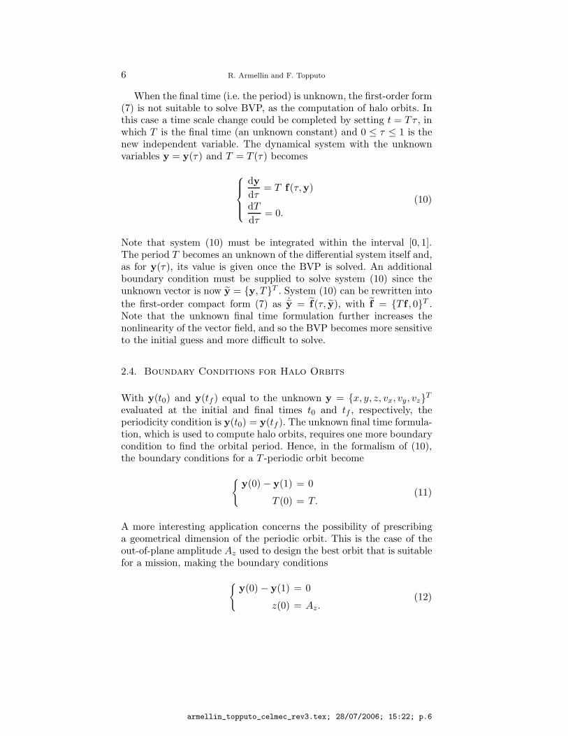
When the final time (i.e. the period) is unknown, the first-order form(7) is not suitable to solve BVP, as the computation of halo orbits. Inthis case a time scale change could be completed by setting t = Tτ , inwhich T is the final time (an unknown constant) and 0 ≤ τ ≤ 1 is thenew independent variable. The dynamical system with the unknownvariables y = y(τ) and T = T (τ) becomes
dy
dτ= T f(τ,y)
dT
dτ= 0.
(10)
Note that system (10) must be integrated within the interval [0, 1].The period T becomes an unknown of the differential system itself and,as for y(τ), its value is given once the BVP is solved. An additionalboundary condition must be supplied to solve system (10) since theunknown vector is now y = y, TT . System (10) can be rewritten into
the first-order compact form (7) as ˙y = f(τ, y), with f = T f , 0T .Note that the unknown final time formulation further increases thenonlinearity of the vector field, and so the BVP becomes more sensitiveto the initial guess and more difficult to solve.
2.4. Boundary Conditions for Halo Orbits
With y(t0) and y(tf ) equal to the unknown y = x, y, z, vx, vy, vzT
evaluated at the initial and final times t0 and tf , respectively, theperiodicity condition is y(t0) = y(tf ). The unknown final time formula-tion, which is used to compute halo orbits, requires one more boundarycondition to find the orbital period. Hence, in the formalism of (10),the boundary conditions for a T -periodic orbit become
y(0) − y(1) = 0
T (0) = T.(11)
A more interesting application concerns the possibility of prescribinga geometrical dimension of the periodic orbit. This is the case of theout-of-plane amplitude Az used to design the best orbit that is suitablefor a mission, making the boundary conditions
A Sixth-Order Accurate Scheme for Solving TPBVP in Astrodynamics 7
The boundary conditions for the computation of quasi-periodic haloorbits in the R4BP are
y(0) − y(1) = 0
θ(0) = θ0
z(0) = Az,
(13)
in which the initial phase of the Sun θ0 must be prescribed to let system(9) to be supplemented by eight boundary conditions.
2.5. Low Thrust Optimal Transfer to Halo Orbits
The controlled R3BP
x − 2y =∂Ω3
∂x+ u1, y + 2x =
∂Ω3
∂y+ u2, z =
∂Ω3
∂z+ u3, (14)
can be rewritten in the first order form as
y = f(y,u), (15)
in which u = u1, u2, u3T and y = x, y, z, vx, vy, vz
T are the controland state vectors, respectively. We aim at minimizing the objectivefunction
J =
∫ tf
t0L(y,u, t) dt =
1
2
∫ tf
t0uTu dt, (16)
with prescribed initial and final conditions y0 and yf on the states andwithin the time interval [tf , t0]. Introducing the Lagrange multipliersλi, i = 1, ..., 6, the Euler–Lagrange equations read
y =∂H
∂λ, λ = −
∂H
∂y, 0 =
∂H
∂u, (17)
in which H = λT f + L is the Hamiltonian of the optimal control
problem. System (17) represents a set of differential algebraic equa-tions (DAEs) to be solved by substitution exploiting the last equationwhich provides the values of the control functions in terms of Lagrangemultipliers
ui = −λ3+i, i = 1, 2, 3. (18)
Hence, system (17) must be solved together with the following twelveboundary conditions
y(t0) = y0
y(tf ) = yf .(19)
Solving system (17) with boundary conditions (19) means finding thefunctions y = y(t) and λ = λ(t) for t ∈ [t0, tf ]; then, with relation (18),
the set of optimal control functions u = u(t) is derived. This problemis difficult to solve due to the high nonlinearities of the dynamics of theLagrange multipliers. Their lack of physical meaning makes it difficultto find an appropriate initial guess close to the final solution.
3. Sixth-Order Linear Multi-Point Method
In this section we report the sixth-order LMPM for the solution of theBVPs stated above (Quartapelle and Scandroglio, 2003). We refer tothe generic n first-order equations
y = f(t,y), (20)
supplemented by the appropriate n boundary conditions that are as-sumed to be of the general nonlinear form
g(y(ta),y(tb)) = 0. (21)
The problem is to solve (20) and (21) within a finite time interval[ta, tb], over a uniform grid consisting of N points so that the step sizeof the discretization is
h = ∆t =tb − taN − 1
, (22)
with the grid points defined by ti = ta + (i − 1)h, for i = 1, . . . , N .The problem is now discretized by a strategy akin to that classically
adopted to solve initial value problems for ODEs, namely, the linear
multi-step method. Due to the non-initial-value character of the first-order system associated with a boundary value problem, only centraldifference approximations are applied. Constructed below is the sixth-order accurate method belonging to the class of schemes called linear
multi-point methods to be distinguished from those developed for thetime integration of initial value problems.
3.1. Construction of the Sixth-Order Accurate Scheme
The sixth-order linear multi-point method is obtained by approximat-ing the differential system (20) at midpoints ti+1/2, i = 2, . . . , N − 2,by means of a general computational molecule involving four pointsand of two special molecules involving five points at the both ends ofthe integration interval, as illustrated by the following scheme. In thefigure, the • denotes the grid point of the computational moleculesinvolved in the discretization while the ♦ indicates the location chosenfor the discrete approximation of the equations.
A Sixth-Order Accurate Scheme for Solving TPBVP in Astrodynamics 9
t1 t2 t3 t4 t5 . . . . . . tN−3 tN−2 tN−1 tN
• ♦ • • • •
• • ♦ • •
• • ♦ • •
• • ♦ • •
• • ♦ • •
• • ♦ • •
• • ♦ • •
• • ♦ • •
• • ♦ • •
• • • • ♦ •
For the first special molecule associated with the left extreme, the rela-tion expressing the linear approximation to a scalar equation dy/dt =f(t, y) based on five points is given by
α1y1 + α2y2 + α3y3 + α4y4 + α5y5
= h(β1f1 + β2f2 + β3f3 + β4f4 + β5f5),(23)
in which fi = f(ti, yi). Generally, for any internal molecule with mid-point ti+1/2, the linear discretization based on four points is
α1yi−1 + α2yi + α3yi+1 + α4yi+2
= h(β1fi−1 + β2fi + β3fi+1 + β4fi+2).(24)
A special molecule using five points analogous to that in (23) is usedat the right end of the interval, leading to a total of N − 1 discreteequations approximating the first-order dynamical system. The αi andβi coefficients are now determined by imposing cancellation conditionsthat enforce the exact respect of the fundamental theorem of calculus
at the level of the discrete equations, according to the method followedin Quartapelle and Scandroglio (2003). After some computations, thevalues of the coefficients of the linear approximation are, for the twospecial five-point molecules
For completeness, let us explicitly write the set of computationalmolecules which involve the first grid points. Replacing αi and αi
through (25) and (26), the left hand side of the discrete equationsbecomes the following scheme
−4960 y1
3860 y2
1160 y3 0 0
−1160 y1 −27
60 y22760 y3
1160 y4
−1160 y2 −27
60 y32760 y4
1160 y5
−1160 y3 −27
60 y42760 y5
. . .
−1160 y4 −27
60 y5. . .
−1160 y5
. . .
. . .
(29)
The summation of the coefficients in each column of this triangularmatrix corresponds to “integrate” the left hand side of the discreteequations and therefore verifies the fundamental theorem of calculus,∫ tbta
dydt dt = y(tb) − y(ta), because the sum of all elements in each col-
umn is zero except for the first column whose total is −y1 = −y(ta).Analogously, the right hand side of the discrete equation is
A Sixth-Order Accurate Scheme for Solving TPBVP in Astrodynamics 11
It is worth noting that the summation of the βi and βi in the scheme(30) leads to an approximation of the definite integral coincident withthe Gregory quadrature formula of precision O(h6). Gregory formulasprovide the natural numerical quadrature for a known discrete functionon a uniform grid. In those formulas, the weight is constant at internalpoints except for those near to the ends of the integration interval whereend corrections are applied (Fox, 1957).
After discretizing the problem over a uniform grid of N points,N − 1 discrete equations in the scalar case could be derived becausethey correspond to the number of integration subintervals. The N -thequation, which allows one to solve the algebraic problem, is obtainedthrough the (scalar) boundary condition.
One feature of the sixth-order LMPM is that it attains an accuracybeyond the first Dahlquist stability barrier (Lambert, 1991). Dahlquist’stheorem states that the order of accuracy q of a stable linear methodbased on p points (namely, p − 1 steps), in the language of linearmulti-step methods, satisfies
q ≤
p − 1 if the method is explicit,p if p is even,p + 1 if p is odd.
The present O(h6) Linear Multi-Point discretization is implicit and itsgeneral molecule has p = 4 points; therefore, from Dahlquist’s theo-rem the highest order of accuracy attainable by the new method isexpected to be q = p = 4 while the construction guarantees an order ofaccuracy of six. The point is that the theorem pertains to linear multi-step methods for IVPs while the proposed O(h6) accurate method isestablished to solve BVPs, although expressed as a first-order system.In fact, the LMPM is characterized by the presence of a (block) row,to enforce the two-point boundary conditions, which contains nonzeroelements either in both the first and last block or along the entire row.It is the occurrence of this special row that allows the method with onlyfour points to reach the sixth-order accuracy and therefore to overcomethe first Dahlquist stability barrier. Note that Quartapelle and Rebay(1990) introduced fourth-order and sixth-order LMPM based on com-putational molecules with four and six points, respectively. Thus, theaccuracy of the two old schemes was within Dahlquist’s barrier andrequired a greater computational effort. On the contrary, the presentmethod reaches an O(h6) accuracy involving just four points. As aresult, a better computational efficiency is gained since fewer functionevaluations are needed, and an increased sparsity of the discretizationmatrix is reached.
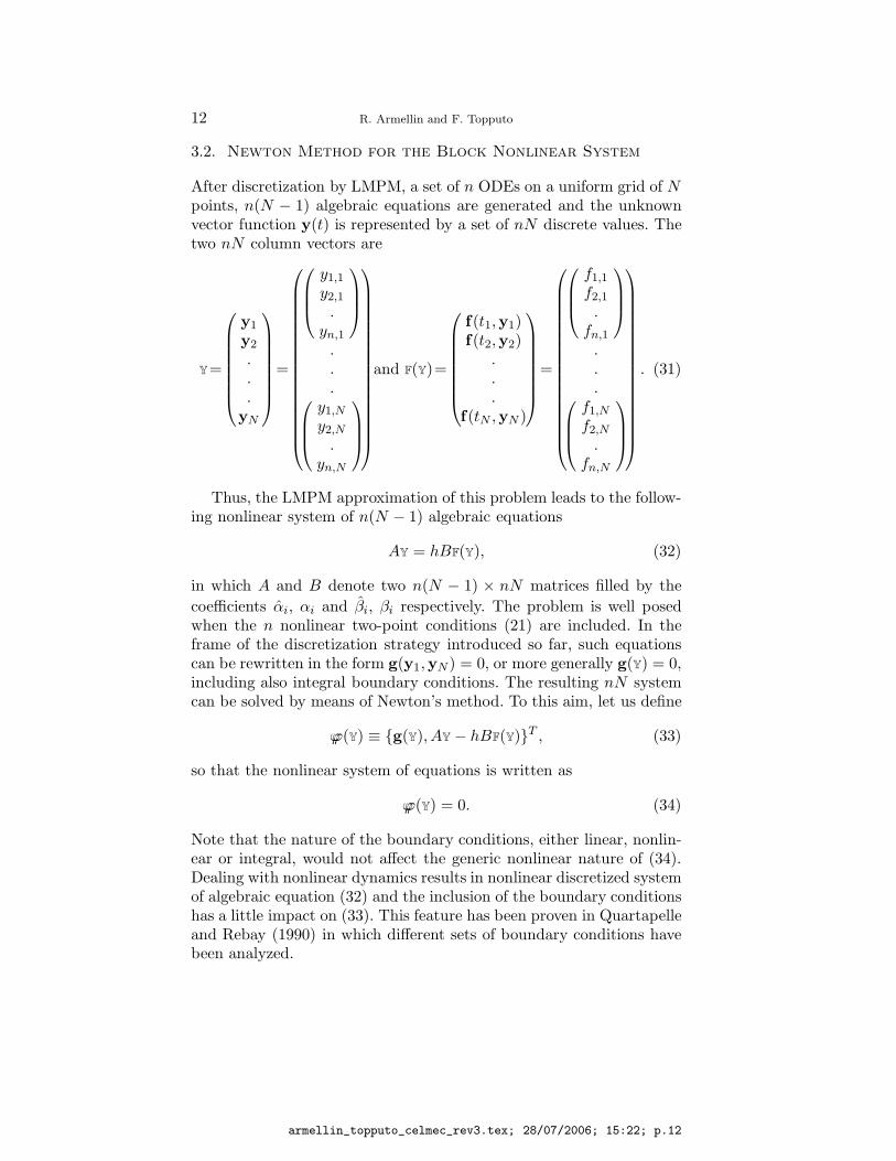
After discretization by LMPM, a set of n ODEs on a uniform grid of Npoints, n(N − 1) algebraic equations are generated and the unknownvector function y(t) is represented by a set of nN discrete values. Thetwo nN column vectors are
Y=
y1
y2
.
.
.yN
=
y1,1
y2,1
.yn,1
.
.
.
y1,N
y2,N
.yn,N
and F(Y)=
f(t1,y1)f(t2,y2)
.
.
.f(tN ,yN )
=
f1,1
f2,1
.fn,1
.
.
.
f1,N
f2,N
.fn,N
. (31)
Thus, the LMPM approximation of this problem leads to the follow-ing nonlinear system of n(N − 1) algebraic equations
AY = hBF(Y), (32)
in which A and B denote two n(N − 1) × nN matrices filled by the
coefficients αi, αi and βi, βi respectively. The problem is well posedwhen the n nonlinear two-point conditions (21) are included. In theframe of the discretization strategy introduced so far, such equationscan be rewritten in the form g(y1,yN ) = 0, or more generally g(Y) = 0,including also integral boundary conditions. The resulting nN systemcan be solved by means of Newton’s method. To this aim, let us define
ϕϕ(Y) ≡ g(Y), AY − hBF(Y)T , (33)
so that the nonlinear system of equations is written as
ϕϕ(Y) = 0. (34)
Note that the nature of the boundary conditions, either linear, nonlin-ear or integral, would not affect the generic nonlinear nature of (34).Dealing with nonlinear dynamics results in nonlinear discretized systemof algebraic equation (32) and the inclusion of the boundary conditionshas a little impact on (33). This feature has been proven in Quartapelleand Rebay (1990) in which different sets of boundary conditions havebeen analyzed.
A Sixth-Order Accurate Scheme for Solving TPBVP in Astrodynamics 13
Assuming an initial guess Y0 is given, its correction ∆Y0 defined byNewton’s method in incremental form is given by expanding ϕϕ(Y0 +∆Y0) around Y0 by the Taylor series to the second order
ϕϕ(Y0 + ∆Y0) ≈ ϕϕ(Y0) + J(Y0)∆Y0 = 0, (35)
in which
J(Y) ≡∂ϕϕ(Y)
∂Y=
∂g(Y)
∂Y
A − hB∂F(Y)
∂Y
. (36)
By solving equation (35) with respect to ∆Y0, we find
∆Y0 = −[J(Y0)]−1ϕϕ(Y0), (37)
and the new approximate solution Y1 is
Y1 = Y0 + γ∆Y0 = Y0 − γ[J(Y0)]−1ϕϕ(Y0). (38)
A full step of the Newton iteration is taken by setting γ = 1, otherwisea step size control can be introduced by taking 0 < γ < 1 allowing themethod to include a form of continuation to ease the convergence inthough problems. The linear system to be solved at the first iterationassumes the form
A 0∆Y0 = −ϕϕ(Y0), with A 0 =
∂g(Y)
∂Y
A − hB∂F(Y)
∂Y
Y=Y0
. (39)
Note that the nN -order Jacobian A 0 can be computed either ana-lytically evaluating the derivatives of both the vector field and theboundary condition, or numerically with a finite-difference approxima-tion. Thus, the UL factorization A 0 = U 0L 0 is used to determine thenew iterate by means of the substitutions
∆Y0 = −L−10 U
−10 ϕϕ(Y0). (40)
This is the solution to the linear system for the first step, while theincremental unknown ∆Yk for any subsequent iteration with k ≥ 0 isgiven by the relation
∆Yk = −L−1k U
−1k ϕϕ(Yk), (41)
in which U kL k = A k. Iterations terminate when the relative or theabsolute norm of the corrections is below the acceptable tolerance ε
‖∆Yk‖
‖Yk‖≤ ε if ‖Yk‖ ≥ 1 or ‖∆Yk‖ ≤ ε if ‖Yk‖ < 1. (42)
For completeness the algorithmic flow chart, the block bordered quadri-diagonal profile of the matrix A k, and the factorized triangular matrixesL k and U k are reported in appendixes A and B.
4. Astrodynamics Applications
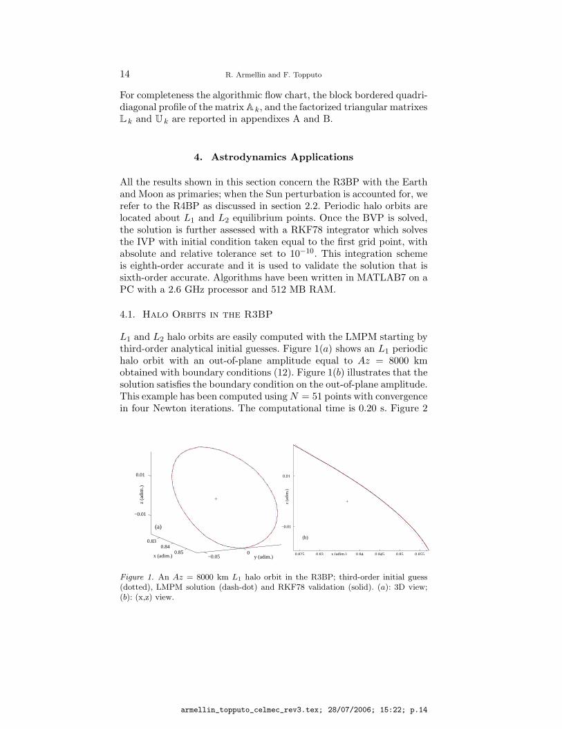
All the results shown in this section concern the R3BP with the Earthand Moon as primaries; when the Sun perturbation is accounted for, werefer to the R4BP as discussed in section 2.2. Periodic halo orbits arelocated about L1 and L2 equilibrium points. Once the BVP is solved,the solution is further assessed with a RKF78 integrator which solvesthe IVP with initial condition taken equal to the first grid point, withabsolute and relative tolerance set to 10−10. This integration schemeis eighth-order accurate and it is used to validate the solution that issixth-order accurate. Algorithms have been written in MATLAB7 on aPC with a 2.6 GHz processor and 512 MB RAM.
4.1. Halo Orbits in the R3BP
L1 and L2 halo orbits are easily computed with the LMPM starting bythird-order analytical initial guesses. Figure 1(a) shows an L1 periodichalo orbit with an out-of-plane amplitude equal to Az = 8000 kmobtained with boundary conditions (12). Figure 1(b) illustrates that thesolution satisfies the boundary condition on the out-of-plane amplitude.This example has been computed using N = 51 points with convergencein four Newton iterations. The computational time is 0.20 s. Figure 2
0.830.84
0.85−0.05
00.05
−0.01
0.01
y (adim.)x (adim.)
z (a
dim
.)
(a)
0.825 0.83 0.84 0.845 0.85 0.855
−0.01
0.01
x (adim.)
z (a
dim
.)
(b)
Figure 1. An Az = 8000 km L1 halo orbit in the R3BP; third-order initial guess(dotted), LMPM solution (dash-dot) and RKF78 validation (solid). (a): 3D view;(b): (x,z) view.
A Sixth-Order Accurate Scheme for Solving TPBVP in Astrodynamics 15
0.82 0.83 0.84 0.85 0.86 0.87−0.05
0
0.05−0.05
−0.04
−0.03
−0.02
−0.01
0
0.01
0.02
0.03
0.04
0.05
y (adim.)x (adim.)
z (a
dim
.)
(a)
1.121.14
1.161.18 −0.1
−0.050
0.050.1
−0.04
−0.02
0
0.02
0.04
y (adim.)x (adim.)
z (a
dim
.)
(b)
Figure 2. Families of halo orbits around L1 and L2. (a): L1 family; (b): L2 family.
illustrates the two families of halo orbits with amplitudes ranging from1000 to 20000 km. Using either boundary conditions (11) or (12), thesetwo families of orbits can be parameterized with T or Az as parameter.
4.2. Quasi-Periodic Halo Orbits in the R4BP
If LMPM is applied to compute halo orbits in the Sun-perturbed R4BPassuming the third-order initial guess and the eight boundary con-ditions (13), the algorithm does not converge. This problem can becircumvented by observing that if the mass of the Sun mS in equation(5) equals zero, the four-body dynamics degenerates into three-bodydynamics described by system of equations (1). This means that ifa halo orbit has been obtained in the R3BP, as the ones mentionedin the previous section, the parameter mS could be slightly increasedfrom zero to the final value mS = 3.2890 × 10⁵. Several intermediateBVPs, with vector field (9), boundary conditions (13), and an initialguess equal to the solution at the previous step, can be solved. In thiscase the LMPM is able to converge. This process is called numerical
continuation and the mass of the Sun is called continuation parameter.Note once again that, even if a set of solutions satisfying boundary
conditions (13) is found, they correspond to quasi-periodic orbits. Eventhough the values of position and the velocity coincide with those afterone revolution, the Sun moving in its circular orbit will cause the lossof this periodicity with successive revolutions.
4.2.1. Numerical Continuation of Quasi-Periodic Halos in the R4BP
The problem stated in section 2.4 for a definite value of mS is addressed.The nonlinear system of discrete equations for such a value is indicatedby
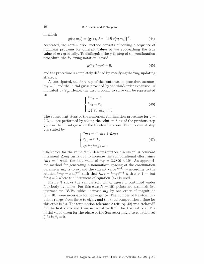
As stated, the continuation method consists of solving a sequence ofnonlinear problems for different values of mS approaching the truevalue of mS gradually. To distinguish the q-th step of the continuationprocedure, the following notation is used
ϕϕ(qY; qmS) = 0, (45)
and the procedure is completely defined by specifying the qmS updatingstrategy.
As anticipated, the first step of the continuation procedure assumesmS = 0, and the initial guess provided by the third-order expansion, isindicated by Yig. Hence, the first problem to solve can be representedas
1mS = 0
1Y0 = Yig
ϕϕ(1Y; 1mS) = 0.
(46)
The subsequent steps of the numerical continuation procedure for q =2, 3, . . . are performed by taking the solution q−1
Y of the previous stepq− 1 as the initial guess for the Newton iteration. The problem at stepq is stated by
qmS = q−1mS + ∆mS
qY0 = q−1
Y
ϕϕ(qY; qmS) = 0.
(47)
The choice for the value ∆mS deserves further discussion. A constantincrement ∆mS turns out to increase the computational effort since1mS = 0 while the final value of mS = 3.2890 × 10⁵. An appropri-ate method for generating a nonuniform spacing of the continuationparameter mS is to expand the current value q−1mS according to therelation qmS = c mq−1
S such that qmS = 1mScq−1 with c > 1 — butfor q = 2 where the increment of equation (47) is used.
Figure 3 shows the sample solution of figure 1 continued underfour-body dynamics. For this case N = 101 points are assumed; fiveintermediate BVPs, which increase mS by one order of magnitude(c = 10), were necessary for convergence. The number of Newton iter-ations ranges from three to eight, and the total computational time forthis orbit is 5 s. The termination tolerance ε (cfr. eq. 42) was “relaxed”for the first steps and then set equal to 10−10 for the last one. Theinitial value taken for the phase of the Sun accordingly to equation set(13) is θ0 = 0.
A Sixth-Order Accurate Scheme for Solving TPBVP in Astrodynamics 17
0.830.84
0.850.86−0.06−0.04−0.02 0 0.02 0.04 0.06
−0.02
0
0.02
y (adim.)x (adim.)
z (a
dim
.)
Figure 3. L1 halo orbit of figure 1 continued in the R4BP; orbit of figure 1 (dotted),LMPM solution (dash-dot) and RKF78 validation (solid).
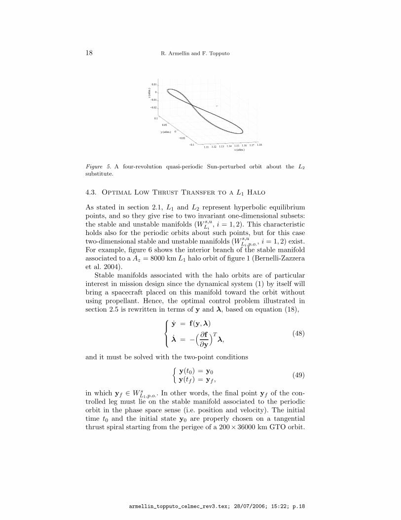
In analogy with the previous section, the whole L1 and L2 fami-lies of halo orbits, which are governed by four-body dynamics, havebeen computed. Each orbit is amplitude-parameterized by Az. Fur-thermore, supplying p-periodic initial guesses, it is possible to computequasi-periodic solutions orbiting p-times about the substitute of theequilibrium point. An example is illustrated in figure 5 in which anL2 quasi-periodic halo performs four revolutions. Nevertheless, suchkinds of solutions require an elevated computational effort because, asmentioned before, the Sun’s perturbations act to break the periodicityof the L2 halos. For example, the solution shown in figure 5 has beencomputed using N = 10000 (which means nN = 80000 variables in thiscase) points and its computation has been possible using the efficientfactorization algorithm reported in the appendix.
0.83 0.84 0.85 0.86 0.87 −0.050
0.05
−0.04
−0.02
0
0.02
0.04
0.06
y (adim.)x (adim.)
z (a
dim
.)
(a)
1.1 1.12 1.14 1.16 1.18−0.1 −0.05 0 0.05 0.1
−0.06
−0.04
−0.02
0
0.02
0.04
y (adim.)x (adim.)
z (a
dim
.)
(b)
Figure 4. Families of quasi-periodic halo orbits around the substitutes of L1 and L2
under the R4BP dynamics. (a): L1 family; (b): L2 family.
Figure 5. A four-revolution quasi-periodic Sun-perturbed orbit about the L2
substitute.
4.3. Optimal Low Thrust Transfer to a L1 Halo
As stated in section 2.1, L1 and L2 represent hyperbolic equilibriumpoints, and so they give rise to two invariant one-dimensional subsets:the stable and unstable manifolds (W s,u
Li, i = 1, 2). This characteristic
holds also for the periodic orbits about such points, but for this casetwo-dimensional stable and unstable manifolds (W s,u
Li,p.o., i = 1, 2) exist.For example, figure 6 shows the interior branch of the stable manifoldassociated to a Az = 8000 km L1 halo orbit of figure 1 (Bernelli-Zazzeraet al. 2004).
Stable manifolds associated with the halo orbits are of particularinterest in mission design since the dynamical system (1) by itself willbring a spacecraft placed on this manifold toward the orbit withoutusing propellant. Hence, the optimal control problem illustrated insection 2.5 is rewritten in terms of y and λ, based on equation (18),
y = f(y,λ)
λ = −( ∂f
∂y
)Tλ,
(48)
and it must be solved with the two-point conditions
y(t0) = y0
y(tf ) = yf ,(49)
in which yf ∈ W sL1,p.o.. In other words, the final point yf of the con-
trolled leg must lie on the stable manifold associated to the periodicorbit in the phase space sense (i.e. position and velocity). The initialtime t0 and the initial state y0 are properly chosen on a tangentialthrust spiral starting from the perigee of a 200× 36000 km GTO orbit.
A Sixth-Order Accurate Scheme for Solving TPBVP in Astrodynamics 19
−0.6 −0.4 −0.2 0 0.2 0.4 0.6 0.8 1
−0.8
−0.6
−0.4
−0.2
0
0.2
0.4
x (adim.)y
(adi
m.)
WsL1,p.o.
Earth Moon
Figure 6. Interior branch of the W sL1,p.o. (Bernelli-Zazzera et al. 2004).
The final time tf has been selected to be consistent with the choice ofinitial conditions.
Figure 7 shows an example of the solution to the optimal controlproblem stated above. After the tangential thrust leg, which determinesthe initial point y0, the BVP (48) and (49) is solved, and the rightboundary condition sets the point yf to lie on the stable manifoldbranch. The solution has been validated using a RKF78 integrationscheme and a cubic spline interpolation of the optimal control values.The algorithm has been able to converge using N = 1001 grid points.
The initial tangential thrust u = 2×10⁻⁴ m/s2 acts for a time equalto t0. Its value is an order of magnitude greater than the optimal controllaw, reported in figure 8(a), and contributes mostly to the computationof the propellant mass fraction necessary for the transfer, defined by
−0.8 −0.6 −0.4 −0.2 0 0.2 0.4 0.6 0.8 1−0.8
−0.6
−0.4
−0.2
0
0.2
0.4
0.6
0.8
yf
x (adim.)
y0
y (a
dim
.)
Tangential thrust spiral
W sL1,p.o.
Figure 7. An example of the solution to the optimal control problem; tangentialthrust spiral (solid), solution with the LMPM and RKF78 + cubic spline validation(bold); stable manifold leg and L1 periodic orbit (solid).
Table I. Solutions found for the low thrust optimalcontrol problem.
f (adim.) t0 (adim.) tf (adim.) TOF (days)
0.0498 20 21 188.5
0.0498 20 22 192.9
0.0618 25 28 219.0
0.0737 30 31 232.0
0.0855 35 36 253.7
the rocket equation as
f =mp
m0= 1 − e
−
∫ t00
‖u(t)‖dt
Ispg0 . (50)
To derive f , a specific impulse Isp = 3000 s is assumed. Table I summa-rizes a set of five solutions found in terms of time interval, propellantmass fraction, and total time of flight (TOF), which includes the tan-gential thrust spiral, the optimal leg, and the stable manifold branch.The first row corresponds to the solution of figure (7).
5. Final Remarks
A linear multi-point method has been applied for the solution of severalrepresentative boundary value problems in astrodynamics. This methodis based on the discretization of the problem on a uniform grid by means
Figure 8. Optimal thrust profile and low thrust transfer trajectory relative to thesolution of figure 7. (a): Optimal control law; (b): Trajectory in the Earth-centeredframe.
A Sixth-Order Accurate Scheme for Solving TPBVP in Astrodynamics 21
of a sixth-order accurate scheme. In practice, the proposed formulationexpresses the solution of the BVP in first-order form, and it becomesan ordinary matter of numerical nonlinear algebra. Simultaneously,the profile of the block matrices is bordered quadri-diagonal, and thisstructure can be easily preserved by properly choosing the direction inthe factorization and elimination process.
Such a solution scheme has been applied to generate halo orbits fromboth the restricted three- and four-body problems. While in the formercase the families of L1 and L2 halo orbits have been easily computed,the latter required a numerical continuation method for convergence.Thanks to numerical efficiency, each BVP has been solved in fractionsof a second. Furthermore, the LMPM has been applied to solve an openproblem in astrodynamics (Senent et al. 2005) concerning the designof trajectories reaching the halo orbits by combining low thrust andinvariant manifolds. The associated optimal control problem, stated bythe Euler–Lagrange system of equations, have been solved comfortably.
Finally, in figure 9 the error values versus grid-point number isshown. Since the analyzed problems do not have any analytical so-lutions, the error can be defined as e = |yN − yf |∞ where yf =ϕ(t0, tf ,y1) is the solution at time tf flowed with the RKF78 integrator(relative and absolute tolerance set to 10−12) starting from (t0,y1). Inthis context y1 and yN represent the unknowns corresponding respec-tively to first and to the final mesh point. The maximum distance, inthe phase space sense, between the solution given by LMPM and thevalidated orbit in figure 1 is e = 5.85 10−8 (N = 51), while the maxi-mum error of the solution in figure 3 is e = 3.07 10−7 (N = 101). Theoptimal control problem has been validated with the same integrationmethod which implements a cubic interpolation of the control force
102
103
10−12
10−10
10−8
10−6
10−4
10−2
100
N (grid points)
e (a
dim
.)
halo (R3BP)halo (R4BP)opt. contr. (R3BP)
Figure 9. The points (N , e) relative to the three astrodynamics application discussedin the previous sections.
history ui, i = 1, . . . , N . The solution in figure 7 (N=1001) has a finalerror equal to e = 4.41 10−9 which is much less than the thrust level.
We conclude by emphasizing once more the extreme efficiency, flex-ibility and reliability of the proposed method which is based on analgebraic transcription of the original differential problem.
Acknowledgements
The authors are strongly indebted to prof. Luigi Quartapelle for hispassionate collaboration and for sharing his effective software.
Appendix
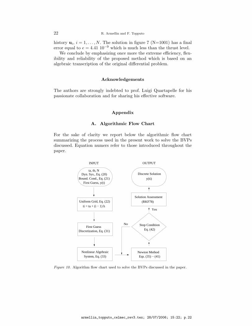
A. Algorithmic Flow Chart
For the sake of clarity we report below the algorithmic flow chartsummarizing the process used in the present work to solve the BVPsdiscussed. Equation numers refer to those introduced throughout thepaper.
ta, tb, NDyn. Sys., Eq. (20)
Bound. Cond., Eq. (21)First Guess, y(t)
Uniform Grid, Eq. (22)
ti = ta + (i − 1) h
First GuessDiscretization, Eq. (31)
Nonlinear AlgebraicSystem, Eq. (33)
Newton MethodEqs. (35) − (41)
Eq. (42)Stop Condition
Solution Assessment
(RKF78)
Discrete Solution
y(ti)
INPUT OUTPUT
No
Yes
Figure 10. Algorithm flow chart used to solve the BVPs discussed in the paper.
A Sixth-Order Accurate Scheme for Solving TPBVP in Astrodynamics 23
B. Factorization of the Bordered Quadri-Diagonal Matrix
The solution ∆Yk at the k iteration is given by ∆Yk = A−1k ϕϕ(Yk) and
is determined by a UL block factorization of the matrix of the system,Ak = UkLk. The adoption of the UL factorization proceeding from thebottom right corner in place of the more classical UL factorization isneeded to avoid the fill-in of the zero triangle comprised between thefirst row and the band of the matrix.
The matrix Ak of this system has the block bordered quadri-diagonalprofile, with four extra-band elements associated with the two specialcomputational molecules based on five points at the interval extremes.The profile of the block matrix associated with the O(h6) LMPM isgiven for completeness.
Ak =
G1 G2 G3 G4 G5 · · · GN−2 GN−1 GN
B1 C2 D3 D2 D1
A1 B2 C3 D4
A2 B3 C4 D5
A3 B4 C5 D6
· · · ·
· · · ·
· · · ·
AN−4 BN−3 CN−2 DN−1
BN AN−3 BN−2 CN−1 DN
AN AN−1 AN−2 BN−1 CN
Notice the four extra quadri-diagonal blocks for the first and lastspecial molecule, with five points stored as blocks D2, D1, AN andAN−1 to exploit the first two and last two available unused entries ofthe block diagonals Di and Ai, respectively. Notice furthermore thatin the matrix profile an additional block BN has been added to thesecond last row. This block is initially empty but must be retainedin the matrix profile since the block factorization process fills-in thisposition with nonzero values. We wish to emphasize that the first rowof Ak represents the discretized boundary conditions. This row is non-zero if integral boundary conditions are supplied; otherwise only G1
and GN are full.The factorization algorithm produces the block, bordered upper-bi-
diagonal matrix and block lower-tri-diagonal matrix below.
A Sixth-Order Accurate Scheme for Solving TPBVP in Astrodynamics 25
Simo, C., Gomez, G., Jorba, A. and Masdemont, J. (1995). “The Bicircular Modelnear the Triangular Libration Points of the RTBP”, in From Newton to Chaos,A.E. Roy & B.A. Steves (Eds.), Plenum Press, New York, pp. 343–370.
Bryson, A.E. and Ho, Y.C. (1975). Applied Optimal Control, John Wiley & Sons,New York.
Richardson, D.L. (1980) “Halo Orbit Formulation for the ISEE-3 Mission”. J. of
Guid. and Contr. 3, 543–548.Thurman, R. and Worfolk, P. (1996). The Geometry of Halo Orbits in the Circular
Restricted Three-Body Problem, Geometry Center Research Report, Universityof Minnesota, GCG95.
Masdemont, J.J. (2005) “High Order Expansions of Invariant Manifolds of LibrationPoint Orbits with Applications to Mission Design”. Dyn. Sys.: An Int. J., 20,59–113.
Gomez, G., Jorba, A., Masdemont, J. and Simo, C. (2000). Dynamics and Mission
Design near Libration Points – Volume III: Advanced Methods for Collinear
Points, World Scientific.Yagasaki, K. (2004) “Sun-Perturbated Earth-to-Moon Transfers with Low Energy
and Moderate Flight Time”. Cel. Mech. & Dyn. Astr., 90, 197–212.Fox, L. (1957). The Numerical Solution of Two-Point Boundary Value Problems in
Ordinary Differential Equations, Oxford University Press, Oxford.Lambert, J.D. (1991). Numerical Methods for Ordinary Differential Systems: The
Initial Value Problem, Wiley, Chichester.Bernelli-Zazzera, F., Topputo, F. and Massari, M. (2004). Assessment of Mission
Design Including Utilization of Libration Points and Weak Stability Boundaries,Final Report, ESTEC Contract No. 18147/04/NL/MV.
Senent, J., Ocampo, C. and Capella, A. (2005) “Low-Thrust Variable-Specific-Impulse Transfers and Guidance to Unstable Periodic Orbits”. J. of Guid.,


![Upwind schemes for the wave equation in second-order · PDF fileUpwind schemes for the wave equation in second-order form ... 3.5 A sixth-order accurate upwind scheme ... [5], the](https://static.documents.pub/doc/80x56/5a78efaf7f8b9a77088d5e04/upwind-schemes-for-the-wave-equation-in-second-order-schemes-for-the-wave-equation.jpg)


