2 School of Mechanical Engineering and Automation, Beihang University, Beijing 100191, China3 School of Transportation Science and Engineering, Beihang University, Beijing 100191, China4 School of Mechanical and Electrical Engineering, Lanzhou University of Technology, Lanzhou 730050, China;
Abstract: Electro-hydrostatic actuator (EHA) has significance in a variety of industrial tasks. Forthe purpose of elevating the working performance, we put forward a sliding mode control strategyfor EHA operation with a damping variable sliding surface. To start with, a novel sliding modecontroller and an extended state observer (ESO) are established to perform the proposed controlstrategy. Furthermore, based on the modeling of the EHA, simulations are carried out to analyze theworking properties of the controller. More importantly, experiments are conducted for performanceevaluation based on the simulation results. In comparison to the widely used control strategies, theexperimental results establish strong evidence of both overshoot suppression and system rapidity.
Electro-hydrostatic actuator (EHA) is considered a good solution in a wide rangeof industrial applications such as spacecraft [1], aircraft [2], robotics [3–6], vehicles [7],and heavy-duty suspension [8]. As a highly integrated power transmission system, EHAoutperforms traditional hydraulic systems by decreasing the weight and increasing theworking efficiency [9]. Typically, an electro-hydrostatic actuator (EHA) is a self-contained,pump-controlled system that is composed of a motor, a pump, a supercharged fuel tank,and a hydraulic cylinder (for simplification, the “hydraulic cylinder” is referred to as a“cylinder” in the rest of the paper) [10]. As such, by removing the hydraulic lines andservo valves, the system weight associated with the hydraulic tubing and the fluid iseliminated [11], while the system maintainability and reliability is improved [12]. Asreported in [13], “The last level of individualization is the separate assignment of the EHAsystems to each actuator. This configuration combines the best features of both hydraulicand electric technologies.”
Advances are ongoing to improve the working performance of hydraulic servo actua-tors. In the actuating domain, the nonlinearity and time variation of EHA have an impacton the dynamics as well as the servo control accuracy [14]. Research is still in progressto mitigate the deficiencies. Control strategy is one such field, with recent publicationshighlighting the significance of adaptive control (AC) [15], fuzzy control (FC) [16], feedbacklinearization control (FLC) [17], sliding mode control (SMC), and its improved extension,e.g., merging with proportion integration differentiation (PID) control [18,19], cascadecontrol (CC) [20], etc.
In an effort to address dynamic properties, current controlling applications mainlyfocus on exploring the potential of resolving the system uncertainties [21]. Encouragingly,
the sliding mode controller, due to its simple, robust, and accurate method of action, hasattracted a great deal of interest as one of the best controllers. The integration of relatedalgorithms, such the New Adaptive Reaching Law (NARL) [19] against chattering andthe extended state observer (ESO) [22] for working condition estimation, is verified. Stateobservers are commonly applied to control systems for the tasks of system uncertaintiesestimation and compensation [23–25]. In addition, Gao et al. constructed a two-stagesliding mode control to retain its rapidity and employed an improved Lyapunov functionto reduce system chattering [26]. Ren and Zhou presented a sliding mode controller witha fuzzy logic reasoning strategy, which provides faster adjustment time and higher accu-racy [27]. Notwithstanding, the problem of system overshoot caused by the large inertiaarises in heavy-duty operating applications where the stable actuating of EHA under loadhas important performance implications. Specifically, the contradiction between systemrapidity and overshooting, as the main concern, is most pronounced when establishing acontrol strategy [28]. Previous works used to take a smooth curve as an alternative of thestep signal in SMC [19,22]. In other words, an intact step input will cause the signal jumpin SMC, in which case a slow-settling output is formed to get a smaller overshoot [21].
For establishing an optimal control strategy for EHA operation, we propose a novelsliding mode control with damping variable sliding surface (DV-SMC) strategy. On theone hand, this control strategy aims at tackling the contradiction between settling time andthe overshoot with high robustness. On the other hand, the tuning of sliding mode surfaceparameters for DV-SMC is put forward. Together with the controller, an extended stateobserver is also designed to estimate and compensate for the control strategy. In line withEHA controlling, our controller, as a competitive alternative, can give rise to even betterworking performance. The contributions of this paper are as follows:
(1) To alleviate the conflict between the overshoot and rapidity of the EHA system, acontrol strategy based on SMC is proposed. Compared to the classical SMC method,the overshoot is suppressed without undermining the speed, which is in line withboth simulative and experimental results.
(2) For parameter adjustment, a parameter-tuning method for SMC is established. Forthe controller, damping-ratio-based parameter tuning is optimized, which furtherimproves the industrial applications of our controller.
Following the introduction, this research introduces background knowledge on EHAin Section 2, describes the proposed DV-SMC strategy in Section 3, shows the modeling andsimulating outcomes in Section 4, provides experimental results and analysis in Section 5,and finally presents conclusions and future research directions in Section 6.
2. Prerequisite
Figure 1 presents the working principle of the EHA. As mentioned above, the maincomponents of an EHA are a motor, a bidirectional pump, and an oil cylinder connected bymeter-in and meter-out valves. Specifically, a motor-driven pump without power trans-mission being hindered is employed; therefore, inefficient servo valves are eliminated [29].As a rule, the EHA performs flow rate control by a pump coupled to a motor. In Figure 1,the bold arrows indicate the flow of hydraulic oil. The control command, which drives themotor to rotate forward, is sent via the power drive electronics. Thus, oil is pumped intothe right chamber of the cylinder, which generates pressure and makes the cylinder moveto the left. Likewise, the reverse rotation of the motor leads to the left-to-right movementof the cylinder. That is, the load is driven by the moving of the cylinder for manipulatingan individual actuator. Accordingly, a closed control loop can be formed.
Actuators 2021, 10, 3 3 of 17Actuators 2021, 10, x FOR PEER REVIEW 3 of 19
Figure 1. Schematic diagram of an electro-hydrostatic actuator (EHA).
The modeling of the motor and the cylinder is presented as follows.
2.1. Brushless DC Motor (BLDCM) Model We employ a brushless DC motor (BLDCM), which is of high reliability, to drive the
pump in this research. Supposing the BLDCM is of Y-connection, the winding can be mathematically described as follows:
m e L m
e
J T T BU Li Ri K
ω ωω
= + − = + +
(1)
where U,L, i and R represent the equivalent voltage, inductance, current, and resistance; Ke is the back-electromotive force (EMF) coefficient; Te is the corresponding electromagnetic torque of the motor; Jm is the moment of inertia of the motor; Tl is the equivalent external load; and Bm is the viscous friction coefficient.
2.2. Pump-Controlled Cylinder Model Let Qi and Qo be the inlet and outlet flow of plunger pump. The working flow of the
EHA can be modeled as follows:
( ) ( )
( ) ( )
˙
˙
ini p i i o o i a i
e
outo p i i o o i a o
e
VQ D L p p L p p p
VQ D L p p L p p p
ωβ
ωβ
= − − − − − = − − − − −
(2)
where Dp is the pump displacement; Li and Lo represent the internal and external leakage coefficients; pi, po, and pa are the inlet pressure, outlet pressure, and back pressure of the oil tank pump; Vin and Vout are the equivalent inlet and outlet volume; and βe is the elastic modulus of the fluid.
Similarly, the dynamic model of the pump-controlled cylinder is denoted as follows:
( )
( )
in ll c l r
e
out rr c l r
e
V dpQ Ax L p p
dtV dpQ Ax L p p
dt
β
β
= + + − = − − −
(3)
where the subscripts l and r indicate the left- and right-hand sides of the cylinder chambers, respectively; A is the effective area of the piston rod; x is its displacement; and Lc stands for the internal leakage.
Due to the short flow passage inside the valve, the pressure loss within it is negligible. Notably, based on the flow continuity theorem, we have:
, , , l i r o l i r oQ Q Q Q p p p p= = = = . (4)
M
power driveelectronics
motorpump
regulating valve
cylinder
control command
load
m
Figure 1. Schematic diagram of an electro-hydrostatic actuator (EHA).
The modeling of the motor and the cylinder is presented as follows.
2.1. Brushless DC Motor (BLDCM) Model
We employ a brushless DC motor (BLDCM), which is of high reliability, to drive thepump in this research. Supposing the BLDCM is of Y-connection, the winding can bemathematically described as follows:
Jm.
ω = Te + TL − Bmω
U = L.i + Ri + Keω
(1)
where U,L,.i and R represent the equivalent voltage, inductance, current, and resistance; Ke
is the back-electromotive force (EMF) coefficient; Te is the corresponding electromagnetictorque of the motor; Jm is the moment of inertia of the motor; Tl is the equivalent externalload; and Bm is the viscous friction coefficient.
2.2. Pump-Controlled Cylinder Model
Let Qi and Qo be the inlet and outlet flow of plunger pump. The working flow of theEHA can be modeled as follows:
Qi = ωDp − Li(pi − po)− Lo(pi − pa)− Vinβe
.pi
Qo = ωDp − Li(pi − po)− Lo(pi − pa)− Voutβe
.po
(2)
where Dp is the pump displacement; Li and Lo represent the internal and external leakagecoefficients; pi, po, and pa are the inlet pressure, outlet pressure, and back pressure of the oiltank pump; Vin and Vout are the equivalent inlet and outlet volume; and βe is the elasticmodulus of the fluid.
Similarly, the dynamic model of the pump-controlled cylinder is denoted as follows:Ql = A
.x + Vin
βe
dpldt + Lc(pl − pr)
Qr = A.x− Vout
βe
dprdt − Lc(pl − pr)
(3)
where the subscripts l and r indicate the left- and right-hand sides of the cylinder chambers,respectively; A is the effective area of the piston rod; x is its displacement; and Lc stands forthe internal leakage.
Due to the short flow passage inside the valve, the pressure loss within it is negligible.Notably, based on the flow continuity theorem, we have:
Ql = Qi, Qr = Qo, pl = pi, pr = po. (4)
Actuators 2021, 10, 3 4 of 17
Thus, the model of the cylinder, by combining Equations (4) and (5), is definedas follows:
Dpω = A.x + V0
4βe∆
.p + La∆p + Qa
A∆p = M..x + Bc
.x + Ksx + Ff + FL
. (5)
In Equation (5), Vo represents the effective volume of the chamber; La is proportionalto the pressure difference ∆p is the total leakage coefficient of the pump and the cylinder;Qa is the unconsidered flow loss; M stands for the total equivalent mass of the cylinder andthe load; Bc is the viscous friction coefficient of the cylinder; Ks is the elastic load coefficient;Ff stands for the static friction; and FL is the load.
Based on Equations (1) and (5), X = [x1 x2 x3 x4 x5]T =
[x
.x ∆p ω ip
]T is establishedto characterize the system state, from which the EHA model can be written as follows:
.x1 = x2.x2 = A
M x3 − KsM x1 − Bc
M x2 −Ff +FL
M.x3 = 4βe
V0Dpx4 − 4Aβe
V0x2 − 4Lc βe
V0x3 + Qun
.x4 = 1
Ja
(Ktx5 − Bmx4 − Dpx3 − Tf
).x5 = 1
L (U − Rx5 − Kex4)
(6)
where Ja stands for the total rotational inertia of the motor and the pump.
2.3. Problem Formulation
According to Equation (6), x4 is a virtual control input with respect to the EHAmodel, based on which a three-order subsystem is formed by the first three equations.It can be observed that this high-order system contains both matched disturbances andmismatched disturbances. SMC is used to guarantee the robustness but is insensitive tomismatched disturbances [30,31]. Specifically, the control with mismatched disturbances ismore challenging than that with only matched disturbances, and only a few related resultshave been proposed [32].
In this way, we now redefine the state variables as Z = [z1 z2 z3 ]T =
[x1 x2
.x2]T .
Apparently, z1 z2 and z3 represent the position, velocity, and acceleration of the cylinder,respectively. Hence, the first three terms from Equation (6) can be elaborated on byEquation (7):
such that Qun stands for the flow loss that has not been considered.
3. Methodology
The proposed DV-SMC consists of two parts, i.e., a novel sliding mode controllerdesign and an extended state observer design. A stability analysis is presented as well.
Actuators 2021, 10, 3 5 of 17
3.1. Sliding Mode Controller with Damping Variable Sliding Surface
Originally, SMC was an approach for nonlinear controlling [33,34]. As pointed out inSection 1, the basic SMC shows great robustness against parameter uncertainties despiteits failure to deal with perturbations. Seeing as methods for attenuating the perturbationsare both productive and effective, we employed the exponential approach law to removethe perturbations and invoke the robustness of SMC [35,36].
On this occasion, a molded sliding mode controller is developed first. The systemerrors together with the derivatives are:
e = z1 − xd.e =
.z1 −
.xd..
e =..z1 −
..xd
(11)
Then, we choose the sliding surface σ as follows:
σ = c1.e + c2e +
..e (12)
where c1 and c2 are positive, which meets the requirements of the Routh-Hurwitz stabilitycriterion [37]. The error e, as such, approaches 0 during the control process.
Moreover, the exponential approach law is applied, which leads to:
.σ = c1
..e + c2
.e +
...e
= −εsign(σ). (13)
Furthermore, with u* representing the target value of the virtual control variable,we have
u∗ = g3−1(...x d − A3z3 − A2z2 − A1z1 + c1
..e + c2
.e)− εsign(σ). (14)
In Equations (12)–(14), the variation of c1 and c2 with respect to the controlling isrestricted to c1, c2 > 0. Despite the range of c1 and c2 within a two-dimensional plane, thevalues of these two parameters will inevitably affect the dynamic performance.
At this stage, we set the right side of Equation (12) to 0 to construct a transfer functionbetween x and xd, which is:
XXd
=s2 + c1s + c2
s2 + c1s + c2(15)
where s is the laplacian operator.A typical evaluation is to trace a step signal. In this case, as long as Xd is nonderivable
at the start time,.
Xd and..Xd do not exist in theory. However, in reality,
.Xd and
..Xd will
converge to the largest number instead of diverging to infinity. Furthermore, the enormousnumber can cause a saturation of control output (u* in Equation (14)) and a plunge ofoutput following the step moment, which results in an impact. However, this impact isthe source of a large overshoot or an oscillation during the system adjustment process. Forthis reason, the overshoot is limited by an artificial ceiling of
.Xd and
..Xd, as mentioned in
Section 1.Therefore, assuming that both
.xd and
..xd are 0 in the step response, the corresponding
transfer function is:XXd
=c2
s2 + c1s + c2. (16)
Notably, the transfer function in Equation (16) denotes a standard second-order oscilla-tion. Consequently, computation with c1 and c2 is facilitated by introducing the undampednatural frequency ωn and the damping ratio ξ, which are:
c1 = 2ξωn (17)
c2 = ωn2. (18)
Actuators 2021, 10, 3 6 of 17
One of the key facts is that the smaller ξ is, the faster the system response and thelarger the overshoot and oscillation that will be generated. Otherwise, the increase inξ can restrain the oscillation at the cost of settling time. Considering the contradictionbetween rapidity and stability, the damping ratio of 0.707 is a solution to a certain extent.In contrast, if the damping ratio is a changeable parameter, i.e., a small ξ for establishingsystem rapidity during the initial sliding and a large one for suppressing the overshoot inthe end, an even better response is possible.
Thus, we optimize the sliding surface presented in Equation (12):σn =
..e + γt
.e + ω2
neγt(e) = 2ωn(ξmin +
ξmax1+δe2 )
(19)
where ξmin and ξmax represent the minimum and maximum damping ratio and δ is thesensitivity factor for damping ratio regulating.
Thereafter, we can rewrite the transfer function from Equation (16) as follows:
XXd
=ωn
2
s2 + 2ωn
(ξmin +
ξmax1+δe2
)s + ωn2
. (20)
We have the system error e, starting with the sliding, as e 0, and ξmax(1 + δe2)−1 ≈ 0.
In this way, the damping ratio for the initial control phase is ξmin, which indicates an under-damped state with fast response. With the controlling system approaching its equilibrium,we have e→ 0 , while the damping ratio increases and finally reaches (ξmin + ξmax).
Accordingly, the adaptive regulation of ξ, within the interval (ξmin, ξmin + ξmax), cancater to the needs of system rapidity and stability via an optimal damping ratio. Thesensitivity factor δ is employed to determine the speed of the working damping ratioapproaching its upper and lower limits. When δ increases, ξ moves toward ξmin, andotherwise to (ξmin + ξmax) (see Figure 2).
Actuators 2021, 10, x FOR PEER REVIEW 7 of 19
Figure 2. Damping ratio changing along with error and sensitivity factor.
Then, in relation to the system parameter variation, we can compute the control out-put based on the virtual control variable. From Equation (14), we can compute the control law as follows:
( )( ) ( )
( )( )
* * 1 23 22
* 13 3 3 2 2 1 1
ˆ ˆ ˆˆ
ˆˆ
ˆˆ4
ˆ
ˆ1
ˆ
n maxd n t n
d d d
eeu u g e e e sign
e
u g x A z A z A z f t
ω ξ ω γ ε σδ
−
−
= + − + + + + = − − − −
(21)
3.2. Extended State Observer (ESO) State estimation requires knowledge of the plant, the control input, and the sensing
signals [38]. As presented in Equation (7), the EHA model is equivalent to a pure integral series system. Specifically, the parameter z1 is measured by a displacement sensor, from which z2 and z3 are derived by using a differentiator. The noise generated by the differen-tiator will cause the distortion of z2 and z3. Moreover, let ( )df t stand for the system dis-turbance, which is compensated for by the robust term in Equation (13). Nevertheless, this compensation is such an overcompensation that it can bring cause chattering in the steady phase of the servo system. For this reason, a fourth-order ESO, not only for estimating the system state, but also for revising the compensation via observing the system disturbance, is established in Equation (22):
( )( )
( )( )
2 1 1 1
22 3 2 1 1
33 3 3 1 1
4
1
4 4 1 1
ˆ ˆ ˆ
ˆ ˆˆ ˆ
ˆ
ˆ
ˆ
ˆp
z l z z
z z l z z
z g u h l z z
z l z
z
z
τ
τ
τ
τ
−
−
−
=
+ −
= + −
= + + −
= −
(22)
where 0 1τ< < , while [ ]1 2 3 4, , ,iL l l l l= is the gain matrix of ESO and is Hurwitz.
The total disturbance ˆph observed by ESO is:
( )3 3 2 2 1 1 ˆ ˆ ˆ ˆp dh A z A z A z f t= + + + (23)
The estimation error formula of ESO can be obtained with Equations (22) and (7), and is
Figure 2. Damping ratio changing along with error and sensitivity factor.
Then, in relation to the system parameter variation, we can compute the control outputbased on the virtual control variable. From Equation (14), we can compute the control lawas follows: u∗ = u∗d + g−1
3
[− 4ωn e
.eξmax
(1+δe2)2 + ωn
2.e + γt(e)
.e]+ εsign(σn)
u∗d = g−13
( ..xd − A3z3 − A2z2 − A1z1 − fd(t)
) (21)
3.2. Extended State Observer (ESO)
State estimation requires knowledge of the plant, the control input, and the sensingsignals [38]. As presented in Equation (7), the EHA model is equivalent to a pure integral
Actuators 2021, 10, 3 7 of 17
series system. Specifically, the parameter z1 is measured by a displacement sensor, fromwhich z2 and z3 are derived by using a differentiator. The noise generated by the differ-entiator will cause the distortion of z2 and z3. Moreover, let fd(t) stand for the systemdisturbance, which is compensated for by the robust term in Equation (13). Nevertheless,this compensation is such an overcompensation that it can bring cause chattering in thesteady phase of the servo system. For this reason, a fourth-order ESO, not only for esti-mating the system state, but also for revising the compensation via observing the systemdisturbance, is established in Equation (22):
Conforming to the convergence presented in Equation (30), the proposed observerhas the following characteristics: the state variable zi(i = 1, 2, 3) can converge toward itstrue value zi. Sequentially, G1 and E1 will finally approach 0, which is also the conditionfor |σn − σn|. As a result, when there is a sufficiently large ε, the result of
.Vn < 0 can be
obtained. Recall that ε in Equation (32) is not designed to fully compensate for the externaldisturbance fd(t). Notably, the ε here is far smaller than the ε in Equation (14). Similarly,the robust item in Equation (21) is far smaller than that in Equation (14). As expected, thesliding mode chattering can thereby be reduced.
The proof of control stability is complete. The DV-SM controller, together with the ESO,can respond to the demand of existence and reachability in line with the Lyapunov theory,which indicates that the proposed control strategy can be applied to the EHA operation.
4. Numerical Simulations4.1. Model Establishing
Numerical simulations are carried out to find suitable settings for the proposed DV-SMC strategy. In this research, a double-loop PID control scheme is taken as a representativeexample, which is implemented on the EHA together with the controller and its ESO.Specifically, a cascade control strategy is developed whereby the outer loop contains aDV-SM controller and the inner loop consists of a double-loop PID controller. The blockdiagram of the cascade controller is presented. As shown in Figure 3, the acquisition ofsensors is in real time, e.g., position x and current i. After the controller receives xd fromthe host computer, DV-SMC collects the state variables, i.e., zi (i = 1,2,3,4), from ESO togenerate the output u*. Consequently, the final output, which is exactly represented by uc
d,is calculated by dual-PID.
Actuators 2021, 10, x FOR PEER REVIEW 9 of 19
the external disturbance ( )df t . Notably, the ε here is far smaller than the ε in Equa-tion (14). Similarly, the robust item in Equation (21) is far smaller than that in Equation (14). As expected, the sliding mode chattering can thereby be reduced.
The proof of control stability is complete. The DV-SM controller, together with the ESO, can respond to the demand of existence and reachability in line with the Lyapunov theory, which indicates that the proposed control strategy can be applied to the EHA op-eration.
4. Numerical Simulations 4.1. Model Establishing
Numerical simulations are carried out to find suitable settings for the proposed DV-SMC strategy. In this research, a double-loop PID control scheme is taken as a representa-tive example, which is implemented on the EHA together with the controller and its ESO. Specifically, a cascade control strategy is developed whereby the outer loop contains a DV-SM controller and the inner loop consists of a double-loop PID controller. The block diagram of the cascade controller is presented. As shown in Figure 3, the acquisition of sensors is in real time, e.g., position x and current i. After the controller receives xd from the host computer, DV-SMC collects the state variables, i.e., zi (i = 1,2,3,4), from ESO to generate the output u*. Consequently, the final output, which is exactly represented by ucd, is calculated by dual-PID.
Figure 3. Block diagram of cascade control structure.
Bounded by the model of EHA in Equation (6), a second-order system with the input of voltage and output of motor spindle speed is constructed, as is the case for the double-loop PID controller. We have:
ds ps s is s ds sdc pc c ic c dc c
u K e K e dt K eu K e K e dt K e = + + = + +
(33)
where the subscripts s and c indicate the speed loop and the current loop, respectively; ( )* * ,du s c= stands for the control output of the current loop; and *e is the error of that
loop. For PID control, *pK , *iK , and *dK are the proportional coefficient, integral coef-ficient, and differential coefficient, respectively.
The configuration of the proposed EHA for simulation is given in Table 1.
m
PID
PIDESO
x
xdu*+ DV-SMC
ω
-
ucd
i
usd
-+
z1…z4
es
ec
Controllerhost
computer
Figure 3. Block diagram of cascade control structure.
Actuators 2021, 10, 3 9 of 17
Bounded by the model of EHA in Equation (6), a second-order system with the input ofvoltage and output of motor spindle speed is constructed, as is the case for the double-loopPID controller. We have:
uds = Kpses + Kis
∫esdt + Kds
.es
udc = Kpcec + Kic
∫ecdt + Kdc
.ec
(33)
where the subscripts s and c indicate the speed loop and the current loop, respectively;ud∗(∗ = s, c) stands for the control output of the current loop; and e∗ is the error of that loop.
For PID control, Kp∗, Ki∗, and Kd∗ are the proportional coefficient, integral coefficient, anddifferential coefficient, respectively.
The configuration of the proposed EHA for simulation is given in Table 1.
Table 1. Specifications for simulation initialization.
Parameter Value
Piston effective area(m2) 1.134× 10⁻³
Effective stroke (m) 0.1Leakage coefficient
(m3/(s/Pa)
)2.5× 10⁻¹¹
Fluid elastic modulus(N/m2) 6.86× 10⁸
Hydraulic cylinder volume(m3) 4× 10⁻⁴
Cylinder viscous friction (N/(m/s)) 1000Mass of cylinder and load (kg) 243Pump displacement
In order to verify the superiority of the DV-SMC strategy, an EHA system is built andoperated on MATLAB/Simulink software published by MathWorks. Inc. (Natick, MA,USA) with the same simulating input, different control strategies are conducted.
The control effect of three different strategies, i.e., three-loop PID control (labeled as“PID”), SMC with double-loop PID control (labeled “SMC”), and the proposed DV-SMCwith double-loop PID control (labeled “DV-SMC”), is compared to the reference input.Specifically, the inner loop of all three controllers is the same, which is double-loop PID.For the simulation, step signals of 50 mm, 15 mm, and 5 mm are sent to the system as areference for assessing the system tracking performance. As shown in Figure 4, the blacksolid line represents the reference control input, while the blue dotted line, red dotted line,and solid green line stand for the PID control, SMC, and DV-SMC, respectively.
In Figure 4, the conventional PID control fails to keep up with the various step signals.Through integration with the SMC and the DV-SMC, the tracking performance effect of thecontroller can be improved. The main reason for that is the system compensation as wellas the robustness against disturbance. On evaluating the settling time and the overshoot,we compare SMC and DV-SMC in line with the same input. Clearly, comparable resultsare obtained in terms of the settling time for both controllers. In contrast, the DV-SMcontroller is a better alternative for overshoot suppression. Giving an optimal dampingratio of 0.707, the maximum overshoot of the SM controller is 12%, 6.7%, and 6.7% for thethree reference inputs, respectively. On the other hand, there is no overshoot generatedwithin DV-SMC under each condition. Notably, the optimal damping ratio correspondsto SMC and still results in an over 5% overshoot during the sliding phase. A possibleexplanation is that the impact when approaching the sliding surface in the initial stage
Actuators 2021, 10, 3 10 of 17
will cause an overshoot in controlling. Since the proposed controller employs the adaptiveregulation of damping ratio, it is reasonable to expect a better overshoot suppression effect.The overdamping, based on the adaptive regulation of the damping ratio, can significantlyrestrain the overshoot when the error approaches 0 during the sliding process.
Actuators 2021, 10, x FOR PEER REVIEW 11 of 19
can significantly restrain the overshoot when the error approaches 0 during the sliding process.
(a) Response to 50 mm step input (b) Response to 15 mm step input
(c) Response to 5 mm step input
Figure 4. Simulation response to different reference inputs.
4.3. Damping Ratio Selection As pointed out in Section 3.1, the real damping ratio realξ of the controller ranges
from minξ to ( )min maxξ ξ+ . Corresponding simulations are carried out to figure out the values between minξ and ( )min maxξ ξ+ .
Let 0minξ = be the starting state to convey the deviation of e toward 0. Recall that the damping ratio close to 0 indicates a better working performance in the initial phase ac-cording to Equation (20). Thus, we have:
( )( ) 120 1 0real max eξ ξ δ−
= + + . (34)
Equation (33) means that the actual damping ratio is determined not only by the sen-sitivity factor δ but also by the maximum value of the deviation e. We set δ as a con-stant and 1δ = . Suppose we have ( )0e e= at the sliding surface, with ( )0e smaller than the effective stroke of EHA. During the sliding process, the value of realξ increases rapidly, conforming to the drop in e.
Likewise, maxξ identifies its significance in the response of the second half. The value of maxξ works on the effects of the system state approaching equilibrium point and the final suppression on overshoot. We set the values of maxξ to 0.5, 0.65, 0.8, 0.9, and 1. The step response of different maxξ is illustrated in Figure 5. The simulating outcomes show that the increasing damping ratio results in a decrease in the second-half overshoot and the adjustment time. We see that the settling time drops from 0.8 s to 0.3 s, with maxξ
Figure 4. Simulation response to different reference inputs.
4.3. Damping Ratio Selection
As pointed out in Section 3.1, the real damping ratio ξreal of the controller ranges fromξmin to (ξmin + ξmax). Corresponding simulations are carried out to figure out the valuesbetween ξmin and (ξmin + ξmax).
Let ξmin = 0 be the starting state to convey the deviation of e toward 0. Recall thatthe damping ratio close to 0 indicates a better working performance in the initial phaseaccording to Equation (20). Thus, we have:
ξreal = 0 + ξmax
(1 + δe(0)2
)−1. (34)
Equation (33) means that the actual damping ratio is determined not only by thesensitivity factor δ but also by the maximum value of the deviation e. We set δ as a constantand δ = 1. Suppose we have e = e(0) at the sliding surface, with e(0) smaller than theeffective stroke of EHA. During the sliding process, the value of ξreal increases rapidly,conforming to the drop in e.
Likewise, ξmax identifies its significance in the response of the second half. The valueof ξmax works on the effects of the system state approaching equilibrium point and thefinal suppression on overshoot. We set the values of ξmax to 0.5, 0.65, 0.8, 0.9, and 1. Thestep response of different ξmax is illustrated in Figure 5. The simulating outcomes showthat the increasing damping ratio results in a decrease in the second-half overshoot and
Actuators 2021, 10, 3 11 of 17
the adjustment time. We see that the settling time drops from 0.8 s to 0.3 s, with ξmaxincreasing from 0.5 to 1. Simultaneously, the overshoot is suppressed by about 20%. Basedon performance comparison, the configuration of ξmax within the interval [0.8,1] can beapplied for practical use. The ξmax of 0.8 can meet the demands of a steady responsewith a small amount of overshoot. For a system expecting a quick response without anyovershoot, the value of ξmax is set to 1.
Actuators 2021, 10, x FOR PEER REVIEW 12 of 19
increasing from 0.5 to 1. Simultaneously, the overshoot is suppressed by about 20%. Based on performance comparison, the configuration of maxξ within the interval [0.8,1] can be applied for practical use. The maxξ of 0.8 can meet the demands of a steady response with a small amount of overshoot. For a system expecting a quick response without any over-shoot, the value of maxξ is set to 1.
Figure 5. System response with different maxξ .
5. Experiments 5.1. Experimental Settings
Aiming to verify the working performance of the proposed control strategy, we con-duct the experiments with dedicatedly manufactured prototypes. Figure 6 shows the test rig. In this work, a prototype of the EHA is built for testing. The displacement of the actu-ator is detected by a position sensing element, while the sensing signals are transmitted to the controller via an encoder of SG37-2-09.52. Moreover, two pressure sensors are em-ployed for monitoring the pressure of the two piston cylinder chambers. The regulating valves are carried out for working mode switching, together with other experimental ap-paratus for facilitate the testing (Figure 6). More details of the EHA are given in Table 2.
Control commands, with 200 Hz sampling frequency, are originally performed on a host computer as the reference input conforming to the computational simulation. Power electronics are established for signal exchanging and processing. The control command is delivered from the host computer to the power electronics and then to the EHA as the system inputs. Specifically, the inputs of EHA consist of motor driving signals and valve signals. The former is generated by integrating the control commands and the system feedback, while the latter switches the operation mode. The system feedback, containing the motor current and the cylinder displacement, is sent back to the host computer via the power electronics. In this experiment, the feedback data are derived from a second-order Butterworth filter with a 40 Hz cutoff frequency, which is five times the referenced band-width of the EHA.
Figure 5. System response with different ξmax.
5. Experiments5.1. Experimental Settings
Aiming to verify the working performance of the proposed control strategy, weconduct the experiments with dedicatedly manufactured prototypes. Figure 6 shows thetest rig. In this work, a prototype of the EHA is built for testing. The displacement of theactuator is detected by a position sensing element, while the sensing signals are transmittedto the controller via an encoder of SG37-2-09.52. Moreover, two pressure sensors areemployed for monitoring the pressure of the two piston cylinder chambers. The regulatingvalves are carried out for working mode switching, together with other experimentalapparatus for facilitate the testing (Figure 6). More details of the EHA are given in Table 2.
Control commands, with 200 Hz sampling frequency, are originally performed on ahost computer as the reference input conforming to the computational simulation. Powerelectronics are established for signal exchanging and processing. The control commandis delivered from the host computer to the power electronics and then to the EHA as thesystem inputs. Specifically, the inputs of EHA consist of motor driving signals and valvesignals. The former is generated by integrating the control commands and the systemfeedback, while the latter switches the operation mode. The system feedback, containingthe motor current and the cylinder displacement, is sent back to the host computer viathe power electronics. In this experiment, the feedback data are derived from a second-order Butterworth filter with a 40 Hz cutoff frequency, which is five times the referencedbandwidth of the EHA.
Actuators 2021, 10, 3 12 of 17Actuators 2021, 10, x FOR PEER REVIEW 13 of 19
Figure 6. Schematic of test rig.
Table 2. Specifications of EHA.
Parameter Value Rated pressure ( )MPa 11 Rated speed ( )mm / s 300
Rated force ( )kN 12 Effective displacement ( )mm 0 ~ 110 Rated power supply ( )VDC 270
Bandwidth ( )Hz 5
5.2. Results A 5000 N external load is applied to the cylinder of the EHA beforehand. Based on
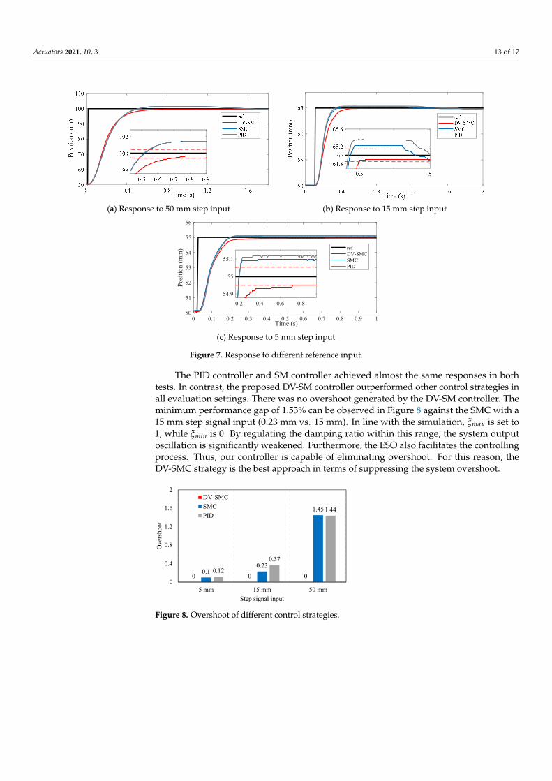
the simulating results, we refer to the control inputs as 5 mm, 15 mm, and 50 mm step signals and apply the reference inputs to the three controllers, i.e., the PID controller, the SM controller, and the DV-SM controller mentioned in Section 4.2. Figure 7 shows the results of the controlling tasks carried out using all reference inputs. In these figures, all the controllers obtain a trend consistent with the simulation outcomes. To further validate the working properties, the overshoot and settling time of different controllers are presented in Figures 8 and 9.
Figure 6. Schematic of test rig.
Table 2. Specifications of EHA.
Parameter Value
Rated pressure (MPa) 11Rated speed (mm/s) 300
Rated force (kN) 12Effective displacement (mm) 0 ∼ 110Rated power supply (VDC) 270
Bandwidth (Hz) 5
5.2. Results
A 5000 N external load is applied to the cylinder of the EHA beforehand. Based onthe simulating results, we refer to the control inputs as 5 mm, 15 mm, and 50 mm stepsignals and apply the reference inputs to the three controllers, i.e., the PID controller, theSM controller, and the DV-SM controller mentioned in Section 4.2. Figure 7 shows theresults of the controlling tasks carried out using all reference inputs. In these figures, all thecontrollers obtain a trend consistent with the simulation outcomes. To further validate theworking properties, the overshoot and settling time of different controllers are presented inFigures 8 and 9.
Actuators 2021, 10, 3 13 of 17Actuators 2021, 10, x FOR PEER REVIEW 14 of 19
(a) Response to 50 mm step input (b) Response to 15 mm step input
(c) Response to 5 mm step input
Figure 7. Response to different reference input.
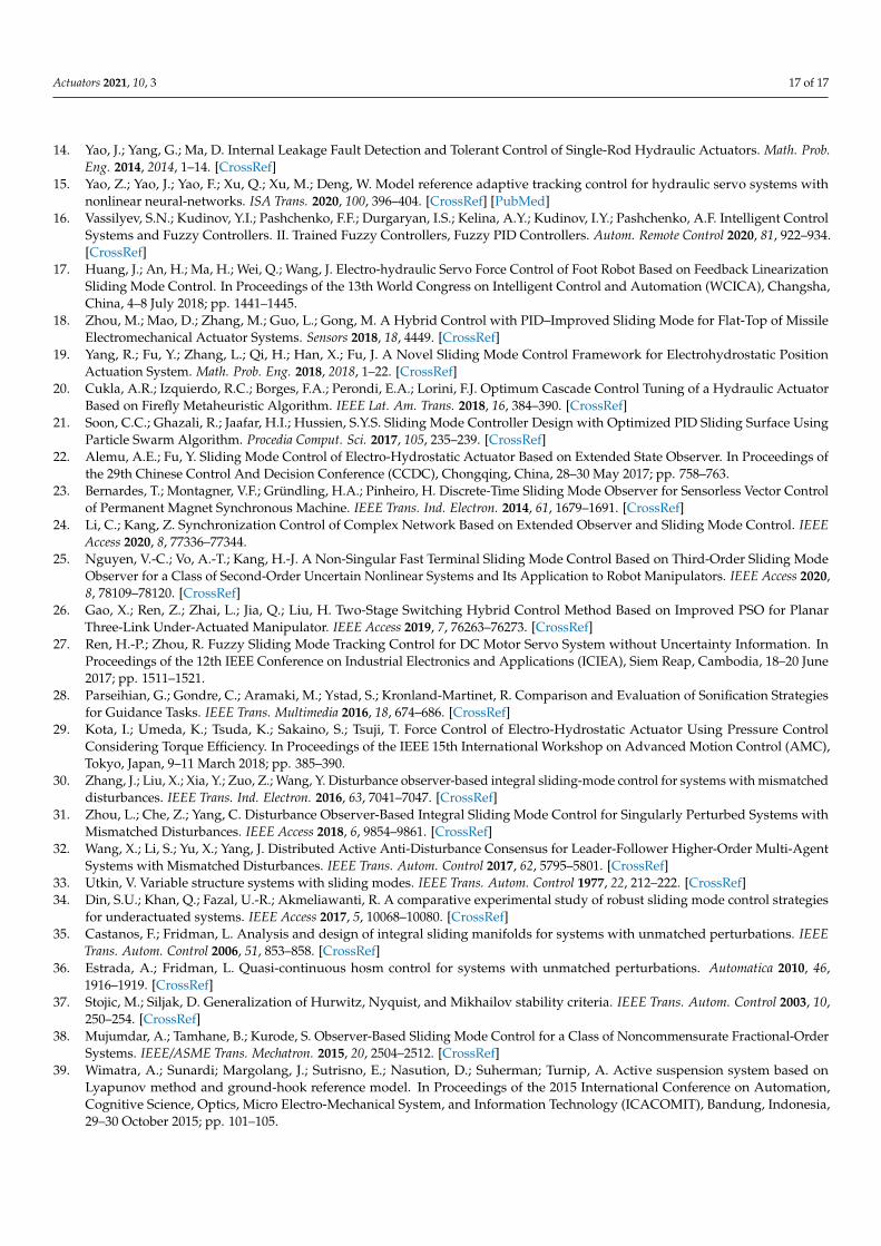
The PID controller and SM controller achieved almost the same responses in both tests. In contrast, the proposed DV-SM controller outperformed other control strategies in all evaluation settings. There was no overshoot generated by the DV-SM controller. The minimum performance gap of 1.53% can be observed in Figure 8 against the SMC with a 15 mm step signal input (0.23 mm vs. 15 mm). In line with the simulation, maxξ is set to 1, while minξ is 0. By regulating the damping ratio within this range, the system output oscillation is significantly weakened. Furthermore, the ESO also facilitates the controlling process. Thus, our controller is capable of eliminating overshoot. For this reason, the DV-SMC strategy is the best approach in terms of suppressing the system overshoot.
Figure 8. Overshoot of different control strategies.
0 0.1 0.2 0.3 0.4 0.5 0.6 0.7 0.8 0.9 1Time (s)
50
51
52
53
54
55
56
Position (mm) ref
DV-SMCSMCPID
0.2 0.4 0.6 0.854.9
55
55.1
0 0 00.1
0.23
1.45
0.12
0.37
1.44
0
0.4
0.8
1.2
1.6
2
5 mm 15 mm 50 mm
Overshoot
Step signal input
DV-SMCSMCPID
Figure 7. Response to different reference input.
The PID controller and SM controller achieved almost the same responses in bothtests. In contrast, the proposed DV-SM controller outperformed other control strategies inall evaluation settings. There was no overshoot generated by the DV-SM controller. Theminimum performance gap of 1.53% can be observed in Figure 8 against the SMC with a15 mm step signal input (0.23 mm vs. 15 mm). In line with the simulation, ξmax is set to1, while ξmin is 0. By regulating the damping ratio within this range, the system outputoscillation is significantly weakened. Furthermore, the ESO also facilitates the controllingprocess. Thus, our controller is capable of eliminating overshoot. For this reason, theDV-SMC strategy is the best approach in terms of suppressing the system overshoot.
Actuators 2021, 10, x FOR PEER REVIEW 14 of 19
(a) Response to 50 mm step input (b) Response to 15 mm step input
(c) Response to 5 mm step input
Figure 7. Response to different reference input.
The PID controller and SM controller achieved almost the same responses in both tests. In contrast, the proposed DV-SM controller outperformed other control strategies in all evaluation settings. There was no overshoot generated by the DV-SM controller. The minimum performance gap of 1.53% can be observed in Figure 8 against the SMC with a 15 mm step signal input (0.23 mm vs. 15 mm). In line with the simulation, maxξ is set to 1, while minξ is 0. By regulating the damping ratio within this range, the system output oscillation is significantly weakened. Furthermore, the ESO also facilitates the controlling process. Thus, our controller is capable of eliminating overshoot. For this reason, the DV-SMC strategy is the best approach in terms of suppressing the system overshoot.
Figure 8. Overshoot of different control strategies.
0 0.1 0.2 0.3 0.4 0.5 0.6 0.7 0.8 0.9 1Time (s)
50
51
52
53
54
55
56
Position (mm) ref
DV-SMCSMCPID
0.2 0.4 0.6 0.854.9
55
55.1
0 0 00.1
0.23
1.45
0.12
0.37
1.44
0
0.4
0.8
1.2
1.6
2
5 mm 15 mm 50 mm
Overshoot
Step signal input
DV-SMCSMCPID
Figure 8. Overshoot of different control strategies.
Actuators 2021, 10, 3 14 of 17Actuators 2021, 10, x FOR PEER REVIEW 15 of 19
Figure 9. Settling time of different control strategies. 1+ in Figure 9 represents that the settling time of SMC and PID on the 5 mm step input is longer than the signal collecting time (1s).
Consistent results are obtained for the settling time comparison. For system rapidity description, we define a settling time as the first time to stabilize within the range of 1%±reference input. In Figure 9, one can see that the proposed DV-SMC is still the best-performing resolution among the three controllers. The explanation for this issue is quite similar to that of the simulation results. The overshoot occurs because of saturated output of SMC and PID as well as the inertia of the workload. In contrast, the DV-SMC strategy maintains its output when it first reaches the controlling accuracy range. As shown in Figure 9, in terms of settling time, the proposed DV-SMC still exceeds the performance of the other methods.
Regarding the controlling outputs, results show the stability of the three controllers; see Figure 10. Generally, DV-SMC withdraws the output saturation and reaches the stabilization within a short time. Corresponding to the system response, our method is superior in overshoot suppression and reverse output preclusion. During the steady-state phase, the sign function pre-proposed in (26) is replaced by a saturation function ( )sat * in Equation (34). It is worth noticing that the system oscillation is significantly restrained, with the control output fluctuating slightly.
( )( )
( )( )
1, if * 1sat * *, if 1 * 1
1, if * 1
≥= − < < − ≤
(35)
Additionally, Figure 11 shows the outcomes of the sinusoidal tracking test. The SM controller, due to its nonlinear robust compensation, is able to overcome the impact of the dead zone without topping phenomenon. At the point of x 0= , the output rise on the SM controller can result in a more stable state of EHA. By contrast, there is a dead-time effect on the PID control output. In spite of the feedforward compensation of dX and dX , the DV-SM controller exploits the compensation effect of ESO. According to Figure 11, com-pared to the SM controller, our model obtains a better tracking result. The maximum ab-solute errors (MAE), as well as the mean square errors (MSE) of the models, are presented in Figure 12, which confirms the stability of our controller in sinusoidal tracking tasks. The effectiveness of the variable damping strategy, in terms of suppressing overshoot, leads us to conclude that DV-SMC has a more stable step response.
0.72
0.5
0.71
1+1.16
1.46
1+
1.415 1.45
0
0.4
0.8
1.2
1.6
5 mm 15 mm 50 mm
Settling tim
e/s
Step signal input
DV-SMCSMCPID
Figure 9. Settling time of different control strategies. 1+ in Figure 9 represents that the settling timeof SMC and PID on the 5 mm step input is longer than the signal collecting time (1s).
Consistent results are obtained for the settling time comparison. For system rapiditydescription, we define a settling time as the first time to stabilize within the range of±1% reference input. In Figure 9, one can see that the proposed DV-SMC is still the best-performing resolution among the three controllers. The explanation for this issue is quitesimilar to that of the simulation results. The overshoot occurs because of saturated outputof SMC and PID as well as the inertia of the workload. In contrast, the DV-SMC strategymaintains its output when it first reaches the controlling accuracy range. As shown inFigure 9, in terms of settling time, the proposed DV-SMC still exceeds the performance ofthe other methods.
Regarding the controlling outputs, results show the stability of the three controllers;see Figure 10. Generally, DV-SMC withdraws the output saturation and reaches thestabilization within a short time. Corresponding to the system response, our method issuperior in overshoot suppression and reverse output preclusion. During the steady-statephase, the sign function pre-proposed in (26) is replaced by a saturation function sat(∗)in Equation (34). It is worth noticing that the system oscillation is significantly restrained,with the control output fluctuating slightly.
sat(∗) =
1, if(∗ ≥ 1)
∗, if(−1 < ∗ < 1)−1, if(∗ ≤ 1)
(35)
Additionally, Figure 11 shows the outcomes of the sinusoidal tracking test. The SMcontroller, due to its nonlinear robust compensation, is able to overcome the impact of thedead zone without topping phenomenon. At the point of
.x = 0, the output rise on the SM
controller can result in a more stable state of EHA. By contrast, there is a dead-time effect onthe PID control output. In spite of the feedforward compensation of
.Xd and
..Xd, the DV-SM
controller exploits the compensation effect of ESO. According to Figure 11, compared tothe SM controller, our model obtains a better tracking result. The maximum absolute errors(MAE), as well as the mean square errors (MSE) of the models, are presented in Figure 12,which confirms the stability of our controller in sinusoidal tracking tasks. The effectivenessof the variable damping strategy, in terms of suppressing overshoot, leads us to concludethat DV-SMC has a more stable step response.
Actuators 2021, 10, 3 15 of 17Actuators 2021, 10, x FOR PEER REVIEW 16 of 19
(a) Control output of 50 mm step input (b) Control output of 15 mm step input
(c) Control output of 5mm step input
Figure 10. Control output of different reference inputs.
(a) Sinusoidal tracking outcomes (b) Control output of sinusoidal input
Figure 11. Sinusoidal tracking outcomes.
.
Figure 12. Tracking error of different controllers.
Control output
0 1 2 3 4 5Time (s)
−150
−100
−50
0
50
100
150
200DV-SMCSMCPID
1.7 1.75 1.8 1.85
0
40
80
Figure 10. Control output of different reference inputs.
Actuators 2021, 10, x FOR PEER REVIEW 16 of 19
(a) Control output of 50 mm step input (b) Control output of 15 mm step input
(c) Control output of 5mm step input
Figure 10. Control output of different reference inputs.
(a) Sinusoidal tracking outcomes (b) Control output of sinusoidal input
Figure 11. Sinusoidal tracking outcomes.
.
Figure 12. Tracking error of different controllers.
Control output
0 1 2 3 4 5Time (s)
−150
−100
−50
0
50
100
150
200DV-SMCSMCPID
1.7 1.75 1.8 1.85
0
40
80
Figure 11. Sinusoidal tracking outcomes.
Actuators 2021, 10, x FOR PEER REVIEW 16 of 19
(a) Control output of 50 mm step input (b) Control output of 15 mm step input
(c) Control output of 5mm step input
Figure 10. Control output of different reference inputs.
(a) Sinusoidal tracking outcomes (b) Control output of sinusoidal input
Figure 11. Sinusoidal tracking outcomes.
.
Figure 12. Tracking error of different controllers.
Control output
0 1 2 3 4 5Time (s)
−150
−100
−50
0
50
100
150
200DV-SMCSMCPID
1.7 1.75 1.8 1.85
0
40
80
Figure 12. Tracking error of different controllers.
6. Conclusions
In this research, a novel sliding mode control strategy with a damping variable slidingsurface, composed of a damping variable sliding mode controller and an extended state
Actuators 2021, 10, 3 16 of 17
observer, was designed and deployed for EHA controlling. Computational modeling andsimulations were established to preliminarily analyze the properties of the DV-SMC. Inline with the simulation, experimental results revealed that the proposed DV-SMC withdouble-loop PID control outperformed the other control strategies in the evaluation of bothovershoot suppression and settling time. As a result, we came to the following conclusions.
Firstly, in EHA operations, the frequency and damping ratio from the second-orderoscillation are assessed on the sliding mode surface of SMC. The parameters of the DV-SMCfor EHA controlling were defined, which also paved the way for parameter tuning of SMC.
Secondly, the control strategy simulation verified the system response in comparisonto a three-loop PID controller and SMC with double-loop PID controller. Simulationoutcomes indicated the effectiveness of the variable damping sliding mode surface inrestraining overshoot and oscillation. Moreover, the optimal value range of the dampingratio was determined.
Lastly, we performed an experiment showing the capability of the proposed DV-SMC with double-loop PID control via an EHA working system. Even better workingperformance in overshoot suppression and settling time was achieved. Our controller canbe an optimal approach for catering to the demands of EHA controlling.
Author Contributions: Conceptualization, M.W., Y.F. and D.Z.; methodology, M.W., Y.W. and R.Y.;software, M.W.; validation, Y.W.; formal analysis, Y.F.; investigation, R.Y.; resources, D.Z.; datacuration, Y.F. and D.Z.; writing—original draft preparation, M.W.; writing—review and editing, M.W.,Y.W., R.Y., Y.F. and D.Z.; visualization, M.W. and R.Y.; supervision, Y.F., D.Z.; project administration,Y.F. All authors have read and agreed to the published version of the manuscript.
Funding: This research is a general project supported by the National Natural Science Foundation ofChina (No. 61520106010) and the Chinese Civil Aircraft Project (MJ-2017-S49).
Acknowledgments: The authors acknowledge the English review process conducted by MDPI services.
Conflicts of Interest: The authors declare no conflict of interest.
References1. Sarigiannidis, A.G.; Beniakar, M.E.; Kakosimos, P.E.; Kladas, A.G.; Papini, L.; Gerada, C. Fault tolerant design of fractional slot
winding permanent magnet aerospace actuator. IEEE Trans. Transport. Electrific. 2016, 2, 380–390. [CrossRef]2. Qiao, G.; Liu, G.; Shi, Z.; Wang, Y.; Ma, S.; Lim, T.C. A review of electromechanical actuators for More/All Electric aircraft systems.
J. Mech. Eng. Sci. 2018, 232, 4128–4151. [CrossRef]3. Staman, K.; Veale, A.J.; Kooij, H. The PREHydrA: A Passive Return, High Force Density, Electro-Hydrostatic Actuator Concept
for Wearable Robotics. IEEE Rob. Autom. Lett. 2018, 3, 3569–3574. [CrossRef]4. Lee, T.; Lee, D.; Song, B.; Baek, Y.S. Design and Control of a Polycentric Knee ExoskeletonUsing an Electro-Hydraulic Actuator.
Sensors 2020, 20, 211. [CrossRef] [PubMed]5. Lee, D.; Song, B.; Park, S.Y.; Baek, Y.S. Development and Control of an Electro-Hydraulic Actuator System for an Exoskeleton
Robot. Appl. Sci. 2019, 9, 4295. [CrossRef]6. Nguyen, H.T.; Trinh, V.C.; Le, T.D. An Adaptive Fast Terminal Sliding Mode Controller of Exercise-Assisted Robotic Arm for
Elbow Joint Rehabilitation Featuring Pneumatic Artificial Muscle Actuator. Acutators 2020, 9, 118. [CrossRef]7. Miller, T.B. Preliminary Investigation on Battery Sizing Investigation for Thrust Vector Control on Ares I and Ares V Launch
Vehicles. February 2011. Available online: https://ntrs.nasa.gov/api/citations/20110007153/downloads/20110007153 (accessedon 22 December 2020).
8. Sun, W.; Gao, H.; Yao, B. Adaptive Robust Vibration Control of Full-Car Active Suspensions With Electrohydraulic Actuators.IEEE Trans. Control Syst. Technol. 2013, 21, 2417–2422. [CrossRef]
9. Shang, Y.; Li, X.; Qian, H.; Wu, S.; Pan, Q.; Huang, L.; Jiao, Z. A Novel Electro Hydrostatic Actuator System with Energy RecoveryModule for More Electric Aircraft. IEEE Trans. Ind. Electron. 2020, 67, 2991–2999. [CrossRef]
10. Ren, G.; Esfandiari, M.; Song, J.; Sepehri, N. Position Control of an Electrohydrostatic Actuator with Tolerance to Internal Leakage.IEEE Trans. Control Syst. Technol. 2016, 24, 2224–2232. [CrossRef]
11. Maré, J.-C.; Fu, J. Review on signal-by-wire and power-by-wire actuation for more electric aircraft. Chin. J. Aeronaut. 2017, 30,857–870. [CrossRef]
12. Guo, Q.; Zhang, Y.; Celler, B.G.; Su, S.W. State-constrained control of single-rod electrohydraulic actuator with parametricuncertainty and load disturbance. IEEE Trans. Control Syst. Technol. 2018, 26, 2242–2249. [CrossRef]
13. Lee, W.; Li, S.; Han, D.; Sarlioglu, B.; Minav, T.A.; Pietola, M. A Review of Integrated Motor Drive and Wide-Bandgap PowerElectronics for High-Performance Electro-Hydrostatic Actuators. IEEE Trans. Transp. Electrification. 2018, 4, 684–693. [CrossRef]
14. Yao, J.; Yang, G.; Ma, D. Internal Leakage Fault Detection and Tolerant Control of Single-Rod Hydraulic Actuators. Math. Prob.Eng. 2014, 2014, 1–14. [CrossRef]
15. Yao, Z.; Yao, J.; Yao, F.; Xu, Q.; Xu, M.; Deng, W. Model reference adaptive tracking control for hydraulic servo systems withnonlinear neural-networks. ISA Trans. 2020, 100, 396–404. [CrossRef] [PubMed]
17. Huang, J.; An, H.; Ma, H.; Wei, Q.; Wang, J. Electro-hydraulic Servo Force Control of Foot Robot Based on Feedback LinearizationSliding Mode Control. In Proceedings of the 13th World Congress on Intelligent Control and Automation (WCICA), Changsha,China, 4–8 July 2018; pp. 1441–1445.
18. Zhou, M.; Mao, D.; Zhang, M.; Guo, L.; Gong, M. A Hybrid Control with PID–Improved Sliding Mode for Flat-Top of MissileElectromechanical Actuator Systems. Sensors 2018, 18, 4449. [CrossRef]
19. Yang, R.; Fu, Y.; Zhang, L.; Qi, H.; Han, X.; Fu, J. A Novel Sliding Mode Control Framework for Electrohydrostatic PositionActuation System. Math. Prob. Eng. 2018, 2018, 1–22. [CrossRef]
20. Cukla, A.R.; Izquierdo, R.C.; Borges, F.A.; Perondi, E.A.; Lorini, F.J. Optimum Cascade Control Tuning of a Hydraulic ActuatorBased on Firefly Metaheuristic Algorithm. IEEE Lat. Am. Trans. 2018, 16, 384–390. [CrossRef]
22. Alemu, A.E.; Fu, Y. Sliding Mode Control of Electro-Hydrostatic Actuator Based on Extended State Observer. In Proceedings ofthe 29th Chinese Control And Decision Conference (CCDC), Chongqing, China, 28–30 May 2017; pp. 758–763.
24. Li, C.; Kang, Z. Synchronization Control of Complex Network Based on Extended Observer and Sliding Mode Control. IEEEAccess 2020, 8, 77336–77344.
25. Nguyen, V.-C.; Vo, A.-T.; Kang, H.-J. A Non-Singular Fast Terminal Sliding Mode Control Based on Third-Order Sliding ModeObserver for a Class of Second-Order Uncertain Nonlinear Systems and Its Application to Robot Manipulators. IEEE Access 2020,8, 78109–78120. [CrossRef]
26. Gao, X.; Ren, Z.; Zhai, L.; Jia, Q.; Liu, H. Two-Stage Switching Hybrid Control Method Based on Improved PSO for PlanarThree-Link Under-Actuated Manipulator. IEEE Access 2019, 7, 76263–76273. [CrossRef]
27. Ren, H.-P.; Zhou, R. Fuzzy Sliding Mode Tracking Control for DC Motor Servo System without Uncertainty Information. InProceedings of the 12th IEEE Conference on Industrial Electronics and Applications (ICIEA), Siem Reap, Cambodia, 18–20 June2017; pp. 1511–1521.
28. Parseihian, G.; Gondre, C.; Aramaki, M.; Ystad, S.; Kronland-Martinet, R. Comparison and Evaluation of Sonification Strategiesfor Guidance Tasks. IEEE Trans. Multimedia 2016, 18, 674–686. [CrossRef]
29. Kota, I.; Umeda, K.; Tsuda, K.; Sakaino, S.; Tsuji, T. Force Control of Electro-Hydrostatic Actuator Using Pressure ControlConsidering Torque Efficiency. In Proceedings of the IEEE 15th International Workshop on Advanced Motion Control (AMC),Tokyo, Japan, 9–11 March 2018; pp. 385–390.
30. Zhang, J.; Liu, X.; Xia, Y.; Zuo, Z.; Wang, Y. Disturbance observer-based integral sliding-mode control for systems with mismatcheddisturbances. IEEE Trans. Ind. Electron. 2016, 63, 7041–7047. [CrossRef]
31. Zhou, L.; Che, Z.; Yang, C. Disturbance Observer-Based Integral Sliding Mode Control for Singularly Perturbed Systems withMismatched Disturbances. IEEE Access 2018, 6, 9854–9861. [CrossRef]
32. Wang, X.; Li, S.; Yu, X.; Yang, J. Distributed Active Anti-Disturbance Consensus for Leader-Follower Higher-Order Multi-AgentSystems with Mismatched Disturbances. IEEE Trans. Autom. Control 2017, 62, 5795–5801. [CrossRef]
33. Utkin, V. Variable structure systems with sliding modes. IEEE Trans. Autom. Control 1977, 22, 212–222. [CrossRef]34. Din, S.U.; Khan, Q.; Fazal, U.-R.; Akmeliawanti, R. A comparative experimental study of robust sliding mode control strategies
for underactuated systems. IEEE Access 2017, 5, 10068–10080. [CrossRef]35. Castanos, F.; Fridman, L. Analysis and design of integral sliding manifolds for systems with unmatched perturbations. IEEE
Trans. Autom. Control 2006, 51, 853–858. [CrossRef]36. Estrada, A.; Fridman, L. Quasi-continuous hosm control for systems with unmatched perturbations. Automatica 2010, 46,
1916–1919. [CrossRef]37. Stojic, M.; Siljak, D. Generalization of Hurwitz, Nyquist, and Mikhailov stability criteria. IEEE Trans. Autom. Control 2003, 10,
250–254. [CrossRef]38. Mujumdar, A.; Tamhane, B.; Kurode, S. Observer-Based Sliding Mode Control for a Class of Noncommensurate Fractional-Order
Systems. IEEE/ASME Trans. Mechatron. 2015, 20, 2504–2512. [CrossRef]39. Wimatra, A.; Sunardi; Margolang, J.; Sutrisno, E.; Nasution, D.; Suherman; Turnip, A. Active suspension system based on
Lyapunov method and ground-hook reference model. In Proceedings of the 2015 International Conference on Automation,Cognitive Science, Optics, Micro Electro-Mechanical System, and Information Technology (ICACOMIT), Bandung, Indonesia,29–30 October 2015; pp. 101–105.