A small estimated euro area model with rational expectations and

WORKING PAPER NO. 30

A SMALL ESTIMATEDEURO AREA MODEL WITH

RATIONAL EXPECTATIONSAND NOMINAL RIGIDITIES

BY GÜNTER COENENAND VOLKER WIELAND

September 2000

E U R O P E A N C E N T R A L B A N K

WORKING PAPER SERIES

WORKING PAPER NO. 30

A SMALL ESTIMATEDEURO AREA MODEL WITH

RATIONAL EXPECTATIONSAND NOMINAL RIGIDITIES*,**

BY GÜNTER COENENAND VOLKER WIELAND

September 2000

E U R O P E A N C E N T R A L B A N K

WORKING PAPER SERIES

* Correspondence: Coenen: Directorate General Research, European Central Bank, Frankfurt am Main, Germany, tel.: (0)69 1344-7887, e-mail: [email protected]; Wieland: Federal ReserveBoard, Washington, DC, 20009, U.S.A., tel.: (202) 736-5620, e-mail: [email protected], Homepage: http://www.volkerwieland.com.

** The opinions expressed are those of the authors and do not necessarily reflect views of the European Central Bank or the Board of Governors of the Federal Reserve System. Volker Wieland servedas a consultant at the European Central Bank while preparing this paper. We are grateful for research assistance by Anna-Maria Agresti from the European Central Bank. And we greatly appreciatehelpful comments by Volker Clausen, Jeffrey Fuhrer, Thomas Laubach, Andrew Levin, Athanasios Orphanides, Richard Porter, John Taylor and by seminar participants at the European Central Bank, theKiel Institute of World Economics, the KU Leuven, the Deutsche Bundesbank and the CEF 2000 conference in Barcelona, where the first version of the paper from February 2000 was presented. Anyremaining errors are of course the sole responsibility of the authors.

© European Central Bank, 2000

Address Kaiserstrasse 29

D-60311 Frankfurt am Main

Germany

Postal address Postfach 16 03 19

D-60066 Frankfurt am Main

Germany

Telephone +49 69 1344 0

Internet http://www.ecb.int

Fax +49 69 1344 6000

Telex 411 144 ecb d

All rights reserved.

Reproduction for educational and non-commercial purposes is permitted provided that the source is acknowledged.

The views expressed in this paper are those of the authors and do not necessarily reflect those of the European Central Bank.

ISSN 1561-0810

ECB Working Paper No 30 ��September 2000 3

Contents

Abstract 5

1 Introduction 7

2 Modelling inflation dynamics with overlapping contracts 11

3 The data 16

4 Empirical inflation and output dynamics 19

5 Estimating the overlapping contracts specifications 225.1 The reduced-form representation 225.2 Estimates of the structural parameters 245.3 Further sensitivity analysis 29

6 Closing the model: Output gaps and interest rates 32

7 Evaluating monetary policy rules: An example 35

8 Summary and concluding remarks 38

References 40

Annexes 44

European Central Bank Working Paper Series 67

ECB Working Paper No 30 ��September 20004


Abstract

The objective of this paper is to estimate a small model of the euro area to be used as a laboratoryfor evaluating the performance of alternative monetary policy strategies. We start with therelationship between output and inflation and investigate the fit of the nominal wage contractingmodel due to Taylor (1980) and three different versions of the relative real wage contracting modelproposed by Buiter and Jewitt (1981) and estimated by Fuhrer and Moore (1995a) for the UnitedStates. While Fuhrer and Moore reject the nominal contracting model and find strong evidence infavor of the relative contracting model which induces a higher degree of inflation persistence, wefind that both types of contracting models fit euro area data reasonably well. The best fittingspecification is a version of the relative contracting model, but one that is theoretically moreplausible than the one preferred by Fuhrer and Moore for U.S. data.

A drawback of the euro area estimation is that the data are averaged over the member economies,which experienced different monetary policy regimes prior to the formation of EMU. WhereasGermany enjoyed stable inflation with fairly predictable monetary policy, countries such as Italy andFrance experienced a long-drawn out and probably imperfectly anticipated disinflation. Toinvestigate the validity of our results, we also obtain estimates for France, Germany and Italyseparately. We find that the relative contracting model does quite well in countries whichtransitioned out of a high inflation regime such as France and Italy, while the nominal contractingmodel fits German data better. Thus, an optimist may conclude that the independent EuropeanCentral Bank will face a similar environment in the future as the Bundesbank did in Germany andpick the nominal contracting specification, while a pessimist, who suspects that stabilizing euro areainflation will require higher output losses, may want to pick the relative contracting specification.We close the model by estimating an aggregate demand relationship and investigate theconsequences of the different wage contracting specifications for the output costs associated withstabilizing inflation, when interest rates are set according to Taylor�s rule.

JEL classification system: E31, E52, E58, E61Keywords: European Monetary Union, euro area, macroeconomic modelling, rational expectations, nominalrigidities, overlapping wage contracts, inflation persistence, monetary policy rules


1 Introduction

With the formation of European Monetary Union (EMU) in 1999, the eleven countries

that adopted the euro began to conduct a single monetary policy oriented towards union-

wide objectives.1 As prescribed by the Maastricht Treaty the primary goal of this policy

is to maintain price stability within the euro area. The operational definition of this goal

announced by the European Central Bank (ECB) is to aim for year-on-year increases in the

euro area inflation rate below 2 percent.2 To evaluate alternative strategies for achieving

such a euro-area-wide objective, it is essential to build empirical models that can be used to

assess the area-wide impact of policy on key macroeconomic variables such as output and

inflation. Thus, the objective of this paper is to construct a small model of the euro area,

which may serve as a laboratory for evaluating the performance of alternative monetary

policy strategies in the vein of recent studies for the United States.3

One possible approach to building a model of the euro area is to start by constructing

separate models of the individual member economies and then link them together in a multi-

country model. The main alternative is to first aggregate the relevant macroeconomic time

series across member economies, and then estimate a model for the euro area as a whole.

In this paper, we pursue the latter approach, the reason being that the objectives as well

as the instruments of Eurosystem monetary policy are defined on the euro area level. Of

course, a problem with this approach is that the data used in aggregation stem from periods1Austria, Belgium, Finland, France, Germany, Ireland, Italy, Luxembourg, the Netherlands, Portugal

and Spain. Denmark, Sweden, Greece and the U.K. have not adopted the euro. Their central banks are alsomembers of the European System of Central Banks, but not of the Eurosystem.

2As measured by the Harmonized Index of Consumer Prices (HICP). It was further clarified that thisdefinition excludes decreases and thus deflation. A detailed discussion of these and other issues regardingthe ECB’s strategy can be found in Angeloni, Gaspar and Tristani (1999).

3The recent literature on policy rules for the U.S. economy has used a variety of models: (i) small-scalebackward-looking models such as Rudebusch and Svensson (1999); (ii) large-scale backward-looking modelssuch as Fair and Howrey (1996); (iii) small-scale models with rational expectations and nominal rigidities(cf. Fuhrer and Moore (1995a), (1995b), Fuhrer (1997), Orphanides, Small, Wieland and Wilcox (1997), andOrphanides and Wieland (1998)); (iv) large-scale models of this type such as Taylor (1993a) and the FederalReserve Board’s FRB/US model (cf. Brayton et al. (1997), Reifschneider et al. 1999 ); and (v) small modelswith optimizing agents such as Rotemberg and Woodford (1997, 1999), Clarida, Galı and Gertler (1999,2000) and McCallum and Nelson (1999). Recent comparative studies of interest include Bryant, Hooper andMann (1993) and Taylor (1999a).

ECB Working Paper No 30 l September 2000 7

prior to EMU, when the different member economies experienced different monetary regimes

and policies. Therefore, we also estimate every model specification separately for the three

largest member economies, France, Germany and Italy, which together comprise over 70%

of economic activity in the euro area. By comparing the estimates obtained with French,

German and Italian data to the euro area estimates, we can assess to what extent the choice

of model specification for the euro area is influenced by the aggregation itself. Furthermore,

by comparing France and Italy, which experienced a convergence process prior to EMU,

with Germany, which enjoyed stable inflation and interest rates, we can see whether the

choice of specification is influenced by differences in the monetary regime prior to EMU.

In building our small-scale euro area model we start with the relationship between

inflation and output. In this respect we make two modelling assumptions, which are central

to the key policy tradeoff between inflation and output variability. We assume that market

participants form expectations in a forward-looking, rational manner and that monetary

policy has short-run real effects due to the existence of overlapping wage contracts. In the

long run, however, monetary policy is neutral. The assumption of rational expectations

constitutes a useful benchmark for policy evaluation, because the alternative assumption of

backward-looking expectations would imply that the central bank can exploit systematic

expectational errors by market participants.4

As to overlapping wage contracts, we explore the empirical fit of the nominal wage

contracting model due to Taylor (1980) as well as three different versions of the relative

real wage contracting model first proposed by Buiter and Jewitt (1981) and investigated

empirically by Fuhrer and Moore (1995a) for the United States. The nominal contracting

model belongs to the class of New-Keynesian sticky-price models which are consistent with

intertemporal optimization by imperfectly competitive firms.5 However, Fuhrer and Moore

(1995a) have argued that the nominal contracting model cannot explain the degree of in-4Thus, our analysis accounts for the Lucas critique in the narrow sense that market expectations take

into account the decision rule of the policymaker. However, it violates the Lucas critique in the widersense, because it does not explicitly take into account the optimizing behavior of individual and possiblyheterogeneous market participants.

5See Goodfriend and King (1997) for a comprehensive survey.

8 ECB Working Paper No 30 l September 2000

flation persistence observed in U.S. data, while the relative real wage contracting model

instead induces sufficient inflation stickiness. This difference has important policy implica-

tions, in particular regarding the costs of stabilizing inflation in terms of increased output

variability.

Comparing these alternative specifications, we find that the relative real wage contract-

ing model fits euro area inflation dynamics better than the nominal contracting model.

However, we also note that the nominal contracting model is not rejected by the data.

Among the three different versions of the relative real wage contracting model, it is not the

simplified specification preferred by Fuhrer and Moore, but a theoretically more plausible

specification, which obtains the best fit. Comparing the estimates for the individual coun-

tries, we find that the same relative wage contracting model fits Italian and French data

quite well, but not the German data, which exhibits a substantially lower degree of infla-

tion persistence. Only the nominal contracting model seems to have a shot at explaining

inflation dynamics in Germany.

Fuhrer and Moore’s empirical findings with U.S. data have generated a continuing debate

on the sources of inflation stickiness. For example, Roberts (1997) showed that a sticky-

inflation model with rational expectations is observationally equivalent to a sticky-price

model with expectations that are imperfectly rational. Using data on survey expectations

in the U.S., Roberts found evidence of backward-looking behavior. More recently, Sbordone

(1998) and Galı and Gertler (1999) have argued that the New-Keynesian sticky-price model

is capable of explaining U.S. inflation dynamics, if one uses a measure of marginal costs

rather than the output gap as the determinant of inflation.6 Finally, Taylor (1999b) has

pointed out that the level of inflation influences the pricing power of firms, and argued that

inflation is more persistent in a high inflation regime than in a low inflation regime with

credible monetary policy.

Our comparative analysis with European data contributes some new results to this de-6As the authors show, a model with price-stickiness is sufficient in this case, because marginal costs

themselves exhibit persistence. An open question, which needs to be settled in order to construct a completemacro model, concerns the source of the observed persistence in marginal costs.


bate. By assuming rational expecations, our estimation approach attributes the large degree

of inflation persistence in France and Italy and the euro area as a whole to structural nom-

inal rigidities. An alternative interpretation of this finding is to consider it evidence of

adaptive expectations as suggested by Roberts (1997) in the context of the U.S. inflation

process. This interpretation is also a plausible explanation of the observed degree of per-

sistence, because the convergence process experienced by those countries may at best have

been imperfectly anticipated by market participants. Thus, as far as the future of the EMU

is concerned, the estimation based on historical euro area data might overstate the case

for the relative real wage contracting model. Further support for this interpretation of our

results is provided by the better fit of the nominal contracting model in Germany, where

inflation was rather stable and monetary policy fairly predictable. The estimation results

with German data also provide indirect empirical support for the thesis that the degree of

inflation persistence is lower in a stable monetary policy regime with low average inflation,

because of the change in the pricing power of firms as suggested by Taylor (1999b).

In estimating euro area, French and Italian inflation dynamics with pre-EMU data,

we use the deviations of inflation from the downward trend rather than the inflation rate

itself. This downward trend was generated by the convergence of inflation in Italy, France,

Spain and other EMU member countries to German levels from the late 1970s until the

late 1990s. Our estimates for Germany, however, are based on actual inflation rates since

Germany experienced rather stable inflation. The downward trend is a unique feature of

historical euro area data and should not be expected to persist nor to be reversed in the

future, if the ECB achieves its policy objective. The short-run variations around this trend,

however, to the extent that they were due to structural rigidities, may still help predicting

the inflation dynamics after the formation of EMU. We discuss the use of inflation deviations

from trend in more detail when we describe the data and investigate its implications for the

estimation results later on.

In terms of evaluating alternative monetary policy strategies for the euro area, an analyst

who is pessimistic about the output losses associated with stabilizing inflation might prefer


to use the relative contracting model, while an optimist might prefer the nominal contracting

model. A robust monetary policy strategy, however, should perform reasonably well under

both specifications. We provide an illustrative example for the case of Taylor’s rule.

The remainder of the paper proceeds as follows. Section 2 reviews the overlapping

contracts specifications. The data is discussed in section 3. Section 4 summarizes inflation

and output dynamics in form of unconstrained VAR models, while the structural estimates

obtained by means of simulation-based indirect inference methods are reported in section

5. In section 6 we close the model with an aggregate demand equation, a term structure

relationship and a policy rule. Impulse responses and disinflation scenarios under alternative

specifications are compared in section 7. Section 8 concludes and the appendix provides the

details of the indirect estimation methodology.

2 Modelling inflation dynamics with overlapping contracts

We estimate four different specifications of overlapping wage contracts, the nominal wage

contracting model of Taylor (1980) and three variants of the relative real wage contract-

ing model estimated by Fuhrer and Moore (1995a) for the United States. The essential

persistence-inducing mechanism in these models is that workers, which are negotiating

long-term contracts, compare the contract wage to contracts that have been negotiated

previously and are still in effect and to future contracts that will be negotiated over the life

of their contracts. The existence of longer-term wage contracts in European countries bol-

sters the case for applying this framework to euro area data. One could argue though that

European labor markets were geographically fragmented, so that comparisons were more

likely made with contract wages previously negotiated in the same country rather than in

the euro area as a whole.7 We take this as a further reason to investigate the robustness of

our modelling approach by estimating the contracting specifications also separately for the7Nevertheless, worker migrations to European high-wage countries may have exerted some influence

on wage setting across countries. Furthermore, just as empirical investigations for the U.S. average overwage settlements in different sectors of the economy, our investigation of the euro area averages over wagesettlements in different member economies.


three largest euro area economies.

While the models we consider emphasize wage contracting, the implications for price

dynamics are essentially the same as for wage dynamics if prices are related to wages

by a fixed markup. Thus, we follow Fuhrer and Moore in using price instead of wage

data in estimation and from here on use the terms “contract price” and “contract wage”

interchangeably.8

A common feature of the four specifications is that the log aggregate price index in the

current quarter, pt, is a weighted average of the log contract wages, xt−i (i = 0, 1, . . .),

which were negotiated in the current and the preceding quarters and are still in effect. The

sticky price index can be observed directly, while the flexible contract wage is an unobserved

variable. As a benchmark we consider the case of a one-year weighted average:

pt = f0 xt + f1 xt−1 + f2 xt−2 + f3 xt−3. (1)

The weights fi (i = 0, 1, 2, 3) on contract wages from different periods are assumed to be

time-invariant and subject to fi ≥ 0 and∑

i fi = 1. As shown in Taylor (1980), these

weights would be equal to .25, if 25 percent of all workers sign contracts each quarter and if

each contract lasts one year. Taylor (1993a) provides an interpretation for the more general

case with unequal weights in terms of the distribution of workers by lengths of contracts. He

shows that the weights fi are time-invariant, if the distribution of workers by contract length

is time-invariant and if the variation of average contract wages over contracts of different

length is negligible.9 We restrict the number of lags in (1) to three, which is consistent with

a maximum contract length of four quarters.10 Rather than estimating each of the weights8For recent studies considering wage and price stickiness separately, see Taylor (1993a), Erceg, Henderson

and Levin (1999) and Amato and Laubach (1999).9For the derivation see Taylor (1993a), pp. 35-38. Further restrictions could be imposed on the weights

fi, if collective long-term wage settlements are synchronized, i.e. concentrated in a single quarter of theyear, as may be the case in some European economies. Given sufficient information on the percentage ofsynchronized contracts, these restrictions could be implemented in estimation as shown by Taylor (1993a)for the case of Japan. In the present context, however, we will leave the question regarding the relativeimportance of synchronized wage setting for future research.

10Fuhrer and Moore (1995a) found this lag length sufficient to explain the degree of persistence in U.S.inflation data. Similarly, Taylor (1993a) estimated the nominal contracting model for all G-7 countries withsuch a lag length.


fi separately, we follow Fuhrer and Moore and assume that the weights are a downward-

sloping linear function of contract length, given by fi = .25 + (1.5− i) s with s ∈ ( 0, 1/6 ].

This distribution depends on a single parameter, the slope s.

The determination of the nominal contract wage xt for the different specifications is

best explained starting with Taylor’s nominal wage contracting model (the NW model in

the following). In this case, xt is negotiated with reference to the price level that is expected

to prevail over the life of the contract, as well as the expected degree of excess demand over

the life of the contract, which is measured in terms of the deviations of output from its

potential, qt:

xt = Et

[3∑

i=0

fi pt+i + γ3∑

i=0

fi qt+i

]+ σεx εx,t. (2)

The structural shock term, εx,t, is scaled by the parameter σεx , which denotes its standard

deviation. Since the price indices pt+i are functions of contemporaneous and preceding

contract wages, equation (2) implies that in negotiating the current contract wage, agents

look at an average of the nominal contract wages that were negotiated in the recent past as

well as those that are expected to be negotiated in the near future. In other words, they take

into account nominal wages that apply to overlapping contracts. In addition, wage setters

take into account expected demand conditions. For example, when they expect demand

to exceed potential, qt+i > 0, the current contract wage is adjusted upwards relative to

contracts negotiated recently or expected to be negotiated in the near future. The parameter

γ measures the sensitivity of contract wages to the future excess demand term.

Next, we turn to the relative real wage contracting specification (the RW specification

in the following). In this case, wage setters compare the real wage over the life of their

contract with the real wages negotiated on overlapping contracts in the recent past and

near future.11 While this comparison is carried out in real terms, it is still the nominal

wage that is negotiated. It remains to define the elements of this comparison. The average

real contract wage is defined using the weighted average of current and future price indices11See Ascari and Garcia (1999) for an analysis of relative wage concerns on the part of representative

households in a dynamic general equilibrium setting with staggered wages and their implications for thepropagation of monetary policy shocks.


prevailing over the life of the contracts, denoted by pt =∑3

i=0 fi pt+i. To summarize real

wages on nearby contracts it is helpful to define an index of real contract wages negotiated

on the contracts that are currently in effect:

vt =3∑

i=0

fi(xt−i − Et−j [pt−i]). (3)

The current nominal contract wage under the RW specification is then determined by:

xt − Et [pt] = Et

[3∑

i=0

fi vt+i + γ3∑

i=0

fi qt+i

]+ σεx εx,t. (4)

In this case, agents negotiate the real wage under contracts signed in the current period

with reference to the average real contract wage index expected to prevail over the current

and the next three quarters. Thus, in negotiating current contracts agents compare the

current real contract wage to an average of the real contract wages that were negotiated in

the recent past and those expected to be negotiated in the near future. Again, agents also

adjust for expected demand conditions and push for a higher real contract wage when they

expect output above potential.

For the RW specification a subtle but important question arises with respect to the

timing of the price expectations Et−j [pt−i] in the real contract wage indices vt. For example,

the current nominal contract wage xt depends on the index of real contract wages currently

in effect, vt, which in turn is a function of the real contract wages from periods t−1, t−2 and

t−3. One possibility is that the relevant reference points for the determination of the current

contract wage are the ex-post realized real contract wages from these periods , which are now

known to wage setters, and therefore j = 0 in (3). The other possibility is that current wage

negotiations refer to the ex-ante expected real contract wages, which formed the basis of the

negotiations in earlier periods and therefore j = i in (3). To give an example, the average

real contract wage from period t− 1, which enters the index vt in (3) conditional on period

t information, would then be defined as xt−1 − (f0 pt−1 + f1 pt + f2 Et[pt+1] + f3 Et[pt+2]).

In period t − 1, however, the real wage considered in the negotiations was conditioned

on period t − 1 information, xt−1 − (f0 pt−1 + f1 Et−1[pt] + f2 Et−1[pt+1] + f3 Et−1[pt+2]).


Since both definitions seem plausible, we will consider both in estimation. We refer to

the relative contracting specification with price expectations conditioned on historically

available information as the RW-C specification.

Fuhrer and Moore (1995a) discussed the RW and RW-C specification in the appendix

of their paper. Their preferred specification for U.S. data, which is the main focus of

their paper, was instead a simplified version of the RW model, which they chose based on

a specification test. The simplification concerns the definition of the real contract wage.

Instead of using the average price level expected to prevail over the life of the contracts,

Et[pt] = Et[∑3

i=0 fi pt+i], they simply use the current price level, pt. Thus, the current real

wage simplifies to xt−pt and the index of real contract wages that are in effect, vt, simplifies

to∑3

i=0 fi(xt−i − pt−i). We refer to this case as the RW-S specification. In this case the

index vt no longer uses price expectations. Consequently, the point regarding the timing of

these expectations discussed above is mute.

To the extent that the three alternative relative real wage contracting specifications

entail different degrees of forward-looking behavior when forming price expectations, they

have different implications for the persistence of the inflation process. Since the RW-S

specification does not take into account forward-looking price expectations it will induce a

higher degree of inflation persistence than the RW and RW-C specifications. By conditioning

price expectations on historically available information, the RW-C specification should in

turn imply somewhat higher persistence for inflation than the RW specification.

Before turning to the data used in estimation, we note that although the above spec-

ifications are written in terms of the price level and the nominal contract wage, they can

be rewritten in terms of the quarterly inflation rate and the real contract wage. Thus,

either price levels or inflation rates can be used in estimation while nominal as well as real

contract wages are unobservable. Furthermore, we note that the contracting specifications

only pin down the steady-state real contract wage, but not the steady-state inflation rate.

Steady-state inflation will eventually be determined by the central bank’s inflation target,

once we close the model in section 6.


3 The data

The data we use are quarterly series of inflation, output and the short-term nominal in-

terest rate. As noted previously, using price instead of wage data in estimating staggered

contracting specifications may be motivated by linking prices to wages with a fixed markup.

The measures we use for output and prices are real GDP and the GDP deflator. The in-

terest rate is the three-month money market rate. To obtain measures for the euro area

we aggregate over the data for the euro area member countries using fixed GDP weights at

PPP rates.12

The historical path of these euro area aggregates between 1974:Q1 and 1998:Q4 is shown

in Figure 1. As displayed in the top left-hand panel average inflation in the euro area

steadily declined over the last 25 years. The panel also shows estimates of the underlying

trend in inflation which is specified alternatively as a linear and an exponential function of

time. Similarly, the average short-term nominal interest rate depicted in the top right-hand

panel tended to decline from the mid 1980s onwards except for the crises of the European

Monetary System (EMS) in the early 1990s. This downward trend is a special feature of euro

area data, which complicates the empirical investigation of European inflation dynamics

relative to similar analyses for the United States. We will return to this issue below.

The contracting models in section 2 relate the short-run dynamics of inflation to the

output gap. While a measure for actual real GDP in the euro area is available and shown in

the bottom left-hand panel of Figure 1 (solid line), we need to estimate potential output.

Constructing a structural estimate of potential output for the euro area prior to EMU goes

beyond the objective of this paper. Even for the individual member countries this would

be rather difficult. A common alternative estimate used in the macroeconomic modelling

literature is the log-linear trend (see for example Fuhrer and Moore (1995a) and Taylor

(1993a) among many others), which is shown as the dashed line in the bottom left panel.

The bottom right-hand panel compares the output gap implied by the log-linear trend to the12These data are drawn from the ECB area-wide model database (see Fagan et al. (1999)).


OECD’s (1999) estimate of the euro area output gap (dotted line). Since these estimates

are surprisingly similar, except for a small difference in the 1990s, we will follow Taylor

and Fuhrer and Moore in using output gaps based on a log-linear trend for estimating the

overlapping contracts model.13

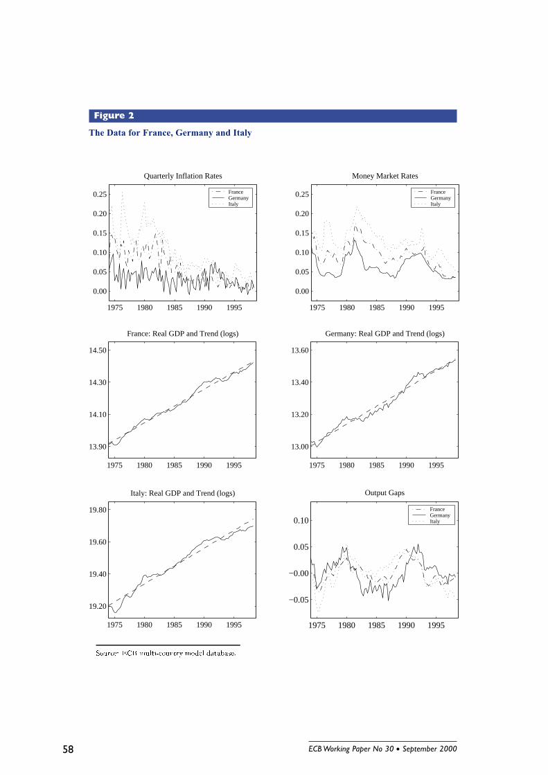
The source of the downward trend in euro area inflation noted previously is directly

apparent from Figure 2. As shown in the top left-hand panel inflation rates in the early

1970s were much higher in countries such as France and Italy than in Germany due to oil

price shocks and accommodative monetary policy. It took 10 to 15 years, respectively, for

French and Italian inflation rates to decline to German levels. Convergence in inflation

rates was accompanied by convergence in nominal interest rates in the late 1990s as can

be seen from the upper right-hand panel. Over time, as economic convergence and the

future formation of a monetary union became more widely expected the inflation premium

incorporated in Italian and French short-term nominal interest rates relative to German

rates eventually disappeared.

This convergence process and the role of the EMS in its context have been widely

debated and analyzed in the academic and policy literature of the last decade.14 There is

little doubt that the decline of inflation has largely been due to the growing commitment on

the part of monetary policy makers in the euro area to achieve and maintain low inflation.

The credibility of this commitment, however, likely varied over time, probably being rather

low in the early stages of the EMS in the early and mid 1980s and higher during the “hard”

EMS period in the late 1980s up to the EMS crises in 1992 and 1993. Following these

crises credibility regarding the central banks’ commitment to achieve low inflation likely

increased again with the progress of preparations for EMU. To the extent that disinflation

during these periods was credible and expected by wage and price setters, the associated13Other alternatives include estimates based on the HP filter or unobserved components methods. We

have conducted some sensitivity studies in this respect. We stick with the linear trend as our benchmark forcomparability with the results obtained by Fuhrer and Moore and Taylor for the U.S. and because of thesimilarity to the OECD estimate of the euro area output gap.

14For more detailed discussions of this convergence process see for example Gros and Thygesen (1992),Giavazzi and Pagano (1994), De Grauwe (1996, 1997), Favero et al. (1997), Angeloni and Dedola (1999).


output losses would have been rather low. In fact, a casual comparison of the extent of

disinflation in Italy and France relative to Germany and the output gap estimates for these

three economies based on the log-linear trends that are shown in the bottom right panel

of Figure 2, suggests that the disinflations in Italy and France did not require large and

protracted recessions and thus may have been partly anticipated.

In principle, a complete model of the European inflation process prior to EMU would

need to account for both, the long-run convergence process as well as the short-run variations

around this downward trend. However, modelling the convergence process would require

taking into account the varying degree of credibility of exchange rate pegs, the possibility

of crises and realignments and learning by market participants about the long-run inflation

objectives of European policymakers. Such an analysis would be beyond the objective of

this paper.

Instead we take a shortcut by approximating the implicit time-varying inflation objective

with a linear trend, and then estimate the overlapping contracts models using inflation

deviations from this trend. We detrend the average inflation rate for the euro area as well

as the French and Italian inflation rates in this manner. Similar approaches have been used

by other researchers with regard to European inflation data, notably Gerlach and Svensson

(1999) and Cecchetti, McConnell and Quiros (2000).15 As an additional robustness check

regarding our euro area estimates, we also consider the exponential trend preferred by

Gerlach and Svensson. Estimates of both the linear and the exponential trend are depicted

in the top left-hand panel of Figure 1. An advantage of the exponential trend estimate

is that it flattens out in the late 1990s and is consistent with stable average inflation from

then on. A drawback is the unreasonably high trend level of inflation at the beginning of

the sample.

Focusing on inflation deviations from trend would be appropriate, if the source of disin-15Gerlach and Svensson use an exponential trend for the euro area inflation rate in estimating a P-star

model of inflation dynamics a la Hallman, Porter and Small (1991) for the euro area. Cecchetti et al.construct inflation and output deviations from a 12-month moving average of actual values and estimateinflation-output tradeoffs based on this data for a number of euro area economies.


flation had been a credible, fully anticipated, gradually phased-in reduction in the policy-

makers’ inflation target. However, given this was not the case, this approach introduces an

error that may bias our estimation results. In particular, it could influence the estimated

degree of inflation persistence and the implied case for the relative real wage specification.

Again, the estimation with German data will provide a useful benchmark for comparison,

because it is the only case for which the inflation series exhibits no strong trend. In addition,

we will conduct a sensitivity study to assess how our euro area estimates would change if

market participants had been consistently surprised by the downward trend.

4 Empirical inflation and output dynamics

Our empirical analysis proceeds in two stages. In the first stage, we estimate an uncon-

strained bivariate VAR model of output and inflation. In the second stage, we use this

unconstrained VAR as an auxiliary model in estimating the structural overlapping wage

contracting specifications by simulation-based indirect inference methods. These are meth-

ods for calibrating the parameters of the structural model by matching its reduced form,

which constitutes a constrained VAR, as closely as possible with the estimated uncon-

strained VAR model.

The unconstrained VAR provides an empirical summary description of euro area infla-

tion and output dynamics.16 We estimate the short-run dynamics jointly with a determinis-

tic linear trend for inflation and the logarithm of output over the sample period. Following

Fuhrer and Moore (1995a) we then compute the autocorrelation functions implied by the

VAR including the associated asymptotic confidence bands.17 These autocorrelation func-

tions serve as an indication whether the lead-lag relationship between inflation and output

is consistent with a short-run tradeoff, that is, with a short-run Phillips curve. Furthermore,16Although interest rates are important determinants of output and inflation, we restrict attention to

bivariate VARs without including an interest rate, primarily because it is unclear what would be an appro-priate interest rate for the euro area. We return to this problem later on in section 6 when estimating anaggregate demand equation that closes the small macroeconomic model.

17For a detailed discussion of the methodology and the derivation of the asymptotic confidence bands forthe estimated autocorrelation functions the reader is referred to Coenen (2000).


they form a benchmark against which we can evaluate the ability of the alternative overlap-

ping contracts specifications to explain the dynamics of inflation in euro area data. Such an

approach has also been recommended by McCallum (1999), who argued that autocovariance

and autocorrelation functions are a more appropriate device for confronting macroeconomic

models with the data than impulse response functions because of their purely descriptive

nature.

The empirical model for output and inflation, written in terms of the level of inflation,

Πt, and the logarithm of output, Qt, corresponds to[Πt

Qt

]=

[a0,Π

a0,Q

]+

[a1,Π

a1,Q

]t +

[πt

qt

], (5)

where πt and qt refer to the inflation and the output gap respectively, which are determined

by an unconstrained VAR of lag order 3:[πt

qt

]= A1

[πt−1

qt−1

]+ A2

[πt−2

qt−2

]+ A3

[πt−3

qt−3

]+

[uπ,t

uq,t

]. (6)

The Ai matrices (i = 1, 2, 3) contain the coefficients on the first three lags of the inflation

and the output gap.18 The error terms uπ,t and uq,t are assumed to be serially uncorrelated

with mean zero and positive definite covariance matrix Σu.

We fit this model to the aggregated output and inflation data for the euro area as a

whole for the period from 1974:Q1 to 1998:Q4. First, we detrend the data by a simple

projection technique and then we estimate the parameters of the VAR model, that is the

coefficient matrices Ai and the covariance matrix Σu by Quasi-Maximum-Likelihood (QML)

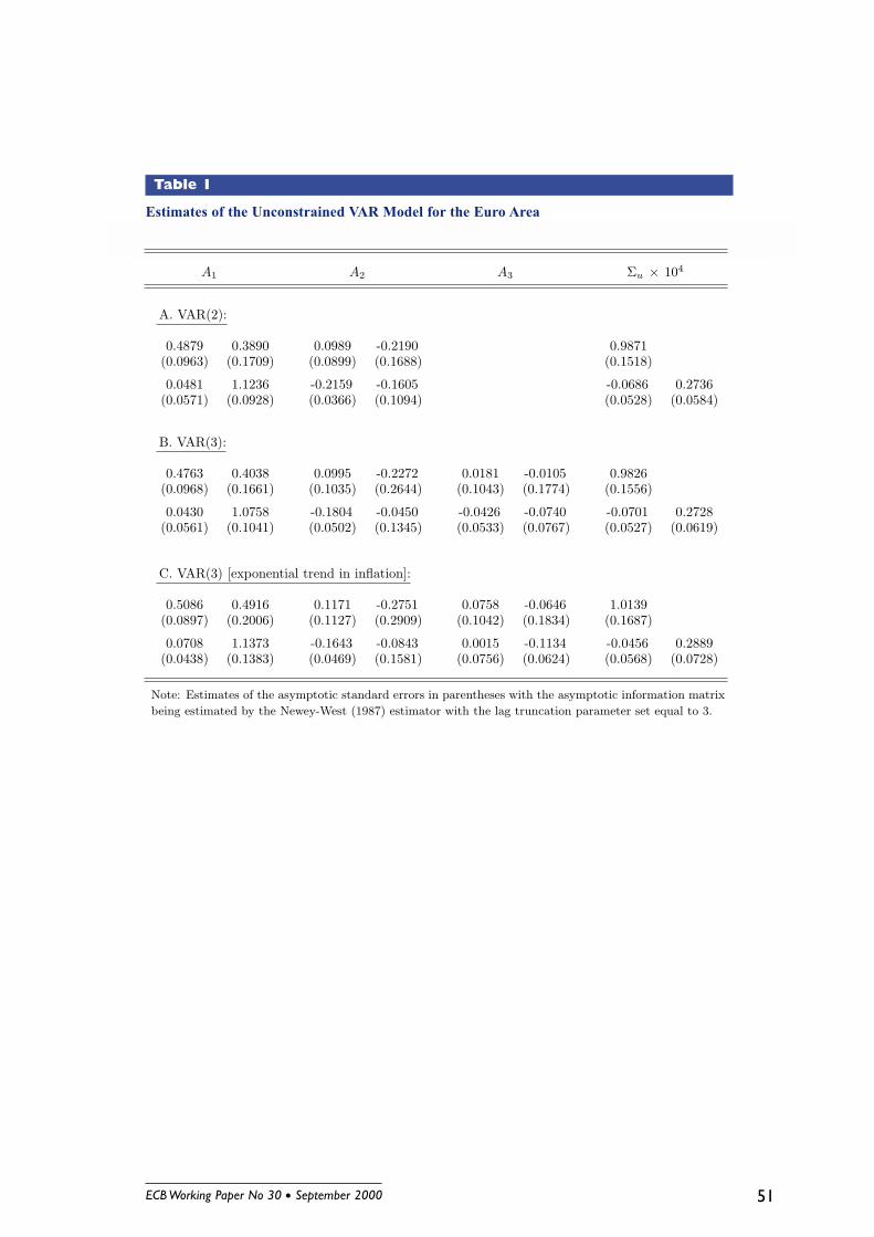
methods.19 The estimates of the unconstrained VAR model are shown in Table 1. Standard

lag selection procedures based on the HQ and SC criteria suggest that a lag order of 2 would

be sufficient to capture the empirical inflation and output dynamics. The Ljung-Box Q(12)

statistic indicates serially uncorrelated residuals with a marginal probability value of 42.8%.

The estimates of the parameters of the VAR(2) model are shown in panel A. Our point18Here, we use a maximum lag order of 3, simply because this corresponds to the reduced-form VAR

representation of the overlapping contract models of section 2 with a contract length of 4 quarters.19For some more detail the reader is referred to the appendix, section A.2.


estimates imply that the smallest root of the characteristic equation det(I2−A1 z−A2 z2) =

0 is 1.2835, thereby suggesting that the inflation and output gaps are stationary. This

conclusion is roughly supported by the results of standard univariate Dickey-Fuller tests for

the presence of unit roots.

We also estimate an unconstrained VAR(3) model. This is of interest, because all

contracting specifications discussed in section 2 have a reduced form which is a constrained

VAR of order 3 if the maximum contract length is one year. To assess the sensitivity of

our results to the lag length, we will use the VAR(2) and VAR(3) models in parallel in the

estimation of the contracting specifications in the following section. On a statistical basis,

the third lag would not be absolutely necessary, as can be seen from panel B, which shows

that the A3 coefficients are insignificant. As a further robustness check we also estimate a

VAR(3) model based on inflation deviations from the exponential trend. As can be seen

by comparing the estimates in panel B with those in panel C the VAR(3) coefficients differ

little between the linear trend and exponential trend specification, with the differences well

below one standard deviation.

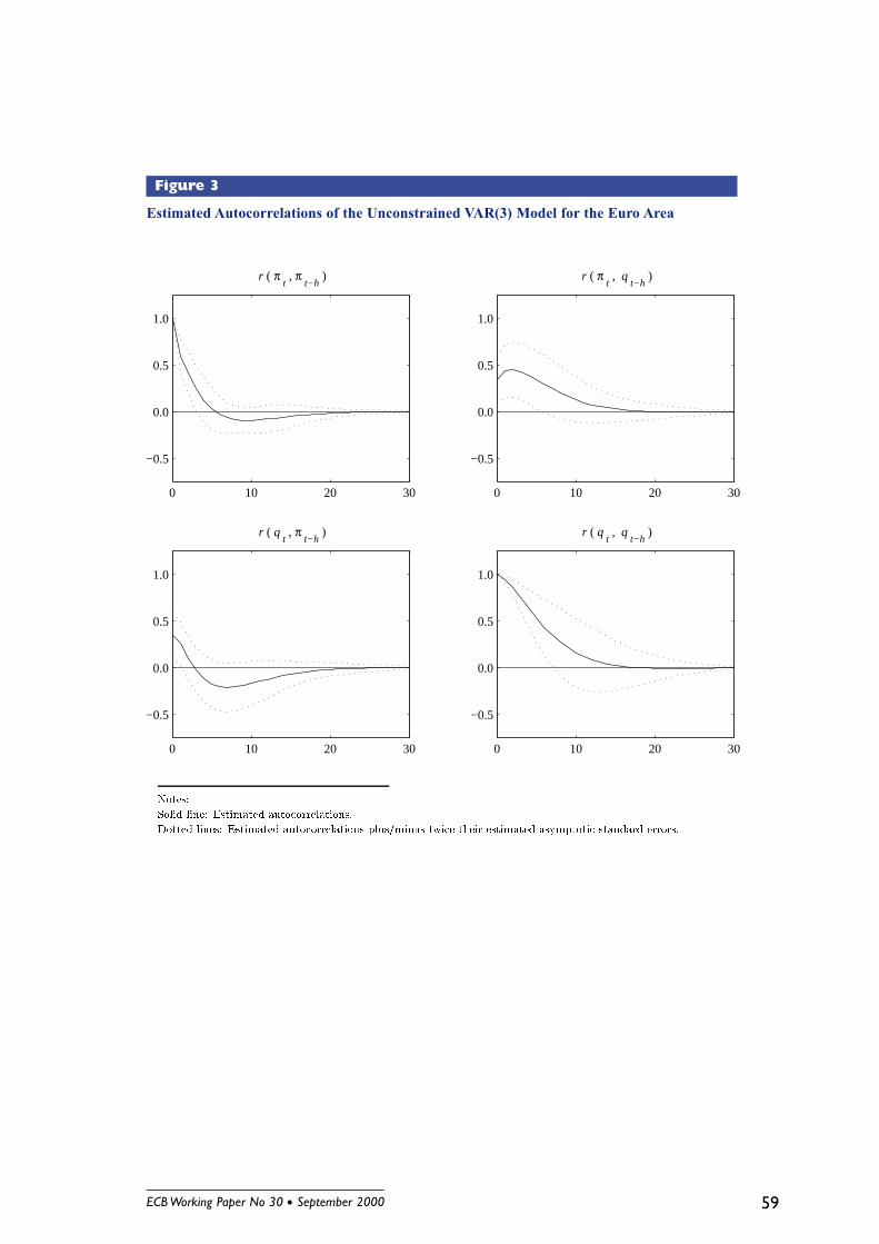
The autocorrelation functions associated with the unconstrained VAR(3) model of the

euro area based on the linear trend are depicted in Figure 3. The diagonal elements show

the autocorrelations of the detrended inflation rate and the output gap, the off-diagonal

elements the lagged cross correlations. The solid lines represent the point estimates, while

the dotted lines indicate 95% confidence bands. Both inflation and output are quite persis-

tent with positive autocorrelations out to lags of about 5 and 8 quarters which are highly

significant. The cross correlations in the off-diagonal panels confirm much of conventional

wisdom about inflation and output dynamics. For example, in the second panel of the top

row, a high level of output is followed by a high level of inflation a year later and again these

cross correlations are statistically significant. In the first panel of the bottom row a high

level of inflation is followed by a low level of output a year later. These lead-lag interactions

are highly indicative of the existence of a conventional short-run tradeoff between output

and inflation. All in all these correlations are stylized facts which any structural model of


output and inflation dynamics ought to be able to explain. The autocorrelation functions of

the VAR(3) model based on inflation deviations from the exponential trend are very similar

and thus not shown in the figure.

The results for the bivariate VARs of order 3 for France, Germany and Italy are sum-

marized in Table 2. Note that for Germany the estimates are obtained without a trend

in inflation (a1,Π = 0). The estimated autocorrelation functions for output and inflation

in France and Italy display qualitatively similar characteristics as for the euro area as a

whole, in particular regarding the persistence in inflation and output variations. The cross

correlations, however, are somewhat smaller.20 As to Germany, the degree of persistence

in inflation is substantially lower and the correlations between current output and lagged

inflation have the opposite sign, albeit statistically insignificant. We return to these issues

in the next section, when we use the empirical autocorrelation functions as a benchmark to

evaluate the fit of alternative structural overlapping contracts specifications.

5 Estimating the overlapping contracts specifications

In the following we use the unconstrained VAR models as approximating probability models

in estimating the coefficients of the different overlapping contracts specifications discussed

in section 2. As can be seen from equations (1) through (4) there are only three structural

parameters to estimate for each specification: (i) the slope of the contracting distribution

s that determines the series of contract weights fi; (ii) the sensitivity of the contract wage

to expected future aggegrate demand over the life of the contract γ; and (iii) the standard

deviation of the contract wage shock σεx .

5.1 The reduced-form representation

Of course, the overlapping contracts specifications discussed in section 2 do not represent a

complete model of inflation determination. Since the contract wage equations (2) and (4)20To save space, we do not report separate figures for the estimated autocorrelation functions and their

associated asymptotic confidence bands. They are plotted jointly with the autocorrelation functions of theconstrained VARs obtained under alternative overlapping contracting specifications in Figures 5, 6 and 7.


contain expected future output gaps, we need to specify how the output gap is determined

in order to solve for the reduced-form representation of inflation and output dynamics

under each of the contracting specifications. A full-information estimation approach would

require a complete macroeconomic model and estimate all the model’s structural parameters

jointly. A version of such a model in the spirit of Fuhrer and Moore (1995b) would include

an aggregate demand equation, which relates output gaps to ex-ante long-term real rates,

as well as a Fisher equation, a term structure relationship and a monetary policy rule.

While our ultimate objective is to build precisely such a model, we take a less ambi-

tious approach in estimating the contracting parameters. We simply use the output gap

equation from the unconstrained VAR models, which corresponds to the second row in (6),

as an auxiliary equation for output determination. This limited-information approach is

close to the estimation approaches used by Taylor (1993a) and Fuhrer and Moore (1995a)

and is likely to be more robust to specification errors in the part of the model describing

output determination than a full-information approach. We estimate the aggregate demand

equation later on by single-equation methods and discuss those results in the next section.

Using the output equation from the unconstrained VAR together with the wage-price

block from section 2, we can solve for the reduced-form inflation and output dynamics under

each of the four different contracting specifications (RW, RW-C, RW-S and NW).21 For this

purpose it is convenient to rewrite the wage-price block, which was originally defined in

levels of nominal contract wages and prices, in terms of the real contract wage (x−p)t

and the annualized quarterly inflation rate πt. The reduced-form solution of this rational

expectations model is a trivariate constrained VAR. While the quarterly inflation rate πt and

the output gap qt are observable variables, the real contract wage (x−p)t is unobservable.22

For a contracting specification with a one-year maximum contract length this constrained21We assume that the expectations in the contract wage equations are formed rationally, and use the

AIM algorithm of Anderson and Moore (1985) which solves for the reduced-form dynamics of linear rationalexpectations models by employing the Blanchard and Kahn (1980) method.

22Note that for some models such as the RW-C specification it is helpful to define further auxiliary statevariables that are unobservable. A more detailed discussion is provided in the appendix.


VAR can be written as (x−p)t

πt

qt

= B1

(x−p)t−1

πt−1

qt−1

+ B2

(x−p)t−2

πt−2

qt−2

+ B3

(x−p)t−3

πt−3

qt−3

+ B0 εt, (7)

where the Bi matrices (i = 0, 1, 2, 3) contain the coefficients of the constrained VAR and εt

is a vector of serially uncorrelated error terms with mean zero and positive (semi-) definite

covariance matrix which is assumed to be diagonal with its non-zero elements normalized

to unity.

The coefficients in the bottom row of the Bi matrices coincide exactly with the coeffi-

cients of the output equation of the unconstrained VAR, with the B0 cofficients obtained by

means of a Choleski decomposition of the covariance matrix Σu. The reduced-form coeffi-

cients in the upper two rows of the Bi matrices, which are associated with the determination

of the real contract wage and inflation, are functions of the structural parameters (s, γ, σεx)

as well as the coefficients of the output equation of the unconstrained VAR.

5.2 Estimates of the structural parameters

We estimate the structural parameters of the overlapping contracts specifications s, γ and

σεx using the indirect inference methods proposed by Smith (1993) and Gourieroux, Mon-

fort and Renault (1993) and developed further in Gourieroux and Monfort (1995, 1996).

The estimation procedure, including its asymptotic properties, is discussed in detail in the

appendix of this paper. In the appendix we also compare this procedure to the Maximum-

Likelihood methods used by Taylor (1993a) and Fuhrer and Moore (1995a).

Indirect inference is a simulation-based procedure for calibrating a structural model with

the objective of finding parameter values such that its dynamic characteristics match the

dynamic properties of the observed data as summarised by an approximating probability

model. The latter should fit the empirical dynamics reasonably well, but need not necessar-

ily nest the structural model. In the case at hand, the unconstrained VAR model discussed

in section 4 is a natural candidate for such an approximating probability model. By serving

as the approximating probability model for the estimation of the structural parameters by


indirect inference and by providing a summary description of the inflation and output gap

dynamics which the structural model should be able to explain the unconstrained VAR

model provides a single, consistent benchmark for the empirical analysis carried out in this

paper.

Of course, one cannot directly match the parameters of the constrained VAR model (7)

with the parameters of the unconstrained VAR model (6) because the constrained VAR

model also includes the unobservable real contract wage variable. Instead, for given values

of the structural parameters (s, γ, σεx) and the parameters of the output gap equation from

the unconstrained VAR model, we simulate the reduced form of the structural model, that

is the constrained VAR model, to generate “artificial” series for the real contract wage,

the inflation rate and the output gap. All that is needed for simulation are three initial

values for each of these variables and a sequence of random shocks.23 Subsequently we fit

the unconstrained VAR model to the artificial series of inflation and the output gap and

match the simulation-based estimates of the inflation equation as closely as possible with

the empirical estimates by searching over the feasible space of the structural parameters.24

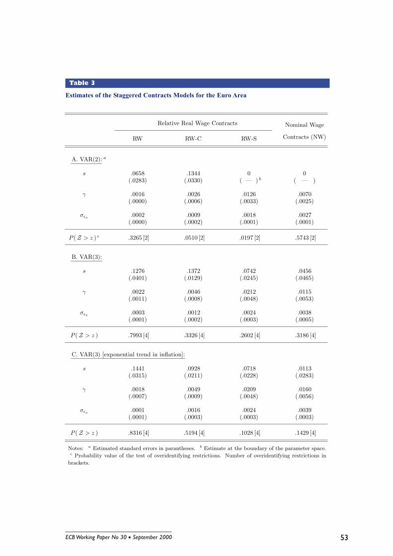
Euro area estimation results for the baseline version of the relative real wage contract-

ing model (RW), the version with price expectations conditioned on historically available

information (RW-C), the simplified version preferred by Fuhrer and Moore (RW-S) and the

nominal wage contracting model (NW) are reported in Table 3. As a sensitivity check

we consider both the VAR(2) and VAR(3) models estimated in section 4 as approximat-

ing probability models.25 Furthermore, we investigate whether our findings based on the

VAR(3) model are robust to the use of inflation deviations from the exponential instead of23In estimation we use steady-state values as initial conditions and are careful to only use simulation data

for later periods that are essentially unaffected by this choice of initial conditions. This issue is discussed inmore detail in the appendix, section A.3.

24We do not need data for the unobservable real contract wage since the unconstrained VAR is only fittedto the observable data for inflation and the output gap.

25In the case of the VAR(2) model, we restrict the maximum contract length in the structural contractingspecification to three quarters instead of one year, such that its lag order corresponds to that of the structuralmodel’s reduced-form solution. In this case, the slope parameter s is restricted to lie in the interval ( 0, 1/3 ].Note, because of the difference in its domain the magnitude of the slope parameter will not be directlycomparable across the specifications with three-quarter and one-year maximum contract length, respectively.


the linear trend. The estimation results indicate that all four contracting models fit the euro

area inflation dynamics reasonably well, in particular when we allow for a maximum con-

tract length of one year and thus three lags in the VAR. As can be seen from the standard

errors given in parentheses, the estimates of the structural parameters are in almost all cases

statistically significant, with the appropriate sign and economically significant magnitude.

We also compute the probability (P -) values of the test for the over-identifying re-

strictions, which were imposed when estimating the structural parameters. According to

this test, none of the four contracting specifications is rejected by the data, when we use

the VAR(3) as approximating probability model and allow for a one-year maximum con-

tract length. The coefficient estimates we obtain when using inflation deviations from the

exponential trend are with one exception within one standard deviation of the estimates

based on the linear trend in inflation. When we use the VAR(2) model and constrain the

maximum contract length to three quarters, both, the RW-C and the RW-S specification

can be rejected at convenient confidence levels, but not the RW or the NW specifications.

Though the estimates of the real wage contracting specifications are not directly compa-

rable, since the latter imply structures with different degrees of forward-lookingness, it is

worthwhile to note that the RW-S specification implies stronger rigidities than the RW and

the RW-C specifications as measured by the smaller estimates of the slope parameter s of

the contracting distributions.

While neither the RW nor the NW specification can be rejected, we can use the associ-

ated P -values of the test of overidentifying restrictions to discriminate between these two

specifications. In the case of our preferred setup with one-year maximum contract length

and the VAR(3) as approximating probability model, the RW specification implies a higher

P -value than the NW specification, whether we use inflation deviations from a linear or an

exponential trend. For the estimation based on the VAR(2) model, however, the NW spec-

ification entails a higher P -value. Overall, the RW specification with one-year maximum

contract length performs best. Thus, our findings for the euro area differ quite a bit from

the results in Fuhrer and Moore (1995a), who reject the nominal wage contracting model


for U.S. data and find that the RW-S specification fits U.S. inflation dynamics better than

the theoretically more plausible RW specification.

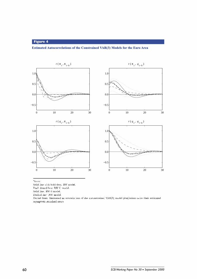
To provide further insight regarding these estimation results, we compare the autocor-

relation functions implied by the constrained VAR(3) representation of each of the four

contracting models with the autocorrelation functions from the unconstrained VAR. As

shown in Figure 4, the autocorrelation functions for all four models tend to remain inside

the 95% confidence bands (dotted lines) associated with the autocorrelation functions of the

unconstrained VAR. The three relative real wage contracting specifications (RW: solid line

with bold dots, RW-C: dash-dotted line, RW-S: solid line) are rather similar. They exhibit

substantial inflation persistence and quite pronounced cross correlations that are indicative

of a short-run Phillips curve tradeoff. The upper right-hand panel indicates that high levels

of output are followed by high inflation, while the lower left-hand panel shows that high

levels of inflation are followed by low levels of output. The only noticeable difference from

the unconstrained VAR is that the latter set of cross correlations are somewhat larger in

absolute magnitude for the constrained VAR. The autocorrelations for the nominal con-

tracting model (NW: dashed line) indicate a lower degree of inflation persistence and less

pronounced cross correlations than for the different relative real wage contracting models.

As noted in the introduction to this paper, the estimation results with euro area data

may be questioned for a number of reasons. First of all, the data are artificial in the

sense that they are only averages of the data from the member economies prior to the

formation of EMU. Furthermore, the member economies experienced different monetary

policy regimes. While Germany enjoyed stable inflation with fairly predictable monetary

policy, other countries such as France and Italy experienced a long-drawn out convergence

process, which was probably not fully anticipated by market participants. As a result,

euro area inflation data exhibits a longlasting decline which we removed from the data by

subtracting a linear trend.

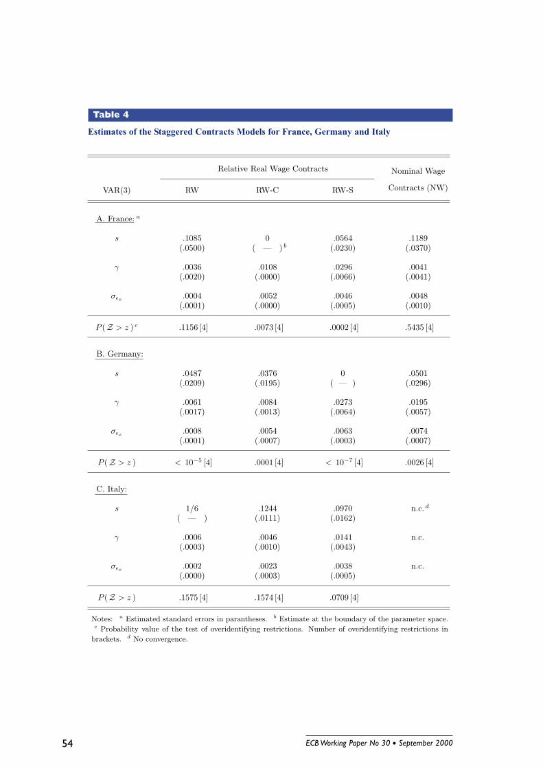
To investigate the validity of our results with respect to aggregation, we also estimate

the different contracting models for France, Germany and Italy separately. The results


are summarized in Table 4. Here we only focus on the case of the VAR(3) model. For

France we reject the RW-C and the RW-S specifications, but not the RW and the NW

specification. The NW model exhibits the highest P -value. However, in this case the

parameter measuring the sensitivity to aggregate demand, γ, is statistically insignificant.

The parameter estimates for the RW specification are significant and relatively close to

the values obtained for the euro area. For Italy, which experienced the most dramatic

transition process, the estimation of the NW model did not converge. Instead, the RW and

the RW-C model seem to fit Italian inflation data reasonably well and imply statistically

significant parameter estimates. For Germany, where inflation exhibited no long-run trend,

we find that all three relative real wage contracting models are strongly rejected by the

data. While the nominal contracting model is also rejected, it does fit better in the sense of

implying a higher P -value. The parameter estimates for the NW model with German data

are surprisingly close to the NW estimates obtained with euro area data.

Again, a promising alternative approach for evaluating the fit of the RW and NW spec-

ifications is to compare the autocorrelation functions of the constrained and unconstrained

VAR models. As shown in Figure 5 for France, the NW specification does better than the

RW specification in terms of fitting the empirical autocorrelations consistent with the result

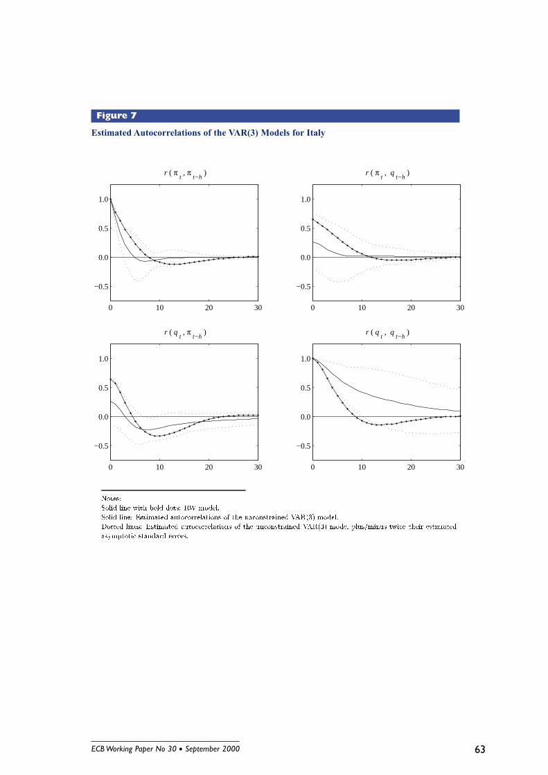
of the test of overidentifying restrictions presented in Table 4. In the case of Italy the RW

model comes close to matching the empirical autocorrelations of inflation in the top left-

hand panel of Figure 7, and also does reasonably well with regard to the cross correlations.

The results for Germany in Figure 6 are, as expected, quite different. The autocorrelation

functions of the unconstrained VAR (solid line with dotted confidence bands) indicated

a much smaller degree of inflation persistence and a counterintuitive, albeit statistically

insignificant, positive correlation between output and lagged inflation. Consequently, the

nominal contracting model has a better chance at fitting German inflation dynamics than

the relative contracting models.

We conclude from these results that, both the RW and the NW specifications are plau-

sible alternatives for the euro area. On the one hand, the estimation with aggregated euro


area data indicates a slight preference for the relative wage contracting model. On the

other hand, the comparison between France, Germany and Italy suggests that this prefer-

ence may partly be due to the high-inflation regime in countries such as Italy and France

and the fact that the subsequent long-run decline in inflation was not fully anticipated.

Thus, an optimist would conclude that the independent European Central Bank will likely

face a similar environment in the future as the Bundesbank did in Germany or possibly the

French central bank in the latter part of the EMS, that is in the “Franc fort” period. In

this case, the inflation-output relationship for the euro area would be best characterized by

the nominal contracting specification. A skeptic, who suspects that stabilizing euro area

inflation will require higher output losses, would instead prefer to use the RW specification

for the euro area. A robust monetary policy strategy, however, should perform reasonably

well under both specifications.

5.3 Further sensitivity analysis

As discussed in sections 3 and 4, we used inflation deviations from trend rather than the

inflation rate itself in estimating the alternative wage contracting specifications with French,

Italian and euro area data. In setting up the empirical VAR model in equations (5) and (6)

in section 4, we defined the inflation gap πt as the difference between the level of inflation

Πt and trend inflation. Throughout our analysis we used a linear trend but for the euro

area we considered in addition an exponential trend as a robustness check. The reason

for detrending inflation was to separate the short-run dynamics in inflation that are due

to nominal rigidities from the convergence process that was driven by changes in long-

run inflation objectives in countries such as France and Italy. The question remains how

our estimation results are affected by detrending the inflation series. Our approach would

have been correct if the cause of the long-run decline in inflation that is captured by this

trend would have been a fully anticipated and credible, gradually phased-in reduction in

the policymakers’ inflation target. However, given this was not the case, this approach

introduces an error that may bias our estimation results.


In order to assess whether the detrending procedure may have introduced a significant

error in our estimation, we have conducted a small Monte Carlo Study. In this study we

compare the small-sample properties of the indirect inference estimation procedure under

two alternative scenarios. The first scenario assumes that the downward linear trend in in-

flation was perfectly anticipated by wage and price setters. This scenario forms a benchmark

for comparison that is needed to determine the small sample properties of the estimation

procedure, when the model is correctly specified, before investigating the effect of model

mis-specification on those estimates. In the second scenario, we consider the more realistic

alternative that wage and price setters were consistently surprised by the downward trend

in inflation. Technically, this means we assume that wage and price setters expect trend

inflation to follow a random walk. Thus, denoting trend inflation by π∗, market partici-

pants expect trend inflation to be determined according to π∗t = π∗t−1 + επ∗,t, where επ∗

is a random shock. The motivation for this scenario is the following. Although market

participants were not able to perfectly predict the downward trend in inflation, they were

certainly able to take into account the possibility of unpredictable changes in the underlying

long-run inflation target of monetary policymakers.

First, we generate a large number of data samples under each of these two scenarios.

Then, we apply the detrending and estimation procedure to each simulated history. While

the estimation procedure is correct in the first scenario, it suffers from mis-specification in

the case of the random-walk scenario. We then assess to what extent the estimates ob-

tained under either of the two scenarios differ from the true parameter values. Of course,

the random-walk expectations scenario is only one of many possible scenarios, but it should

provide some indication whether detrending the inflation series induces a danger of signif-

icantly under- or overstating the degree of inflation persistence due to structural nominal

rigidities.

We decided to use the RW-S contracting specification for this Monte Carlo study, because

it induces the highest degree of inflation persistence. Specifically we use the parameter

estimates obtained with euro area data for the specification with a maximum contract


length of four quarters, i.e. s = 0.0742, γ = 0.0212 and σεx = 0.0024. The sample sizes

we consider are T ∈ { 100, 500 }. For each sample size 100 replications are carried out and

for each simulated sample 100 initial observations are discarded to minimize the effect of

the initial values that are set to the model’s steady-state values. For the simulations with

random walk expectations we draw the shocks επ∗ from a normal distribution with mean

-0.001 and a standard deviation of the same absolute magnitude. As a result the simulated

histories exhibit a negative drift, which on average is equal to the historical downward trend

in euro area inflation.

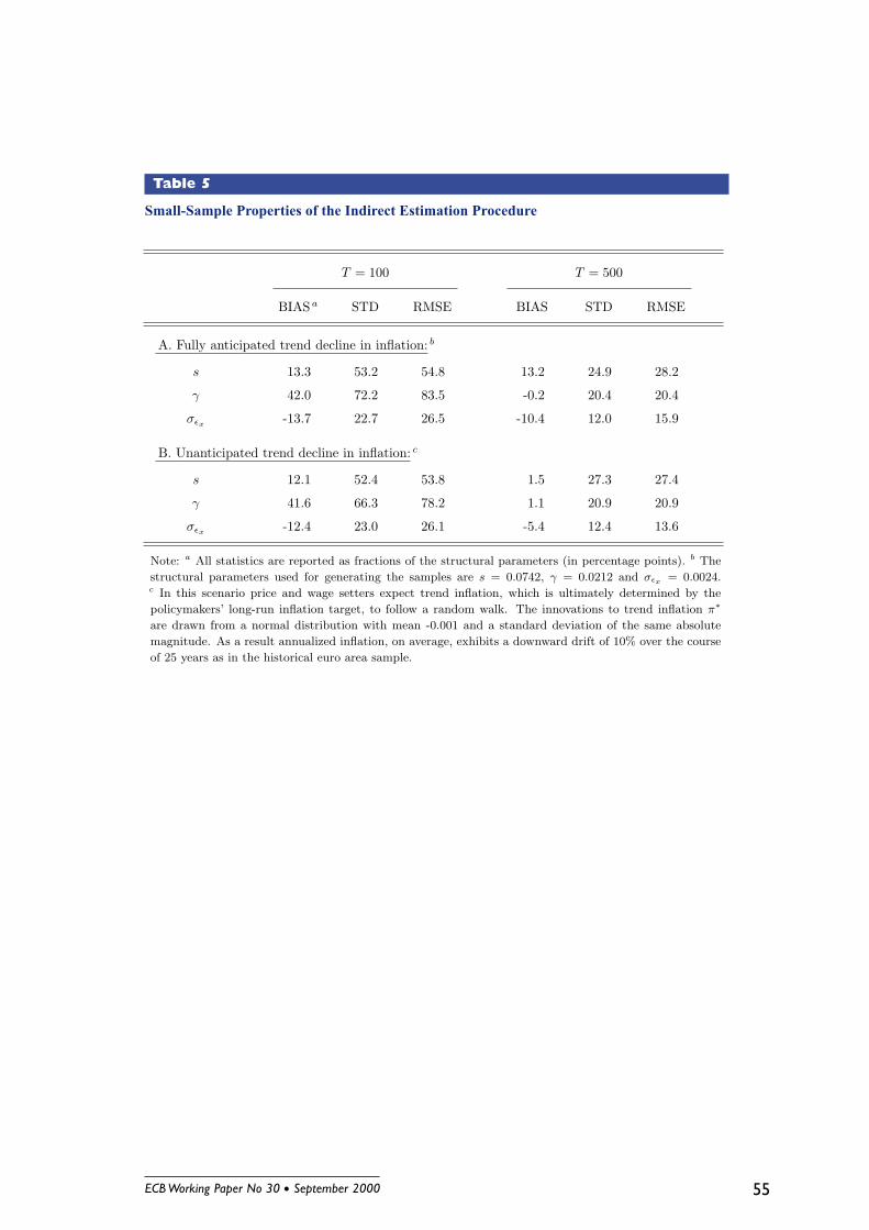
The small-sample performance of the simulation-based indirect estimator is evaluated by

means of some simple statistics: the average deviation of the estimates from the structural

parameters (s, γ, σεx) used for generating the data (BIAS), their standard deviation (STD)

and their root mean-squared error (RMSE). The statistics are expressed as fractions of

the structural parameters (reported in percentage points). The results of the Monte Carlo

experiment are summarized in Table 5.

Panel A refers to the baseline scenario where the downward trend in inflation is fully

anticipated by wage and price setters, that is, the case where our approach of detrending

the inflation series is correct. In this case, we find that with a sample size of T = 100 the

estimates of the slope parameter of the contracting distribution s are biased upwards by

13.3% on average. This means, the indirect estimation method somewhat under-estimates

the persistence of the inflation process in the RW-S model. The estimates of the sensitivity

of the contract wage to expected future aggregate demand γ are biased upwards by 42.0%

and the estimates of the standard deviation of the contract wage shock σεx are biased

downwards by -13.7%. Once we increase the sample size to T = 500 the biases of the

estimates and similarly their standard deviation and their root mean-squared error turn

out to be much smaller. We conclude from this exercise that our estimation procedure has

reasonably good small-sample properties at least when the underlying model is correctly

specified.

The outcome of the Monte Carlo study under the second scenario, where wage and price


setters’ expectations incorporate the possibility of unpredictable changes in trend inflation

(ultimately the policymaker’s long-run inflation target), is reported in panel B. Although,

the estimation procedure is still based on detrended inflation series and consequently not

fully appropriate, the biases, standard deviations and root mean squared errors of the

resulting parameter estimates are generally of the same magnitude as in panel A. In other

words, the error introduced by detrending the inflation series under this scenario is rather

small. In some cases the error even turns out to offset the small-sample bias observed in

panel A to some extent. For example, the biases regarding the estimates of s and σεx are

a bit smaller than in panel A. Thus, the assumption implicit in our estimation procedure,

namely that the downward-trend in inflation was fully anticipated by price setters, does

not seem to introduce significant distortions in our estimation. While this is only a limited

sensitivity study, we find the outcome rather encouraging.

Given the estimates of euro area inflation dynamics, as reported in Table 3, we now

proceed to close the model by estimating an aggregate demand equation and imposing a

term structure relationship and an interest rate rule.

6 Closing the model: Output gaps and interest rates

We model aggregate demand with a simple reduced-form IS equation, which relates the

current output gap, qt, to two lags of itself and to the lagged long-term ex-ante real interest

rate, rlt−1:

qt = δ0 + δ1 qt−1 + δ2 qt−2 + δ3 rlt−1 + σεd

εd,t. (8)

εd,t denotes an unexpected demand shock scaled with the parameter σεd, which measures

the standard deviation of the demand shock. The rationale for including lags of output is

to account for habit persistence in consumption as well as adjustment costs and accelerator

effects in investment. We use the lagged instead of the contemporaneous value of the real

interest rate to allow for a transmission lag of monetary policy. For now we neglect the

possibility of effects of the real exchange rate and expected future income on aggregate


demand. Fuhrer and Moore (1995b) found that a similar aggregate demand specification

fits U.S. output dynamics quite well. Since the euro area is a large, relatively closed economy

just like the United States, the exchange rate is likely to play a less important role than it

did in the individual member economies prior to EMU.

Next we turn to the financial sector and relate the long-term ex-ante real interest rate,

which affects aggregate demand, to the short-term nominal interest rate, which is the prin-

cipal instrument of monetary policy. Three equations determine the various interest rates

in the model. The short-term nominal interest rate, ist , is set according to a Taylor-type

interest rate rule (see Taylor (1993b)). This rule incorporates policy responses to inflation

deviations from target and output deviations from potential output, and allows for some

degree of partial adjustment:

ist = αr ist−1 + (1− αr)(r∗ + π(4)t ) + απ(π(4)

t − π∗) + αq qt. (9)

r∗ denotes the long-run equilibrium real rate, while π∗ refers to the policymaker’s target

for inflation. The inflation measure is the four-quarter moving average of the annualized

quarterly inflation rate, that is π(4)t = 1

4

∑3j=0 πt−j = pt − pt−4, and the interest rate is

annualized.

As to the term structure, we rely on the accumulated forecasts of the short rate over two

years which, under the expectations hypothesis, will coincide with the long rate forecast for

this horizon:

ilt = Et

18

7∑j=0

ist+j

, (10)

where the term premium is assumed to be constant and equal to zero. By subtracting

inflation expectations over the following 8 quarters, we then obtain the long-term ex-ante

real interest rate:

rlt = ilt − Et

[12(pt+8 − pt)

]. (11)

To estimate the parameters of the aggregate demand equation (8) we first construct the

ex-post real long-term rate as defined by equations (10) and (11) but replacing expected


future with realized values. We then proceed to estimate the parameters by means of Gen-

eralized Method of Moments (GMM) using lagged values of output, inflation and interest

rates as instruments. The estimation results are reported in Table 6. The sample period

for this estimation is 1974:Q4 to 1997:Q1.

Panel A refers to the estimates for the euro area. In the first row, the output gap and

interest rate data are area-wide GDP-PPP-weighted averages. The coefficients on the two

lags of the output gap are significant and exhibit an accelerator pattern. The interest rate

sensitivity of aggregate demand has the expected negative sign, however the parameter

estimate is only borderline significant and rather small. It is not clear however, what is

the appropriate real interest rate measure for the euro area. For example, instead of GDP

weights it may be a more appropriate to use the relative weights in debt financing for

aggregating national nominal interest rates. Or, one could make the argument that the

relevant real rate for the euro area is the German one. After all, movements in German

interest rates presumably had to be mirrored eventually by the other countries to the

extent that they intended to maintain exchange rate parities within the European Monetary

System. For this reason we also use the German real interest rate to estimate the interest

rate sensitivity of euro area aggregate demand. In this case, as shown in the second row,

we find similar coefficients on the lags of the output gap, but the estimate of the interest

rate sensitivity is highly significant and three times as large.

We have subjected this specification of aggregate demand to a battery of sensitivity

tests. For example, we have investigated alternative specifications of potential output,

alternative horizons on the term structure equation, including the use of average long-term

rates instead of a term structure based on short-term rates and we have varied the length

of the sample period. At least qualitatively the estimation results remain the same.

For comparison, we have also estimated the same specification for France, Germany and

Italy. In each case we use the domestic real interest rate. For France and Italy we obtain

qualitatively similar estimates as for the euro area. For Germany however, the estimate

of the interest rate sensitivity is not significant and the lags of output do not exhibit an


accelerator-type pattern.

It remains to discuss the deterministic steady state of this model. In steady state,

the output gap is zero and the long-term real rate is equal to the equilibrium real rate,

r∗. This equilibrium rate is determined as a function of the parameters of the aggregate

demand curve (8), given by r∗ = −δ0/δ3. The steady-state value of inflation is determined

exclusively by monetary policy. Since the overlapping contracts specifications of the wage-

price block do not impose any restriction on the steady-state inflation rate, steady-state

inflation will be equal to the inflation target, π∗, in the policy rule.

7 Evaluating monetary policy rules: An example

In the last few years it has become quite common to represent alternative monetary policy

strategies in terms of rules for setting the short-term nominal interest rate. As far as Eu-

ropean countries are concerned, empirical work by Clarida and Gertler (1997) and Clarida,

Galı and Gertler (1998) suggests that German interest rate policy since 1979 is summarized

quite well by an interest rate rule that responds to the forecast of inflation and the current

output gap and exhibits some degree of partial adjustment. Clarida et al. (1998) also argue

that German monetary policy had a strong influence on interest rate policy in the U.K.,

France and Italy throughout this period and may have led to higher interest rates in those

countries than warranted by domestic conditions at the time of the EMS collapse.26 More

recently, Gerlach and Schnabel (2000) have suggested that average interest rates in the

EMU countries in 1990-98, with the exception of the period of exchange market turmoil in

1992-93, moved very closely with average output gaps and inflation as implied by Taylor’s

rule.

In the remainder of this section we explore the inflation and output dynamics that would

arise in our model of the euro area when the coefficients in the interest rate rule (9) are set

equal to the values proposed in Taylor (1993b), that is αr = 0, απ = 0.5 and αq = 0.5. To

this end, we simulate the impulse responses of inflation and output to unexpected demand26For an analysis of these tensions based on a multi-country model see Wieland (1996).


and supply shocks as well as a disinflation. We compare the simulation outcomes with the

euro area estimates of the RW, RW-S, RW-C and NW specifications as well as the German

estimate of the NW specification. For euro area aggregate demand we use the estimates

obtained with the German real interest rate as reported in the second row of Table 6.

We start with an unexpected temporary supply shock, which in our framework is a

shock to the contract wage equation. The standard deviation of this type of shock, σεx ,

was estimated as part of the structural estimation of each of the contracting specifications

in section 5. The effect of a standard deviation contract wage shock when policy follows

Taylor’s rule is depicted in Figure 8. The top and bottom left-hand panels show the

response of inflation and the output gap given euro area estimates of the three different

relative real wage contracting specifications. The solid line with bold dots refers to the

RW specification, which we found to fit best with euro area data. The RW-S and RW-C

specifications correspond to the solid and dashed-dotted lines respectively.

The shock occurs in the first quarter of the second year (period 5). As a result of

this shock inflation increases over the next four quarters by almost a full percentage point.

Monetary policy, which follows Taylor’s rule, responds to this increase in inflation by raising

short-term nominal interest rates sufficiently so as to increase the long-term real interest

rate. This policy tightening induces a slowdown in aggregate demand which lasts for about

four years. Since future aggregate demand affects contract wage setting and through this

channel the inflation rate, inflation returns back to target after little more than two years

and even undershoots for a few periods thereafter.

The panels on the right-hand side of Figure 8 report the inflation and output responses

for the nominal wage contracting specifications for Germany (dashed line) and the euro

area (dotted line). Qualitatively, the impact on output and inflation is the same as for the

relative wage contracting specifications. For the German estimates the impact on inflation

is of similar magnitude, while it is somewhat smaller with the euro area estimates. Of

course, the differences between the latter two simulations may partly be due to differences

in the parameters of aggregate demand. The important result is that the magnitude of the


shortfall of aggregate demand is much smaller under the nominal wage specifications than

under the relative real wage specifications. Thus, the cost of stabilizing inflation in terms

of reduced output is much larger under the relative real wage specifications.

Figure 9 reports output and inflation responses in the case of an unexpected temporary

demand shock of 0.5 percentage points of potential output. Again the outcomes under the

relative real wage contracting specifications are shown in the panels on the left and under

nominal wage contracting on the right-hand side. As demand increases above potential,

inflation also rises above target up to 1 percentage point under the RW and RW-C specifi-

ciations. The impact on inflation is somewhat smoother but more drawn out for the RW-S

specification. Monetary policy responds to this increase in inflation and output by raising

nominal interest rates sufficiently to induce an increase in the long-term real interest rate

which reduces aggregate demand and ultimately returns both inflation and output to steady

state. Comparing the relative real wage contracting specifications with the nominal wage

contracting specification, it is directly apparent that the inflationary impact of the demand

shock is much smaller under nominal contracting.

Finally, Figure 10 reports the effect of a disinflation by 2 percentage points under the

alternative contracting specifications. This disinflation is simulated as an unanticipated,

perfectly credible change in the policymaker’s inflation target, π∗ in the policy rule (9),

from 2 percent to 0 percent. Initial conditions are consistent with a steady-state inflation

rate of 2 percent. As shown in the two right-hand side panels, inflation declines rather

quickly, within a year, to the new target value when contract wages are set according to

Taylor’s nominal contracting model. This decline is only accompanied by very small output

losses. The solid lines in the left-hand side plane indicate that the output losses necessary to

achieve this disinflation is much higher when contract wages are set according to the RW-S

specification preferred by Fuhrer and Moore (1995a). A more surprising finding, however,

is that the cost of disinflation under the RW and the RW-C specifications (solid line with

bold dots and dashed-dotted line) is much lower than under the RW-S specification. In

fact it is not too different from the disinflation in the NW model. The reason for the lower


output cost of the disinflation is that wage setters in the RW and RW-C setup set contract

wages with respect to the average price level expected to prevail over the life of the contract.

In the RW-S model contract wages are instead set with respect to the current price level.

Thus, wage setters in the RW and RW-C models more quickly incorporate the disinflation

in their decisions.

As far as future European monetary policy is concerned, however, the disinflation sce-

nario shown in Figure 10 may not be as relevant, simply because euro area inflation was

already below the ECB’s upper threshold of 2 percent at the outset of monetary union.

Instead, the more relevant question may be how to keep inflation low in the event of un-

foreseen shocks such as the temporary demand and supply shocks depicted in Figures 8

and 9 respectively.

8 Summary and concluding remarks

We have estimated a small-scale empirical model of the euro area where short-run real effects

of monetary policy arise due to overlapping wage contracts. In particular, we focused on

the nominal wage contracting model due to Taylor (1980) and three different versions of

the relative real wage contracting model first proposed by Buiter and Jewitt (1981) and

investigated empirically by Fuhrer and Moore (1995a) for the United States. Contrary to

Fuhrer and Moore, who reject the nominal contracting model and find strong evidence in

favor of the relative contracting model which induces a higher degree of inflation persistence,

we find that both types of contracting models fit euro area data reasonably well. The best

fitting specification is a version of the relative contracting model, which is theoretically

more plausible than the simplified version preferred by Fuhrer and Moore.

To investigate the validity of our results, we also estimated the contracting models for

France, Germany and Italy separately. Our findings show that the relative contracting

model does quite well in countries which transitioned out of a high inflation regime such as

France and Italy, while the nominal contracting model fits German data better.

One interpretation of these findings is that nominal rigidities in wage and price setting


are more pronounced in countries such as France and Italy than in Germany. If so, one

might expect that the euro area as a whole will also be characterized by a higher degree of

nominal rigidity than in Germany as suggested by our estimates based on euro area averages.

Another interpretation would attribute the higher degree of inflation persistence in euro

area, French and Italian data to expectations about imperfectly credible monetary policy

and less than fully anticipated disinflation. In this case, the better fit of the relative wage

contracting specification would be considered misleading. And consequently, the nominal

wage contracting model may be viewed as a more accurate measure of nominal rigidities in

the euro area in the future.

We close the model by estimating aggregate demand equations and positing a term

structure relationship as well as a policy rule. Using the response coefficients recommended

by Taylor (1993b) in this policy rule, we investigate the impact of unexpected demand and

price shocks on output and inflation. As expected, we find that stabilizing inflation in the

event of adverse price shocks is much more costly under the relative real wage contract-

ing specifications than the nominal contracting specification. Furthermore, unanticipated

demand shocks have a much stronger inflationary impact in the relative wage contracting

models. The findings for unanticipated, credible disinflations are more surprising, since only

one of the relative real wage specifications requires a substantial output loss to achieve such

a disinflation.

For future research on evaluating alternative monetary policy strategies for the euro area

with this model we plan to use both, the best fitting relative real wage and nominal wage

contracting specifications. Given the high degree of uncertainty about the determination of

euro area inflation in the future, it seems particularly important to identify robust monetary

policy strategies that perform reasonably well under different types of nominal rigidities.


References

Amato, J. and T. Laubach, 1999, Monetary policy in an estimated optimization-basedmodel with sticky prices and wages, Manuscript.

Anderson, G. S. and G. R. Moore, 1985, A linear algebraic procedure for solving linearperfect foresight models, Economics Letters, 17, 247-252.

Angeloni, I. and L. Dedola, 1999, From the ERM to the euro: New evidence on economicand policy convergence among EU countries, European Central Bank, Working Paper No.4, May.

Angeloni, I., V. Gaspar and O. Tristani, 1999, The monetary policy strategy of the ECB,in D. Cobham and G. Zis (eds.), From EMS to EMU, London: Macmillan.

Ascari, G. and J. A. Garcia, 1999, Relative wage concern and the Keynesian contractmultiplier, EUI Working Paper ECO No. 99/5.

Blanchard, O. J. and C. Kahn, 1980, The solution of linear difference models under rationalexpectations, Econometrica, 48, 1305-1311.

Branch, M. A. and A. Grace, 1996, Optimization toolbox: For use with MATLAB, Natick:The Math Works.

Brayton, F., A. Levin, R. W. Tryon and J. C. Williams, 1997, The evolution of macro modelsat the Federal Reserve Board, Carnegie-Rochester Conference Series on Public Policy, 42,115-167.

Bryant, R. C., P. Hooper and C. Mann (eds.), 1993, Evaluating policy regimes: New researchin empirical macroeconomics, Washington DC: Brookings Institution.

Buiter, W. H. and I. Jewitt, 1981, Staggered wage setting with real wage relativities: Vari-ations on a theme of Taylor, The Manchester School, 49, 211-228, reprinted in W. H. Buiter(ed.), 1989, Macroeconomic theory and stabilization policy, Manchester: Manchester Uni-versity Press.

Cecchetti, S., M. McConnell and G. Perez Quiros, 2000, Policymakers’ revealed prefer-ences and the output-inflation variability tradeoff: Implications for the European Systemof Central Banks, forthcoming, European Economic Review.

Clarida, R. and M. Gertler, 1997, How the Bundesbank conducts monetary policy, in C.Romer and D. Romer (eds.), Reducing inflation, Chicago: NBER and University of ChicagoPress.

Clarida, R., J. Galı and M. Gertler, 1998, Monetary policy rules in practice: Some interna-tional evidence, European Economic Review, 42, 1033-1067.


Clarida, R., J. Galı and M. Gertler, 1999, The science of monetary policy: A new Keynesianperspective, Journal of Economic Literature, 37, 1661-1707.

Clarida, R., J. Galı and M. Gertler, 2000, Monetary policy rules and macroeconomic sta-bility: Evidence and some theory, Quarterly Journal of Economics, 115, 147-180.

Coenen, G., 2000, Asymptotic confidence bands for the estimated autocovariance and au-tocorrelation functions of vector autoregressive models, European Central Bank, WorkingPaper No. 9, January.

De Grauwe, P., 1996, Inflation convergence during the transition to EMU, in P. De Grauwe,S. Micossi and G. Tullio (eds.), Inflation and wage behaviour in Europe, Oxford: OxfordUniversity Press.

De Grauwe, P., 1997, The economics of monetary integration, 3rd edition, Oxford: OxfordUniversity Press.

Duffie, D. and K. J. Singleton 1993, Simulated moments estimation of Markov models ofasset prices, Econometrica, 61, 929-952.

Erceg, C., D. Henderson, and A. Levin, 1999, Optimal monetary policy with staggered wageand price contracts, forthcoming in Journal of Monetary Economics.

Fagan, G., J. Henry and R. Mestre, 1999, An area-wide model (AWM) for the EU11,European Central Bank, Manuscript.

Fair, R. C. and E. P. Howrey, 1996, Evaluating alternative monetary policy rules, Journalof Monetary Economics, 38, 173-193.

Favero, C. A., F. Giavazzi and L. Spaventa, 1997, High yields: the spread on Germaninterest rates, Economic Journal, 107, 956-985.

Fuhrer, J. C., 1997, Inflation/output variance trade-offs and optimal monetary policy, Jour-nal of Money, Credit, and Banking, 29, 214-234.

Fuhrer, J. C. and G. R. Moore, 1995a, Inflation persistence, Quarterly Journal of Economics,110, 127-159.

Fuhrer, J. C. and G. R. Moore, 1995b, Monetary policy trade-offs and the correlationbetween nominal interest rates and real output, American Economic Review, 85, 219-239.

Galı, J. and M. Gertler, 1999, Inflation dynamics: A structural econometric analysis, Jour-nal of Monetary Economics, 44, 195-222.

Gallant, R. A. and G. Tauchen, 1996, Which moments to match?, Econometric Theory, 12,657-681.

Giavazzi, F. and M. Pagano, 1994, The advantage of tying one’s hands: EMS discipline and


central bank credibility, in T. Persson and G. Tabellini (eds.), Monetary and fiscal policy,Volume 1, Credibility, Cambridge: MIT Press (previously published in 1988, EuropeanEconomic Review, 32, 1055-1075).

Gerlach, S. and L. E. O. Svensson, 1999, Money and inflation in the euro area: A case formonetary indicators?, Manuscript, July.

Gerlach, S. and G. Schnabel, 2000, The Taylor rule and interest rates in the EMU area,Economics Letters, 67, 165-171.

Goodfriend, M. and R. King, 1997, The new neoclassical synthesis and the role of monetarypolicy, NBER Macroeconomics Annual, Cambridge: MIT Press.

Gourieroux, C. and A. Monfort, 1995, Testing, encompassing and simulating dynamic econo-metric models, Econometric Theory, 11, 195-228.

Gourieroux, C. and A. Monfort, 1996, Simulation-based inference methods, Oxford: OxfordUniversity Press.

Gourieroux, C., A. Monfort and E. Renault, 1993, Indirect inference, Journal of AppliedEconometrics, 8, Special issue: Econometric inference using simulation techniques, S85-S118.

Gros, D. and N. Thygesen, 1992, European monetary integration, London: Longman.

Hallman, J. J., R. D. Porter and D. H. Small, 1991, Is the price level tied to the M2aggregate in the long run?, American Economic Review, 81, 841-858.

McCallum, B. T., 1999, Analysis of the monetary transmission mechanism: methodologicalissues, Manuscript, June.

McCallum, B. T. and E. Nelson, 1999, Performance of operational policy rules in an esti-mated semiclassical structural model, in Taylor, 1999a.

Newey, W. K. and K. D. West, 1987, A simple, positive semi-definite, heteroskedasticityand autocorrelation consistent covariance matrix, Econometrica, 55, 703-708.

OECD, 1999, OECD economic outlook No. 65, Organisation for Economic Co-Operationand Development, June.

Orphanides, A, D. Small, V. Wieland and D. Wilcox, 1997, A quantitative exploration ofthe opportunistic approach to disinflation, Finance and Economics Discussion Series, 97-36,Board of Governors of the Federal Reserve System, June.

Orphanides, A. and V. Wieland, 1998, Price stability and monetary policy effectivenesswhen nominal interest rates are bounded at zero, Finance and Economics Discussion Series,98-35, Board of Governors of the Federal Reserve System, June.


Reifschneider, D., R. Tetlow and J. C. Williams, 1999, Aggregate disturbances, Monetarypolicy, and the macroeconomy: The FRB/US perspective, Federal Reserve Bulletin, 85,1-19.

Roberts, J., 1997, Is inflation sticky?, Journal of Monetary Economics, 39, 173-196.

Rotemberg, J. and M. Woodford, 1997, An optimization-based econometric framework forthe evaluation of monetary policy, NBER Macroeconomics Annual, Cambridge: MIT Press.

Rotemberg, J. and M Woodford, 1999, Interest-rate rules in an estimated sticky price model,in Taylor, 1999a.

Rudebusch, G. and L. E. O. Svensson, 1999, Policy rules for inflation targeting, in Taylor,1999a.

Sbordone, A., 1998, Price and unit labor costs: A new test of price stickiness, Manuscript,August.

Smith, A. A., 1993, Estimating nonlinear time-series models using simulated vector autore-gressions, Journal of Applied Econometrics, 8, Special issue: Econometric inference usingsimulation techniques, S63-S84.

Toda, H. Y. and T. Yamamoto, 1995, Statistical inference in vector autoregressions withpossibly integrated processes, Journal of Econometrics, 66, 225-250.

Taylor, J. B., 1980, Aggregate dynamics and staggered contracts, Journal of Political Econ-omy, 88, 1-24.

Taylor, J. B., 1993a, Macroeconomic policy in the world economy: From econometric designto practical operation, New York: W.W. Norton.

Taylor, J. B., 1993b, Discretion versus policy rules in practice, Carnegie-Rochester Confer-ence Series on Public Policy, 39, 195-214.

Taylor, J. B. (ed.), 1999a, Monetary policy rules, Chicago: NBER and University of ChicagoPress.

Taylor, J. B., 1999b, Low inflation and the pricing power of firms, Manuscript, October.

White, H., 1994, Estimation, inference and specification analysis, Cambridge: CambridgeUniversity Press.

Wieland, V., 1996, Monetary policy targets and the stabilization objective: A source oftension in the EMS, Journal of International Money and Finance, 15, 95-116.


A Estimation by indirect inference

To estimate the structural parameters of the overlapping contracts specifications we applythe indirect inference methods proposed by Smith (1993), Gourieroux, Monfort and Renault(1993) and developed further in Gourieroux and Monfort (1995, 1996). Indirect inference isa simulation-based procedure for calibrating a structural model with the objective of findingvalues of its parameters such that its dynamic characteristics match the dynamic propertiesof the observed data as summarized by the estimated parameters of an approximatingprobability model.27 The latter should fit the empirical dynamics reasonably well, but neednot necessarily nest the structural model. The unconstrained VAR model, which we usedas a descriptive device to explore the dynamic interaction of the inflation and output datain section 4 is a natural candidate for such an approximating probability model.

We start with a brief review of standard Maximum-Likelihood (ML) methods usedby Taylor (1993a) and Fuhrer and Moore (1995a) for estimating the structural models athand in subsection A.1, and then motivate and describe the indirect estimation method insubsection A.2. We also discuss the asymptotic properties of the indirect estimator as wellas a global specification test which may be used to assess whether the structural model isconsistent with the data. Finally, subsection A.3 provides more detail on the implementationof the indirect estimation method.

A.1 The ML estimator

Both, the Taylor and Fuhrer-Moore models have a stationary reduced-form vector autore-gressive representation

zt = B1 zt−1 + · · ·+ Bp zt−p + B0 εt, (A.1)

where the K-dimensional vector of endogenous variables zt = [ x′t, y′t ]′ comprises a k-dimensional vector of observable variables yt and a (K − k)-dimensional vector of non-observable variables xt such as the contract wage. The K-dimensional vector εt is seriallyuncorrelated with mean zero and positive semi-definite covariance matrix. The covariancematrix is assumed to be diagonal with its non-zero elements normalized to unity. The(K × K)-dimensional coefficient matrices Bi = Bi(θ) (i = 0, 1, . . . , p) are non-linear func-tions of an m-dimensional vector of structural parameters θ ∈ Θ, where Θ ⊂ Rm denotesthe feasible parameter space. The maximum lag length p of the endogenous variables zt isequal to the maximum length of the wage contracts minus one. We refer to (A.1) as ourconstrained VAR(p) model, but also note that it contains unobservable variables such asthe contract wage xt in addition to output and inflation which are the only variables in theempirical VAR.

27See Duffie and Singleton (1993) and Gallant and Tauchen (1996) for related approaches relying eitheron selected sample moments or on the scores of an approximating probability model.


The reduced-form representation of the structural model can also be characterized by afamily of parametric conditional density functions

F(θ) ={

f(z−p+1, . . . , z0; θ), { f(yt |zt−p, . . . , zt−1; θ) }∞t=1 : θ ∈ Θ}

where f(θ) denotes an element of F(θ). The observed data { yt }Tt=−p+1 is then presumed to

be a sample from f(z−p+1, . . . , z0; θ)∏T

t=1 f(yt | zt−p, . . . , zt−1; θ) for some θ ∈ Θ. Usually,the structural parameter vector θ may be estimated by Maximum-Likelihood (ML) methodsrelying on Kalman filtering techniques (see Fuhrer and Moore (1995a, 1995b)). In particular,if we condition on fixed pre-sample values z−p+1, . . . , z0, the conditional ML estimator θT

for θ is

θT = arg maxθ∈Θ

T∑t=1

ln f(yt |zt−p, . . . , zt−1; θ).

Under appropriate regularity conditions the ML estimator θT is consistent for the “true”structural parameter vector θ0,

plimT→∞

θT = θ0,

and asymptotically normal,

√T (θT − θ0)

d−→ N[0,Σθ(θ0)],

where Σθ(θ0) is the asymptotic covariance matrix of√

T (θT − θ0).In practice, however, the ML estimator may be sensitive with respect to the choice

of the partially unobserved initial conditions z−p+1, . . . , z0 and may lack robustness if thepresumed data-generating process f(θ) is mis-specified.

A.2 The Indirect Estimator

Instead of estimating the parameter vector θ of the structural model directly, indirect es-timation starts from an approximating probability model – henceforth auxiliary model –which is capable of summarizing the dynamic characteristics of the sequence of observeddata { yt }T

t=−p+1.In the case at hand, we use the unconstrained k-dimensional VAR(p) model

yt = A1 yt−1 + · · ·+ Ap yt−p + ut (A.2)

with ut being serially uncorrelated with mean zero and positive-definite covariance matrixE[utu

′t] = Σu for approximating the structural model, because the latter has a constrained

VAR(p) representation as given by (A.1).


Throughout, we assume that the unconstrained VAR(p) model (A.2) is stable, i.e.

det( Ik −A1 z − · · · −Ap zp ) = 0 ⇒ | z | > 1,

where | · | denotes the absolute value operator.The unconstrained VAR(p) model, in turn, can be characterized by a parametric family

of conditional densities

F(β) ={

f(y1−p, . . . , y0;β), { f(yt |yt−p, . . . , yt−1;β) }∞t=1 : β ∈ B}

with an element of F(β) being denoted by f(β) and where

β =[vec(A1, . . . , Ap)′, vech(Σu)′

]′,

is the n-dimensional parameter vector of the auxiliary VAR(p) model with n = pk2 + k(k +1)/2). B ⊂ Rn denotes the feasible parameter space. The vec( · )-operator stacks thecolumns of a matrix in a column vector and the vech( · )-operator stacks the elements onand below the principal diagonal of a square matrix.

Given a sample { yt }Tt=1 with fixed pre-sample values y−p+1, . . . , y0, its dynamic char-

acteristics can be summarized by computing the conditional Quasi-Maximum-Likelihood(QML) estimator βT for β,28

βT = arg maxβ∈B

T∑t=1

ln f(yt |yt−p, . . . , yt−1;β).

Under general regularity conditions the QML estimator βT is consistent for the “true”reduced-form parameter vector β0,

plimT→∞

βT = β0,

and asymptotically normal,√

T (βT − β0)d−→ N[0,Σβ(β0)],

28As layed out in Section 4, we assume that the available data {Yt }Tt=−p+1 are a sample of the 2-

dimensional vector of variables Y = [Π, Q ]′ being generated by the linear model

Yt = α0 + α1 t + yt

with { yt } following a stable VAR(p) process as represented by (A.2) above. This type of model has beenadvocated by Toda and Yamamoto (1995) for conducting statistical inference in vector autoregressions withpossibly integrated variables.

Substituting (A.2), it becomes obvious that {Yt } is assumed to follow a VAR(p) process around a deter-ministic linear trend,

Yt − α0 − α1 t = A1 (Yt−1 − α0 − α1 (t − 1)) + · · · + Ap (Yt−p − α0 − α1 (t − p)) + ut.

Since we are merely interested in the parameters of the VAR(p) model, i.e. A1, . . . , Ap and Σu, we proceedin two steps. First, we detrend the data by a simple projection technique to obtain the sample { yt }. Second,using this sample, we compute the QML estimates of the parameters of interest.


where Σβ(β0) = H(β0)−1I(β0)H(β0)−1 is the asymptotic covariance matrix of√

T (βT−β0).I(β0) denotes the asymptotic information matrix and H(β0) is the asymptotic expectedHessian of the appropriately normalized quasi-log-likelihood function evaluated at β0.29

If the auxiliary model F(β) approximates the structural model F(θ) sufficiently well, itmakes sense to estimate the vector of structural parameters θ indirectly by minimizing the“distance” between the structural model F(θ) and the auxiliary model fitted to the data,i.e. f(βT ) ∈ F(β). Thus, the indirect estimator brings the information in βT to bear on thetask of estimating the structural parameter vector θ.

To make this approach operational Gourieroux, Monfort and Renault (1993) andGourieroux and Monfort (1995, 1996) start from the well-known Kullback-Leibler infor-mation criterion (KLIC),

KLIC(β, θ) = E θ

[ln

(f(yt|zt−p, . . . , zt−1; θ)f(yt|yt−p, . . . , yt−1;β)

)],

and introduce the so-called binding function b: Θ → B,

b(θ) = arg minβ∈B

KLIC(β, θ)

= arg maxβ∈B

E θ

[ln f(yt|yt−p, . . . , yt−1;β)

],

which, for a given θ ∈ Θ, identifies the density f(β) ∈ F(β) minimizing the distance betweenthe particular density f(θ) ∈ F(θ) and the elements of the family of densities F(β).

For a given β ∈ B, the expectation of the logarithm of the conditional densityln f(yt|yt−p, . . . , yt−1;β) has to be determined with respect to the conditional densityf(yt|zt−p, . . . , zt−1; θ) from f(θ) ∈ F(θ). While this expectation cannot be obtained an-alytically in general, it may easily be approximated for given parameters θ and β by thesimulated sample moment

1S

S∑s=1

ln f(ys(θ)|ys−p(θ), . . . , ys−1(θ);β),

where the simulated sample { ys(θ) }Ss=−p+1 is generated by the structural model character-

ized by f(θ) ∈ F(θ).Obviously, the approximation of the binding function b(θ) coincides with the QML

estimator βS(θ) of the auxiliary model using the simulated sample,

βS(θ) = arg maxβ∈B

1S

S∑s=1

ln f(ys(θ)|ys−p(θ), . . . , ys−1(θ);β),

where, without loss of generality, the simulated conditional quasi-log-likelihood function hasbeen normalized by 1/S.

29See White (1994) for a thorough treatment of QML theory and covariance estimation.


Subsequently, a simulation-based indirect estimator θS,T for θ is obtained by minimizinga criterion function QS,T : B × Θ → R+ which is defined as a quadratic form measuringthe distance between the empirical QML estimator βT and the simulated QML estimatorβS(θ):

θS,T = arg minθ∈Θ

QS,T (βT , θ)

with

QS,T (βT , θ) =(

βT − βS(θ))′

WT (βT )(

βT − βS(θ))

,

where WT (βT ) is a positive definite (n × n)-dimensional weighting matrix which possiblydepends on the QML estimate βT . The two subscripts S and T indicate that the partic-ular object depends on both the empirical sample { yt }T

t=−p+1 and the simulated sample{ ys(θ) }S

s=−p+1.

Under appropriate assumptions, the following results can be established.

Proposition: (Asymptotic properties of the indirect estimator)

i. The indirect estimator θS,T is consistent for θ0,

plimT→∞

θS,T = θ0,

and asymptotically normal,√

T (θS,T − θ0)d−→ N[0, (1 + c−1)(B′W B)−1B′W Σβ W B (B′W B)−1],

where S = c T with c ∈ N, B = B(θ0) = (∂ / ∂θ′) b(θ0), Σβ = Σβ(β0) =limT→∞Var[

√T (βT − β0)] and W = W (β0) = plimT→∞WT (βT ) with β0 =

plimT→∞ βT .

ii. The asymptotically efficient indirect estimator θ ∗S,T is obtained by using a consistent

estimate(

Σβ,T

)−1of the optimal asymptotic weighting matrix W ∗ = Σ−1

βand is

asymptotically normal,√

T (θ ∗S,T − θ0)d−→ N[0, (1 + c−1)(B′Σ−1

βB)−1].

iii. If the auxiliary model F(β) nests the structural model f(θ0) ∈ F(θ), then the asymp-totically efficient indirect estimator θ ∗S,T is as efficient as the ML estimator θT .

iv. Under the null hypothesis that the structural model f(θ0) ∈ F(θ) is correctly specified,the statistic

ZS,T (βT , θ ∗S,T ) =S T

S + TQ ∗

S,T (βT , θ ∗S,T )


with

Q ∗S,T (βT , θ ∗S,T ) = min

θ∈Θ

(βT − βS(θ)

)′ (Σβ,T

)−1 (βT − βS(θ)

),

is asymptotically χ2-distributed with n−m degrees of freedom.

Proof: Parts i., ii. and iv. of the proposition are alternatively established in Smith (1993),Gourieroux, Monfort and Renault (1993) and Gourieroux and Monfort (1996), chapter 4.5.Part iii. follows from Gallant and Tauchen (1996), pp. 665-666.

Among the assumptions underlying this proposition is the identification condition thatthe equation b(θ) = β0 has a unique root at θ0 ∈ Θ. This condition resembles the standardidentification condition in a non-linear equation system. The necessary (order and rank)condition for identification is n ≥ m. If n > m holds, n − m overidentifying restrictionsare imposed when estimating θ. For the asymptotically efficient indirect estimator θ ∗S,T

these overidentifying restrictions can be tested by means of the statistic ZS,T (βT , θ ∗S,T ). Itsprobability value P (Z > z) gives the probability that the re-scaled minimized criterionfunction takes a value larger than that obtained in the estimation exercise. Hereby, aprobabilistic assessment of the consistency of the structural model and the data is obtained.

A.3 Implementation

To estimate the parameters of the different wage contracting specifications, it is necessaryto close the model in a way that makes it possible to solve for expected future output gaps.Rather than specifying a complete macroeconomic model for forecasting future output gapsthat enter the contract wage equations, we instead use the reduced-form output gap equationfrom the unconstrained VAR(p) model fitted to the data. Thus, we confine ourselves to theparameters of the inflation equation in conducting indirect inference. This approach is verymuch in the spirit of the limited-information ML procedure applied by Fuhrer and Moore(1995a). They use the output gap and interest rate equations from a three-dimensional VARmodel to generate the output gap forecasts in the relative real wage contracting equation.Similarly, Taylor (1993a) used such a reduced-form output gap equation in applying limited-information ML methods for estimating the structural parameters of the nominal wagecontracting equation.

Let S denote the ( (pk+1)×(pk2+k(k+1)/2) )-dimensional (0, 1) selection matrix whichpicks the elements of β ∈ B corresponding to the inflation equation, then our asymptoticallyefficient indirect estimator θ ∗S,T for θ ∈ Θ is obtained by minimizing the criterion function

Q ∗S,T (βT , θ) =

(βT − βS(θ)

)′S ′(S Σβ,T S

′)−1

S(

βT − βS(θ))

,

where βT and βS(θ) are the empirical and the simulated QML estimates of the parameters


of the unconstrained VAR(p) model and (Σβ,T )−1 is a consistent estimate of the optimalasymptotic weighting matrix W ∗ = (Σβ)−1.

In order to minimize the criterion function Q ∗S,T (βT , θ) with respect to θ ∈ Θ, we rely

on the sequential dynamic programming algorithm provided by the MATLAB Optimiza-tion Toolboox.30 This algorithm allows to take account of the constraints to be imposedon the parameter space Θ, thereby guaranteeing the existence of a unique rational expec-tations solution. When minimizing Q ∗

S,T (βT , θ), we repeatedly have to simulate samplesof the observable variables { ys(θ) }S

s=−p+1 from our structural model in order to computethe simulated QML estimate βS(θ). These samples are generated by drawing a normallydistributed random sequence { εs }S

s=−(p+p)+1 and recursively computing the accompany-ing sequences of endogenous variables { zs(θ) }S

s=−(p+p)+1 by using the structural model’sreduced-form representation (A.1) for varying parameter vectors θ ∈ Θ. The recursions maystart from arbitrary initial values z, but a sufficiently large number of simulated values, sayp = 100 − p, should be discarded in order to guarantee that the effect of the initial valuesdie out. The sequences of the observable variables { ys(θ) }S

s=−p+1 are subsequently retainedfrom the sequences { zs(θ) }S

s=−p+1. Note that in repeated simulations the employed ran-dom number generator must always start from the same random seed. Similarly, alwaysthe same initial values z must be chosen.

Reporting standard errors for the indirect estimate θ ∗S,T requires estimation of theasymptotic covariance matrix Σθ∗ = (1 + c−1)(B′ S ′ (S Σβ S

′)−1S B)−1. This matrix maybe consistently estimated by replacing the unknown quantities by consistent estimates,

Σθ∗,S,T = (1 + c−1)(

BS(θ∗S,T )′ S ′(S Σβ,T S

′)−1

S BS(θ∗S,T ))−1

with BS(θ) = (∂/∂θ′) βS(θ) being computed by finite difference methods.Our experience has been, however, that it is more convenient to estimate the asymptotic

covariance matrix by the inverse of the appropriately normalized Hessian of the criterionfunction that is returned by the numerical algorithm,

Σθ∗,S,T = (1 + c−1)

(12

∂Q ∗S,T (βT , θ ∗S,T )

∂θ ∂θ′

)−1

.

30See Branch and Grace (1996) for technical details.



Table 1

Estimates of the Unconstrained VAR Model for the Euro Area

A1 A2 A3 Σu × 104

A. VAR(2):

0.4879 0.3890 0.0989 -0.2190 0.9871(0.0963) (0.1709) (0.0899) (0.1688) (0.1518)

0.0481 1.1236 -0.2159 -0.1605 -0.0686 0.2736(0.0571) (0.0928) (0.0366) (0.1094) (0.0528) (0.0584)

B. VAR(3):

0.4763 0.4038 0.0995 -0.2272 0.0181 -0.0105 0.9826(0.0968) (0.1661) (0.1035) (0.2644) (0.1043) (0.1774) (0.1556)

0.0430 1.0758 -0.1804 -0.0450 -0.0426 -0.0740 -0.0701 0.2728(0.0561) (0.1041) (0.0502) (0.1345) (0.0533) (0.0767) (0.0527) (0.0619)

C. VAR(3) [exponential trend in inflation]:

0.5086 0.4916 0.1171 -0.2751 0.0758 -0.0646 1.0139(0.0897) (0.2006) (0.1127) (0.2909) (0.1042) (0.1834) (0.1687)

0.0708 1.1373 -0.1643 -0.0843 0.0015 -0.1134 -0.0456 0.2889(0.0438) (0.1383) (0.0469) (0.1581) (0.0756) (0.0624) (0.0568) (0.0728)

Note: Estimates of the asymptotic standard errors in parentheses with the asymptotic information matrix

being estimated by the Newey-West (1987) estimator with the lag truncation parameter set equal to 3.


Table 2

Estimates of the Unconstrained VAR(3) Model for France, Germany and Italy

A1 A2 A3 Σu × 104

A. France:

0.4898 0.4551 -0.0645 -0.4035 0.1262 0.0506 3.1883(0.1201) (0.3697) (0.1465) (0.5265) (0.0990) (0.3305) (0.6399)

0.0069 1.1412 -0.0804 -0.0661 0.0291 -0.1499 -0.2390 0.3151(0.0274) (0.1135) (0.0384) (0.1496) (0.0415) (0.0889) (0.1020) (0.0524)

B. Germany:

0.0334 0.4474 0.2035 -0.0508 0.1402 -0.1270 3.5367(0.0873) (0.1867) (0.0990) (0.2240) (0.0899) (0.2125) (0.4390)

-0.0190 0.7480 -0.1061 0.1380 -0.0197 0.0692 -0.2614 1.1826(0.0658) (0.0812) (0.0561) (0.0891) (0.0622) (0.0901) (0.2357) (0.1623)

C. Italy:

0.7137 0.5620 -0.0715 -0.5580 0.0074 0.0502 4.4426(0.1186) (0.3391) (0.2425) (0.7027) (0.0986) (0.4881) (1.1728)

0.0005 1.3220 -0.0215 -0.3212 -0.0711 -0.0362 0.2931 0.4077(0.0313) (0.1312) (0.0367) (0.1855) (0.0273) (0.0877) (0.1389) (0.0848)

Note: Estimates of the asymptotic standard errors in parentheses with the asymptotic information matrix

being estimated by the Newey-West (1987) estimator with the lag truncation parameter set equal to 3.


Relative Real Wage Contracts Nominal Wage

RW RW-C RW-S Contracts (NW)

A. VAR(2): a

s .0658 .1344 0 0(.0283) (.0330) ( — ) b ( — )

γ .0016 .0026 .0126 .0070(.0000) (.0006) (.0033) (.0025)

σεx .0002 .0009 .0018 .0027(.0000) (.0002) (.0001) (.0001)

P (Z > z ) c .3265 [2] .0510 [2] .0197 [2] .5743 [2]

B. VAR(3):

s .1276 .1372 .0742 .0456(.0401) (.0129) (.0245) (.0465)

γ .0022 .0046 .0212 .0115(.0011) (.0008) (.0048) (.0053)

σεx .0003 .0012 .0024 .0038(.0001) (.0002) (.0003) (.0005)

P (Z > z ) .7993 [4] .3326 [4] .2602 [4] .3186 [4]

C. VAR(3) [exponential trend in inflation]:

s .1441 .0928 .0718 .0113(.0315) (.0211) (.0228) (.0283)

γ .0018 .0049 .0209 .0160(.0007) (.0009) (.0048) (.0056)

σεx .0001 .0016 .0024 .0039(.0001) (.0003) (.0003) (.0003)

P (Z > z ) .8316 [4] .5194 [4] .1028 [4] .1429 [4]

Notes: a Estimated standard errors in parantheses. b Estimate at the boundary of the parameter space.c Probability value of the test of overidentifying restrictions. Number of overidentifying restrictions in

brackets.

Table 3

Estimates of the Staggered Contracts Models for the Euro Area


Relative Real Wage Contracts Nominal Wage

VAR(3) RW RW-C RW-S Contracts (NW)

A. France: a

s .1085 0 .0564 .1189(.0500) ( — ) b (.0230) (.0370)

γ .0036 .0108 .0296 .0041(.0020) (.0000) (.0066) (.0041)

σεx .0004 .0052 .0046 .0048(.0001) (.0000) (.0005) (.0010)

P (Z > z ) c .1156 [4] .0073 [4] .0002 [4] .5435 [4]

B. Germany:

s .0487 .0376 0 .0501(.0209) (.0195) ( — ) (.0296)

γ .0061 .0084 .0273 .0195(.0017) (.0013) (.0064) (.0057)

σεx .0008 .0054 .0063 .0074(.0001) (.0007) (.0003) (.0007)

P (Z > z ) < 10−5 [4] .0001 [4] < 10−7 [4] .0026 [4]

C. Italy:

s 1/6 .1244 .0970 n.c. d

( — ) (.0111) (.0162)

γ .0006 .0046 .0141 n.c.(.0003) (.0010) (.0043)

σεx .0002 .0023 .0038 n.c.(.0000) (.0003) (.0005)

P (Z > z ) .1575 [4] .1574 [4] .0709 [4]

Notes: a Estimated standard errors in parantheses. b Estimate at the boundary of the parameter space.c Probability value of the test of overidentifying restrictions. Number of overidentifying restrictions in

brackets. d No convergence.

Table 4

Estimates of the Staggered Contracts Models for France, Germany and Italy


Table 5

Small-Sample Properties of the Indirect Estimation Procedure

T = 100 T = 500

BIAS a STD RMSE BIAS STD RMSE

A. Fully anticipated trend decline in inflation: b

s 13.3 53.2 54.8 13.2 24.9 28.2

γ 42.0 72.2 83.5 -0.2 20.4 20.4

σεx-13.7 22.7 26.5 -10.4 12.0 15.9

B. Unanticipated trend decline in inflation: c

s 12.1 52.4 53.8 1.5 27.3 27.4

γ 41.6 66.3 78.2 1.1 20.9 20.9

σεx-12.4 23.0 26.1 -5.4 12.4 13.6

Note: a All statistics are reported as fractions of the structural parameters (in percentage points). b The

structural parameters used for generating the samples are s = 0.0742, γ = 0.0212 and σεx = 0.0024.c In this scenario price and wage setters expect trend inflation, which is ultimately determined by the

policymakers’ long-run inflation target, to follow a random walk. The innovations to trend inflation π∗

are drawn from a normal distribution with mean -0.001 and a standard deviation of the same absolute

magnitude. As a result annualized inflation, on average, exhibits a downward drift of 10% over the course

of 25 years as in the historical euro area sample.


Table 6

Estimates of the IS Curve for the Euro Area, France, Germany and Italy

δ0 δ1 δ2 δ3 σεd× 104 P (J > j ) b

A. Euro Area: a

A.1 area-wide rate: 0.0012 1.2347 -0.2737 -0.0364 0.3185 0.1209 [5](0.0007) (0.0916) (0.1004) (0.0224)

A.2 German rate: 0.0027 1.1807 -0.2045 -0.0947 0.3176 0.2307 [5](0.0012) (0.1006) (0.1065) (0.0333)

B. France: 0.0024 1.2247 -0.2708 -0.0638 0.3460 0.1977 [5](0.0008) (0.1275) (0.1284) (0.0234)

C. Germany: 0.0012 0.7865 0.1395 -0.0365 1.2289 0.2518 [5](0.0027) (0.0686) (0.0825) (0.0874)

D. Italy: 0.0023 1.3524 -0.3852 -0.0544 0.3913 0.4210 [5](0.0009) (0.0845) (0.0804) (0.0236)

Notes: a GMM estimates using a vector of ones and lagged values of the output gap (qt−1, qt−2), the

quarterly inflation rate (πt−1, πt−2, πt−3), and the short–term nominal interest rate (ist−1, ist−2, i

st−3) as

instruments. The weighting matrix is estimated by means of the Newey-West (1987) estimator with the

lag truncation parameter set equal to 7. Estimated standard errors in parantheses. b Probability value

of the J -test of overidentifying restrictions. Number of overidentifying restrictions in brackets.


Figure 1

The Euro Area Data

1975 1980 1985 1990 1995

0.00

0.05

0.10

0.15

Quarterly Inflation Rate and Trend

Linear Trend Exponential Trend

1975 1980 1985 1990 1995

0.00

0.05

0.10

0.15

Money Market Rate

1975 1980 1985 1990 1995

13.50

13.70

13.90

14.10

Real GDP and Trend (logs)

1975 1980 1985 1990 1995

−0.04

−0.02

0.00

0.02

0.04

Output Gap

TrendOECD

Source: ECB area-wide model database (see Fagan et al. (1999)). Aggregation over data for the member countries

of the euro area using �xed GDP weights at PPP rates. The OECD output gap is obtained by interpolating the

annual �gures reported in OECD (1999).


Figure 2

The Data for France, Germany and Italy

1975 1980 1985 1990 1995

0.00

0.05

0.10

0.15

0.20

0.25

Quarterly Inflation Rates

France GermanyItaly

1975 1980 1985 1990 1995

0.00

0.05

0.10

0.15

0.20

0.25

Money Market Rates

France GermanyItaly

1975 1980 1985 1990 1995

13.90

14.10

14.30

14.50

France: Real GDP and Trend (logs)

1975 1980 1985 1990 1995

13.00

13.20

13.40

13.60

Germany: Real GDP and Trend (logs)

1975 1980 1985 1990 1995

19.20

19.40

19.60

19.80

Italy: Real GDP and Trend (logs)

1975 1980 1985 1990 1995

−0.05

−0.00

0.05

0.10

Output Gaps

France GermanyItaly

Source: ECB multi-country model database.


Figure 3

Estimated Autocorrelations of the Unconstrained VAR(3) Model for the Euro Area

0 10 20 30

−0.5

0.0

0.5

1.0

r ( π t , π

t−h )

0 10 20 30

−0.5

0.0

0.5

1.0

r ( π t , q

t−h )

0 10 20 30

−0.5

0.0

0.5

1.0

r ( q t , π

t−h )

0 10 20 30

−0.5

0.0

0.5

1.0

r ( q t , q

t−h )

Notes:

Solid line: Estimated autocorrelations.

Dotted lines: Estimated autocorrelations plus/minus twice their estimated asymptotic standard errors.


Figure 4

Estimated Autocorrelations of the Constrained VAR(3) Models for the Euro Area

0 10 20 30

−0.5

0.0

0.5

1.0

r ( π t , π

t−h )

0 10 20 30

−0.5

0.0

0.5

1.0

r ( π t , q

t−h )

0 10 20 30

−0.5

0.0

0.5

1.0

r ( q t , π

t−h )

0 10 20 30

−0.5

0.0

0.5

1.0

r ( q t , q

t−h )

Notes:

Solid line with bold dots: RW model.

Dash-dotted line: RW-C model.

Solid line: RW-S model.

Dashed line: NW model.

Dotted lines: Estimated autocorrelations of the unconstrained VAR(3) model plus/minus twice their estimated

asymptotic standard errors.


Figure 5

Estimated Autocorrelations of the VAR(3) Models for France

0 10 20 30

−0.5

0.0

0.5

1.0

r ( π t , π

t−h )

0 10 20 30

−0.5

0.0

0.5

1.0

r ( π t , q

t−h )

0 10 20 30

−0.5

0.0

0.5

1.0

r ( q t , π

t−h )

0 10 20 30

−0.5

0.0

0.5

1.0

r ( q t , q

t−h )

Notes:



Solid line: Estimated autocorrelations of the unconstrained VAR(3) model.




Figure 6

Estimated Autocorrelations of the VAR(3) Models for Germany

0 10 20 30

−0.5

0.0

0.5

1.0

r ( π t , π

t−h )

0 10 20 30

−0.5

0.0

0.5

1.0

r ( π t , q

t−h )

0 10 20 30

−0.5

0.0

0.5

1.0

r ( q t , π

t−h )

0 10 20 30

−0.5

0.0

0.5

1.0

r ( q t , q

t−h )

Notes:







Figure 7

Estimated Autocorrelations of the VAR(3) Models for Italy

0 10 20 30

−0.5

0.0

0.5

1.0

r ( π t , π

t−h )

0 10 20 30

−0.5

0.0

0.5

1.0

r ( π t , q

t−h )

0 10 20 30

−0.5

0.0

0.5

1.0

r ( q t , π

t−h )

0 10 20 30

−0.5

0.0

0.5

1.0

r ( q t , q

t−h )

Notes:






Figure 8

Contract Wage Shock [+1 Standard Deviation]

Relative Real Wage Contracts Nominal Wage Contracts

5 10 15 20 25 30

−0.005

0.000

0.005

0.010

Inflation

5 10 15 20 25 30

−0.005

0.000

0.005

0.010

Inflation

5 10 15 20 25 30

−0.0025

0.0000

0.0025

Output Gap

5 10 15 20 25 30

−0.0025

0.0000

0.0025

Output Gap

Notes:

Solid line with bold dots: Euro area RW model.

Solid line: Euro area RW-S model.

Dashed-dotted line: Euro area RW-C model.

Dashed line: German NW model.

Dotted line: Euro area NW model.


Figure 9

Demand Shock [+0.5 Percentage Points]


5 10 15 20 25 30

−0.005

0.000

0.005

0.010

Inflation

5 10 15 20 25 30

−0.005

0.000

0.005

0.010

Inflation

5 10 15 20 25 30

−0.0025

0.0000

0.0025

0.0050

Output Gap

5 10 15 20 25 30

−0.0025

0.0000

0.0025

0.0050

Output Gap

Notes:







Figure 10

Disinflation [-2 Percentage Points]


5 10 15 20 25 30

0.00

0.01

0.02

Inflation

5 10 15 20 25 30

0.00

0.01

0.02

Inflation

5 10 15 20 25 30

−0.0025

0.0000

0.0025

Output Gap

5 10 15 20 25 30

−0.0025

0.0000

0.0025

Output Gap

Notes:







European Central Bank Working Paper Series

1 �A global hazard index for the world foreign exchange markets� by V. Brousseau andF. Scacciavillani, May 1999.

2 �What does the single monetary policy do? A SVAR benchmark for the European CentralBank� by C. Monticelli and O. Tristani, May 1999.

3 �Fiscal policy effectiveness and neutrality results in a non-Ricardian world� by C. Detken, May1999.

4 �From the ERM to the euro: new evidence on economic and policy convergence amongEU countries� by I. Angeloni and L. Dedola, May 1999.

5 �Core inflation: a review of some conceptual issues� by M. Wynne, May 1999.

6 �The demand for M3 in the euro area� by G. Coenen and J.-L. Vega, September 1999.

7 �A cross-country comparison of market structures in European banking� by O. de Bandtand E. P. Davis, September 1999.

8 �Inflation zone targeting� by A. Orphanides and V. Wieland, October 1999.

9 �Asymptotic confidence bands for the estimated autocovariance and autocorrelationfunctions of vector autoregressive models� by G. Coenen, January 2000.

10 �On the effectiveness of sterilized foreign exchange intervention� by R. Fatum,February 2000.

11 �Is the yield curve a useful information variable for the Eurosystem?� by J. M. Berk andP. van Bergeijk, February 2000.

12 �Indicator variables for optimal policy� by L. E. O. Svensson and M. Woodford,February 2000.

13 �Monetary policy with uncertain parameters� by U. Söderström, February 2000.

14 �Assessing nominal income rules for monetary policy with model and data uncertainty�by G. D. Rudebusch, February 2000.

15 �The quest for prosperity without inflation� by Athanasios Orphanides, March 2000.

16 �Estimating the implied distribution of the future short term interest rate using the Longstaff-Schwartz model� by Peter Hördahl, March 2000.

17 �Alternative measures of the NAIRU in the euro area: estimates and assessment�by Silvia Fabiani and Ricardo Mestre, March 2000.

18 �House prices and the macroeconomy in Europe: Results from a structural VAR analysis�by Matteo Iacoviello, April 2000.


19 �The Euro and international capital markets� by Carsten Detken and Philipp Hartmann,April 2000.

20 �Convergence of fiscal policies in the euro area� by O. de Bandt and F. P. Mongelli,May 2000.

21 �Firm size and monetary policy transmission: evidence from German business survey data�by M. Ehrmann, May 2000.

22 �Regulating access to international large value payment systems� by C. Holthausenand T. Rønde, June 2000.

23 �Escaping Nash inflation� by I-K. Cho and T. J. Sargent, June 2000.

24 �What horizon for price stability� by F. Smets, July 2000.

25 �Caution and conservatism in the making of monetary policy� by P. Schellekens, July 2000.

26 �Which kind of transparency? On the need for clarity in monetary policy-making�by B. Winkler, August 2000.

27 �This is what the US leading indicators lead� by M. Camacho and G. Perez-Quiros,August 2000.

28 �Learning, uncertainty and central bank activism in an economy with strategic interactions�by M. Ellison and N. Valla, August 2000.

29 �The sources of unemployment fluctuations: an empirical application to the Italian case�by S. Fabiani, A. Locarno, G. Oneto and P. Sestito, September 2000.

30 �A small estimated euro area model with rational expectations and nominal rigidities�by G. Coenen and V. Wieland, September 2000.

Date post:	12-Feb-2022
Category:	Documents
Upload:	others
View:	1 times
Download:	0 times

A small estimated euro area model with rational expectations and

Documents