A small sample comparison of maximum likelihood,

moments and L-moments methods for the

asymmetric exponential power distribution

P. DELICADO

Universitat Politecnica de Catalunya, Barcelona, Spain

M. N. GORIA

University of Trento, Trento, Italy

Abstract

This article considers three methods of estimation, namely maximum likelihood, mo-

ments and L-moments, when data come from an asymmetric exponential power distri-

bution. This is a four parameters very flexible parametric family exhibiting variety of

tail and shape behaviour. The analytical expression of the first four L-moments of these

distributions are derived, what allows the use of L-moments estimators. A simulation

study compares the three estimation methods in small samples.

Key words: Asymmetric distribution; Heavy tails distribution; Mean Square Error; Non-

parametric mode estimation; Numerical optimization; Simulation output data analysis.

Running headline: L-moments for As.Exp.Power distribution.

1

1 Introduction

Hosking, Wallis, and Wood (1985) and Hosking and Wallis (1987) applied L-moments es-

timation method to extreme value distribution. They found that it performs better than

method of moments and that both methods do well in small samples compared to maxi-

mum likelihood estimation. However, these studies exclusively refer to meteorological data.

Our objective is to enlarge upon these previous studies by applying these methods to a

general class of models with application in other fields. We will investigate whether similar

conclusions can be reached.

For this purpose, we consider an asymmetric exponential power distribution, introduced

and discussed by Ayebo and Kozubowski (2003). This family of distributions was obtained

by the authors by incorporating inverse scale factors into the negative and positive orthants

in generalized error distribution. It includes skewed Normal and skewed Laplace, studied

respectively by Mudholkar and Hutson (2000) and Kotz, Kozubowski, and Podgorski (2001),

quite useful for modeling in finance, economics and the sciences. Mudholkar and Hutson

(2000) call their proposal epsilon-skew-normal distribution to differentiate it from the skew-

normal distribution proposed by Azzalini (1985) (see also Azzalini 2005). The relationship

between both definitions is analyzed in Section 3.

The choice of this flexible four parameters model lies in the fact that besides exhibiting

variety of tail and shape behaviour, all three methods of estimation are applicable. A

heavier tailed choice would have ruled out the method of moments. Method of moments

and maximum likelihood are well-known to all statisticians whereas L-moments method

(related to L-statistics) has appeared mainly in meteorological literature.

It is standard practice to summarise the observed data by moments and fit a probability

density function to data set by method of moments, indeed it was the only method used to

fit a mixture to a data set before the advent of EM algorithm. It is known to be markedly

less accurate than maximum likelihood. Furthermore the information conveyed by third

and higher order moments about the shape of distribution are often difficult to assess,

particularly in small sample, where the numerical values of sample moments can be very

different from those of probability density function from which sample is drawn (for details

see Kirby 1974).

2

The maximum likelihood method for estimating the parameter or fitting the probability

density function to a data set is universally used including the mixture facilitated by the

introduction of EM algorithm. Its acclaimed superiority resides in its established asymptotic

propertiesi. In practice however, one has finite sample and asymptotic theory is not the

reliable guide to finite sample performances (see Hannan 1987). Indeed often it gives worse

results than suggested by asymptotic ones and in some cases yields parameter and quantile

estimators which are less efficient than other methods.

The L-moments method being quite recent, we briefly describe it in the next section.

Then in Section 3 we derive first four L-moments of asymmetric exponential power dis-

tributions, the expressions are quite complicated but they do simplify considerably in the

symmetric case. In Section 4 we give some simulation results on three methods of estima-

tion and summarize the results of simulation study. Finally the last section presents some

concluding remarks.

2 L-moments and method of L-moments

The L-moments appeared without name for the first time in quantile expansion of Sillitto

(1969). Hosking (1986) in his research report coined the name L-moments. Hosking (1990)

unified scattered results of various authors and further added new results.

The L-moments and ordinary moments are special cases of probability weighted mo-

ments introduced by Greenwood, Landwehr, Matala, and Wallis (1979) as

Mp,r,s = β(r + 1, s + 1)E[Xp(r+1,r+s+1)]

which exists for all r, s ≥ 0 if and only if E|Xp| is finite, where X(r+1,r+s+1) is (r + 1)−th order statistic in sample of r + s + 1 size. Obviously Mp,0,0 are ordinary moments. Of

special interest to us in the present context are

{M1,r,0 = βr =1

r + 1E[X(r+1,r+1)], r = 0, 1, . . .}

which uniquely characterise the distribution requiring only the existence of mean (see Chan

1967). The L-moments are linear function of expected order statistics and are defined as

λr+1 = (r + 1)−1r∑

k=0

(−1)k

(r

k

)EX(r+1−k,r+1) =

r∑

k=0

pr,kβr, r = 0, 1, . . . ,

3

pr,k = (−1)r−k

(r

k

)(r + k

k

).

Explicitly

λ1 = β0, λ2 = 2β1 − β0, λ3 = 6β2 − 6β1 + β0, λ4 = 20β3 − 30β2 + 12β1 − β0.

Moreover these first four L-moments admit a more easily understandable expression:

λ1 = β0, λ2 =12E(X(2,2) −X(1,2)), λ3 =

13E(X(3,3) − 2X(2,3) + X(1,3)),

λ4 =14E(X(4,4) − 3X(3,4) + 3X(3,4) −X(1,4)).

It follows that λ1, λ2, λ3/λ2 and λ4/λ2 may be regarded as a measures of location, scale,

skewness and kurtosis respectively (see Section 2.3 in Hosking 1990 for more details).

The sample L-moments are defined as

lr+1 =r∑

k=0

pr,kbk, r = 0, 1, . . .

where

br = n−1n∑

k=r+1

(k − 1

r

) (n− 1

r

)−1

x(k,n), r = 0, 1, . . . , n− 1,

and x(k,n) is the k-th order statistic. One can equally represent the lr in terms of U

statistics, i.e., the average over all sub-samples of size r < n. The method of L-moments

consists in equating the sample L-moments to L-moments of distribution and solving for

the parameters. The resulting estimators are consistent and asymptotically normal (for

details see Hosking 1990).

The L-method is particularly handy for the models having quantile function explicitly

expressible in terms of distribution function, specifically for the Tukey’s lambda distribu-

tion both methods of moments and maximum likelihood are not straightforward to apply,

compared to L-method. Furthermore for heavy tailed distributions with only finite mean,

this is a viable alternative to maximum likelihood (see Mudholkar and Hutson 1998 for a

class of estimators analogous to L-moments that always exist). The L-moments being linear

functions of order statistic, they are subject to less sampling variability, robust to outliers

and the asymptotic results are reliable guide even for small samples.

4

3 L-moments of asymmetric exponential power distribution

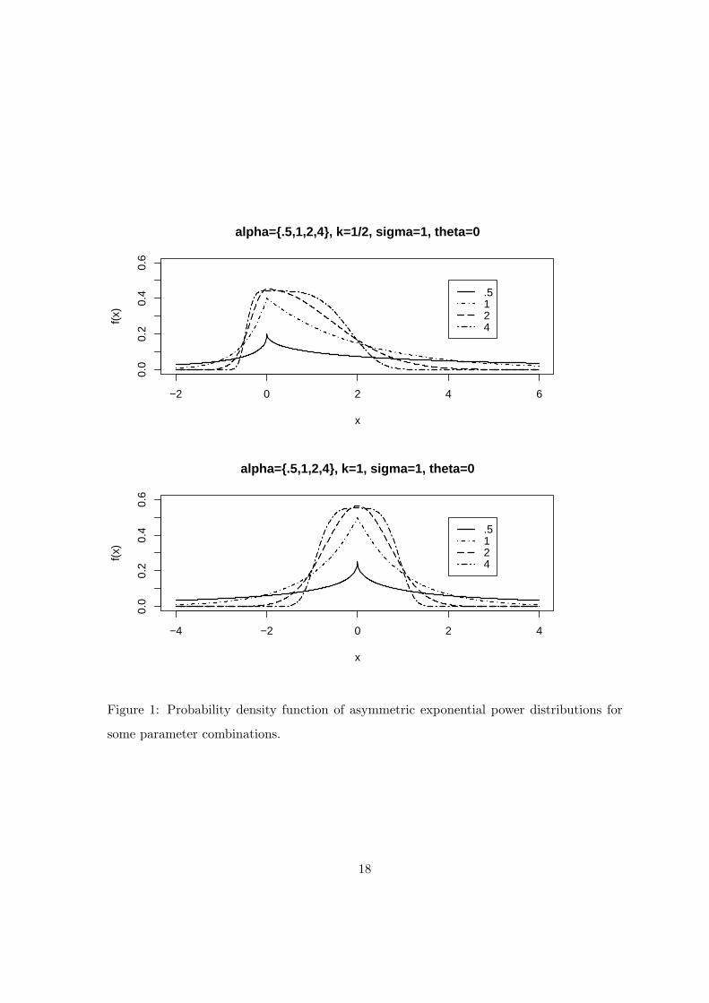
The asymmetric exponential power distribution has the following density function:

f(x) =ακ

σ(1 + κ2)Γ(1/α)exp

{−

(κsgn(x−θ)

( |x− θ|σ

))α},−∞ < x < ∞, (1)

where sgn(u) is the sign of u. Parameters θ and σ > 0 correspond to location and scale

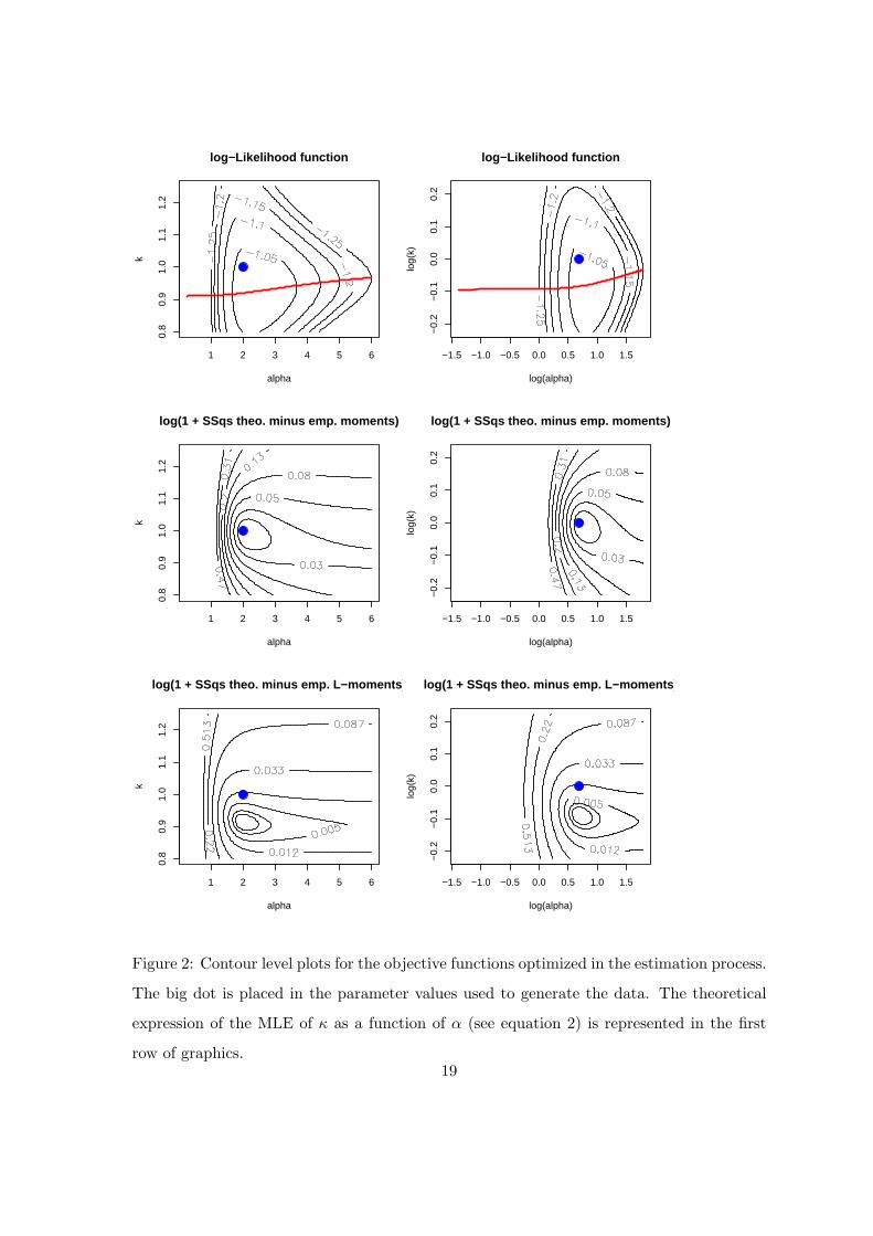
respectively, whereas κ > 0 and α > 0 deal with skewness and shape of distribution. To

have some idea of variety of tail and shape behaviour exhibited by the above model, we give

its graph for some selected value of the parameters in Figure 1.

Ayebo and Kozubowski (2003) follow a general procedure described in Fernandez and

Steel (1998) that allows to introduce a skewed version f of a given symmetric about 0

density function f0:

fk(x) = 2k

1 + k2f0(xκsgn(x)), k > 0.

A different mechanism appears in Azzalini (2005), where the skewed version of f0 is

fAz(x) = 2f0(x)G(w(x)),

where G is the distribution function of an absolutely continuous random variable symmetric

about 0, and w is an odd function. The following result (that can be easily verified)

establishes that under certain conditions the first asymmetrization mechanism is a particular

case of the second one.

Proposition 1 If f0 verifies that limx→∞ f0(δx)/f0(x) = 0 for all δ > 1, then for all x

fk(x) = f∗Az(x) = 2f∗0 (x)G(w(x)), where

f∗0 (x) =k

1 + k2(f0(xk) + f0(x/k)), G(x) =

f0(xksgn(x))f0(xk) + f0(x/k)

, w(x) = sgn(1− k)x.

The condition on the tail behaviour of f0 is needed to show that G is indeed a distribution

function. It is fulfilled when f0 is the exponential power distribution (in this case f0(x) ∝exp(−|x/σ|α)) that is the symmetric density used in equation (1) to define f(x).

The choice of model (1) on the one hand enlarges the previous studies on L-moments

dealing exclusively with extreme values distribution and further allows to verify the claim

by Hosking, Wallis, and Wood (1985) that for models with at least three parameters, the

L-methods fairs better than the other two.

5

To compute the first four L-moments, we need to find

βr =∫

xF (x)rf(x)dx, r = 0, 1, 2, 3,

where F is

F (y) =

κ2

(1+κ2)Γ(1/α, [ (θ−y)

σκ ]α), y < θ

1− 1(1+κ2)Γ(1/α)

Γ(1/α, [κ(y−θ)σ ]α), y ≥ θ,

the distribution function of the asymmetric exponential power random variable, f is its

probability density function and Γ(a, x) is the normalized incomplete Gamma function.

It is not hard to verify the following statements. First, if X has asymmetric exponential

power distribution with parameters θ = (0, σ, κ, α), then −X has also exponential power

distribution with parameters θ = (0, σ, 1/κ, α). Second, if θ = 0, βr(−X) can be obtained

from βr(X) by replacing κ by 1/κ, furthermore

βr(−X) = −∫

x([1− F (x)]rf(x)dx = −αr(X).

Consequently it can be easily verified (see Hosking 1990) that λ3(X) = −λ3(−X) whereas

λ2r(X) = λ2r(−X), r = 1, 2.

This will be used as double check for the computation of L-moments.

Obviously

λ1 = β0 = EX = θ +σ(1/κ− κ)Γ(2/α)

Γ(1/α).

Note that

λr(X) = |b|λr(Y ), X = a + bY,

consequently it is sufficient to find λr/σ, r > 1, from standardized exponential power distri-

bution. By straightforward computation with θ = 0, σ = 1, we find

β1 =∫

xF (x)f(x)dx =κ3(1/κ2 − κ2)Γ(2/α)

(1 + κ2)2Γ(1/α)+

κ2(κ3 + 1/κ3)Γ(2/α)I1/2(1/α, 2/α)(1 + κ2)2Γ(1/α)

,

where I1/2(1/α, 2/α) is normalized incomplete beta function. Hence

λ2 = −σκ(1/κ− κ)2Γ(2/α)(1 + κ2)Γ(1/α)

+ 2σκ2(1/κ3 + κ3)Γ(2/α)I1/2(1/α, 2/α)

(1 + κ2)2Γ(1/α).

6

Next

β2 =κ5(1/κ2 − κ2)Γ(2/α)

(1 + κ2)3Γ(1/α)+ 2

κ4(κ3 + 1/κ3)Γ(2/α)I1/2(1/α, 2/α)(1 + κ2)3Γ(1/α)

+κ3(1/κ4 − κ4)Γ(2/α)∆

(1 + κ2)3Γ(1/α),

where

∆ =1

β(1/α, 2/α)

∫ 1/2

0t(1/α−1)(1− t)(2/α−1)I(1−t)/(2−t)(1/α, 3/α)dt.

Consequently

λ3 =σ(1/κ− κ)(κ4 − 4κ2 + 1)Γ(2/α)

(1 + κ2)2Γ(1/α)

−6σκ3(1/κ− κ)(1/κ3 + κ3)Γ(2/α)I1/2(1/α, 2/α)(1 + κ2)3Γ(1/α)

+6σ(1 + κ4)(1/κ− κ)Γ(2/α)∆

(1 + κ2)2Γ(1/α).

Finally

β3 =κ7(1/κ2 − κ2)Γ(2/α)

(1 + κ2)4Γ(1/α)+

3κ6(1/κ3 + κ3)Γ(2/α)I1/2(1/α, 2/α)(1 + κ2)4Γ(1/α)

+3κ5(1/κ4 − κ4)Γ(2/α)∆

(1 + κ2)4Γ(1/α)+

κ4(κ5 + 1/κ5)Γ(2/α)∆1

(1 + κ2)4Γ(1/α),

where

∆1 =

∫ 1/20

∫ 1−y2−y

0 y(1/α−1)(1− y)(2/α−1)z(1/α−1)(1− z)(3/α−1)I (1−z)(1−y)1+(1−z)(1−y)

(1/α, 4/α)dzdy

β(1/α, 2/α)β(1/α, 3/α)

and

λ4 = −σκ(1/κ− κ)2(κ4 − 8κ2 + 1)Γ(2/α)(1 + κ2)3Γ(1/α)

+12σκ2(κ3 + 1/κ3)(κ4 − 3κ2 + 1)Γ(2/α)I1/2(1/α, 2/α)

(1 + κ2)4Γ(1/α)

−30σκ3(1/κ− κ)2(1/κ2 + κ2)Γ(2/α)∆

(1 + κ2)3Γ(1/α)+ 20

σκ4(1/κ5 + κ5)Γ(2/α)∆1

(1 + κ2)4Γ(1/α).

For symmetric exponential power distribution, i.e., κ = 1, we have λ1 = θ, λ3 = 0 and

also the expressions for λ2, λ4 considerably simplify.

7

4 Simulation study

We have developed a simulation study in order to gain an insight into the performance on

small samples of the three estimation methods: maximum likelihood estimation (MLE),

the moments method (MOM), and the L-moments method (LMO). Two main scenarios are

examined: in the first one the location parameter θ is taken as known (results in Table 1)

whereas in the second case all four parameters are assumed to be unknown (results are in

Table 2).

The log-likelihood function is

log L(α, κ, σ, θ) = n

(log

α

Γ(1/α)+ log

κ

1 + κ2− log σ − κα

σαx+

α −1

κασαx−α

),

where

x+α =

1n

n∑

i=1

([xi − θ]+)α, x−α =1n

n∑

i=1

([xi − θ]−)α,

and [x]+ = max{x, 0}, [x]− = max{−x, 0}.The formulas for computing the MLE of κ and σ (depending on α and θ) are taken from

Ayebo and Kozubowski (2003):

κ = κ(α, θ) =

[x−αx+

α

] 12(α+1)

, (2)

σ = σ(α, θ) =[α(x+

α x−α )α

2(α+1)

([x+

α ]1

α+1 + [x−α ]1

α+1

)] 1α

.

The function of α

log L(α, κ(α, θ), σ(α, θ), θ)

has to be numerically maximized to determine the MLE of α. The value θ is consider to be

known here.

When location parameter has to be estimated (second scenario) we follows the indi-

cation of Ayebo and Kozubowski (2003) and use a non-parametric mode estimator: the

half-range mode estimation method (Bickel 2002). Let θ be this estimator of θ. θ is re-

placed by θ in the expression of x+α and x−α to obtain the corresponding log likelihood

function log L(α, κ(α, θ), σ(α, θ), θ) that is maximized in α. An alternative method should

be to estimate α and θ simultaneously by MLE, maximizing log L(α, κ(α, θ), σ(α, θ), θ) in

8

both parameters. A numerical optimization in two variables should be conducted, and it

would however be hard to distinguish between numerical and statistical performance of the

estimation method. So we decide not to explore this way and follow Ayebo and Kozubowski

(2003) advice.

For the moments method estimation we equate the empirical mean, variance and asym-

metry coefficient to their theoretical counterpart and solve numerically the nonlinear system.

We use the expressions given in Ayebo and Kozubowski (2003):

µ = E(X) = θ + σ

(1κ− κ

)Γ(2/α)Γ(1/α)

,

σ2 = V ar(X) = σ2 Γ(3/α)Γ(1/α)

1 + κ6

κ2(1 + κ2)− σ2 Γ2(2/α)

Γ2(1/α)(1− κ2)2

κ2,

γ = E

[(X − µ

σ

)3]

=

(1− κ8)Γ2( 1α)Γ( 4

α)− 3(1− κ2)(1 + κ6)Γ( 1α)Γ( 2

α)Γ( 3α) + 2(1− κ2)3(1 + κ2)Γ3( 2

α)

(1 + κ2)(Γ(1/α)Γ(3/α)1+κ6

1+κ2 − Γ2(2/α)(1− κ2)2)3/2

.

Observe that only three theoretical moments are needed because, when it is necessary,

parameter θ is estimated by the half-range mode method.

Estimation by the method of L-moments follows a similar mechanics: we look for the

combinations of parameters α, κ, and σ solving the system of equations

λr = lr, r = 1, 2, 3,

where λr are the theoretical L-moments (depending on parameters as it is stated in Section

3) and lr are the empirical L-moments (computed as indicated in Section 2).

We have simulated samples of three different sizes (n = 10, 20, 50). Only a value for

the location parameter (θ = 0) and for the scale parameter (σ = 1) are used because the

use of different location and/or scale values has no effect on the results. Four values for α

(0.5, 1, 2, 4) and two for κ (1/2, 1) are considered. In this way we contemplated the double

exponential case (α = 1, κ = 1), the normal case (α = 2, κ = 1), a more concentrated

symmetric case (α = 4, κ = 1), a very heavy tail symmetric distribution (α = 0.5, κ = 1),

and their right asymmetric versions (κ < 1). The case κ is essentially equivalent to the case

1/κ (only asymmetry direction changes), so we have only considered κ ≤ 1. The number

9

of simulated samples for each combination was S = 5000. Figure 1 shows the theoretical

density functions for the simulated data.

(Figure 1 about here)

All the computations have been done in R (R Development Core Team 2005). In the

MLE of α the one dimensional optimization were carried out with the R-function optimize,

that uses a combination of golden section search and successive parabolic interpolation. For

moments and L-moments estimation, the sum of squares of the differences between empiri-

cal and theoretical moments (or L-moments), as a functions of the unkown parameters, have

been numerically minimized. The parameter combination where the minimum is achieved

is considered as moments (or L-moments) estimator of the unknown parameters. The mul-

tivariate optimization R-function optim was used to minimize these sum of squares. A

quasi-Newton method which allows box constraints (each variable can be given a lower

and/or upper bound) has been chosen. For numerical stability reasons the objective func-

tions were actually the logarithm of 1 plus the sum of squares, expressed as function of

the logs of the parameters α, κ, and σ. All the numerical optimizations have been done

restricting α to the interval [.25, 6], κ to [0.1, 1.2], and σ to [0.5, 2].

Figure 2 shows the contour plots for the objective functions optimized to obtain the

three type of estimators. The sample used to compute these functions has size n = 20 and

was generated with α = 2, κ = 1, σ = 1, and θ = 0. The graphics in the left column use

parameters as optimization variables, and logs of parameters are used in the right column.

It can be seen that the contour level sets are more rounded when parameters are taken in

logs. This fact helps in the numerical optimization process.

(Figure 2 about here)

Tables 1 and 2 show the results of the simulation. The first one corresponds to the case

where θ is assumed to be known, and the second one to scenario with unknown θ. For each

combination of n, α and κ, for each estimation method, and for each estimated parameter

two numbers are displayed: the average over the S = 5000 simulations, and the squared

root of the mean squared error (in brackets and in italic). The figures corresponding to θ

in Table 2 show the performance of the nonparametric estimation of θ.

(Table 1 about here)

10

(Table 2 about here)

We first briefly examine the estimation bias and then we deal with MSE in more detail.

All three methods provide estimates with low bias for σ and large for α and for κ, this one

specifically for asymmetric distributions. On the basis of absolute value of bias estimates,

we see that L-method fairs better than others for shape parameter α whereas for estimating

σ and κ, MLE and moments method share the lead. Obviously size of estimate bias reduces

with increase of n.

A first attempt to analyze the squared root of MSE data could be to fit multifactorial

ANOVA models. Six different models could be fitted, corresponding to the three estimated

parameters (α, σ, κ) and the two scenarios (known or estimated θ). Each ANOVA model

would include the four factors considered in the simulation (see factors and levels listed

bellow) and perhaps second order interactions. Nevertheless our simulation data do not

verify the required hypothesis fot fitting such multifactorial ANOVA models: in fact we are

dealing with a balanced design with only three true factors (n, α and κ) and the response

variable is three dimensional, because for each combination of those factors we observe the

three values of square root of MSE (computed from the same set of S = 5000 simulated

samples) corresponding to the three types of estimator we are comparing. So the specific

estimator in use is not a factor design. Given that strictly speaking it is not possible to fit

univariate multifactorial ANOVA models to the squared root of MSE data, we opted for

doing a descriptive analysis of the data, according to the following factorial structure:

Factor Levels Values

Estimator 3 LMO; MLE; MOM

n 3 10; 20; 50

α 4 0,5; 1,0; 2,0; 4,0

κ 2 0,5; 1,0

Figure 3 shows the main effects plots corresponding to the levels of the above four

factors. Their six panels are a graphical summary of the squared root of MSE values for

Tables 1 (known θ, left column panels) and 2 (estimated θ, right column panels). Each point

represents the mean of all the square root of MSE values corresponding to a combination

of a factor value and an estimated parameter. The interaction between factors are well

summarized by the interaction plots shown in Figures 4, 5, and 6. Here each point is the

11

mean of all the square root of MSE values corresponding to a combination of values for two

factors and an estimated parameter.

(Figure 3 about here)

(Figure 4 about here)

(Figure 5 about here)

(Figure 6 about here)

The following conclusions are derived from the simulation results and the main effects

and interaction plots. We start with the estimation of α in the known θ case (see the first

row first column panel in Figure 3 and the top panel in Figure 4). L-moments method is

recomended for the estimation of α, mainly when n is small (10 or 20), and the true density

has high tails (α small) or is asymmetric (κ = 0.5). When n grows, the MSE of α estimators

decreases, and this happens much more quickly for MLE than for moments or L-moments

estimators. It can be seen that the MSE of α estimators increases when the true α increases.

This is because when the target parameter α is bigger the variability of the estimation is

also bigger. Nevertheless, observe that the MSE corresponding to α = 4 is lower than

that corresponding to α = 2: the more regular shape of the density function when α = 4

compensates the increment of MSE due to the increment in α. The case corresponding to

the estimation of α and unknown θ (estimated by mode estimation) is very similar to the

previous one (see the first row second column panel in Figure 3 and the bottom panel in

Figure 4). The precision in the estimation of α is similar for known or estimated θ, as the

main effects plots show.

Let us go now to the estimation of σ in the known θ case (see the second row first column

panel in Figure 3 and the top panel in Figure 5). In this case the moments estimator is the

recommended one, due mainly to cases α < 2 (heavy tail), κ = 0.5 (asymmetry) and n = 10.

In other cases the MLE is the best one. The L-moments estimator is not recommended

for the estimation of σ. The asymmetric case (κ = .5) brings better estimations of σ than

the symmetric one (κ = 1). When θ is unknown (see the second row second column panel

in Figure 3 and the bottom panel in Figure 5) the MLE is the recommended one. In this

situation is the value of α what mainly determines the performance of the estimators (MSE

values decrease with α). Another noteworthy difference with the known θ case is that now

12

the quality of the estimations does not depend on κ (MSE values are practically constant

in κ). The main effects plots show that σ is much better estimated when θ is known (see

the ordinate scale of the second row of panels in Figure 3).

Finally we deal with the estimation of parameter κ, starting with the known θ case

(see the third row first column panel in Figure 3 and the top panel in Figure 6). Here the

recommended estimator is the one based in L-moments. It is comparable to MLE in the

asymmetric case (κ = 0.5) and clearly better in the symmetric case (κ = 1). A general

fact is that MSE in the estimation of κ is bigger for κ = 1 than for κ = .5. This happens

again (as in estimation of α) because usually the bigger is the parameter the bigger is the

estimators variability. These differences are more remarkable for MLE than for the other

two estimation methods. The corresponding case when θ is unknown (see the third row

second column panel in Figure 3 and the bottom panel in Figure 6) presents a notable

difference with respect to the previous situation: now the MSE increases in α and decreases

in κ, while the opposite happens in the known θ case. Now MLE and L-moments estimator

perform very similarly and both beat the moments estimator. The main effects plots show

that σ is much better estimated when θ is known (see the ordinate scale of the third row of

panels in Figure 3).

As a summary we can say that L-moments method performs well when estimating α or

κ. That is more clear for n = 10 and n = 20, specially for heavy tails densities (α ≤ 1).

MLE is preferable for n = 50. Moreover moments estimator is competitive for small n

and big α. According to the stability to the changes of levels of n and α, the L-moments,

moments and MLE methods can be rated in this order.

From our study on relative performance of the three different estimation methods in

small samples it is clear that no golden rule can be ascribed as to the best one for all

parameters in small samples. Note that this in no way contradicts Hosking and Wallis

(1987) conclusion that L-method outperforms others, as the performance of this estimator

is heavily model dependent in such a situation.

13

5 Conclusions

This article presents the analytical expression of the first four L-moments of the asymmet-

ric exponential power distributions, making possible considering L-method estimators for

the parameters of this distributions family, as an alternative to maximum likelihood and

moments estimation. An extensive simulation study has been developed to compare these

three estimation methods. It shows that the L-moments method is competitive for small

sample sizes and heavy tails distributions.

References

Ayebo, A. and T. J. Kozubowski (2003). An asymmetric generalization of gaussian and

laplace laws. Journal of Probability and Statistical Science 1 (2), 187–210.

Azzalini, A. (1985). A class of distributions which includes the normal ones. Scandinavian

Journal of Statistics 12, 171–178.

Azzalini, A. (2005). The skew-normal distribution and related multivariate families. Scan-

dinavian Journal of Statistics 32, 159–188.

Bickel, D. R. (2002). Robust estimators of the mode and skewness of continuous data.

Computational Statistics and Data Analysis 39 (2), 153–163.

Chan, L. K. (1967). On a characterization of distributions by expected values of extreme

order statistics. Amer. Math. Monthly 74, 950–951.

Fernandez, C. and M. F. J. Steel (1998). On Bayesian modeling of fat tails and skewness.

Journal of the American Statistical Association 93, 359–371.

Greenwood, J. A., J. M. Landwehr, N. C. Matala, and J. R. Wallis (1979). Probability

weighted moments: Definition and relation to parameters of several distributions

expressable in the inverse form. Watwer Resources Research 15 (5), 1049–1054.

Hannan, E. J. (1987). The Cochrane and Orcutt papers. In Specification analysis in the

linear model, Internat. Lib. Econom., pp. 9–18. London: Routledge & Kegan Paul.

Hosking, J. R. M. (1986). The theory of probability weighted moments. Research Report

RC12210, IBM Research, Yorktown Heights.

14

Hosking, J. R. M. (1990). L-moments: Analysis and estimation of distributions using

linear combinations of order statistics. Journal of the Royal Statistical Society, Series

B, Methodological 52, 105–124.

Hosking, J. R. M. and J. R. Wallis (1987). Parameter and quantile estimation for the

generalized Pareto distribution. Technometrics 29 (3), 339–349.

Hosking, J. R. M., J. R. Wallis, and E. F. Wood (1985). Estimation of the generalized

extreme-value distribution by the method of probability-weighted moments. Techno-

metrics 27 (3), 251–261.

Kirby, D. (1974). Algebraic boundedness of sample statistics. Watwer Resources Re-

search 10, 220–222.

Kotz, S., T. J. Kozubowski, and K. Podgorski (2001). The Laplace distribution and gen-

eralizations: a revisit with applications to communications, economics, engineering,

and finance. Birkhuser Verlag.

Mudholkar, G. S. and A. D. Hutson (1998). LQ-moments: Analogs of L-moments. Journal

of Statistical Planning and Inference 71, 191–208.

Mudholkar, G. S. and A. D. Hutson (2000). The epsilon-skew-normal distribution for

analyzing near-normal data. Journal of Statistical Planning and Inference 83 (2), 291–

309.

R Development Core Team (2005). R: A language and environment for statistical comput-

ing. Vienna, Austria: R Foundation for Statistical Computing. ISBN 3-900051-07-0.

Sillitto, G. P. (1969). Derivation of approximants to the inverse distribution function of a

continuous univariate population from the order statistics of a sample. Biometrika 56,

641–650.

Corresponding author: Pedro Delicado, Departament d’Estadıstica i Investigacio Operativa,

Universitat Politecnica de Catalunya, Barcelona, Spain.

E-mail: pedro.delicado@upc.edu

15

n = 10 n = 20 n = 50α κ MLE Mom. L-Mom. MLE Mom. L-Mom. MLE Mom. L-Mom.

0.50 0.50 α 1.58 1.45 0.669 0.763 1.46 0.575 0.556 1.53 0.528(2.13) (2.12) (0.611) (0.776) (2.25) ( 0.3) (0.16) (2.38) (0.101)

σ 0.917 1.08 0.884 0.891 1.06 0.895 0.914 1.03 0.903(0.434) (0.236) (0.354) (0.427) (0.237) (0.345) (0.368) (0.229) (0.332)

κ 0.564 0.637 0.578 0.542 0.632 0.549 0.528 0.624 0.529(0.129) (0.288) (0.175) (0.0822) (0.292) (0.117) (0.0504) (0.288) (0.0624)

1.00 α 1.63 1.03 0.547 0.759 1.07 0.52 0.554 1.08 0.502(2.31) (1.57) (0.309) (0.812) (1.71) (0.215) (0.161) (1.78) (0.143)

σ 0.912 1.07 0.825 0.906 1.05 0.808 0.911 1.03 0.776(0.436) (0.229) (0.384) (0.42) (0.223) (0.389) (0.376) (0.201) ( 0.4)

κ 1.04 0.964 0.982 1.02 0.969 1 1.01 0.969 1(0.331) (0.255) (0.216) (0.209) (0.247) (0.172) (0.121) (0.231) (0.124)

1.00 0.50 α 2.88 2.37 1.74 1.82 1.75 1.35 1.17 1.34 1.11(2.92) ( 2.1) (1.74) (1.73) (1.32) (1.04) (0.502) (0.635) (0.454)

σ 0.924 1.14 0.842 0.939 1.12 0.876 0.969 1.08 0.913(0.369) (0.215) (0.359) (0.335) (0.215) (0.331) (0.256) (0.221) (0.287)

κ 0.549 0.581 0.559 0.537 0.561 0.542 0.522 0.539 0.525(0.104) (0.151) (0.107) (0.0709) (0.113) (0.0729) (0.0413) (0.0712) (0.0435)

1.00 α 3.26 1.65 2.06 1.89 1.32 1.86 1.18 1.05 1.64( 3.3) (1.66) (2.19) (1.84) (1.24) (1.93) (0.503) (0.737) (1.53)

σ 0.958 0.838 0.872 0.972 0.77 0.867 0.98 0.704 0.866(0.359) (0.36) (0.359) (0.312) (0.389) (0.36) (0.252) (0.416) (0.355)

κ 1.04 0.987 0.986 1.01 0.997 0.995 1.01 1.01 1(0.308) (0.183) (0.185) (0.184) (0.153) (0.144) (0.104) (0.118) (0.0976)

2.00 0.50 α 4.22 3.73 3.06 3.65 3.18 2.74 2.62 2.55 2.36(3.07) (2.52) (2.34) (2.56) (2.03) (1.93) (1.37) (1.25) (1.26)

σ 0.871 0.995 0.826 0.94 1 0.878 0.987 1.01 0.946(0.327) (0.237) (0.336) (0.255) (0.207) (0.284) (0.176) (0.169) (0.202)

κ 0.535 0.566 0.556 0.527 0.545 0.538 0.519 0.527 0.523(0.0777) (0.109) (0.0979) (0.0544) (0.0726) (0.0663) (0.0347) (0.0441) (0.0398)

1.00 α 4.84 2.1 4.02 3.71 1.91 3.87 2.63 1.79 3.72(3.45) (1.79) (3.09) (2.59) (1.65) (2.99) (1.39) (1.56) (2.87)

σ 0.932 0.69 0.897 0.985 0.679 0.921 0.998 0.671 0.941(0.284) (0.409) (0.314) (0.223) (0.415) (0.303) (0.167) (0.42) (0.291)

κ 1.03 0.994 0.989 1.01 0.999 0.998 1 1 1(0.259) (0.162) (0.169) (0.159) (0.133) (0.131) (0.0894) (0.095) (0.0881)

4.00 0.50 α 4.93 4.54 3.97 5.11 4.47 4.04 4.77 4.35 4.12(2.06) (1.79) (2.09) (1.83) (1.66) (1.87) (1.52) (1.44) ( 1.6)

σ 0.818 0.938 0.809 0.903 0.963 0.875 0.969 0.982 0.941(0.308) (0.235) (0.324) (0.211) (0.19) (0.252) (0.117) (0.125) (0.153)

κ 0.527 0.565 0.552 0.519 0.541 0.533 0.513 0.524 0.521(0.0595) (0.102) (0.0893) (0.0376) (0.0656) (0.0583) (0.0243) (0.0409) (0.0375)

1.00 α 5.52 2.84 4.65 5.16 2.73 4.68 4.8 2.61 4.64(2.04) (2.44) ( 2.1) (1.87) (2.49) (2.02) (1.54) (2.51) ( 1.8)

σ 0.868 0.711 0.904 0.939 0.701 0.922 0.983 0.693 0.947(0.256) (0.389) (0.272) (0.17) (0.391) (0.237) (0.102) (0.393) (0.193)

κ 1.03 0.999 0.995 1.01 1 1 1 1 1(0.228) (0.153) (0.162) (0.125) (0.12) (0.126) (0.0706) (0.0794) (0.0842)

Table 1: Simulations results. Known θ.

16

n = 10 n = 20 n = 50α κ MLE Mom. L-Mom. MLE Mom. L-Mom. MLE Mom. L-Mom.

0.50 0.50 α 1.3 1.34 0.555 0.672 1.43 0.533 0.518 1.42 0.504(2.08) (2.07) (0.426) (0.857) (2.24) (0.34) (0.159) (2.26) (0.173)

σ 1.11 1.53 1.14 1.1 1.44 1.13 1.11 1.34 1.06(0.695) (0.772) (0.711) (0.669) (0.719) (0.694) (0.617) (0.639) (0.637)

κ 0.65 0.585 0.647 0.608 0.555 0.593 0.567 0.51 0.547( 0.3) (0.389) ( 0.3) (0.218) (0.373) (0.229) (0.137) (0.35) (0.126)

θ 2.1 1.33 0.767( 4) (2.48) (1.38)

1.00 α 1.2 0.998 0.559 0.616 1.04 0.532 0.509 1.06 0.512(1.94) (1.51) (0.312) (0.736) (1.67) (0.219) (0.163) (1.76) (0.123)

σ 1.06 1.53 1.22 1.01 1.41 1.18 1.05 1.28 1.13(0.676) (0.763) (0.75) (0.639) (0.683) (0.738) (0.588) (0.582) (0.719)

κ 0.959 0.909 0.969 0.984 0.917 0.987 0.995 0.92 0.997(0.245) (0.37) (0.246) (0.184) (0.355) (0.19) (0.134) (0.346) (0.137)

θ -0.0188 -0.000895 0.00211(2.25) (1.32) (0.747)

1.00 0.50 α 2.44 1.74 1.38 1.69 1.42 1.16 1.12 1.15 0.962(2.86) (1.51) (1.43) (1.86) (1.06) (1.01) (0.548) (0.522) (0.58)

σ 1.03 1.53 1.05 1.09 1.4 0.995 1.12 1.24 0.891(0.618) (0.755) (0.633) (0.596) (0.685) (0.585) (0.484) (0.557) (0.477)

κ 0.682 0.727 0.71 0.653 0.676 0.665 0.613 0.628 0.615(0.341) (0.325) (0.324) (0.275) (0.257) (0.269) (0.19) (0.184) (0.192)

θ 0.656 0.52 0.373(1.08) (0.844) (0.588)

1.00 α 2.5 1.77 1.96 1.63 1.52 2.03 1.09 1.25 2(2.92) (1.71) (2.02) (1.78) (1.46) (1.99) (0.509) (1.01) (1.82)

σ 0.971 1.12 1.24 1 1.04 1.34 0.981 0.97 1.41(0.584) ( 0.6) (0.694) (0.542) (0.597) (0.737) (0.398) (0.596) (0.764)

κ 0.942 0.968 0.961 0.976 0.983 0.98 0.996 0.996 0.996(0.269) (0.227) (0.235) (0.204) (0.191) (0.195) (0.151) (0.15) (0.148)

θ 0.000593 -0.0086 0.00371(0.62) (0.472) (0.326)

2.00 0.50 α 3.66 2.83 2.55 3.37 2.54 2.46 2.61 2.03 2.13(3.04) (2.03) (2.12) (2.58) (1.85) (2.01) (1.54) (1.33) (1.67)

σ 0.912 1.12 1.03 1.05 1.06 1.01 1.13 0.976 0.964(0.453) (0.463) (0.551) (0.42) (0.417) (0.508) (0.333) (0.359) (0.433)

κ 0.757 0.8 0.812 0.734 0.758 0.779 0.695 0.705 0.732(0.415) (0.395) (0.411) (0.361) (0.346) (0.379) (0.291) (0.282) (0.327)

θ 0.565 0.503 0.408(0.833) (0.73) (0.587)

1.00 α 3.76 2.58 3.64 3.38 2.68 3.98 2.5 2.83 4.26(3.09) (1.93) (2.77) (2.58) (2.03) (2.95) ( 1.4) (2.17) (3.07)

σ 0.792 0.836 1.02 0.895 0.855 1.06 0.951 0.88 1.1(0.391) (0.388) (0.472) (0.324) (0.362) (0.413) (0.221) (0.343) (0.345)

κ 0.93 0.957 0.955 0.96 0.971 0.964 0.986 0.985 0.982( 0.3) (0.247) (0.249) (0.241) (0.223) (0.231) (0.19) (0.188) (0.199)

θ -0.000172 -0.000527 0.00682(0.464) ( 0.4) (0.322)

4.00 0.50 α 4.35 3.21 3.39 4.72 3.42 3.55 4.64 3.58 3.65( 2.4) (2.07) (2.24) (2.02) (1.98) (2.13) (1.63) ( 1.9) (1.97)

σ 0.829 1 1.05 0.99 1.03 1.07 1.1 1.04 1.08(0.364) (0.369) (0.495) (0.29) (0.336) (0.442) (0.237) (0.312) (0.389)

κ 0.82 0.871 0.876 0.801 0.835 0.844 0.787 0.809 0.821(0.473) (0.461) (0.469) (0.438) (0.432) (0.445) (0.403) (0.408) (0.424)

θ 0.618 0.558 0.513(0.857) (0.78) (0.711)

1.00 α 4.47 3.19 3.98 4.77 3.44 4.32 4.65 3.91 4.72(2.39) (2.09) (2.11) (2.02) (2.02) (2.01) (1.61) ( 1.9) (1.87)

σ 0.706 0.803 0.935 0.814 0.829 0.969 0.906 0.885 1.01(0.364) (0.326) ( 0.4) (0.272) (0.286) (0.35) (0.162) (0.226) (0.277)

κ 0.905 0.944 0.941 0.94 0.955 0.951 0.959 0.96 0.954(0.335) (0.269) (0.271) (0.284) (0.256) (0.262) (0.242) (0.24) (0.248)

θ 0.0014 0.0119 0.0038(0.461) (0.426) (0.38)

Table 2: Simulations results. Unknown θ.

17

−2 0 2 4 6

0.0

0.2

0.4

0.6

alpha={.5,1,2,4}, k=1/2, sigma=1, theta=0

x

f(x)

.5124

−4 −2 0 2 4

0.0

0.2

0.4

0.6

alpha={.5,1,2,4}, k=1, sigma=1, theta=0

x

f(x)

.5124

Figure 1: Probability density function of asymmetric exponential power distributions for

some parameter combinations.

18

log−Likelihood function

alpha

k

1 2 3 4 5 6

0.8

0.9

1.0

1.1

1.2

log−Likelihood function

log(alpha)

log(

k)

−1.5 −1.0 −0.5 0.0 0.5 1.0 1.5

−0.

2−

0.1

0.0

0.1

0.2

log(1 + SSqs theo. minus emp. moments)

alpha

k

1 2 3 4 5 6

0.8

0.9

1.0

1.1

1.2

log(1 + SSqs theo. minus emp. moments)

log(alpha)

log(

k)

−1.5 −1.0 −0.5 0.0 0.5 1.0 1.5

−0.

2−

0.1

0.0

0.1

0.2

log(1 + SSqs theo. minus emp. L−moments)

alpha

k

1 2 3 4 5 6

0.8

0.9

1.0

1.1

1.2

log(1 + SSqs theo. minus emp. L−moments)

log(alpha)

log(

k)

−1.5 −1.0 −0.5 0.0 0.5 1.0 1.5

−0.

2−

0.1

0.0

0.1

0.2

Figure 2: Contour level plots for the objective functions optimized in the estimation process.

The big dot is placed in the parameter values used to generate the data. The theoretical

expression of the MLE of κ as a function of α (see equation 2) is represented in the first

row of graphics.19

Me

an

of

MS

E

MOMMLELMO

2,0

1,5

1,0

502010

4,02,01,00,5

2,0

1,5

1,0

1,00,5

Estimato n

alpha k

Main Effects Plot for MSE estimating alpha

Me

an

of

MS

E

MOMMLELMO

2,0

1,5

1,0

502010

4,02,01,00,5

2,0

1,5

1,0

1,00,5

Estimato n

alpha k

Main Effects Plot for MSE estimating alpha

Me

an

of

MS

E

MOMMLELMO

0,325

0,300

0,275

0,250

502010

4,02,01,00,5

0,325

0,300

0,275

0,250

1,00,5

Estimato n

alpha k

Main Effects Plot for MSE estimating sigma

Me

an

of

MS

E

MOMMLELMO

0,7

0,6

0,5

0,4

0,3

502010

4,02,01,00,5

0,7

0,6

0,5

0,4

0,3

1,00,5

Estimato n

alpha k

Main Effects Plot for MSE estimating sigma

Me

an

of

MS

E

MOMMLELMO

0,18

0,16

0,14

0,12

0,10

502010

4,02,01,00,5

0,18

0,16

0,14

0,12

0,10

1,00,5

Estimato n

alpha k

Main Effects Plot for MSE estimating k

Me

an

of

MS

E

MOMMLELMO

0,36

0,33

0,30

0,27

0,24

502010

4,02,01,00,5

0,36

0,33

0,30

0,27

0,24

1,00,5

Estimato n

alpha k

Main Effects Plot for MSE estimating k

Figure 3: Main effects plots for the square root of MSE values from Tables 1 (known θ,

left column) and 2 (estimated θ, right column). First row of graphics represents the square

root of MSE in the estimation of α, second row corresponds to the estimation of σ, and the

third one to the estimation of κ.

20

Estimato

502010 4,02,01,00,5 1,00,5

2

1

0

n

2

1

0

alpha

2

1

0

k

Estimato

MOM

LMO

MLE

n

50

10

20

alpha

2,0

4,0

0,5

1,0

Interaction Plot (data means) for MSE

Estimato

502010 4,02,01,00,5 1,00,5

2

1

0

n

2

1

0

alpha

2

1

0

k

Estimato

MOM

LMO

MLE

n

50

10

20

alpha

2,0

4,0

0,5

1,0

Interaction Plot (data means) for MSE

Figure 4: Estimation of α. Interaction plot for the MSE values. Top panel: known θ.

Bottom panel: estimated θ.21

Estimato

502010 4,02,01,00,5 1,00,5

0,4

0,3

0,2

n

0,4

0,3

0,2

alpha

0,4

0,3

0,2

k

Estimato

MOM

LMO

MLE

n

50

10

20

alpha

2,0

4,0

0,5

1,0

Interaction Plot (data means) for MSE

Estimato

502010 4,02,01,00,5 1,00,5

0,6

0,4

0,2

n

0,6

0,4

0,2

alpha

0,6

0,4

0,2

k

Estimato

MOM

LMO

MLE

n

50

10

20

alpha

2,0

4,0

0,5

1,0

Interaction Plot (data means) for MSE

Figure 5: Estimation of σ. Interaction plot for the MSE values. Top panel: known θ.

Bottom panel: estimated θ.22

Estimato

502010 4,02,01,00,5 1,00,5

0,24

0,16

0,08

n

0,24

0,16

0,08

alpha

0,24

0,16

0,08

k

Estimato

MOM

LMO

MLE

n

50

10

20

alpha

2,0

4,0

0,5

1,0

Interaction Plot (data means) for MSE

Estimato

502010 4,02,01,00,5 1,00,5

0,4

0,3

0,2

n

0,4

0,3

0,2

alpha

0,4

0,3

0,2

k

Estimato

MOM

LMO

MLE

n

50

10

20

alpha

2,0

4,0

0,5

1,0

Interaction Plot (data means) for MSE

Figure 6: Estimation of κ. Interaction plot for the MSE values. Top panel: known θ.

Bottom panel: estimated θ.23