the circumcircles of all the triangles in the net are empty. This definition can be185
extended to 3-D domains by using a circumscribed sphere in place of the circum-186
circle.
Figure 1: Illustration of barycentric co-ordinates of x with respect to a triangle v0,v1, v2; they are the ratios between the areas of the separate sub-triangles to the areaof the entire triangle
187
DMS-splines (also called as triangular B-spline), developed by Dahmen, Micchelli188
and Seidel (1992), are essentially weighted sums of simplex splines. They combine189
the overall global smoothness of simplex splines with the local control properties190
of B-patches (Franssen 1995). For completeness and a ready reference, DMS-191
splines in 2-D are briefly touched upon. Also outlined are the method of generating192
knotclouds and evaluation procedures of simplex and DMS-splines.193
The jth barycentric co-ordinate of a point x in R2, with respect to a triangle withvertices, v0, v1 and v2 for 0 j 2 is given by:
λ j (xjv0v1v2) =Vol ((v0v1v2)(v j:=x))
Vol (v0v1v2)(1a)
Thus one may write
x =Z 2
j=0λ j (xjv0v1v2)v j (1b)
The half-open convex hull of a triangle V , denoted as [V ), is a subset of the convex194
hull of a triangle, such that for every point x in a triangulation one can determine195
exactly one triangle to which x belongs. Thus, for x lying on an edge shared by two196
triangles, it still only belongs to only one of the half-open convex hulls of those197
triangles. But, if x lies on the boundary of the discretized domain, it might not198
CMES Galley Proof Only Please Return in 48 Hours.
Proo
f
A Smooth Finite Element Method 7
belong to any triangle, although it does belong to the convex hull of the polygon.199
An exposition on how to arrive at the half-open convex hull of a triangle is available200
in Franssen (1995).201
2.1 Simplex Splines202
The simplex spline is a multivariate generalization of the well-known univariate203
B-splines. A degree n simplex spline is a smooth, degree n piecewise polynomial204
function defined over a set of n+Ndim +1 points x 2RNdim called knots and the set205
of knots, knotset. If the knotset does not contain a collinear subset of (3 or more)206
knots then the simplex spline has overall Cn1 continuity. A detailed discussion of207
the theory of simplex splines is available in Micchelli (1995). We presently focus208
on bivariate simplex splines. A simplex spline defined over a knotset V is denoted209
as M (:jV ) and its value at x 2 R2 is denoted as M (xjV ).210
A constant simplex spline, defined over 3 knots and knotset V = fv0;v1;v2g, isgiven by:
M (xjV ) =
(1
jdet(V )j if x 2 [V )
0 if x =2 [V )(2)
A higher order simplex spline of degree n with knotset V is defined recursively as aweighted sum of three simplex splines, each of degree n1. The number of verticesof the polygon over which nth degree simplex spline is defined is m = n+2+1. Sothe cardinality of V is n+3. The knotsets for the three n1 degree simplex splinesare chosen from V , leaving out one of the selected knots from V at a time as shownin Fig.2 in which the construction of a quadratic simplex spline is explained. Theselected knots are marked by double circles. The support of the simplex spline isthe half-open convex hull of V . The quadratic simplex spline is a weighted sum ofthree linear simplex splines, the domains of which are shown in Fig.2. Barycentricco-ordinates of x with respect to the selected triangle formed by the circled knotsare used as the weights for the degree n 1 simplex splines when evaluated at x.The recursive formula for the evaluation of degree n simplex splines is thus givenby:
M (xjV ) =Z 2
j=0λ j (xjW )M
xjVn
w j
(3)
where W = fw0;w1;w2g V is the selected (non-degenerate) triangle. Any such211
W from the knotset V is sufficient to generate the simplex spline of degree n at212
x. While the constant simplex spline is discontinuous at its domain boundary, the213
linear simplex spline is C0 and the degree-n simplex spline is Cn1 everywhere214
Figure 2: Selection of knotsets for 3 linear simplex splines to generate a quadraticsimplex spline as their weighted sum: out of the three knots selected, one is leftout, respectively, to form knotsets for the linear simplex splines
2.2 DMS-splines in R2216
DMS-splines, which are weighted sum of simplex splines, are functions that com-217
bine the global smoothness of simplex splines with the desirable local control fea-218
ture of B-patches (see Franssen 1995 for a detailed exposition). The domain of a219
DMS-spline surface is a proper triangulation I R2. In every vertex vi, a knot-220
cloud of n+1 knots, denoted as fvi0; : : : ;ving with vi0 = vi, is defined. The knotsets221
are defined from these knotclouds. A set of control points inR3 are defined for each222
triangle I 2I for a degree n surface. The control points are denoted as cIβ
where223
β is a triple (β0;β1;β2) with jβ j= β0 +β1 +β2 = n. There are exactly (n+1)(n+2)2224
such β . The projections of the control points from R3 to R2 serve as particles in the225
generation of shape functions. A triangular domain, knotclouds and projection of226
control points on R2 (cIβ) for constructing a quadratic DMS-spline in 2D is shown227
in Fig.3. The closer cIβ
lies to a vertex v j of I, the more knots are taken from the228
corresponding knotcloud to form the knotset in the construction of simplex splines.229
Let VIβ=n
vI0β0
;vI1β1
;vI2β2
obe a triangle consisting of the last knots of the heads
of knotclouds in VIβ
. The constant multiplier of M:jVI
β
in the calculation of a
DMS-spline isdet
V I
β
. The DMS-spline basis functions at x corresponding to
CMES Galley Proof Only Please Return in 48 Hours.
Proo
f
A Smooth Finite Element Method 9
Let V , , be a triangle consisting of the last knots of the heads of
knotclouds in V . The constant multiplier of . |V in the calculation of a DMS-spline is
. The DMS-spline basis functions at x corresponding to is |V .
The point on a surface corresponding to is given by
| | |V 4
Fig.3. Parameters for a quadratic DMS-spline: the knotclouds of all vertices are the set , , , , , , , , and are control points; the black circles represent knots and white circles, control points
It is proved (Dahmen et al. 1992) that |V 0 and , | | and ∑ ∑| | |V 1 (partition of unity). A triangle may also have non-
zero contributions to points x in the domain that do not belong to the half-open convex hull of
the triangle. This is a fundamental difference with the usual Bézier patch surface, whose
values can be evaluated for each patch independently. This interference of triangles amongst
themselves establishes the overall global smoothness of DMS-splines. The part of the surface
corresponding to a specific triangle I is a DMS-patch, which is not only the contribution of
this triangle, but the sum of contributions of all triangles to the point .
2.3. Generation of Knotclouds
I
Figure 3: Parameters for a quadratic DMS-spline: the knotclouds of all vertices arethe set V I
β= v(00)
I;v(01)I;v(02)
I;v(10)I;v(11)
I;v(12)I;v(20)
I;v(21)I;v(22)
I and cIβ
are control points; the black circles represent knots and white circles, control points
cIβ
isdet
V I
β
MxjVI
β
. The point on a surface corresponding to x2 R2 is given
by
F (x) =Z
I2I
Zjβ j=n
det
V Iβ
MxjVI
β
cI
β(4)
It is proved (Dahmen et al. 1992) thatdet
V I
β
MxjVI
β
0 8 I 2 I and230
β ; jβ j= n andR
I2I
Rjβ j=n
det
V Iβ
MxjVI
β
= 1 (partition of unity). A triangle231
I 2I may also have non-zero contributions to points x in the domain that do not232
belong to the half-open convex hull of the triangle. This is a fundamental difference233
with the usual Bézier patch surface, whose values can be evaluated for each patch234
independently. This interference of triangles amongst themselves establishes the235
overall global smoothness of DMS-splines. The part of the surface corresponding236
to a specific triangle I is a DMS-patch, which is not only the contribution of this237
triangle, but the sum of contributions of all triangles to the point x 2 I.238
Figure 4: Knot generation in a bracket after triangulation to construct (a) quadraticDMS-splines and (b) cubic DMS-splines
CMES Galley Proof Only Please Return in 48 Hours.
Proo
f
A Smooth Finite Element Method 13
V = fv0;v1; : : : ;vn+1;vn+2g. The recurrence formula is given as Eq. (3). The for-304
mula involves the evaluation of 3n1 linear simplex splines and 3n constant sim-305
plex splines in a naïve approach, as shown in Fig.5. But, by carefully identifying306
the repetitions of simplex splines of various degree, number of evaluations can be307
significantly reduced. The first three knots of knotsets of every simplex spline are308
chosen as the set W (see Eq.3) in a straightforward approach. The number of in-309
dependent linear and constant simplex splines to be evaluated will be n(n+1)2 and310
(n+1)(n+2)2 , respectively (Table 1).
Figure 5: Each node in the tree represents a simplex spline to be evaluated to getthe simplex spline represented by the root node; the number of simplex splines ineach level = kn, where k is the level of evaluation, starting from top
311
2.4.2 Evaluation of DMS-splines312
A degree n DMS-spline basis function, evaluated at a point x 2 R2, is defined313
over the control points cIβ
(Eq. 4) and is given bydet
V I
β
MxjVI
β
, where314
M
xjVIβ
is a simplex splines of degree n and V I
β, a triangle consisting of the315
end knots of the knotclouds of the three vertices of the triangle I, corresponding316
to a control point cIβ
, i.e. V Iβ=n
vI0β0
;vI1β1
;vI2β2
o. The number of control points is317
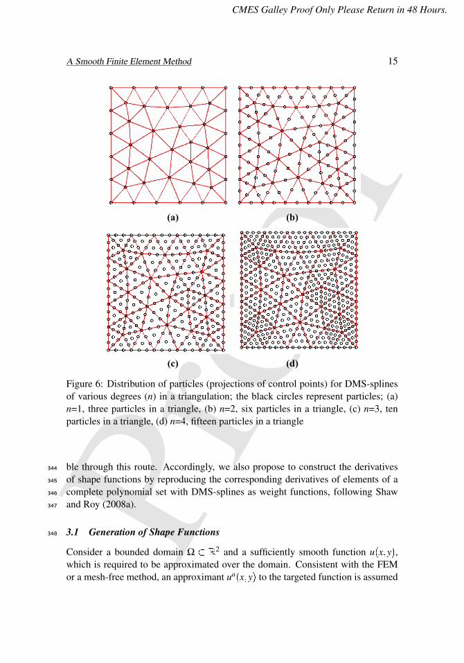
equal to (n+1)(n+2)2 in R2. For each triangle I in I , the particles are located as the318
projections of control points on the triangle, as shown in Figs.6(a) through (d).319
Generation of globally smooth shape functions in 2D domain with DMS-splines321
as weight functions will be discussed in this section. The DMS-spline in R2 is322
denoted as Φ(x;y). A DMS-spline is supported over a triangle and its knotcloud323
neighbourhood defined as the polygon formed by connecting the knots, distributed324
following the restrictions mentioned in Section 2.3 and located close to the vertices325
of the triangle. DMS-spline is constructed corresponding to a given nodal point x in326
a physical domain in R2, over the triangle to the half-open convex hull of which x327
belongs. In general, DMS-splines satisfy the partition of unity and their derivatives328
(including the splines themselves) are globally smooth. But, a direct functional ap-329
proximation based on these functions and their derivatives may sensitively depend330
on the placement of knots around the vertices of triangles. Thus, when the knots are331
far away from or very close to the vertices, the DMS-splines may numerically devi-332
ate from the partition of unity property and the total volume under their derivatives333
may not be close to zero, especially for x close to or on the boundary of the trian-334
gle. So, use of DMS-splines and their derivatives directly as shape functions and335
derivatives of shape functions (respectively) may lead to considerable errors in the336
approximation of a variable (results from a numerical example to illustrate this is337
given in Figs.11 and 12). We propose to study if an explicit reproduction of polyno-338
mials could help overcome this difficulty. Thus the shape functions are constructed339
by the reproduction of all the elements in a complete set of polynomials (a set con-340
taining all the terms in the Pascal’s triangle) of degree p n, with DMS-splines341
as weight functions. It is hoped that a numerical robust imposition of the partition342
of unity property and global smoothness for the shape functions might be possi-343
CMES Galley Proof Only Please Return in 48 Hours.
Proo
f
A Smooth Finite Element Method 15
(d) (c)
(b) (a)
Figure 6: Distribution of particles (projections of control points) for DMS-splinesof various degrees (n) in a triangulation; the black circles represent particles; (a)n=1, three particles in a triangle, (b) n=2, six particles in a triangle, (c) n=3, tenparticles in a triangle, (d) n=4, fifteen particles in a triangle
ble through this route. Accordingly, we also propose to construct the derivatives344
of shape functions by reproducing the corresponding derivatives of elements of a345
complete polynomial set with DMS-splines as weight functions, following Shaw346
and Roy (2008a).347
3.1 Generation of Shape Functions348
Consider a bounded domain Ω R2 and a sufficiently smooth function u(x;y),
which is required to be approximated over the domain. Consistent with the FEMor a mesh-free method, an approximant ua(x;y) to the targeted function is assumed
where Nnd represents the number of nodes in the domain, ui = u(xi;yi) is the valueof the targeted function at particle i and Ψi(x;y) are the globally smooth shapefunctions. Following the practice in many mesh-free methods (e.g. the reproducingkernel methods (Liu, et al. 1995a, Shaw, et al. 2008a, etc), the latter can be writtenas:
Ψi(x;y) = HT (x xi;y yi)b(x;y)Φ(x xi;y yi) (6)
where HT (x;y) is a set of polynomials defined as
xαyβjα+β jp, p is degree of
polynomial (p n), b(x;y) are coefficients of the polynomials in H and Φ(x xi;y yi)is the DMS-spline based at (xi;yi) acting as the weight function. The coefficientsb(x;y) are obtained based on the following polynomial reproduction conditions:
is the so-called moment matrix. So the coefficient vector is given by:
b(x;y) = M1(x;y)H(0)
provided that the moment matrix is invertible. We will be considering this issueshortly. Presently, the global shape functions in two-dimensions are given by:
If a nodal point x is inside a triangle, the support of the shape function is defined349
by a polygon that contains the triangle and is formed by the knotcloud associated350
with the vertices of that triangle as shown in Fig. 7a. If x falls on an edge shared351
by two triangles, the polygonal support of the shape function will include both the352
triangles sharing that edge as shown in Fig. 7b. As a third alternative, if x coincides353
with a common vertex shared by several triangles, then the support for the shape354
function will be in the form of a polygon containing all these triangles which share355
that vertex (Fig. 7c).356
(c) (b) (a)
xx
x
Figure 7: Supports (outer polygons) of shape functions when the nodal point x(red dot) is (a) inside a triangle, (b) on an edge shared by two triangles and (c) onone of the vertices of triangles; the knotcloud shown as black dots is for quadraticDMS-splines
3.2 Derivatives of Shape Functions357
A stable and numerically accurate scheme for computing derivatives of globallysmooth shape functions has been proposed by Shaw and Roy (2008a). It is basedon the premise that γ th derivatives of such shape functions reproduce γ th derivativesof any arbitrary element of the space Pp of polynomials of degree p jγj. Usingthis principle, consistency relations for the derivatives may be written as:Z Nnd
Belytschko 1999). This difficulty is generally overcome via a substantial increase in the order
of quadrature in many mesh-free methods. In the present scheme, the physical domain is
initially represented by a triangulation that enables construction of the DMS-spline basis
functions. Recall from Section 3.1 that the local support of the shape functions is a triangle or
triangles and associated knotcloud neighbourhood. But, since the knot lengths (distance to an
extra knot associated to a vertex from the vertex) are chosen to be very small compared to the
triangle edges, the local support may be considered as the triangle or triangles themselves for
the purpose of numerical integration. So, the triangulation itself serves as integration mesh in
the present scheme. Roughly speaking, a coarse triangulation with higher order quadrature or
a fine triangulation with lower order quadrature should generally give good results. In the
NURBS-based parametric bridge method (Shaw, et al. 2008b), since the mesh in the
parametric space is used as integration cells, the number of such cells will be in excess of
what might have been sufficient. Moreover, the alignment of integration cells and the
supports of shape functions is usually not available for 2. In other methods like the
element free Galerkin (EFG), higher order quadrature is used for more accurate integration.
The present scheme is free of any such misalignment issues because of the uniformity in the
placement of knots and the extra knots being not used as particles (nodes). Numerical
experiments with the present method show that just a 3-point Gauss quadrature with
quadratic DMS-splines (along with a rather fine triangulation; Fig 9a) or a 7-point Gauss
quadrature with cubic or quartic DMS-splines (with a coarse triangulation; Fig 9b and 9c) is
adequate to get good accuracy.
Fig. 8. Misalignment of local support domain (circle) and background integration cells (rectangular) in a mesh-free method (particles are black dots)
Figure 8: Misalignment of local support domain (circle) and background integra-tion cells (rectangular) in a mesh-free method (particles are black dots)
(a) (b) (c)
Figure 9: Aligned local domain (triangles) of DMS-spline basis functions and inte-gration cells (triangles) in the present scheme (particles are red dots); fine to coarsetriangulations
CMES Galley Proof Only Please Return in 48 Hours.
Proo
f
A Smooth Finite Element Method 19
Here bγ(x;y) is the vector of unknown coefficients for derivative reproduction. The
Belytschko 1999). This difficulty is generally overcome via a substantial increase391
in the order of quadrature in many mesh-free methods. In the present scheme, the392
physical domain is initially represented by a triangulation that enables construction393
of the DMS-spline basis functions. Recall from Section 3.1 that the local support394
of the shape functions is a triangle or triangles and associated knotcloud neigh-395
bourhood. But, since the knot lengths (distance to an extra knot associated to a396
vertex from the vertex) are chosen to be very small compared to the triangle edges,397
the local support may be considered as the triangle or triangles themselves for the398
purpose of numerical integration. So, the triangulation itself serves as integration399
mesh in the present scheme. Roughly speaking, a coarse triangulation with higher400
order quadrature or a fine triangulation with lower order quadrature should gener-401
ally give good results. In the NURBS-based parametric bridge method (Shaw, et al.402
2008b), since the mesh in the parametric space is used as integration cells, the num-403
ber of such cells will be in excess of what might have been sufficient. Moreover,404
the alignment of integration cells and the supports of shape functions is usually405
not available for n > 2. In other methods like the element free Galerkin (EFG),406
higher order quadrature is used for more accurate integration. The present scheme407
is free of any such misalignment issues because of the uniformity in the placement408
of knots and the extra knots being not used as particles (nodes). Numerical ex-409
periments with the present method show that just a 3-point Gauss quadrature with410
quadratic DMS-splines (along with a rather fine triangulation; Fig 9a) or a 7-point411
Gauss quadrature with cubic or quartic DMS-splines (with a coarse triangulation;412
Fig 9b and 9c) is adequate to get good accuracy.413
3.5 Imposition of essential boundary conditions414
The shape functions in the present scheme, like many other mesh free shape func-tions, do not satisfy the Kronecker delta property. This makes them non-interpolatingand hence a direct imposition of Dirichlet boundary conditions is not straightfor-ward. Several solutions to this problem have been reported in the literature (Soniaand Antonio 2004, Cai and Zhu 2004, Shuyao and Atluri 2002, Zhu and Atluri1998, etc.). The penalty method is adopted in this work to impose the Dirichlet(essential) boundary conditions. Thus, consider the boundary value problem givenby:
4u = f in Ω
u = ud on Γd;
∇u s = gs on Γs
(15)
where Γd [Γs = ∂Ω and s is the outward normal unit vector on ∂Ω. If the shapefunctions are interpolating (so that the test functions are identically zero on the
CMES Galley Proof Only Please Return in 48 Hours.
Proo
f
A Smooth Finite Element Method 21
Dirichlet boundary) the weak form associated with Eq. (15) is:Z
Ω
∇v ∇udΩZ
Γs
v∇u sdΓ =Z
Ω
v f dΩ (16)
where v and u are the test and trial functions respectively. With the use of thepenalizer α , the weak form can be rewritten as:Z
Ω
∇v ∇udΩZ
Γs
vgsdΓ =Z
Ω
v f dΩ+Z
Γd
α (uud)vdΓ (17)
A proper choice of the penalizer α (usually chosen to be a large positive number)415
should lead to an accurate imposition of the Dirichlet boundary conditions. Indeed,416
as α !∞, one can show that the solution u corresponding to the weak form (17) sat-417
isfies the Dirichlet condition. However, quite unlike the NURBS-based parametric418
bridge method (Shaw et al. 2008b), shape functions (especially those correspond-419
ing to the triangle vertices) via the present scheme are ‘nearly interpolating’. This420
can be observed from the fact that the typical knot-length is presently smaller than421
the characteristic triangle size by at least an order or more. Hence, referring to Fig.422
7(a) for instance, the triangle and the support of the shape function nearly overlap.423
In other words, using the partition of unity property and the fact that shape func-424
tions must be zero on the support boundary, it follows that the shape function for a425
nodal point nearly attains the value of unity at that node (especially if the node is a426
vertex).427
3.6 Sparseness of the stiffness matrix428
The smoothness in the functional approximation in most meshless methods typi-429
cally require that the ‘band’ of interacting nodes is larger than that in the FEM.430
This leads to a larger bandwidth of the stiffness matrix and in turn an increased431
computational time for the inversion of the discretized equations. While the present432
method shares common FE-based domain decomposition (via Delaunay triangula-433
tion), the shape functions are nevertheless generated by the reproducing kernel par-434
ticle technique. In this context, we recall that the compact support of the proposed435
shape function (as well as its derivatives) is nearly the triangle itself (with respect436
to which it is constructed) and that the compact support contains only the minimum437
number of particles required for the inversion of the moment matrix. This observa-438
tion, combined with the adoption of the triangles themselves as background inte-439
gration cells, naturally leads to the computed system stiffness matrix being sparse440
(i.e., with the smallest bandwidth permissible within the polynomial reproducing441
framework) and hence the sparse equation solvers, often used with commercially442
available FEM codes, can be employed in the present method too.443
First, we consider polynomial and non-polynomial (trigonometric and exponential)445
functions, and their derivatives up to fourth order and approximate them over a446
square domain with DMS-spline based global shape functions. The need for poly-447
nomial reproduction in deriving the shape functions is brought forth in the first448
example. Solutions of Laplace’s and Poisson’s equations and comparisons with ex-449
act solutions are presented next. Solutions of a few second order boundary value450
problems, involving plane stress and plane strain cases, are then attempted with451
the present method and comparisons provided with a few other available methods,452
e.g. the parametric mesh-free method, RKPM and FEM with Q4 (4-noded quadri-453
lateral) as well as T6 (6-noded triangle) elements. Problems involving non-simply454
connected domains are also solved to demonstrate the advantages of the present455
method over the NURBS-based parametric bridge method. Ne denotes the number456
of triangles in the triangulation, in the following tables and figures.457
Figure 10: A square domain of dimension 11; the function values and their deriva-tives are calculated at points marked as red dots
CMES Galley Proof Only Please Return in 48 Hours.
Proo
f
A Smooth Finite Element Method 23
Fig.11. Plots of absolute error magnitudes for , at the evaluation points; (a) using standard DMS shape functions; (b) using polynomial reproducing DMS shape
functions and (c) a direct comparison of errors in both cases
Figure 11: Plots of absolute error magnitudes for f (x;y) = x+ y at the evaluationpoints; (a) using standard DMS shape functions; (b) using polynomial reproducingDMS shape functions and (c) a direct comparison of errors in both cases
4.1 Approximating a Few Target Functions and their Derivatives458
4.1.1 Polynomial functions459
In order to illustrate the need for polynomial reproduction whilst generating theshape functions, a linear polynomial function, f (x;y) = x+y and its first derivativewith respect to x are evaluated at 16 points (represented by the red dots in Fig. 10) ina square domain of dimension 11 (unit2) with standard DMS-spline based shapefunctions (without polynomial reproduction) and polynomial reproducing DMS-spline based shape functions. In both cases, linear DMS-splines are used withthe domain being discretized by 16 particles and 18 triangles. The absolute errormagnitudes in both cases vis-à-vis the exact values are plotted against the functionevaluation points in Figs. 11 and 12. Remarkably, large errors in the approximated
The construction of the standard DMS-spline basis functions is done over a triangulated
domain with additional knots in the neighbourhood of the triangle vertices, as explained in
Section 2. For a point x well within the domain (away from the triangle edges), the basis
functions follow partition of unity and total volume under the derivative functions is zero
(modulo very small approximation errors). But when x is close to the triangle edges and the
knots are too close or far away from the vertices, errors creep in computing the basis
functions and their derivatives, which deviate from the above properties. This high sensitivity
of the basis functions to the knot placement is consistently observed across the numerical
experiments. Shape functions via polynomial reproduction are thus consistently adopted to
overcome this difficulty.
Table 2. Relative error norms of polynomial functions and their derivatives with non-polynomial reproducing (standard) DMS-spline shape functions
Fig.12. Plot of absolute errors in the first derivative of function , against the points at which the function is evaluated, (a) using non-polynomial reproducing shape functions (b)
using polynomial reproducing shape functions and (c) comparison of errors in both cases
Figure 12: Plot of absolute errors in the first derivative of function f (x;y) = x+ yagainst the points at which the function is evaluated, (a) using non-polynomialreproducing shape functions (b) using polynomial reproducing shape functions and(c) comparison of errors in both cases
function and its derivative are observed if the explicit condition of polynomial re-production is dropped in the derivation of the shape functions. Moreover, it is alsoobserved from Table 2 that, while an increase in the degree of DMS-splines doesnot decrease the error substantially, an increase in the number of triangles reducesthe error, to an extent, in the case of standard DMS shape functions. Similar re-sults, shown in Table 3 through the polynomial reproducing shape functions, areonce more indicative of the crucial role played by the polynomial reproduction stepin obtaining an accurate functional approximation. Indeed, as verified via Table3, relative L2 error norms for polynomial functions and their derivatives up to thefourth order via the proposed shape functions are low even when there is only min-imum number of triangles (two) in the triangulation of the domain. In these two
CMES Galley Proof Only Please Return in 48 Hours.
Proo
f
A Smooth Finite Element Method 25
tables, the relative L2 error norm is defined as ( f a represents the approximant forthe targeted function f over a bounded domain Ω):
f f a relL2 =
RΩ( f f a)2dΩ
1=2
(R
Ωf 2dΩ)1=2
(18)
The construction of the standard DMS-spline basis functions is done over a trian-460
gulated domain with additional knots in the neighbourhood of the triangle vertices,461
as explained in Section 2. For a point x well within the domain (away from the462
triangle edges), the basis functions follow partition of unity and total volume un-463
der the derivative functions is zero (modulo very small approximation errors). But464
when x is close to the triangle edges and the knots are too close or far away from the465
vertices, errors creep in computing the basis functions and their derivatives, which466
deviate from the above properties. This high sensitivity of the basis functions to the467
knot placement is consistently observed across the numerical experiments. Shape468
functions via polynomial reproduction are thus consistently adopted to overcome469
this difficulty.470
4.1.2 Non-polynomial functions471
Trigonometric and exponential functions, and their derivatives up to the fourth or-472
der are now computed over the same square domain and at the same points as in473
the case of polynomial functions and relative L2 error norms are tabulated in Table474
4.475
As expected, we observe from Table 4 that as the functional complexity (say, in476
terms of its departure from polynomials as measured by the number of mono-477
mial bases needed for approximation over an interval) increases, so do the relative478
L2 error norms. To have an understanding of the order of errors involved, plots479
of the exact and approximated fourth order derivatives of the function f (x;y) =480
sin(πx) cos(πy) are given in Fig. 13.481
4.2 Laplace’s and Poisson’s Equations482
The second order Laplace’s and Poisson’s equations in 2D, often used as workhorseexamples for validating new schemes in computational mechanics, are given re-spectively as:
Table 2: Relative L2 error norms of polynomial functions and their derivatives withnon-polynomial reproducing (standard) DMS-spline shape functions
f (x;y) (x+ y) (x+ y)2 (x+ y)3 (x+ y)4 (x+ y)5
n 1 2 3 4 5Nnd 4 9 16 25 36Ne 2 2 2 2 2
f f a relL2 1:79100 3:79100 6:08100 9:96100 1:50101
∂ f∂x
∂ f∂x
a rel
L21:76101 2:61101 3:57101 6:75101 9:46101
∂ f∂y
∂ f∂y
a rel
L21:90101 2:93101 3:28101 7:13101 9:04101
n 2 3 4 5 6particles 9 16 25 36 49triangles 2 2 2 2 2f f a rel
L2 1:83100 3:43100 5:97100 9:25100 1:44101
∂ f∂x
∂ f∂x
a rel
L21:19101 1:86101 3:71101 5:26101 9:40101
∂ f∂y
∂ f∂y
a rel
L21:33101 1:64101 3:75101 4:65101 9:97101
n 1 2 3 4 5particles 16 49 100 169 256triangles 18 18 18 18 18f f a rel
L2 4:18101 6:10101 9:37100 1:35100 2:40100
∂ f∂x
∂ f∂x
a rel
L29:17100 1:35101 2:23101 3:89101 7:36101
∂ f∂y
∂ f∂y
a rel
L29:22100 1:50101 2:38101 3:58101 5:43101
where, f (x;y) and g(x;y) are functions in R2. Weak forms of the homogeneous483
Laplace’s equation and inhomogeneous Poisson’s equation under Diritchlet bound-484
ary conditions are solved via the present scheme over square and triangular do-485
mains.486
Square domain487
The square domain (of size 11) is the same as that used in the previous examples.The relative L2 and H1 (Sobolev) error norms are computed and tabulated (Table5). The relative H1 error norm is defined as:
f f a relH1 =
RΩ
h( f f a)2 +
f;x f a
;x
2+
f;y f a;y
2i
dΩ
1=2
RΩ
f 2 + f;x2 + f;y2
dΩ
1=2(21)
CMES Galley Proof Only Please Return in 48 Hours.
Proo
f
A Smooth Finite Element Method 27
Table 3: Relative L2 error norms of polynomial functions and their derivatives withpolynomial reproducing DMS-spline based global shape functions
f (x;y) (x+ y) (x+ y)2 (x+ y)3 (x+ y)4 (x+ y)5
n 2 3 4 5 6p 1 2 3 4 5
Nnd 9 16 25 36 49Ne 2 2 2 2 2
f f a relL2 2:441015 2:471013 4:781012 9:741010 1:23107
∂ f∂x
∂ f∂x
a rel
L24:131015 1:351012 9:051011 1:14108 5:96107
∂ f∂y
∂ f∂y
a rel
L22:751015 4:681013 2:231011 3:37109 5:95107
∂ 2 f∂x2
∂ 2 f∂x2
a rel
L2- 2:311012 4:261010 2:86108 4:68106
∂ 2 f∂y2
∂ 2 f∂y2
a rel
L2- 3:091013 6:211011 9:71109 3:87106
∂ 2 f∂x∂y
∂ 2 f∂x∂y
a rel
L2- 6:451013 2:001010 1:93108 2:97107
∂ 3 f∂x3
∂ 3 f∂x3
a rel
L2- - 5:421010 1:29107 6:05106
∂ 3 f∂y3
∂ 3 f∂y3
a rel
L2- - 1:681010 2:17108 4:76106
∂ 4 f∂x4
∂ 4 f∂x4
a rel
L2- - - 2:94107 1:14105
∂ 4 f∂y4
∂ 4 f∂y4
a rel
L2- - - 1:99108 1:70105
∂ 4 f∂x2
∂y2
∂ 4 f∂x2
∂y2
a rel
L2- - - 9:09108 1:32105
where ‘,’ stands for partial differentiation. Presently, the exact solution for Laplace’sequation is given by:
f (x;y) =x3 y3 +3x2y+3xy2 (22)
with the trace of the above function on the domain boundary providing the Dirichlet488
boundary condition. 3- and 7-point Gauss quadrature rules are used for numerical489
integration with p = 2 and p = 3; 4, respectively. Since derivatives involved in the490
relative H1 error norm are not the primary variables, they are computed at the nodes491
with polynomial degree p1. It is clear from the table that, while using p = 3 and492
Table 4: Relative L2 error norms of trigonometric and exponential functions andtheir derivatives
f (x;y) sin(xy) sin(πx)cos(πy) e(x+y) e(xy)
n 6 6 6 6p 5 5 5 5
Nnd 361 361 361 361Ne 18 18 18 18
f f a relL2 1:65107 4:16106 1:03107 2:97107
∂ f∂x
∂ f∂x
a rel
L29:15106 2:79104 4:51106 1:60105
∂ f∂y
∂ f∂y
a rel
L25:17106 2:07104 1:65106 8:43106
∂ 2 f∂x2
∂ 2 f∂x2
a rel
L23:19104 6:89103 5:48105 5:47104
∂ 2 f∂y2
∂ 2 f∂y2
a rel
L21:15104 5:95103 3:05105 1:45104
∂ 2 f∂x∂y
∂ 2 f∂x∂y
a rel
L22:04104 3:88103 1:89105 2:72104
∂ 3 f∂x3
∂ 3 f∂x3
a rel
L26:61103 3:89101 2:56103 1:61102
∂ 3 f∂y3
∂ 3 f∂y3
a rel
L23:00103 3:05101 1:20103 7:72103
∂ 4 f∂x4
∂ 4 f∂x4
a rel
L28:14102 1:5110+1 9:59102 2:50101
∂ 4 f∂y4
∂ 4 f∂y4
a rel
L28:29102 8:08100 5:13102 2:05101
∂ 4 f∂x2
∂y2
∂ 4 f∂x2
∂y2
a rel
L29:63102 7:46100 5:03102 1:83101
nodes being on the Dirichlet boundary. The plots of error norms are given in Figs.497
14 and 15.498
Similar results for Poisson’s equation on the square domain are given in Table 6 and499
Fig. 16. If one chooses the solution for Poisson’s equation as: f (x;y) = (x+ y)2,500
the forcing function g(x;y) in equation (20) becomes equal to 4. The relative L2501
norms for n = 2 and 3 and relative H1 norm for n = 3 are of the order 1011 even502
with relatively fewer triangles in the triangulation.503
Triangular domain504
We consider an isosceles triangular domain having base and height equal to unity505
(Fig.17). The error norms (Tables 7 and 8 and Figs. 18 and 19) follow almost506
the same orders as those over the previously adopted square domain. DMS-splines507
with degree 3 gave good results in terms of relative L2 error norms for solution508
CMES Galley Proof Only Please Return in 48 Hours.
Proo
f
A Smooth Finite Element Method 29
Table 5: Relative L2 and H1 error norms for different values of n and p for thesolution of Laplace’s equation on a 11 square domain; exact solution is f(x;y) =x3y3 +3x2y+3xy2
Table 6: Relative L2 and H1 error norms for different values of n and p for thesolution of Poisson’s equation on a 11 square domain; exact solution is f(x;y) =(x+y)2
Table 7: Relative L2 and H1 error norms for different values of n and p for thesolution of Laplace’s equation over a triangular domain; exact solution is f(x;y) =x3y3 +3x2y+3xy2
in the approximation scheme perform better in both cases.515
The motivation for choosing a triangular domain is that it does not admit a bijective516
geometric map with a square parametric domain. Hence, if NURBS-based para-517
metric bridge method (Shaw et al. 2008b) is made use of for the same problem, at518
least three sub-domains, each of which is geometrically bijective with the square519
parametric domain, must be defined on the triangle and assembly performed to520
arrive at the solution. This difficulty is not at all encountered in the DMS-based ap-521
proach, which is thus eminently more suited to irregular domain geometries. This522
point is further illustrated in some of the examples involving plane stress and plain523
strain problems considered in the next section.524
4.3 Plane Stress and Plane Strain Problems525
First, we consider linear isotropic cases of plane stress and plane strain problems.526
Here, we also aim at comparing some of the results with a few other mesh-free527
methods and the FEM.528
CMES Galley Proof Only Please Return in 48 Hours.
Proo
f
A Smooth Finite Element Method 33
Table 8: Relative L2 and H1 error norms for different values of n and p for thesolution of Poisson’s equation on a triangular domain. Exact solution is f(x;y) =(x+y)2.
is clamped at one end and a unit shear force is applied at the other. In the plane534
stress case, Young’s modulus (E) is assumed as unity and Poisson’s ratio ν = 0:33.535
Vertical deflection of the centre point of its free edge has been reported by many536
authors (such as Simo et al. 1989) to be 23.96 (units) as an FEM-based converged537
solution. The deflection contours of the Cook’s membrane are shown in Fig.21.538
Comparisons of convergence to the reported solution with those via the RKPM,539
parametric mesh free method, FEM Q4 (4-noded quadrilateral elements), FEM540
T6 (6-noded triangular elements) and, finally, the present scheme are reported in541
Fig.22.542
As observed, the present scheme approaches the reported value of the vertical dis-543
placement at the centre tip faster than the others. Whereas FEM with Q4 elements,544
NURBS-based parametric mesh-free method and RKPM take more than 1000 par-545
ticles to reach adequately close to the reported value, the present scheme takes just546
about 100 particles to do so. It can be seen from the magnified views (Fig.22(b))547
that the present scheme is even better than FEM T6 in terms of convergence to the548
true solution.549
A plane strain case is also discussed where the same material and geometric data550
are used except that Poisson’s ratio is kept as a variable. The numerical stability of551
the methods as the material approaches the incompressibility limit (ν ! 0:5) is552
under focus and the results are shown in Fig. 23. Comparable number of particles553
or nodal points (as applicable; about 100 of them) is used with the FEM as well554
as the present scheme. It is seen that the numerical behaviour of FEM T6 and the555
current approach is considerably more stable vis-à-vis FEM Q4 (Figs. 23 and 24).556
Moreover, as seen from the magnified views in Fig.23(b), the present scheme with557
degree 3 DMS-splines behaves better than that with degree 2 DMS-splines.558
4.3.2 An infinite plate with a circular hole559
Consider an infinite plate with a hole of unit radius, subjected to uniform stretching560
along the (horizontal) x-direction. A square portion of the plate with the hole at its561
centre and having dimensions 20 times the radius of the hole is considered with the562
assumption that the effect of stress concentration due to the central hole completely563
dies out at the domain boundary. It is known (Timoshenko and Goodier 1934) that564
the stress concentration factor ( σxσb
, where σx is the normal stress at a point along565
a cross-section of the plate and σb is the applied stretching stress at the boundary)566
is 3 at the circumference of the hole (at point A) and reduces quickly towards567
the boundary along the line AB. The following material properties are considered:568
E = 10000; ν = 0:3. The thickness of the plate is assumed to be unity. Quadratic569
DMS-splines are used as kernel functions.570
Taking advantage of the symmetry of the plate, only one-quarter of it is modelled571
CMES Galley Proof Only Please Return in 48 Hours.
Proo
f
A Smooth Finite Element Method 37
(a)
(b)
Figure 22: (a) Comparisons of the performance of different mesh-based and meshfree methods in determining vertical displacement of the centre tip of Cook’s mem-brane (plane stress problem); (b) Cook’s membrane (plane stress): magnified viewsdepicting the performance of the present scheme and the FEM in determining ver-tical displacement of the centre tip; faster convergence of the present scheme vis-Ã -vis FEM with T6 elements is clearer; solution via FEM with Q4 elements is farworse
A plane strain case is also discussed where the same material and geometric data are used
except that Poisson’s ratio is kept as a variable. The numerical stability of the methods as the
material approaches the incompressibility limit 0.5 is under focus and the results are
Fig. 24. Behaviour of FEM T6, FEM Q4 and DMS-splines based global scheme as . plotted on a semi-log graph; K = bulk modulus and G = Shear modulus
Fig. 23(b). Comparison of the numerical stability of FEM Q4, FEM T6 and DMS-spline global scheme in determining vertical displacement of the centre tip of Cook’s membrane
as . (plane strain problem) – magnified views: degree 3 DMS-splines perform better than second degree DMS-splines and FEM T6 elements
(b)
Figure 23: (a) Comparison of the numerical stability of FEM Q4, FEM T6 andDMS-spline global scheme in determining vertical displacement of the centre tipof Cook’s membrane as ν ! 0:5 (plane strain problem); (b) Comparison of thenumerical stability of FEM Q4, FEM T6 and DMS-spline global scheme in de-termining vertical displacement of the centre tip of Cook’s membrane as ν ! 0:5(plane strain problem) - magnified views: degree 3 DMS-splines perform betterthan second degree DMS-splines and FEM T6 elements
CMES Galley Proof Only Please Return in 48 Hours.
Proo
f
A Smooth Finite Element Method 39
A plane strain case is also discussed where the same material and geometric data are used
except that Poisson’s ratio is kept as a variable. The numerical stability of the methods as the
material approaches the incompressibility limit 0.5 is under focus and the results are
Fig. 24. Behaviour of FEM T6, FEM Q4 and DMS-splines based global scheme as . plotted on a semi-log graph; K = bulk modulus and G = Shear modulus
Fig. 23(b). Comparison of the numerical stability of FEM Q4, FEM T6 and DMS-spline global scheme in determining vertical displacement of the centre tip of Cook’s membrane
as . (plane strain problem) – magnified views: degree 3 DMS-splines perform better than second degree DMS-splines and FEM T6 elements
Figure 24: Behaviour of FEM T6, FEM Q4 and DMS-splines based global schemeas ν ! 0:5 plotted on a semi-log graph; K = bulk modulus and G = Shear modulus
Taking advantage of the symmetry of the plate, only one-quarter of it is modelled for
numerical work (Fig.25). The displacement contours of the plate is given in Fig.26 and plot
of stress concentration factors along a cross-section of the plate (line AB in Fig.25) via the
present scheme is shown in Fig.27 along with the exact solution. Fig.27 shows that the stress
Fig. 26. Displacement contours of the plate with circular hole; (a) x-displacement (u), (b) y-displacement (v)
(b) (a)
10
1
Line along which stress concentration factors are calculated
Fig. 25. One-quarter of plate with circular hole; Dimensions, boundary conditions and applied stretching force are shown
Horizontal translation is arrested along this line.
Vertical translation is arrested along this line.
A
Figure 25: One-quarter of plate with circular hole; Dimensions, boundary condi-tions and applied stretching force are shown
Taking advantage of the symmetry of the plate, only one-quarter of it is modelled for
numerical work (Fig.25). The displacement contours of the plate is given in Fig.26 and plot
of stress concentration factors along a cross-section of the plate (line AB in Fig.25) via the
present scheme is shown in Fig.27 along with the exact solution. Fig.27 shows that the stress
Fig. 26. Displacement contours of the plate with circular hole; (a) x-displacement (u), (b) y-displacement (v)
(b) (a)
10
1
Line along which stress concentration factors are calculated
Fig. 25. One-quarter of plate with circular hole; Dimensions, boundary conditions and applied stretching force are shown
Horizontal translation is arrested along this line.
Vertical translation is arrested along this line.
A
Figure 26: Displacement contours of the plate with circular hole; (a) x-displacement (u), (b) y-displacement (v)
Figure 27: Stress concentration factors plotted along a cross-section (y direction)of the plate
CMES Galley Proof Only Please Return in 48 Hours.
Proo
f
A Smooth Finite Element Method 41
(a)
2
2
2
4.4
4.4
0.8
0.80.4
W
Fig. 28. A bracket with dimensions, boundary conditions and concentrated load W Figure 28: A bracket with dimensions, boundary conditions and concentrated loadW
for numerical work (Fig.25). The displacement contours of the plate is given in572
Fig.26 and plot of stress concentration factors along a cross-section of the plate573
(line AB in Fig.25) via the present scheme is shown in Fig.27 along with the exact574
solution. Fig.27 shows that the stress concentration factors determined with the575
present approximation scheme are in close agreement with the exact values.576
4.3.3 A bracket subjected to a concentrated force577
A two-dimensional bracket as shown in Fig.28 is considered as the final example.578
The dimensions, boundary conditions and application of a concentrated force are579
as shown in the figure. Thickness of the bracket is again taken as unity and the580
material properties are: E = 200000; ν = 0:3. A concentrated load W = 100 is581
applied as shown in Fig.28. Quadratic DMS-splines are used as kernel functions.582
This example aims at highlighting the advantage (e.g. the algorithmic simplicity)583
of the proposed scheme over the NURBS-based parametric bridge method (Shaw584
et al., 2008b). In the reported results via the latter scheme, the same bracket had585
to be divided into several sub-domains so as to establish a family of bijective geo-586
metric maps between each sub-domain and the parametric domain. The deflection587
This work constitutes a remarkable improvement over an earlier effort to bridge the FEM and
mesh-free methods based on tensor-product NURBS (Shaw et al. 2008a). The improvement
has been arrived at by replacing tensor-product NURBS with triangular B-splines (or DMS-
splines), constructed over a Delaunay triangulation of the domain. This has enabled
establishing globally smooth functional and derivative approximations for general 2D
domains (including non-simply connected domains) whilst bypassing a geometric map,
which can, potentially, precipitate ill-conditioning of the discretized system equations and
numerical pollution of solutions. Thus, while remaining strictly within the conventional
Fig. 29. Displacement contours of bracket; results of present method is shown to the left and FEM results (using ANSYS), to the right; (a) x-displacement (u), (b) y-displacement (v)
(b)
(a)
Figure 29: Displacement contours of bracket; results of present method is shownto the left and FEM results (using ANSYS), to the right; (a) x-displacement (u), (b)y-displacement (v)
contours of the bracket through the present method and FEM (using ANSYS) are588
shown in Fig.29. The displacements are in good agreement with FEM solutions.589
5 Concluding Remarks590
This work constitutes a remarkable improvement over an earlier effort to bridge591
the FEM and mesh-free methods based on tensor-product NURBS (Shaw et al.592
2008a). The improvement has been arrived at by replacing tensor-product NURBS593
with triangular B-splines (or DMS-splines), constructed over a Delaunay triangu-594
CMES Galley Proof Only Please Return in 48 Hours.
Proo
f
A Smooth Finite Element Method 43
lation of the domain. This has enabled establishing globally smooth functional595
and derivative approximations for general 2D domains (including non-simply con-596
nected domains) whilst bypassing a geometric map, which can, potentially, precip-597
itate ill-conditioning of the discretized system equations and numerical pollution598
of solutions. Thus, while remaining strictly within the conventional domain dis-599
cretization of the FEM, one obtains numerically robust and smooth approximations600
to the target function and its derivatives across element boundaries – a characteristic601
feature of mesh-free methods. The numerical robustness of the present functional602
approximation is however dependent crucially upon an admissible placement of603
knots around the triangle vertices and using a polynomial reproduction step while604
generating the shape functions. While the generation of knotclouds near the ver-605
tices of triangles is carefully done so as to strictly satisfy the non-collinearity of any606
three knots fall, the latter ploy involving polynomial reproduction is, in particular,607
shown to remarkably reduce the sensitive dependence of the approximant to small608
(and admissible) variations in the knot locations. The polynomials reproduced are609
of degree p n, where n is the degree of DMS-splines. The shape functions so gen-610
erated are Cn1 across triangle boundaries. Unlike the NURBS-based parametric611
bridge method, which was a precursor to this development, the nodes presently do612
not double up as knots and this prevents possible misalignment of background cells613
(i.e., the triangles themselves) with the supports of shape functions (irrespective of614
the degree of the employed DMS-splines) while applying the scheme to the weak615
form of the governing equations. Some of the advantages of the proposed scheme616
are brought out through a number of appropriately chosen numerical examples that617
include, among others, the Cook’s membrane problem and a few boundary value618
problems defined over non-simply connected domains in 2D.619
DMS-splines are being increasingly used for solid modelling in the computer graph-620
ics literature (Gang Xu, et al., 2008, Yunhao et al., 2007). Given the importance of621
solid modelling in the pre-processor of every commercial finite element code and622
the potential of DMS splines in this respect, the present scheme assumes a sense of623
timeliness as it offers a seamless interface between solid modelling and basic FE-624
based computing. This could be particularly helpful if the need arises for repeated625
re-meshing during a possible h-p refinement.626
Further investigations on the method are currently under progress. These include627
a-priori and a-posteriori error estimates, extension to 3D domains and applications628
to problems involving material and geometric non-linearity. Of specific interest in629
the last category are the problems of simulating ultra-thin membranes and plates630
developing shear bands. Some of these results would soon be reported elsewhere.631