Colloids and Surfaces A: Physicochem. Eng. Aspects 286 (2006) 92–103
A snake-based approach to accurate determination ofboth contact points and contact angles
A.F. Stalder a, G. Kulik b, D. Sage a,∗, L. Barbieri b, P. Hoffmann b
a Biomedical Imaging Group, Ecole Polytechnique Federale de Lausanne (EPFL), CH-1015 Lausanne, Switzerlandb Nanostructuring Research Group, Ecole Polytechnique Federale de Lausanne (EPFL), CH-1015 Lausanne, Switzerland
Received 14 July 2005; received in revised form 6 March 2006; accepted 7 March 2006Available online 16 March 2006
Abstract
We present a new method based on B-spline snakes (active contours) for measuring high-accuracy contact angles. In this approach, we avoidmaking physical assumptions by defining the contour of the drop as a versatile B-spline curve. When useful, we extend this curve by mirrorsymmetry so that we can take advantage of the reflection of the drop onto the substrate to detect the position of the contact points. To keep a widerange of applicability, we refrain from discretizing the contour of the drop, and we choose to optimize an advanced image-energy term to drivetrtnotd
he evolution of the curve. This term has directional gradient and region-based components; additionally, another term—an internal energy—isesponsible for the snake elasticity and constrains the parameterization of the spline. While preserving precision at the contact points, we limithe computational complexity by constraining a non-uniform repartition of the control points. The elasticity property of the snake links the localature of the contact angle to the global contour of the drop. A global knowledge of the drop contour allows us to use the reflection of the dropn the substrate to automatically and precisely detect a line of contact points (vertical position and tilt). We apply cubic-spline interpolation overhe image of the drop; then, the evolution procedure takes part in this continuous domain to avoid the inaccuracies introduced by pixelization andiscretization.
We have programmed our method as a Java software and we make it freely available [A.F. Stalder, DropSnake, Biomedical Imaging Group,PFL, [ON LINE] visited 2005. http://bigwww.epfl.ch/demo/dropanalysis]. Our experiments result in good accuracy thanks to our high-quality
mage-interpolation model, while they show applicability to a variety of images thanks to our advanced image-energy term. 2006 Elsevier B.V. All rights reserved.
eywords: Image processing; Drop shape analysis; Snake (Active contour); Contact angle; Contact point
. Introduction
Wetting phenomena have been studied scientifically duringhe past 200 years with strongly varying interest. An excellentverview appeared recently in literature [2]. Thomas Young in-roduced in 1805 a simple equation that equilibrates the forces athe contact point of a liquid drop on a solid surface [3].Thomasoung’s equation is
l,g cos θ = γl,g − γs,l, (1)
here γ denote the excess free energy per unit area of the in-erface indicated by its indices g, l, and s, corresponding to the
gas, liquid, and solid phases, respectively. This expression iscalled Young’s equation and remains to this day the most-usedexpression in the study of surface wetting. The well-known andtabulated values for the liquid/gas-excess free energy γl,g cor-respond to the surface tension of the liquid with its vapor. Ofeven more relevance to this paper is the contact angle θ, whichis the other experimentally easily accessible factor in Young’sequation.
In recent years, there has been an incredible renaissance ofwetting studies, starting with the discovery of the lotus effect[4] and leaving many questions open [5]. The measurements ofstatic angles of contact are generally considered to be precise to±3◦, this residual variation being due to experimental conditionsand operator non-reproducibility. The latter can be improved byless-subjective image-processing algorithms, as we shall discussin this paper.
A.F. Stalder et al. / Colloids and Surfaces A: Physicochem. Eng. Aspects 286 (2006) 92–103 93
The study of the dynamics of liquid drops impinging ontosurfaces [6] has recently been shown to help improving the fabri-cation of micro-arrays [7]. (Micro-Arrays are recognized as keydevices in present and future biomedical research.) Another wayof studying dynamic aspects of wetting is by tilting the substrateor by increasing or decreasing the volume of the drop. Such stud-ies typically measure the advancing and receding contact angleand reveal its hysteresis; they are carried out on time scales ofseveral seconds, if not minutes. During that long duration, liq-uid molecules might spread on the not-yet wetted surface, andare considered as being the cause for the existence of a wettinghysteresis [8]. Meanwhile, fast dynamic measurements of liquiddrops impinging onto surfaces can be carried out by high-speedcameras. Since those show that the drops deviate strongly frombeing spherical, the determination of the contact angles is moredifficult, but a single movie of the interaction of the drop ontothe solid surface is sufficient to measure the dynamic anglesof the liquids and to permit the determination of the advancingand receding angles, at time scales coming close to the limit ofsupersonic monolayer coverage.
To better understand the temporal evolution of the contactangles, it would be very useful to determine the latter at sufficienthigh speed and precision. We therefore need a rapid and robustmethod to determine the angle of contact for the systematic studyof wetting properties on micro- and nano-structured surfaceswith homogeneous surface chemistry.
wdgmtTtsm
tBiificm
sleoLolWdehf
Since global models have a limited validity, more local mod-els may be preferable. The polynomial-fitting approach is one ofthem, where a certain number of coordinates from the contourof the drop near the contact points are extracted and fitted to apolynomial of a certain degree. Unfortunately, the resulting con-tact angle depends highly on the polynomial degree and on thenumber of coordinates points [11]. Despite these delicate issues,polynomial fitting remains the method of choice when consid-ering non-axisymmetric drops, as shown in several comparativestudies [11,12].
In this paper, we propose an alternative method that retainsthe better aspects of both local and global models. Our new ap-proach, based on snakes, reconciles the fact that the shape of adrop is global, with the fact that its angles of contact are local.Conversely, a snake may reveal local contact angles while keep-ing a global shape, because it depends on elasticity constraintwhich maintain it as a global entity, even though the forces in-fluencing it are of limited range [13].
Although the position of the contact points is of critical im-portance when measuring an angle of contact, up to now it hasbeen mainly measured by hand because, when using the sessile-drop method for characterizing surfaces, the position of the lineof contact may change from one experiment to the next due tosurface thickness or misalignments. In this paper, thanks to ourglobal knowledge of the shape of the drop, we have been able toautomatize the detection of the interface between the drop andtrrpop
mwtta
csJtecs
ataAiftIov
Nowadays, the technique of the sessile drop is the most-idely used method to measure the contact angle. Due to theifficulties encountered to accurately estimate the contact an-le, the domain has had a long-standing development. Directeasurement using goniometer on telescope, protractor on pic-
ures (or its computer-based equivalent) are still widely used.he major drawback of these methods are the subjectivity due
o the operator action. Therefore, it is often preferred to mea-ure this angle indirectly. This can be done using either a globalodel of the drop or a local model at its contact points.By approximating the contour as a sphere, a few points from
he profile of a drop is all it takes to easily obtain a contact angle.ut, in many situations, neglecting gravity and using the spher-
cal assumptions is inaccurate because the sessile-drop methods most often used in the presence of gravity (or of any othereld that is constant and perpendicular to the surface). In suchonditions, if the surface is horizontal and homogeneous, oneay consider the drop to be axisymmetric.The ADSA method, which stands for axisymmetric drop-
hape analysis [9,10], has been thoroughly investigated and itsimitations are well-known [10]. It requires solving a Laplacequation, often by numerical integration. After discretizationf the contour of a drop on an image, it searches for the bestaplace profile that corresponds to this contour. One may thenbtain an accurate contact angle as well as a value for the capil-ary constant. However, drops are rarely perfectly axisymmetric.
hen characterizing surfaces, the difference in contact angle onifferent sides of a drop is a precious indicator of surface het-rogeneities. Therefore, the use of axisymmetric models is in-erently limited because the axisymmetricity hypothesis is notulfilled in many cases.
he substrate it rests on. This interface may not be detected di-ectly as it appears blurry and curved on the image. However, theeflection of the drop from the surface allows us to determine theosition of the contact points. Finally, we use the global shapef the snake to accurately detect the profile of the drop at theoints of contact.
In other words, the snake may be equivalent to the polyno-ial fitting approach for the determination of the contact angle,hile still using global knowledge of the drop to accurately de-
ermine position of the drop and contact points. This is why it ishe perfect tool to analyze images of entire drops profiles withpparent drop reflection.
Traditionally, the analysis of drop shapes was based on dis-rete contours which were obtained using simple edge detectorsuch as Sobel [14] or using more advanced methods such asensen-Shannon divergence-based methods [15]. Depending onhe image characteristics and on the segmentation method, thedges of the drop were detected with various degrees of suc-ess. In some cases, especially when the image is not sharp,uch discrete approaches fail [16].
A recent variant of ADSA, called theoretical image fittingnalysis (TIFA), deals with a continuously defined drop con-our. It uses a gradient-based error function and is consequentlyble to handle smooth images (e.g., captive bubbles) for whichDSA fails [16]. First, a theoretical gradient image is built us-
ng a numerical solution to the Laplace equation; then, the errorunction is defined as the sum of the square of the difference be-ween an experimental gradient image and the theoretical one.n this approach, the contour is no more discretized, and theptimization takes into account continuously defined gradientalues. This can extend the analysis of drop shapes to domains
94 A.F. Stalder et al. / Colloids and Surfaces A: Physicochem. Eng. Aspects 286 (2006) 92–103
where the approaches based on edge detectors would fail be-cause the images of the drops are too smooth.
To base segmentation on image energies is a very active re-search domain. For example, it has been suggested that exploit-ing the direction of the gradient could be useful in building someform of gradient-based image energies [18]. (Indeed, the direc-tion of the gradient is certainly relevant when it comes to mea-suring angles.) Meanwhile, region-based energies are no less in-teresting, in part because they are known to be very robust. Thisis particularly true in the context of the analysis of drop shapes,since measurements are realized most of the time in dedicatedenvironments and result in images with well-controlled pixel in-tensities. Following advances in this domain, we suggest to usea unified image energy that takes into account both a directionalgradient energy and a region-based energy [19].
Cubic-spline interpolation has already been used to samplethe contour of the drop [14]; in that approach, the role of inter-polation is to allow for a sub-pixel refinement of the contour. Inanother contribution [17], horizontal spline interpolation on thegradient image has been used in the context of gradient energies.In this paper, we too choose to consider that the image pixelsare the samples of a continuously defined image; but then, wepay attention to ensure that all the subsequent operations we ap-ply are consistent with this model, in accordance with samplingtheory. We propose to apply cubic-spline image interpolation toobtain sub-pixel resolution, and, accordingly, to consider an im-aDa
2
gttawBnss
2
essccsam
minimum curvature position. Eventually, if a contour deviatestrongly from the minimum curvature, non-curvilinear splinesare suggested (Section 4.1). A correct representation of the con-tour of a drop may thus be expected using only a limited numberof B-spline segments.
A cubic-spline parametric open curve in the x-y plane maybe described
∀t ∈ [0, M] :
{x(t) =∑M+1
k=−1 cx,kβ3(t − k)
y(t) =∑M+1k=−1 cy,kβ
3(t − k)(2)
and by its derivatives
∀t ∈ [0, M] :
{x′(t) =∑M+1
k=−1 cx,kDβ3(t − k)
y′(t) =∑M+1k=−1 cy,kDβ3(t − k),
(3)
where β3 is the cubic B-spline, where (cx,k, cy,k) are the coor-dinates of the kth control point among M control points ck, andwhere D is the differential operator d
dt.
Note that a cubic spline does not interpolate its control points.Using IIR filter, one may obtain interpolating equivalents ofcontrol points: the knots, or nodes [22].
2.2. Boundary conditions
A cubic spline at regular breakpoints has a continuity C2: thefirst and second derivatives are continuous. However, the curveoobtar
Pcpootv
Ft
ge energy based on a continuously defined contour of the drop.ue to its good properties, a spline-based gradient operator may
lso be used [20].
. Spline-based representation of the drop contours
Parametric spline curves are very common in computerraphics. A spline of order d1 is a piecewise-polynomial func-ion consisting of concatenated polynomial segments of order dhat are joined at breakpoints [21]. Such parametric curves arettractive because of their capability to represent simple shapesith just a few spans. In the particular form of splines called-splines, the spline function is obtained as a sum of a finiteumber of basis functions. As each basis function has a finiteupport, this is a computationally efficient way of representingplines.
.1. Parametric spline representation
Because of their minimum-curvature property, computationalffectiveness, and simplicity, cubic B-splines have been cho-en as interpolating basis function. Indeed, as B-spline producemooth curves, drops present as well only continuous regularontours. In addition, as the optimal solution for a curvature-onstrained snake is a curvilinear cubic spline [22], a B-splinenake may ideally represent the contour of resting drop in thebsence of external forces. If a contour deviate from the mini-um curvature property, the knots would deviate from their ideal
1 Note that d = n + 1, where n is the degree of the spline or polynomial.
f the drop must have a discontinuity of its first derivative inrder to represent angles. Consequently, border conditions muste applied to the spline at the contact points. In order to achievehat, triple control points may be used [21]. However, such anpproach would introduce straight segments and a spurious pa-ameterization [23].
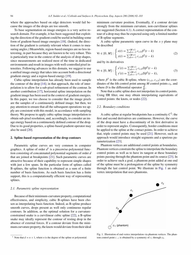
Phantom vertices are additional control points at boundaries.hantom vertices constrain the spline to interpolate the boundaryontrol points as well as to have its tangent at these boundaryoints passing through the phantom point and its source [23]. Inrder to achieve such a goal, a phantom point added at one endf the spline must be a prolongation of the spline by symmetryhrough the last control point. We illustrate in Fig. 1 an end-ertex interpolation that uses phantoms.
ig. 1. Illustration of end-vertex interpolation via phantom vertices. The phan-om control point c−1 is obtained by a symmetry of c1 through c0.
A.F. Stalder et al. / Colloids and Surfaces A: Physicochem. Eng. Aspects 286 (2006) 92–103 95
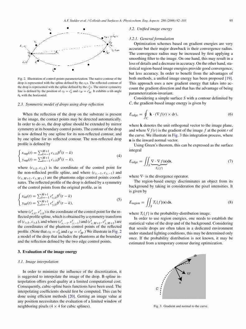
Fig. 2. Illustration of control-points parameterization. The native contour of thedrop is represented with the spline defined by the cks. The reflected contour ofthe drop is represented with the spline defined by the cr
ks. The mirror symmetry
line is defined by the position of c0 = cr0 and cM = cr
M . It exhibits a tilt-angleθh with the horizontal.
2.3. Symmetric model of drops using drop reflection
When the reflection of the drop on the substrate is presentin the image, the contact points may be detected automatically.In order to do so, the drop spline should be extended by mirrorsymmetry at its boundary control points. The contour of the dropis now defined by one spline for its non-reflected contour, andby one spline for its reflected contour. The non-reflected dropprofile is defined by{
xsup(t) =∑M+1k=−1 cx,kβ
3(t − k)
ysup(t) =∑M+1k=−1 cy,kβ
3(t − k),(4)
where (cx,k, cy,k) is the coordinate of the control point forthe non-reflected profile spline, and where (cx,−1, cy,−1) and(cx,M+1, cy,M+1) are the phantoms edge control points coordi-nates. The reflected profile of the drop is defined by a symmetryof the control points from the original profile, as in{
xinf(t) =∑M+1k=−1 cr
x,kβ3(t − k)
yinf(t) =∑M+1k=−1 cr
y,kβ3(t − k),
(5)
where (crx,k, c
ry,k) is the coordinate of the control point for the re-
flected profile spline, which is obtained by a symmetry transformof (cx,k, cy,k), and where (cr
x,−1, cry,−1) and (cr
x,M+1, cry,M+1) are
the coordinates of the phantom control points of the reflected
3.2. Unified image energy
3.2.1. General formulationOptimization schemes based on gradient energies are very
accurate but their major drawback is their convergence radius.The convergence radius may be increased by first applying asmoothing filter to the image. On one hand, this may result in aloss of details and a decrease in accuracy. On the other hand, sta-tistical region-based image energies provide good convergence,but less accuracy. In order to benefit from the advantages ofboth methods, a unified image energy has been proposed [19].This approach uses a new gradient energy that takes into ac-count the gradient direction and that has the advantage of beingparameterization-invariant.
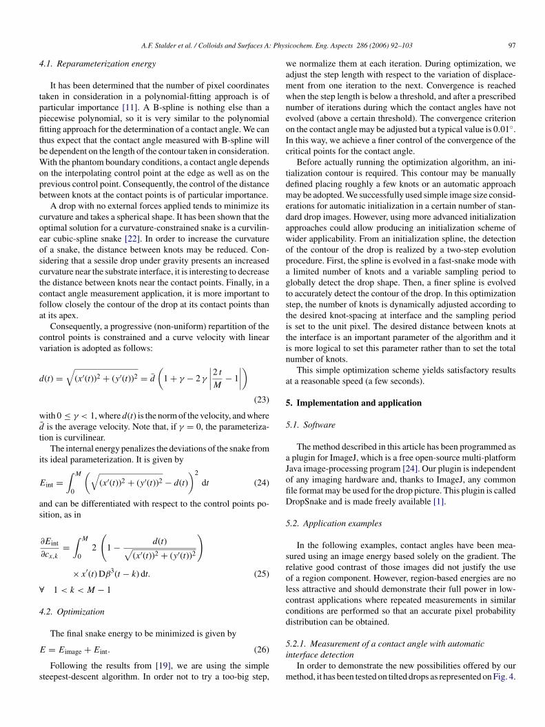
Considering a simple surface S with a contour delimited byC, the gradient-based image energy is given by
Eedge =∮
C
k · (∇f (r) × dr), (6)
where k denotes the unit orthogonal vector to the image plane,and where ∇f (r) is the gradient of the image f at the point r ofthe curve. We illustrate in Fig. 3 this integration process, wheren is the inward normal vector.
Using Green’s theorem, this can be expressed as the surfaceintegral
profile. (Note that c0 = cr0 and cM = cr
M .) We illustrate in Fig. 2a model of the drop that includes the phantoms at the boundaryand the reflection defined by the two edge control points.
3. Evaluation of the image energy
3.1. Image interpolation
In order to minimize the influence of the discretization, itis suggested to interpolate the image of the drop. B-spline in-terpolation offers good quality at a limited computational cost.Consequently, cubic-spline basis functions have been used. Theinterpolating coefficients should first be computed. This can bedone using efficient methods [20]. Getting an image value atany position necessitates the evaluation of a limited window ofneighboring pixels (4 × 4 for cubic splines).
Eedge =∫∫
S
∇ · ∇f (s)︸ ︷︷ ︸Te{f }
ds, (7)
where ∇· is the divergence operator.The region-based energy discriminates an object from its
background by taking in consideration the pixel intensities. Itis given by
Eregion =∫∫
S
Tr{f }(s) ds, (8)
where Tr{f } is the probability-distribution image.In order to use region energies, one needs to establish the
statistical value of the drop and of the background. Consideringthat sessile drops are often taken in a dedicated environmentunder standard lighting conditions, this may be determined onlyonce. If the probability distribution is not known, it may beestimated from a temporary contour during optimization.
Fig. 3. Gradient and normal to the curve.
96 A.F. Stalder et al. / Colloids and Surfaces A: Physicochem. Eng. Aspects 286 (2006) 92–103
Having expressed the gradient energy as a surface integral,the unified image energy may be obtained as
Eimage =∫∫
S
fu(s) ds, (9)
where fu = α Te{f } + (1 − α) Tr{f }. Using Green’s theoremagain, this unified energy may also be rewritten as the contourintegral
Eimage =∮
C
fyu (x, y) dx = −
∮C
fxu (x, y) dy, (10)
where
fyu (x, y) =
∫ x
−∞fu(x, τ) dτ (11)
fxu (x, y) =
∫ y
−∞fu(τ, y) dτ. (12)
3.2.2. Spline parameterization of dropsLet us define Csup and Cinf so that they represent the non-
reflected profile and the reflected profile, respectively, withC = Csup ∪ Cinf. The image energy then becomes
Eimage =∫
Csup
fyu (x, y) dx +
∫Cinf
fyu (x, y) dx (13)
= −∫
fxu (x, y) dy −
∫fx
u (x, y) dy, (14)
o
E
E
3
3
mc
r
3.3.2. Derivation for the axis of symmetryThe positions of c0 and cM are of great importance as they
define the position of the whole reflected profile. Furthermore,the position of these points is greatly influencing the contactangle. Consequently, in order to let them adjust to the imageenergy in the best way, and considering that the symmetry axisis almost horizontal, only their vertical derivative is affected bythe symmetry derivative.
The position (xh, yh) is defined in the middle of the controlpoints c0 and cM . The angle of the axis of symmetry with thehorizontal may then be written as
tan θh = cy,M − cy,0
cx,M − cx,0. (18)
We can derive the image energy with respect to the position ofthese boundary control points as follows:
∂Eimage
∂cy,0= ∂Eimage
∂yh
∂yh
∂cy,0+ ∂Eimage
∂θh
∂θh
∂cy,0(19)
∂Eimage
∂cy,M
= ∂Eimage
∂yh
∂yh
∂cy,M
+ ∂Eimage
∂θh
∂θh
∂cy,M
, (20)
where
∂yh = ∂yh = 1. (21)
U
TA
4
amSutaarsiwBmw[
arw
Csup Cinf
r, using the parametric representation,
image =∫ M
0fysup
u (xsup, ysup)∂xsup
∂tdt
+∫ M
0fyinf
u (xinf, yinf)∂xinf
∂tdt (15)
image =∫ M
0fxsup
u (xsup, ysup)∂ysup
∂tdt
+∫ M
0fxinf
u (xinf, yinf)∂yinf
∂tdt. (16)
.3. Energy derivation
.3.1. Derivation for normal control points
Using (16) and∂f x
u
∂x= fu, the derivative of the image energy
ay be calculated with respect to the horizontal position of aontrol point as
∂Eimage
∂cx,k
= −∮
C
fu∂x
∂cx,k
dy
= −∫ M
0fu
∂xsup
∂crx,k
∂ysup
∂tdt −
∫ M
0fu
∂xinf
∂crx,k
∂yinf
∂tdt.
(17)
Note that the computation of∂Eimage
∂cx,k
and of∂Eimage∂cy,k
can be
ealized efficiently (see Appendix A).
∂cy,0 ∂cy,M 2
sing (18), we finally get
∂θh
∂cy,0= − ∂θh
∂cy,M
= cos2 θh
cx,0 − cx,M
. (22)
he efficient computation of∂Eimage
∂yhand of
∂Eimage∂θh
is reported inppendix B.
. B-Snake
Active contours, or snakes, are widely used in computer-ssisted tools for segmentation. Some of their applications areedical image analysis or feature tracking in video sequences.nakes were originally defined as a spline energy minimizationnder internal and external forces [13]. These forces provide athe same time a way to ensure the smoothness of the curve andway to adapt to specific features. B-spline snakes (B-snakes)
re a particular category of snakes that use a parametric B-splineepresentation of the curve. While having the same basic philo-ophy than snakes, they incorporate the smoothness constraintn an implicit fashion. Thus, they provide a very intuitive model,hich also requires fewer parameters and is consequently faster.-snake formulation is further justified by the fact that the opti-al solution for a curvature-constrained snake is a cubic splinehich may be easily represented using B-spline basis functions
22].In our implementation, external forces are governing the im-
ge energy from Section 3.2. A re-parameterization energy isequired for the snake to keep its smoothness (internal energy),hich we describe now.
A.F. Stalder et al. / Colloids and Surfaces A: Physicochem. Eng. Aspects 286 (2006) 92–103 97
4.1. Reparameterization energy
It has been determined that the number of pixel coordinatestaken in consideration in a polynomial-fitting approach is ofparticular importance [11]. A B-spline is nothing else than apiecewise polynomial, so it is very similar to the polynomialfitting approach for the determination of a contact angle. We canthus expect that the contact angle measured with B-spline willbe dependent on the length of the contour taken in consideration.With the phantom boundary conditions, a contact angle dependson the interpolating control point at the edge as well as on theprevious control point. Consequently, the control of the distancebetween knots at the contact points is of particular importance.
A drop with no external forces applied tends to minimize itscurvature and takes a spherical shape. It has been shown that theoptimal solution for a curvature-constrained snake is a curvilin-ear cubic-spline snake [22]. In order to increase the curvatureof a snake, the distance between knots may be reduced. Con-sidering that a sessile drop under gravity presents an increasedcurvature near the substrate interface, it is interesting to decreasethe distance between knots near the contact points. Finally, in acontact angle measurement application, it is more important tofollow closely the contour of the drop at its contact points thanat its apex.
Consequently, a progressive (non-uniform) repartition of thecontrol points is constrained and a curve velocity with linearv
d
wd
t
i
E
as
∀
4
E
s
we normalize them at each iteration. During optimization, weadjust the step length with respect to the variation of displace-ment from one iteration to the next. Convergence is reachedwhen the step length is below a threshold, and after a prescribednumber of iterations during which the contact angles have notevolved (above a certain threshold). The convergence criterionon the contact angle may be adjusted but a typical value is 0.01◦.In this way, we achieve a finer control of the convergence of thecritical points for the contact angle.
Before actually running the optimization algorithm, an ini-tialization contour is required. This contour may be manuallydefined placing roughly a few knots or an automatic approachmay be adopted. We successfully used simple image size consid-erations for automatic initialization in a certain number of stan-dard drop images. However, using more advanced initializationapproaches could allow producing an initialization scheme ofwider applicability. From an initialization spline, the detectionof the contour of the drop is realized by a two-step evolutionprocedure. First, the spline is evolved in a fast-snake mode witha limited number of knots and a variable sampling period toglobally detect the drop shape. Then, a finer spline is evolvedto accurately detect the contour of the drop. In this optimizationstep, the number of knots is dynamically adjusted according tothe desired knot-spacing at interface and the sampling periodis set to the unit pixel. The desired distance between knots atthe interface is an important parameter of the algorithm and itin
a
5
5
aJofiD
5
srolccd
5i
m
ariation is adopted as follows:
(t) =√
(x′(t))2 + (y′(t))2 = d
(1 + γ − 2 γ
∣∣∣∣2 t
M− 1
∣∣∣∣)
(23)
ith 0 ≤ γ < 1, where d(t) is the norm of the velocity, and where¯ is the average velocity. Note that, if γ = 0, the parameteriza-ion is curvilinear.
The internal energy penalizes the deviations of the snake fromts ideal parameterization. It is given by
int =∫ M
0
(√(x′(t))2 + (y′(t))2 − d(t)
)2
dt (24)
nd can be differentiated with respect to the control points po-ition, as in
∂Eint
∂cx,k
=∫ M
02
(1 − d(t)√
(x′(t))2 + (y′(t))2
)
× x′(t) Dβ3(t − k) dt. (25)
1 < k < M − 1
.2. Optimization
The final snake energy to be minimized is given by
= Eimage + Eint. (26)
Following the results from [19], we are using the simpleteepest-descent algorithm. In order not to try a too-big step,
s more logical to set this parameter rather than to set the totalumber of knots.
This simple optimization scheme yields satisfactory resultst a reasonable speed (a few seconds).
. Implementation and application
.1. Software
The method described in this article has been programmed asplugin for ImageJ, which is a free open-source multi-platform
ava image-processing program [24]. Our plugin is independentf any imaging hardware and, thanks to ImageJ, any commonle format may be used for the drop picture. This plugin is calledropSnake and is made freely available [1].
.2. Application examples
In the following examples, contact angles have been mea-ured using an image energy based solely on the gradient. Theelative good contrast of those images did not justify the usef a region component. However, region-based energies are noess attractive and should demonstrate their full power in low-ontrast applications where repeated measurements in similaronditions are performed so that an accurate pixel probabilityistribution can be obtained.
.2.1. Measurement of a contact angle with automaticnterface detection
In order to demonstrate the new possibilities offered by ourethod, it has been tested on tilted drops as represented on Fig. 4.
98 A.F. Stalder et al. / Colloids and Surfaces A: Physicochem. Eng. Aspects 286 (2006) 92–103
Fig. 4. Drop of ultra-pure water (resistivity 18 Mohms cm, produced by a Mil-lipore MilliQ device, 7–8 �l) on a vertical PMMA substrate (by Goodfellow,research grad). Picture is courtesy of M. Brugnara, Polymers and CompositesLaboratory, University of Trento, Trento, Italy.
In the setup used, the camera is fixed to the sample holder whichcan be rotated. Due to a small misalignment of the camera hori-zontal axis with the substrate, the line passing through the con-tact points reveals a small tilt angle with respect to the horizontalaxis of the image. There is a limited drop reflection on the sub-strate. This image was taken with a digital camera (Nikon995)connected to a 10× lens. The drop had back-light illumination.After selection of the relevant part of the image, the size of theimage was 924 × 650 pixel.
The contour of the drop was determined using the follow-ing parameters: fast snake with 6 knots after manual initializa-tion, Laplacian smoothing-filter radius of 2.0 pixel, gradient-only image energy, knot-spacing constraint at interface 20pixel, knot-spacing ratio 2.0 (γ = 1/3), energy normalizationEint/Eimage = 0.3, convergence criterion 0.01◦. The averagecomputation time was 3 s on a Pentium IV 2 GHz.
The detected drop contour is represented in Fig. 5. The mea-sured contact angles for this example are 98.964◦ and 66.486◦.The detected camera tilt angle was 0.2◦.
Fos
Fig. 6. Advancing angles. The dots represent the positions of the knots. Thetangents at the contact points are represented by the lines. CA stands for contactangle.
5.2.2. Measurement of contact angles for projected dropsAs a second example to illustrate the potential of our method,
we show contact angle measurements on projected, and thereforedeformed, water droplets. The droplet deformation originatesmainly from the inhomogeneous detachment of the droplet fromthe liquid supply needle by an air flow. The air flow is guidedalong the needle using a tube that has a diameter slightly largerthan the needle. The air flow is launched for 50 ms by an elec-tric valve operated by a function generator. The pressure in the
Fta
ig. 5. Detected drop contour and contact angles. The dots represent the positionf the knots. The tangents at the contact points are represented by the lines. CAtands for contact angle.
ig. 7. Receding angles. The dots represent the positions of the knots. Theangents at the contact points are represented by the lines. CA stands for contactngle.
A.F. Stalder et al. / Colloids and Surfaces A: Physicochem. Eng. Aspects 286 (2006) 92–103 99
air tube is adjusted between 80 and 135 mbar, which results ina speed of detached droplet of 0.28 and 0.8 m/s, respectively.The outer needle diameter is 260 µm, and the droplet diameterranges from 1 to 1.4 mm. The flight and the impact of the dropleton the surface was followed by a high-speed camera (PhotronFastcam) at a rate of 10,000 image/s. The droplet shapes arechanging during flight, at impact, and bouncing. The dropletedges are then partially out of focus, making them blurry andnoisy. The snake-based algorithm allows the exact determina-tion of contact angles from blurred images. The development ofdynamic contact angles at surface impact (advancing and reced-ing contact angles, Figs. 6 and 7, respectively) can therefore bestudied in detail.
The contour of the drop was determined using the follow-ing parameters: fast snake with 5 knots after manual initializa-tion, Laplacian smoothing-filter radius of 2.0 pixel, gradient-only image energy, knot-spacing constraint at interface 20pixel, knot-spacing ratio 2.0 (γ = 1/3), energy normalizationEint/Eimage = 0.3, convergence criterion 0.01◦.
5.3. Robustness experiments
In order to evaluate the robustness of our image-energy andcontact angle-measurement approach, various filters have beenapplied to synthetic drop data. The synthetic data set consisted of
Fig. 9. Contact angle error vs. applied noise.
Fig. 10. Image of a synthetic drop with perfect reflection.
Logically, the contact angles near 90◦ should not be muchaffected by the smoothing filter. Angles above 90◦ tend to be in-creased while angles below 90◦ tend to be decreased. It shouldbe noted that the measured contact angles remain within a rea-sonable interval of ±0.36◦ for a Gaussian-filter radius of up to2 pixel.
5.3.2. Robustness to noiseUsing the same synthetic data, we have assessed the effect
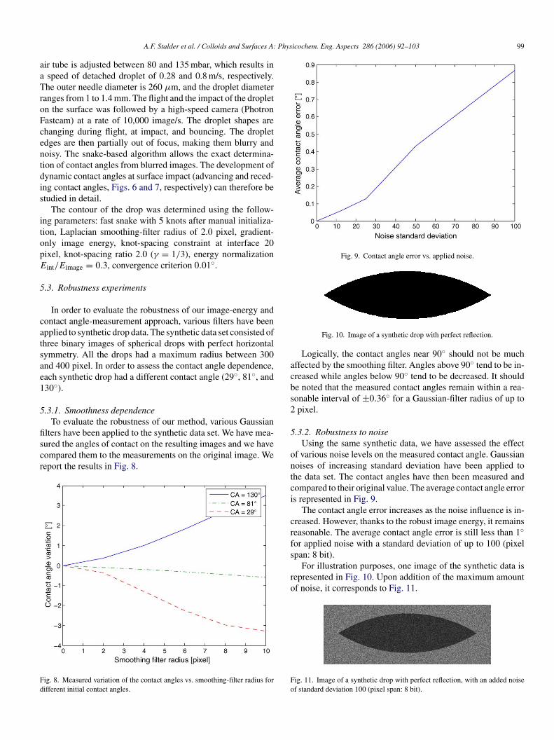
of various noise levels on the measured contact angle. Gaussiannoises of increasing standard deviation have been applied tothe data set. The contact angles have then been measured andcompared to their original value. The average contact angle erroris represented in Fig. 9.
The contact angle error increases as the noise influence is in-creased. However, thanks to the robust image energy, it remainsreasonable. The average contact angle error is still less than 1◦for applied noise with a standard deviation of up to 100 (pixelspan: 8 bit).
For illustration purposes, one image of the synthetic data isrepresented in Fig. 10. Upon addition of the maximum amountof noise, it corresponds to Fig. 11.
Fo
ig. 11. Image of a synthetic drop with perfect reflection, with an added noisef standard deviation 100 (pixel span: 8 bit).
three binary images of spherical drops with perfect horizontalsymmetry. All the drops had a maximum radius between 300and 400 pixel. In order to assess the contact angle dependence,each synthetic drop had a different contact angle (29◦, 81◦, and130◦).
5.3.1. Smoothness dependenceTo evaluate the robustness of our method, various Gaussian
filters have been applied to the synthetic data set. We have mea-sured the angles of contact on the resulting images and we havecompared them to the measurements on the original image. Wereport the results in Fig. 8.
Fig. 8. Measured variation of the contact angles vs. smoothing-filter radius fordifferent initial contact angles.
100 A.F. Stalder et al. / Colloids and Surfaces A: Physicochem. Eng. Aspects 286 (2006) 92–103
Fig. 12. Contact angle variation vs. inter-knot distance. The contact angle vari-ation is given in reference to the contact angle at 20.9 pixel inter-knot distance.
5.4. Inter-knot distance
The contact angle dependence on the distance between knotshas been assessed on the drop from Section 5.2.1. Thanks to thevariety of contact angles that this drop provides, we can evaluatethe influence of the inter-knot distance for angles below andabove 90◦ on the same image. In order to represent clearly theeffect of a lack of control points, the image from Section 5.2.1has been resized to 231 × 162. Indeed, with a smaller resolution,there is less control points for a same inter-knot distance. As thedistance between knots may not always be constant around thedrop profile, the distance between knots at the contact pointsis taken into consideration. The contact angle variation withrespect to the distance between knots at the contact points isrepresented on Fig. 12.
Fig. 12, is giving contact angle evolution with progressinginter-knot distance. The contact angles for a 20.9 pixel knot dis-tance have been taken as reference subsequently. At very smallinter-knot distance, both contact angles could be visually re-jected. Indeed, due to the discrete property of images, consid-ering a too short segment of the contour in the contact angledetermination may result in erroneous results (in spite of thesub-pixel interpolation). In addition, due to the limited contrastat the contact points, the contact angle may become uncertain fortoo small inter-knot distances. This is particularly visible for thesmall contact angle on Fig. 12. At very large inter-knot distance,wkidfomdllv
the curve corresponding to the largest contact angle is decreasingmuch faster.
With reasonable inter-knot distances, a limited dependenceof contact angles on inter-knot distance is observed. As a con-sequence, it is important to keep this parameter fixed for allmeasurements within a study. The inter-knot distance should beset above a minimum value allowing a reasonable pixel aver-aging. However, it should allow a sufficient number of knots inorder to correctly follow the drop contour. The latter point rep-resents normally no problem and is easy to ensure (10 knots arenormally enough). We typically use an inter-knot distance of 20pixel in our studies.
5.5. Software evaluation
Comparison between contact angle measurements methodsis a challenging task. Indeed, different methods make differ-ent assumptions (e.g., axisymmetricity), necessitates differentinputs (e.g., automatic or manual positioning of the substratelevel) and can give extra informations (e.g., capillary constantwith ADSA). In addition, results can be highly dependent ona particular software application and a same drop model canbe used with several edge detection methods sometimes. How-ever, in order to give an evaluation of the implementation ofthe method, comparisons have been performed with other meth-ods for which the software implementation was available to us.TssaiIdaTfR
oaRruo
aibmtssmamri
e also observe an increased contact angle variability when thenots can no more represent correctly the drop contour. For annter-knot spacing of about 60 pixel, there was only 5 knots toefine the drop contour at this resolution. The maximum limitor the inter-knot distance is related to the minimum numberf knots required to accurately represent a drop contour. Thisinimum number of knots is independent of the resolution but
epends on the total curvature of the drop. Thus, the maximumimit on the inter-knot distance may be more easily reached atimited resolution or large contact angles. We see indeed that atery high inter-knot distances both contact angles decrease, but
hus, this subsection cannot claim to compare methods but onlyoftware applications based on different methods. In this sub-ection, we refer to axisymmetric for our implementation ofn axis-symmetric method based on Laplace equation. Our ax-symmetric implementation was done as a plugin for ImageJ.t is largely based on [10,9] but uses a segmentation methodepending on thresholded gradient. This latter point results inslight overestimation of the contour and of the contact angle.he measurements based on the polynomial method were per-
ormed with a commercial software (Windrop++ V4.10, GBX,omans-sur-Isere, France).
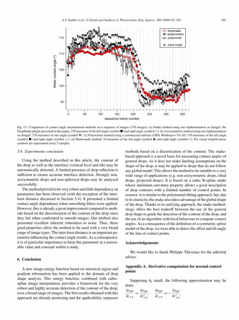
Dynamic contact angles were measured on the same sequencef a drop of water on an isotropic silicium substrate. Images werecquired on a commercial contact angle meter (Digidrop, GBX,omans-sur-Isere, France). For Dropsnake and the axisymmet-
ic method, the initialization on each frame but the first wassing the solution of the preceding frame. Results are presentedn Fig. 13.
Considering the offset of our axisymmetric implementation,bsolute contact angle considerations may difficultly be takennto account. However, the stability of the measurements maye evaluated. The DropSnake curve is relatively smooth and itseasurements are much more stable than measurements from
he other methods. In the area of receding angle (frame 270–320)tandard deviations were measured to be 0.2◦, 0.6◦ and 1.3◦, re-pectively for DropSnake, the axisymmetric and the polynomialethod. It should be noted as well that according to DropSnake
nd the polynomial method, the drop is not perfectly axisym-etric although it was supposed to be. This latter aspect appears
edundantly in our studies as isotropicity is hard to achieve dur-ng surface preparation and contact angle measurement.
A.F. Stalder et al. / Colloids and Surfaces A: Physicochem. Eng. Aspects 286 (2006) 92–103 101
Using the method described in this article, the contour ofthe drop as well as the interface (vertical level and tilt) may beautomatically detected. A limited presence of drop reflection issufficient to ensure accurate interface detection. Strongly non-axisymmetric drops and non-spherical drops may be analyzedsuccessfully.
The method proved to be very robust and little dependency onparameters has been observed (with the exception of the inter-knot distance discussed in Section 5.4). It presented a limitedcontact angle dependence when smoothing filters were applied.However, this is already a great improvement compared to meth-ods based on the discretization of the contour of the drop sincethey fail when confronted to smooth images. Our method alsopresented excellent inherent robustness to noise. Thus, thesegood properties allow the method to be used with a very broadrange of image types. The inter-knot distance is an important pa-rameter influencing the contact angle results. As a consequence,it is of particular importance to keep this parameter at a reason-able value and constant within a study.
6. Conclusion
A new image energy function based on statistical region andgssroa
methods based on a discretization of the contour. The snake-based approach is a novel basis for measuring contact angles ofgeneral drops. As it does not make limiting assumptions on theshape of the drop, it may be applied to drops that do not followany global model. This allows the method to be suitable to a verywide range of applications (e.g. non-axisymmetric drops, tilteddrops, projected drops). It is based on a cubic B-spline snakewhose minimum-curvature property allows a good descriptionof drop contours with a limited number of control points. Inessence, it is similar to the polynomial-fitting approach, but, dueto its elasticity, the snake also takes advantage of the global shapeof the drop. Thanks to its unifying approach, the snake method-ology offers the best tradeoff between the use of the generaldrop shape to guide the detection of the contour of the drop, andthe use of an algorithm with local behaviour to compute contactangles. As a consequence of the definition of a symmetric splinemodel of the drop, we were able to detect the offset and tilt angleof the line of contact points.
Acknowledgements
We would like to thank Philippe Thevenaz for the editorialadvice.
Appendix A. Derivative computation for normal controlpoints
d
radient information has been applied to the domain of drophape analysis. This energy function, combined with cubic-pline image interpolation, provides a framework for the veryobust and highly accurate detection of the contour of the drop,ver a broad range of images. The first results obtained with thispproach are already promising and the applicability surpasses
Supposing θh small, the following approximation may beone:∂xinf
∂cx,k
= ∂xinf
∂crx,k
,∂yinf
∂cy,k
= − ∂yinf
∂cry,k
.
102 A.F. Stalder et al. / Colloids and Surfaces A: Physicochem. Eng. Aspects 286 (2006) 92–103
The energy derivative (17) may be rewritten as:
∂Eimage
∂cx,k
= −M+1∑l=−1
[cy,l
∫ M
0fu
∂xsup
∂cx,k
Dβ3(t − l)dt
− cry,l
∫ M
0fu
∂xinf
∂crx,k
Dβ3(t − l)dt
](A.1)
Note that:∂xsup
∂cx,k
= ∂ysup
∂cy,k
= β3(t − k) ∀ 2 ≤ k ≤ M − 2 (A.2)
and due to the phantom edge definition:
∂xsup
∂cx,1= ∂ysup
∂cy,1= β3(t − 1) − β3(t + 1)
∂xsup
∂cx,0= ∂ysup
∂cy,0= β3(t) + 2β3(t + 1)
∂xsup
∂cx,M−1= ∂ysup
∂cy,M−1= β3(t − (M − 1))
− β3(t − (M + 1))∂xsup
∂cx,M
= ∂ysup
∂cy,M
= β3(t − M) + 2β3(t − (M + 1))
(A.3)
The spline representing the reflected contour has identicalderivatives for its respective control points.
ddc
sicim
As
The image derivative energy with respect to the angle θh maybe written as an average of its computations using f
yu and fx
u :
∂Eimage
∂θh= 1
2
∫ M
0
(∂f
yu
∂y
∂yinf
∂θh+ ∂f
yu
∂x
∂xinf
∂θh
)∂xinf
∂tdt
+ 1
2
∫ M
0
(∂f x
u
∂x
∂xinf
∂θh+ ∂f x
u
∂y
∂yinf
∂θh
)∂yinf
∂tdt (B.2)
Which can be rearranged as:
∂Eimage
∂θh= 1
2
∫ M
0
[(∂f
yu
∂y
∂xinf
∂t+ ∂f x
u
∂y
∂yinf
∂t
)∂yinf
∂θh
+(
∂fyu
∂x
∂xinf
∂t+ ∂f x
u
∂x
∂yinf
∂t
)∂xinf
∂θh
]dt (B.3)
The terms ∂fyu
∂xand ∂f x
u
∂ymay be computed, however that would
require twice the computation over the whole image. In practice,if we are close enough to the drop, the path should remain parallelto the contour and its energy image. That means that the productof the differentiation of the energy image in a direction and thedisplacement in the same direction should remain small. Hence,
we neglect the products ∂f xu
∂y∂yinf∂t
and ∂fyu
∂x∂xinf∂t
.The computed derivative is then:
Note that the cubic spline basis function β3 as well as itserivative Dβ3 have a finite support and the integral in (A.1)oes not need to be computed over its whole range. However,are should be taken with the boundaries.
Note also that the integral (A.1) may be calculated as a finiteum. Although the phantom border conditions are complicat-ng the notation, the spline basis function product may be pre-alculated. These computation considerations were thoroughlynvestigated in [19], and the phantoms border conditions are only
aking things (and notation) a little bit more complicated.Similarly, using (15), the y-axis derivative may be obtained:
∂Eimage
∂cy,k
=M+1∑l=−1
[cx,l
∫ M
0fu
∂ysup
∂cx,k
Dβ3(t − l)dt
− crx,l
∫ M
0fu
∂yinf
∂crx,k
Dβ3(t − l)dt
](A.4)
ppendix B. Derivative computation for the axis ofymmetry
Here again, it is supposed that θh is small:∂yinf∂yh
[2] S. Herminghaus, Wetting: introductory note, J. Phys.: Condens. Matter. 17(2005) S261–S264.
[3] T. Young, An essay on the cohesion of fluids, Philos. Trans. R. Soc. Lond.95 (1905) 65–87.
[4] W. Barthlott, C. Neinhuis, The purity of sacred lotus or escape from con-tamination in biological surfaces, Planta 202 (1997) 1–8.
[5] Y.T. Cheng, D.E. Rodak, Is the lotus leaf superhydrophobic?, Appl. Phys.Lett. 86 (2005) 144101.
[6] T. Michel, U. Mock, I. Roisman, J. Ruhe, C. Tropea, The hydrodynamicsof drop impact onto chemically structured surfaces, J. Phys.: Condens.Matter. 17 (2005) S607–S622.
[7] U. Mock, T. Michel, C. Tropea, I. Roisman, J. Ruhe, Drop impact onchemically structured arrays, J. Phys.: Condens. Matter. 17 (2005) S595–S605.
[8] P.G. de Gennes, Wetting: statics and dynamics, Rev. Mod. Phys. 57 (1985)827–863.
[9] Y. Rotenberg, L. Boruvka, A.W. Neumann, Determination of surface ten-sion and contact angle from the shapes of axisymmetric fluid interfaces, J.Colloid Interface Sci. 93 (1983) 169–183.
[10] M. Hoorfar, A.W. Neumann, Axisymmetric drop shape analysis (adsa) forthe determination of surface tension and contact angle, J. Adhesion 80(2004) 727–747.
[11] A. Bateni, S.S. Susnar, A. Amirfazli, A.W. Neumann, A high-accuracypolynomial fitting approach to determine contact angles, Colloids Surf. A219 (2003) 215–231.
[12] O.I. del Rio, D.Y. Kwok, R. Wu, J.M. Alvarez, A.W. Neumann, Contactangle measurement by axisymmetric drop shape analysis and a automatedpolynomial fit program, Colloids Surf. A 143 (1998) 197–210.
A.F. Stalder et al. / Colloids and Surfaces A: Physicochem. Eng. Aspects 286 (2006) 92–103 103
[13] M. Kass, A. Witkin, D. Terzopoulos, Snakes: Active contour models, Int.J. Comput. Vis. (1988) 321–331.
[14] P. Cheng, D. Li, L. Boruvka, Y. Rotenberg, A.W. Neumann, Automation ofaxisymmetric drop shape analysis for measurement of interfacial tensionsand contact angles, Colloids Surf. A 43 (1990) 151–167.
[15] C. Atae-Allah, M. Cabrerizo-Vilchez, J.F. Gomez-Lopera, J.A. Holgado-Terriza, R. Roman-Roldan, P.L. Luque-Escamilla, Measurement of surfacetension and contact angle using entropic edge detection, Meas. Sci. Tech-nol. 12 (2001) 288–298.
[16] M.G. Cabezas, A. Bateni, J.M. Montanero, A.W. Neumann, A new drop-shape methodology for surface tension measurement, Appl. Surf. Sci. 238(2004) 480–484.
[17] M.G. Cabezas, A. Bateni, J.M. Montanero, A.W. Neumann, A new methodof image processing in the analysis of axisymmetric drop shapes, ColloidsSurf. A 255 (2005) 193–200.
[18] H.W. Park, T. Schoepflin, Y. Kim, Active contour model with gradientdirectional information: directional snake, IEEE Trans. Circuits Syst. Vid.11 (2001) 252–256.
[19] M. Jacob, T. Blu, M. Unser, Efficient energies and algorithms for parametricsnakes, IEEE Trans. Image Process. 13 (2004) 1231–1244.
[20] M. Unser, Splines: a perfect fit for signal and image processing, IEEESignal Process. Mag. 16 (1999) 22–38.
[21] A. Blake, M. Isard, Active contours, Springer Verlag, London, 1998.[22] P. Brigger, J. Hoeg, M. Unser, B-Spline snakes: A flexible tool for para-
[23] R. Bartels, J. Beatty, B. Barsky, An introduction to splines for use in com-puter graphics and geometric modeling, Morgan Kaufmann Publishers,Los Altos California, 1987.