TDA Progress Report 42-127 November 15, 1996

A Soft-Input Soft-Output Maximum A Posteriori(MAP) Module to Decode Parallel and

Serial Concatenated CodesS. Benedetto,a D. Divsalar,b G. Montorsi,a and F. Pollarab

Concatenated coding schemes with interleavers consist of a combination of twosimple constituent encoders and an interleaver. The parallel concatenation knownas “turbo code” has been shown to yield remarkable coding gains close to theoreticallimits, yet admitting a relatively simple iterative decoding technique. The recentlyproposed serial concatenation of interleaved codes may offer performance superiorto that of turbo codes. In both coding schemes, the core of the iterative decodingstructure is a soft-input soft-output (SISO) module. In this article, we describethe SISO module in a form that continuously updates the maximum a posteriori(MAP) probabilities of input and output code symbols and show how to embedit into iterative decoders for parallel and serially concatenated codes. Results arefocused on codes yielding very high coding gain for space applications.

I. Introduction

Concatenated coding schemes have been studied by Forney [1] as a class of codes whose probabilityof error decreased exponentially at rates less than capacity, while decoding complexity increased onlyalgebraically. Initially motivated only by theoretical research interests, concatenated codes have sincethen evolved as a standard for those applications where very high coding gains are needed, such as(deep-)space applications.

The recent proposal of “turbo codes” [2], with their astonishing performance close to the theoreticalShannon capacity limits, has once again shown the great potential of coding schemes formed by twoor more codes working in a concurrent way. Turbo codes are parallel concatenated convolutional codes(PCCCs) in which the information bits are first encoded by a recursive systematic convolutional codeand then, after passing through an interleaver, are encoded by a second systematic convolutional encoder.The code sequences are formed by the information bits, followed by the parity check bits generated byboth encoders. Using the same ingredients, namely convolutional encoders and interleavers, seriallyconcatenated convolutional codes (SCCCs) have been shown to yield performance comparable, and insome cases superior, to turbo codes [5].

a Politecnico di Torino, Torino, Italy.

b Communications Systems and Research Section.

1

Both concatenated coding schemes admit a suboptimum decoding process based on the iterations of themaximum a posteriori (MAP) algorithm [12] applied to each constituent code. The purpose of this articleis to describe a soft-input soft-output module (denoted by SISO) that implements the MAP algorithm inits basic form, the extension of it to additive MAP (log-MAP), which is indeed a dual-generalized Viterbialgorithm with correction,1 and finally extension to the continuous decoding of PCCC and SCCC. Asexamples of applications, we will show the results obtained by decoding two low-rate codes, with veryhigh coding gain, aimed at deep-space applications.

II. Iterative Decoding of Parallel and Serial Concatenated Codes

In this section, we show the block diagram of parallel and serially concatenated codes, together withtheir iterative decoders. It is not within the scope of this article to describe and analyze the decodingalgorithms. For them, the reader is directed to [2,4,6,7] (for PCCC) and [3,5,8] (for SCCC). Rather,we aim at showing that both iterative decoding algorithms need a particular module, named soft-input,soft-output (SISO), which implements operations strictly related to the MAP algorithm, and which willbe analyzed in detail in the next section.

A. Parallel Concatenated Codes

The block diagram of a PCCC is shown in Fig. 1 (the same construction also applies to block codes).In the figure, a rate 1/3 PCCC is obtained using two rate 1/2 constituent codes (CCs) and an interleaver.For each input information bit, the codeword sent to the channel is formed by the input bit, followed bythe parity check bits generated by the two encoders. In Fig. 1, the block diagram of the iterative decoderis also shown. It is based on two modules denoted by “SISO,” one for each encoder, an interleaver, and adeinterleaver performing the inverse permutation with respect to the interleaver. The input and outputreliabilities for each SISO module in Fig. 1 are described in Section V.

The SISO module is a four-port device, with two inputs and two outputs. A detailed description of itsoperations is deferred to the next section. Here, it suffices to say that it accepts as inputs the probabilitydistributions of the information and code symbols labeling the edges of the code trellis, and forms asoutputs an update of these distributions based upon the code constraints. It can be seen from Fig. 1 thatthe updated probabilities of the code symbols are never used by the decoding algorithm.

B. Serially Concatenated Codes

The block diagram of a SCCC is shown in Fig. 2 (the same construction also applies to block codes).In the figure, a rate 1/3 SCCC is obtained using as an outer encoder a rate 1/2 encoder, and as aninner encoder a rate 2/3 encoder. An interleaver permutes the output codewords of the outer code beforepassing them to the inner code. In Fig. 2, the block diagram of the iterative decoder is also shown. It isbased on two modules denoted by “SISO,” one for each encoder, an interleaver, and a deinterleaver.

The SISO module is the same as described before. In this case, though, both updated probabilities ofthe input and code symbols are used in the decoding procedure. The input and output reliabilities foreach SISO module in Fig. 2 are described in Section V.

C. Soft-Output algorithms

The SISO module is based on MAP algorithms. MAP algorithms have been known since theearly seventies [10–14]. The algorithms in [11–14] perform both forward and backward recursionsand, thus, require that the whole sequence be received before starting the decoding operations. As a

1 A. J. Viterbi, “An Intuitive Justification and a Simplified Implementation of the MAP Decoder for Convolutional Codes,”submitted to the JSAC issue on “Concatenated Coding Techniques and Iterative Decoding: Sailing Toward ChannelCapacity.”

2

¥

ENCODER1

RATE = 1/2TO CHANNEL

NOT TRANSMITEDENCODER

2RATE = 1/2

TO CHANNEL

(c;O)

TO CHANNEL

NOT USED (c;I)

(u;O) (u;I)

FROMDEMOD

DECISION

SISO2

SISO1

(c;O)

(u;O)

NOT USED

(c;I)

(u;I)

FROMDEMOD

(a)

(b)

–1

Fig. 1. Block diagram of a parallel concatenated convolutional code (PCCC): (a) a PCCC,rate = 1/3 and (b) iterative decoding of a PCCC.

–1

OUTERENCODERRATE = 1/2

(c;O)

TO CHANNEL

(c;I)

(u;O) (u;I)SISO

OUTER

SISOINNER

(c;O)

(u;O)

NOT USED

(c;I)

(u;I)

FROMDEMOD

(a)

(b)

INNERENCODERRATE = 2/3

DECISION

0

Fig. 2. Serially concatenated convolutional code (SCCC): (a) an SCCC, rate = 1/3 and(b) iterative decoding of an SCCC.

3

consequence, they can only be used in block-mode decoding. The memory requirement and computationalcomplexity grow linearly with the sequence length.

The algorithm in [10] requires only a forward recursion, so that it can be used in continuous-modedecoding. However, its memory and computational complexity grow exponentially with the decoding de-lay. Recently, a MAP symbol-by-symbol decoding algorithm conjugating the positive aspects of previousalgorithms, i.e., a fixed delay and linear memory and complexity growth with decoding delay, has beenproposed in [15].

All previously described algorithms are truly MAP algorithms. To reduce the computational com-plexity, various forms of suboptimum soft-output algorithms have been proposed. Two approaches havebeen taken. The first approach tries to modify the Viterbi algorithm. Forney considered “augmentedoutputs” from the Viterbi algorithm [16]. These augmented outputs include the depth at which all pathsare merged, the difference in length between the best and the next-best paths at the point of merging,and a given number of the most likely path sequences. The same concept of augmented output waslater generalized for various applications [17–21]. A different approach to the modification of the Viterbialgorithm was followed in [22]. It consists of generating a reliability value for each bit of the hard-outputsignal and is called the soft-output Viterbi algorithm (SOVA). In the binary case, the degradation ofSOVA with respect to MAP is small [23]; however, SOVA is not as effective in the nonbinary case. Acomparison of several suboptimum soft-output algorithms can be found in [24]. The second approachconsists of revisiting the original symbol MAP decoding algorithms [10,12] with the aim of simplifyingthem to a form suitable for implementation [15,25–30].

III. The SISO Module

A. The Encoder

The decoding algorithm underlying the behavior of SISO works for codes admitting a trellis represen-tation. It can be a time-invariant or time-varying trellis, and, thus, the algorithm can be used for bothblock and convolutional codes. In the following, for simplicity of the exposition, we will refer to the caseof time-invariant convolutional codes.

In Fig. 3, we show a trellis encoder, characterized by the following quantities:2

(1) U = (Uk)k∈K is the sequences of input symbols, defined over a time index set K (finiteor infinite) and drawn from the alphabet

U = {u1, . . . , uNI}

To the sequence of input symbols, we associate the sequence of a priori probabilitydistributions:

P(u; I) = (Pk(uk; I))k∈K

2 In the following, capital letters U,C, S,E will denote random variables and lower-case letters u, c, s, e their realizations.The roman letter P[A] will denote the probability of the event A, whereas the letter P (a) (italic) will denote a functionof a. The subscript k will denote a discrete time, defined on the time index set K. Other subscripts, like i, will refer toelements of a finite set. Also, “()” will denote a time sequence, whereas “{}” will denote a finite set of elements.

4

where

Pk(uk; I) 4= P[Uk = uk]

(2) C = (Ck)k∈K is the sequences of output, or code, symbols, defined over the same timeindex set K, and drawn from the alphabet

C = {c1, . . . , cNO}

To the sequence of output symbols, we associate the sequence of a priori probabilitydistributions:

P(c; I) = (Pk(ck; I))k∈K

For simplicity of notation, we drop the dependency of uk and ck on k. Thus, Pk(uk; I)and Pk(ck; I) will be denoted simply by Pk(u; I) and Pk(c; I), respectively.

Fig. 3. The trellis encoder.

TRELLISENCODER

INPUT

U

OUTPUT

C

B. The Trellis Section

The dynamics of a time-invariant convolutional code are completely specified by a single trellis section,which describes the transitions (edges) between the states of the trellis at time instants k and k + 1. Atrellis section is characterized by the following:

(1) A set of N states S = {s1, . . . , sN}. The state of the trellis at time k is Sk = s, withs ∈ S.

(2) A set of N ×NI edges obtained by the Cartesian product

E = S × U = {e1, . . . , eN×NI}

which represents all possible transitions between the trellis states.

The following functions are associated with each edge e ∈ E (see Fig. 4):

(1) The starting state sS(e) (the projection of e onto S).

(2) The ending state sE(e).

(3) The input symbol u(e) (the projection of e onto U).

(4) The output symbol c(e).

5

sS(e)

e

u (e), c (e)

s E(e)

Fig. 4. An edge of the trellis section.

The relationship between these functions depends on the particular encoder. As an example, in thecase of systematic encoders, (sE(e), c(e)) also identifies the edge since u(e) is uniquely determined by c(e).In the following, we only assume that the pair (sS(e), u(e)) uniquely identifies the ending state sE(e);this assumption is always verified, as it is equivalent to say that, given the initial trellis state, there is aone-to-one correspondence between input sequences and state sequences, a property required for the codeto be uniquely decodable.

C. The SISO Algorithm

The SISO module is a four-port device that accepts at the input the sequences of probability distri-butions

P(c; I) P(u; I)

and outputs the sequences of probability distributions

P(c;O) P(u;O)

based on its inputs and on its knowledge of the trellis section (or code in general).

We assume first that the time index set K is finite, i.e., K = {1, . . . , n}. The algorithm by which theSISO operates in evaluating the output distributions will be explained in two steps. In the first step, weconsider the following algorithm:

(1) At time k, the output probability distributions are computed as

Pk(c;O) = Hc

∑e:c(e)=c

Ak−1[sS(e)]Pk[u(e); I]Pk[c(e); I]Bk[sE(e)] (1)

Pk(u;O) = Hu

∑e:u(e)=u

Ak−1[sS(e)]Pk[u(e); I]Pk[c(e); I]Bk[sE(e)] (2)

6

(2) The quantities Ak(·) and Bk(·) are obtained through the forward and backward recur-sions, respectively, as

Ak(s) =∑

e:sE(e)=s

Ak−1[sS(e)]Pk[u(e); I]Pk[c(e); I] , k = 1, . . . , n (3)

Bk(s) =∑

e:sS(e)=s

Bk+1[sE(e)]Pk+1[u(e); I]Pk+1[c(e); I] , k = n− 1, . . . , 0 (4)

with initial values

A0(s) ={ 1 s = S0

0 otherwise(5)

Bn(s) ={ 1 s = Sn

0 otherwise(6)

The quantities Hc, Hu are normalization constants defined as follows:

Hc →∑c

Pk(c;O) = 1

Hu →∑u

Pk(u;O) = 1

In the second step, from Eqs. (1) and (2), it is apparent that the quantities Pk[c(e); I] in the firstequation and Pk[u(e); I] in the second do not depend on e, by definition of the summation indices, andthus can be extracted from the summations. Thus, defining the new quantities

Pk(c;O) 4= HcPk(c;O)Pk(c; I)

Pk(u;O) 4= HuPk(u;O)Pk(u; I)

where Hc and Hu are normalization constants such that

Hc →∑c

Pk(c;O) = 1

Hu →∑u

Pk(u;O) = 1

it can be easily verified that they can be obtained through the expressions

7

Pk(c;O) = HcHc

∑e:c(e)=c

Ak−1[sS(e)]Pk[u(e); I]Bk[sE(e)] (7)

Pk(u;O) = HuHu

∑e:u(e)=u

Ak−1[sS(e)]Pk[c(e); I]Bk[sE(e)] (8)

where the A’s and B’s satisfy the same recursions previously introduced in Eq. (3).

The new probability distributions Pk(u;O) and Pk(c;O) represent a smoothed version of the inputdistributions Pk(c; I) and Pk(u; I), based on the code constraints and obtained using the probabilitydistributions of all symbols of the sequence but the kth ones, Pk(c; I) and Pk(u; I). In the literature ofturbo decoding, Pk(u;O) and Pk(c;O) would be called extrinsic information. They represent the addedvalue of the SISO module to the a priori distributions Pk(u; I) and Pk(c; I). Basing the SISO algorithmon Pk(·;O) instead of on Pk(·;O) simplifies the block diagrams, and related software and hardware, of theiterative schemes for decoding concatenated codes. For this reason, we will consider as an SISO algorithmthe one expressed by Eq. (7). The SISO module is then represented as in Fig. 5.

Previously proposed algorithms were not in a form suitable for working with a general trellis code.Most of them assumed binary input symbols, some also assumed systematic codes, and none (not even theoriginal Bahl–Cocke–Jelinek–Raviv (BCJR) algorithm) could cope with a trellis having parallel edges. Ascan be noticed from all summations involved in the equations that define the SISO algorithm, we work ontrellis edges rather than on pairs of states, and this makes the algorithm completely general and capableof coping with parallel edges and also with encoders with rates greater than one, like those encounteredin some concatenated schemes.

Fig. 5. The soft-input soft-output (SISO model).

SISO

P (c;O )

P (u;O )

P (c;I )

P (u;I )

D. Computation of Input and Output Bit Extrinsic Information

In this subsection, bit extrinsic information is derived from the symbol extrinsic information usingEqs. (7) and (8). Consider a rate ko/no trellis encoder such that each input symbol U consists of ko bitsand each output symbol C consists of no bits. Assume

Pk(c; I) =no∏j=1

Pk,j(cj ; I) (9)

Pk(u; I) =ko∏j=1

Pk,j(uj ; I) (10)

where cj ∈ {0, 1} denotes the value of the jth bit Cjk of the output symbol Ck = c; j = 1, . . . , no,and uj ∈ {0, 1} denotes the value of the jth bit U jk of the input symbol Uk = u; j = 1, . . . , ko. Thisassumption is valid in an iterative decoding when bit interleavers rather than symbol interleavers are used.One should be cautious when using Pk(c; I) as a product for those encoders in a concatenated system

8

where the output C in Fig. 3 is connected to a channel. For such cases, if, for an example, a nonbinaryinput additive white Gaussian noise (AWGN) channel is used, this assumption usually is not needed (thiswill be discussed shortly), and Pk(c; I) = Pk(c|y) = Pk(y|x(c))P (c)/P (y), where y is the complex receivedsample(s) and x(c) is the transmitted nonbinary symbol(s). Then, for binary input memoryless channels,Pk(y|x(c)) can be written as a product. After obtaining symbol probability distributions Pk(c;O) andPk(c;O) from Eqs. (7) and (8) by using Eqs. (2) and (4), it is easy then to show that the input andoutput bit extrinsic information can be obtained as

Pk,j(cj ;O) = Hcj

∑c:Cj

k=cj

Pk(c;O)no∏i=1i6=j

Pk,j(ci; I) (11)

Pk,j(uj ;O) = Huj

∑u:Uj

k=uj

Pk(u;O)ko∏i=1i6=j

Pk,j(ui; I) (12)

where Hcj and Huj are normalization constants such that

Hcj →∑

cj∈{0,1}Pk,j(cj ;O) = 1

Huj →∑

uj∈{0,1}Pk,j(uj ;O) = 1

Equation (11) is not used for those encoders in a concatenated coded system connected to a channel. Tokeep the expressions general, as is seen from Eqs. (3), (4), and (12), Pk[c(e); I] is not represented as aproduct.

Direct computation of the probability distribution of bits without first obtaining the probability distri-bution of symbols is presented in [9]. In the following sections, for simplicity of notation, the probabilitydistribution of symbols rather than of bits is considered. The extension of the results to probabilitydistributions of bits based on the above derivations is straightforward.

IV. The Sliding-Window Soft-Input Soft-Output Module (SW-SISO)

As previous description should have made clear, the SISO algorithm requires that the whole sequencehas been received before starting the smoothing process. The reason is due to the backward recursion thatstarts from the (supposed-known) final trellis state. As a consequence, its practical application is limitedto the case when the duration of the transmission is short (n small) or, for n long, when the receivedsequence can be segmented into independent consecutive blocks, like for block codes or convolutionalcodes with trellis termination. It cannot be used for continuous decoding of convolutional codes. Thisconstraint leads to a frame rigidity imposed on the system and also reduces the overall code rate.

A more flexible decoding strategy is offered by modifying the algorithm in such a way that the SISOmodule operates on a fixed memory span and outputs the smoothed probability distributions after a givendelay, D. We call this new algorithm the sliding-window soft-input soft-output (SW-SISO) algorithm (andmodule). We propose two versions of the SW-SISO that differ in the way they overcome the problemof initializing the backward recursion without waiting for the entire sequence. From now on, we assumethat the time index set K is semi-infinite, i.e., K = {1, . . . ,∞}, and that the initial state s0 is known.

9

A. The First Version of the Sliding-Window SISO Algorithm (SW-SISO1)

The SW-SISO1 algorithm consists of the following steps:

(1) Initialize A0 according to Eq. (5).

(2) Forward recursion at time k: Compute the Ak through the forward recursion of Eq. (3).

(3) Initialization of the backward recursion (time k > D):

B(0)k (s) = Ak(s) ∀s (13)

(4) Backward recursion: It is performed according to Eq. (4) from iterations i = 1 to i = Das

B(i)k−i(s) =

∑e:sS(e)=s

B(i−1)k−i+1[sE(e)]Pk[u(e); I]Pk[c(e); I] (14)

and

Bk−D(s) = B(D)k−D(s) ∀s (15)

(5) The probability distributions at time k −D are computed as

Pk−D(c;O) = HcHc

∑e:c(e)=c

Ak−D−1[sS(e)]Pk−D[u(e); I]Bk−D[sE(e)] (16)

Pk−D(u;O) = HcHc

∑e:u(e)=u

Ak−D−1[sS(e)]Pk−D[c(e); I]Bk−D[sE(e)] (17)

B. The Second Simplified Version of the Sliding-Window SISO Algorithm (SW-SISO2)

A further simplification of the sliding-window SISO algorithm, which is similar to SW-SISO1 exceptfor the backward initial condition, that significantly reduces the memory requirements consists of thefollowing steps:

(1) Initialize A0 according to Eq. (5).

(2) Forward recursion at time k, k > D: Compute the Ak−D through the forward recursion

Ak−D(s) =∑

e:sE(e)=s

Ak−D−1[sS(e)]Pk−D[u(e); I]Pk−D[c(e); I] , k > D (18)

(3) Initialization of the backward recursion (time k > D):

B(0)k (s) =

1N∀s (19)

10

(4) Backward recursion (time k > D): It is performed according to Eq. (14) as before.

(5) The probability distributions at time k−D are computed according to Eqs. (16) and (17)as before.

C. Memory and Computational Complexity

1. Algorithm SW-SISO1. For a convolutional code with parameters (k0, n0) and number of statesN , so that NI = 2k0 and NO = 2n0 , the algorithm SW-SISO1 requires storage of N ×D values of A’s andD(NI + NO) values of the input unconstrained probabilities Pk(u; I) and Pk(c; I). Moreover, to updatethe A’s and B’s for each time instant, it needs to perform 2×N ×NI multiplications and N additions ofNI numbers. To output the set of probability distributions at each time instant, we need a D-times longbackward recursion. Thus, overall the computational complexity requires the following:

(1) 2(D + 1)×N ×NI multiplications.

(2) (D + 1)×N × (NI − 1) additions.

2. Algorithm SW-SISO2. This simplified version of the sliding-window SISO algorithm doesnot require the storage of the N × D values of A’s, as they are updated with a delay of D steps. Asa consequence, only N values of A’s and D(NI + NO) values of the input unconstrained probabilitiesPk(u; I) and Pk(c; I) need to be stored. The computational complexity is the same as that for the previousversion of the algorithm. However, since the initialization of the B recursion is less accurate, a largervalue of D may be necessary.

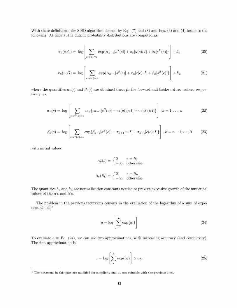
V. The Additive SISO Algorithm (A-SISO)

The sliding-window SISO algorithms solve the problems of continuously updating the probabilitydistributions, without requiring trellis terminations. Their computational complexity, however, is stillhigh when compared to other suboptimal algorithms like SOVA. This is due mainly to the fact thatthey are multiplicative algorithms. In this section, we overcome this drawback by proposing the additiveversion of the SISO algorithm. Clearly, the same procedure can be applied to its two sliding-windowversions, SW-SISO1 and SW-SISO2.

To convert the previous SISO algorithm from multiplicative to additive form, we exploit the monotonic-ity of the logarithm function, and use for the quantities P (u; ·), P (c; ·), A, and B their natural logarithms,according to the following definitions:

πk(c; I) 4= log[Pk(c; I)]

πk(u; I) 4= log[Pk(u; I)]

πk(c;O) 4= log[Pk(c;O)]

πk(u;O) 4= log[Pk(c;O)]

αk(s) 4= log[Ak(s)]

βk(s) 4= log[Bk(s)]

11

With these definitions, the SISO algorithm defined by Eqs. (7) and (8) and Eqs. (3) and (4) becomes thefollowing: At time k, the output probability distributions are computed as

πk(c;O) = log

∑e:c(e)=c

exp{αk−1[sS(e)] + πk[u(e); I] + βk[sE(e)]}

+ hc (20)

πk(u;O) = log

∑e:u(e)=u

exp{αk−1[sS(e)] + πk[c(e); I] + βk[sE(e)]}

+ hu (21)

where the quantities αk(·) and βk(·) are obtained through the forward and backward recursions, respec-tively, as

αk(s) = log

∑e:sE(e)=s

exp{αk−1[sS(e)] + πk[u(e); I] + πk[c(e); I]}

, k = 1, . . . , n (22)

βk(s) = log

∑e:sS(e)=s

exp{βk+1[sE(e)] + πk+1[u; I] + πk+1[c(e); I]}

, k = n− 1, . . . , 0 (23)

with initial values

α0(s) ={ 0 s = S0

−∞ otherwise

βn(Si) ={ 0 s = Sn−∞ otherwise

The quantities hc and hu are normalization constants needed to prevent excessive growth of the numericalvalues of the α’s and β’s.

The problem in the previous recursions consists in the evaluation of the logarithm of a sum of expo-nentials like3

a = log

[L∑i

exp{ai}]

(24)

To evaluate a in Eq. (24), we can use two approximations, with increasing accuracy (and complexity).The first approximation is

a = log

[L∑i

exp{ai}]' aM (25)

3 The notations in this part are modified for simplicity and do not coincide with the previous ones.

12

where we have defined

aM4= max

iai , i = 1, . . . , L

This approximation assumes that

aM >> ai , ∀ai 6= aM

It is almost optimal for medium-high signal-to-noise ratios and leads to performance degradations of theorder of 0.5 to 0.7 dB for very low signal-to-noise ratios.

Using Eq. (25), the recursions of Eqs. (22) and (23) become

αk(s) = maxe:sE(e)=s

{αk−1[sS(e)] + πk[u(e); I] + πk[c(e); I]

}k = 1, . . . , n (26)

βk(s) = maxe:sS(e)=s

{βk+1[sE(e)] + πk+1[u(e); I] + πk+1[c(e); I]

}k = n− 1, . . . , 0 (27)

and the π’s of Eqs. (20) and (21) become

πk(c;O) = maxe:c(e)=c

{αk−1[sS(e)] + πk[u(e); I] + βk[sE(e)]

}+ hc (28)

πk(u;O) = maxe:u(e)=u

{αk−1[sS(e)] + πk[c(e); I] + βk[sE(e)]

}+ hu (29)

When the accuracy of the previously proposed approximation is not sufficient, we can evaluate a inEq. (24) using the following recursive algorithm (already proposed in [26,31]):

a(1) = a1

a(l) = max(a(l−1), al) + log[1 + exp(−|a(l−1) − al|)] , l = 2, . . . , L

a ≡ a(L)

To evaluate a, the algorithm needs to perform (L − 1) times two kinds of operations: a comparisonbetween two numbers to find the maximum, and the computation of

log[1 + exp(−∆)] ∆ ≥ 0

The second operation can be implemented using a single-entry look-up table up to the desired accuracy(in [26], eight values were shown to be enough to guarantee almost ideal performance). Therefore, a inEq. (24) can be written as a = aM + δ(a1, a2, . . . , aL) 4= max

i

∗{ai}. The second term, δ(a1, a2, . . . , aL),

is called the correction term and can be computed using a look-up table, as discussed above. Now, ifdesired, max can be replaced by max∗ in Eqs. (26) through (29).

13

Clearly, the additive form of the SISO algorithm can be applied to both versions of the sliding-windowSISO algorithms described in the previous section, with straightforward modifications. In the followingsection, dealing with examples of application, we will use the additive form of the second (simpler) sliding-window algorithm, called the additive sliding-window SISO (ASW-SISO). An example of the additiveSISO algorithm working at bit level, which can also be used for punctured codes derived from a rate 1/2code, is given in the Appendix.

VI. Applications of the ASW-SISO Module

In this section, we provide examples of applications of the ASW-SISO module embedded into theiterative decoding schemes of the PCCCs and SCCCs previously shown in Figs. 1 and 2.

Consider, as a first example, a parallel concatenated convolutional code (turbo code or PCCC) obtainedusing as constituent codes two equal rate 1/2 systematic, recursive, 16-state convolutional encoders withgenerating matrix

G(D) =[1,

1 +D +D3 +D4

1 +D3 +D4

]

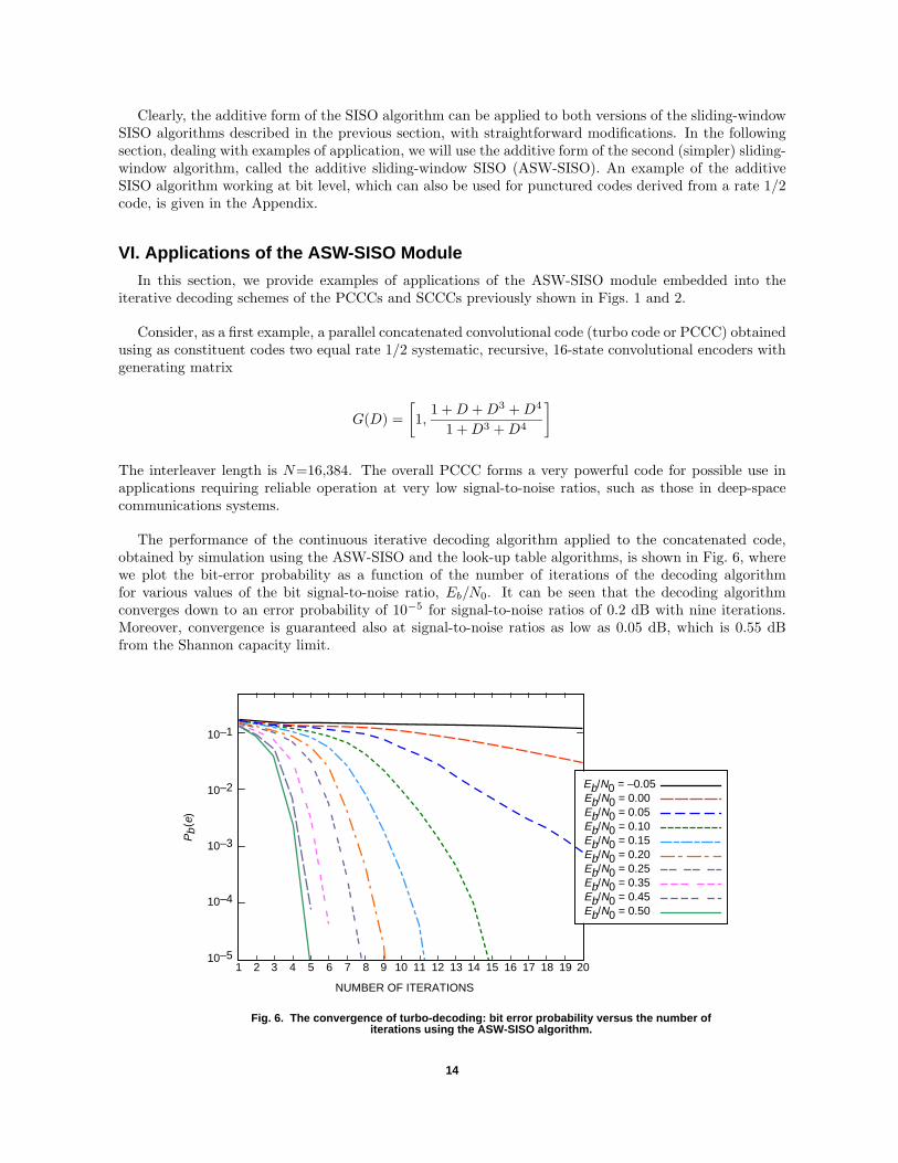
The interleaver length is N=16,384. The overall PCCC forms a very powerful code for possible use inapplications requiring reliable operation at very low signal-to-noise ratios, such as those in deep-spacecommunications systems.

The performance of the continuous iterative decoding algorithm applied to the concatenated code,obtained by simulation using the ASW-SISO and the look-up table algorithms, is shown in Fig. 6, wherewe plot the bit-error probability as a function of the number of iterations of the decoding algorithmfor various values of the bit signal-to-noise ratio, Eb/N0. It can be seen that the decoding algorithmconverges down to an error probability of 10−5 for signal-to-noise ratios of 0.2 dB with nine iterations.Moreover, convergence is guaranteed also at signal-to-noise ratios as low as 0.05 dB, which is 0.55 dBfrom the Shannon capacity limit.

10–1

10–2

10–3

10–4

10–5

Pb

(e)

1 2 3 4 5 6 7 8 9 10 11 12 13 14 15 16 17 18 19 20

NUMBER OF ITERATIONS

Fig. 6. The convergence of turbo-decoding: bit error probability versus the number ofiterations using the ASW-SISO algorithm.

Eb/N0 = –0.05Eb/N0 = 0.00Eb/N0 = 0.05Eb/N0 = 0.10Eb/N0 = 0.15Eb/N0 = 0.20Eb/N0 = 0.25Eb/N0 = 0.35Eb/N0 = 0.45Eb/N0 = 0.50

14

As a second example, we construct the serial concatenation of two convolutional codes (SCCCs) usingas an outer code the rate 1/2, 8-state nonrecursive encoder with generating matrix

G(D) =[1 +D +D3, 1 +D

]and, as an inner code, the rate 1/2, 8-state recursive encoder with generating matrix

G(D) =[1,

1 +D +D3

1 +D

]

The resulting SCCC has rate 1/4. The interleaver length has been chosen to ensure a decoding delay interms of input information bits equal to 16,384.

The performance of the concatenated code, obtained by simulation as before, is shown in Fig. 7, wherewe plot the bit-error probability as a function of the number of iterations of the decoding algorithmfor various values of the bit signal-to-noise ratio, Eb/N0. It can be seen that the decoding algorithmconverges down to an error probability of 10−5 for signal-to-noise ratios of 0.10 dB with nine iterations.Moreover, convergence also is guaranteed at signal-to-noise ratios as low as −0.10 dB, which is 0.71 dBfrom the capacity limit.

Eb/N0 = –0.25Eb/N0 = –0.20Eb/N0 = –0.10Eb/N0 = –0.05Eb/N0 = 0.00Eb/N0 = 0.05Eb/N0 = 0.10

Pb(

e)

1 2 3 4 5 6 7 8 9 10 11 12 13 14 15

NUMBER OF ITERATIONS

Fig. 7. Convergence of iterative decoding for a serial concatenated code: bit error rate probability versus number of iterations using the ASW-SISO algorithm.

10–1

10–2

10–3

10–4

10–5

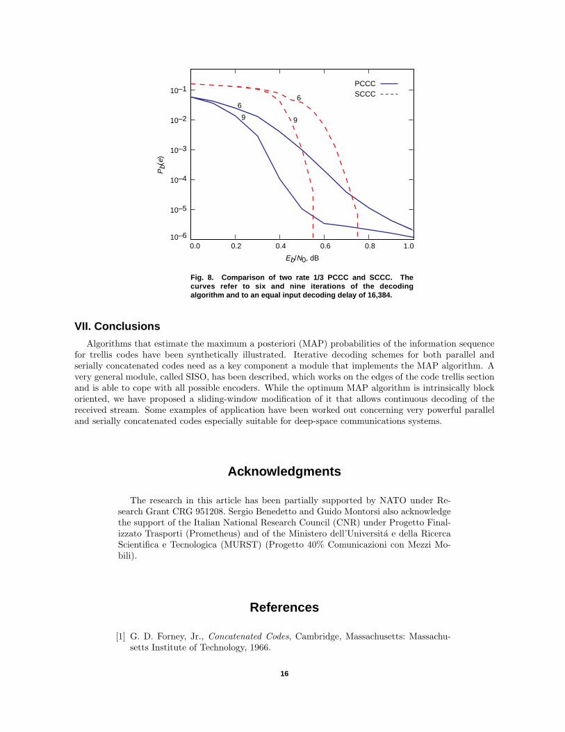
As a third, and final, example, we compare the performance of a PCCC and an SCCC with the samerate and complexity. The concatenated code rate is 1/3, the CCs are four-state recursive encoders (rates1/2 + 1/2 for the PCCCs and rates 1/2 + 2/3 for the SCCCs), and the decoding delays in terms of inputbits are equal to 16,384. In Fig. 8, we report the bit-error probability versus the signal-to-noise ratio forsix and nine decoding iterations. As the curves show, the PCCC outperforms the SCCC for high valuesof the bit-error probabilities. Below 10−5 (for nine iterations), the SCCC behaves significantly betterand does not present the “floor” behavior typical of PCCCs. In particular, at 10−6, the SCCC has anadvantage of 0.5 dB with nine iterations.

15

10–1

10–2

10–3

10–4

10–5

10–60.0 0.2

Eb/N0, dB

Pb(

e)

0.4 0.6 0.8 1.0

PCCC

6

SCCC6

99

Fig. 8. Comparison of two rate 1/3 PCCC and SCCC. The curves refer to six and nine iterations of the decoding algorithm and to an equal input decoding delay of 16,384.

VII. Conclusions

Algorithms that estimate the maximum a posteriori (MAP) probabilities of the information sequencefor trellis codes have been synthetically illustrated. Iterative decoding schemes for both parallel andserially concatenated codes need as a key component a module that implements the MAP algorithm. Avery general module, called SISO, has been described, which works on the edges of the code trellis sectionand is able to cope with all possible encoders. While the optimum MAP algorithm is intrinsically blockoriented, we have proposed a sliding-window modification of it that allows continuous decoding of thereceived stream. Some examples of application have been worked out concerning very powerful paralleland serially concatenated codes especially suitable for deep-space communications systems.

Acknowledgments

The research in this article has been partially supported by NATO under Re-search Grant CRG 951208. Sergio Benedetto and Guido Montorsi also acknowledgethe support of the Italian National Research Council (CNR) under Progetto Final-izzato Trasporti (Prometheus) and of the Ministero dell’Universita e della RicercaScientifica e Tecnologica (MURST) (Progetto 40% Comunicazioni con Mezzi Mo-bili).

References

[1] G. D. Forney, Jr., Concatenated Codes, Cambridge, Massachusetts: Massachu-setts Institute of Technology, 1966.

16

[2] C. Berrou, A. Glavieux, and P. Thitimajshima, “Near Shannon Limit Error-Correcting Coding and Decoding: Turbo-Codes,” Proceedings of ICC’93, Geneva,Switzerland, pp. 1064–1070, May 1993.

[3] S. Benedetto and G. Montorsi, “Iterative Decoding of Serially ConcatenatedConvolutional Codes,” Electronics Letters, vol. 32, no. 13, pp. 1186–1188, June1996.

[4] D. Divsalar and F. Pollara, “Turbo Codes for PCS Applications,” Proceedings ofIEEE ICC’95, Seattle, Washington, pp. 54–59, June 1995.

[5] S. Benedetto, D. Divsalar, G. Montorsi, and F. Pollara, “Serial Concatenationof Interleaved Codes: Performance Analysis, Design, and Iterative Decoding,”The Telecommunications and Data Acquisition Progress Report 42-126, April–June 1996, Jet Propulsion Laboratory, Pasadena, California, pp. 1–26, August15, 1996.http://tda.jpl.nasa.gov/tda/progress report/42-126/126D.pdf

[6] J. Hagenauer, E. Offer, and L. Papke, “Iterative Decoding of Binary Block andConvolutional Codes,” IEEE Transactions on Information Theory, vol. 43, no. 2,pp. 429–445, March 1996.

[7] P. Robertson, “Illuminating the Structure of Decoders for Parallel ConcatenatedRecursive Systematic (Turbo) Codes,” Proceedings of Globecom’94, San Fran-cisco, California, pp. 1298–1303, December 1994.

[8] J. Y. Couleaud, “High Gain Coding Schemes for Space Communications,”ENSICA Final Year Report, University of South Australia, The Levels, Aus-tralia, September 1995.http://www.itr.unisa.edu.au/ steven/turbo/jyc.ps.gz

[9] S. Benedetto, D. Divsalar, G. Montorsi, and F. Pollara, “A Soft-Input Soft-Output MAP Module for Iterative Decoding of Concatenated Codes,” to appearin IEEE Communications Letters, January 1997.

[10] K. Abend and B. D. Fritchman, “Statistical Detection for Communication Chan-nels With Intersymbol Interference,” Proceedings of the IEEE, vol. 58, no, 5,pp. 779–785, May 1970.

[11] R. W. Chang and J. C. Hancock, “On Receiver Structures for Channels HavingMemory,” IEEE Transactions on Information Theory, vol. IT-12, pp. 463–468,October 1966.

[12] L. R. Bahl, J. Cocke, F. Jelinek, and J. Raviv, “Optimal Decoding of LinearCodes for Minimizing Symbol Error Rate,” IEEE Transactions on InformationTheory, vol. 1T-20, pp. 284–287, March 1974.

[13] P. L. McAdam, L. Welch, and C. Weber, “Map Bit Decoding of ConvolutionalCodes,” Abstracts of Papers, ISIT’72, Asilomar, California, p. 91, January 1972.

[14] C. R. Hartmann and L. D. Rudolph, “An Optimum Symbol-by-Symbol DecodingRule for Linear Codes,” IEEE Transactions on Information Theory, vol. IT-22,pp. 514–517, September 1976.

[15] B. Vucetic and Y. Li, “A Survey of Soft-Output Algorithms,” Proceedings ofISITA’94, Sydney, Australia, pp. 863–867 November 1994.

[16] G. D. Forney, Jr., “The Viterbi Algorithm,” IEEE Transactions on InformationTheory, vol. IT-61, no. 3, pp. 268–278, March 1973.

17

[17] H. Yamamoto and K. Itoh, “Viterbi Decoding Algorithm for Convolutional CodesWith Repeat Request,” IEEE Transactions on Information Theory, vol. IT-26,no. 5, pp. 540–547, September 1980.

[18] T. Hashimoto, “A List-Type Reduced-Constraint Generalization of the ViterbiAlgorithm,” IEEE Transactions on Information Theory, vol. IT-33, no. 6,pp. 866–876, November 1987.

[19] R. H. Deng and D. J. Costello, “High Rate Concatenated Coding Systems UsingBandwidth Efficient Trellis Inner Codes,” IEEE Transactions on Communica-tions, vol. COM-37, no. 5, pp. 420—427, May 1989.

[20] N. Seshadri and C-E. W. Sundberg, “Generalized Viterbi Algorithms for ErrorDetection With Convolutional Codes,” Proceedings of GLOBECOM’89, vol. 3,Dallas, Texas, pp. 43.3.1–43.3.5, November 1989.

[21] T. Schaub and J. W. Modestino, “An Erasure Declaring Viterbi Decoder and ItsApplications to Concatenated Coding Systems,” Proceedings of ICC’86, Toronto,Canada, pp. 1612–1616, June 1986,.

[22] J. Hagenauer and P. Hoeher, “A Viterbi Algorithm With Soft-Decision Outputsand Its Applications,” Proceedings of GLOBECOM’89, Dallas, Texas, pp. 47.1.1–47.1.7, November 1989.

[23] P. Hoeher, “TCM on Frequency-Selective Fading Channels: A Comparisonof Soft-Output Probabilistic Equalizers,” Proceedings of GLOBECOM’90, SanDiego, California, pp. 40l.4.l–40l.4.6, December 1990.

[24] U. Hansson, “Theoretical Treatment of ML Sequence Detection With a Con-catenated Receiver,” Technical Report 185L, School of Electrical and ComputerEngineering, Chalmers University of Technology, Goteborg, Sweden, 1994.

[25] S. S. Pietrobon and A. S. Barbulescu, “A Simplification of the Modified Bahl Al-gorithm for Systematic Convolutional Codes,” Proceedings of ISITA’94, Sydney,Australia, pp. 1073–1077, November 1994.

[26] P. Robertson, E. Villebrun, and P. Hoeher, “A Comparison of Optimal and Sub-Optimal MAP Decoding Algorithms Operating in the Log Domain,” Proceedingsof ICC’95, Seattle, Washington, pp. 1009–1013, June 1995.

[27] P. Jung, “Novel Low Complexity Decoder for Turbo Codes,” Electronics Letters,vol. 31, no. 2, pp. 86–87, January 1995.

[28] S. Benedetto, D. Divsalar, G. Montorsi, and F. Pollara, “Algorithm for Contin-uous Decoding of Turbo Codes,” Electronics Letters, vol. 32, no. 4, pp. 314–315,February 1996.

[29] L. Papke, P. Robertson, and E. Villebrum, “Improved Decoding With the SOVAin a Parallel Concatenated (Turbo-Code) Scheme,” Proceedings of IEEE ICC’96,Dallas, Texas, pp. 102–106, June 1996.

[30] S. Benedetto, D. Divsalar, G. Montorsi, and F. Pollara, “Soft-Output Decod-ing Algorithms for Continuous Decoding of Parallel Concatenated ConvolutionalCodes,” Proceedings of IEEE ICC’96, Dallas, Texas, pp. 112–117, June 1996.

[31] S. Benedetto, D. Divsalar, G. Montorsi, and F. Pollara, “Soft-Output DecodingAlgorithms in Iterative Decoding of Turbo Codes,” The Telecommunications andData Acquisition Progress Report 42-124, October–December 1995, Jet Propul-sion Laboratory, Pasadena, California, pp. 63–87, February 15, 1996.http://tda.jpl.nasa.gov/tda/progress report/42-124/124G.pdf

18

Appendix

An Example of the Additive SISO Algorithm Working at Bit Level

This appendix describes the SISO algorithm used in the example of serial concatenation of two rate1/2 convolutional codes. Consider a rate 1/2 convolutional code. Let Uk be the input bit and C1,k andC2,k the output bits of the convolutional code at time k, taking values {0, 1}. Therefore, on the trellisedges at time k we have uk(e), c1,k(e), c2,k(e). In the following, for simplicity of notation, we drop thesubscript k for the input and output bits. Define the reliability of a bit Z taking values {0, 1} at time kas

λk[Z; ·] 4= logPk[Z = 1; ·]Pk[Z = 0; ·] = πk[Z = 1; ·]− πk[Z = 0; ·]

The second argument in the brackets, shown by a dot, may represent I, the input, or O, the output, tothe SISO. We use the following identity:

a = log

[L∑i=1

eai

]= max

i{ai}+ δ(a1, . . . , aL) 4= max

i

∗{ai}

where δ(a1, . . . , aL) is the correction term, as discussed in Section V, that can be computed using alook-up table. We defined the “max∗” operation as a maximization (compare–select) plus a correctionterm (look-up table). Using the results of Sections III.D, IV, and V, we obtain the forward and thebackward recursions as

αk(s) = max∗e:sE(e)=s

{αk−1

[sS(e)

]+ u(e)λk[U ; I] + c1(e)λk[C1; I] + c2(e)λk[C2; I]}+ hαk

βk(s) = max∗e:sS(e)=s

{βk+1

[sE(e)

]+ u(e)λk+1[U ; I] + c1(e)λk+1[C1; I] + c2(e)λk+1[C2; I]}+ hβk

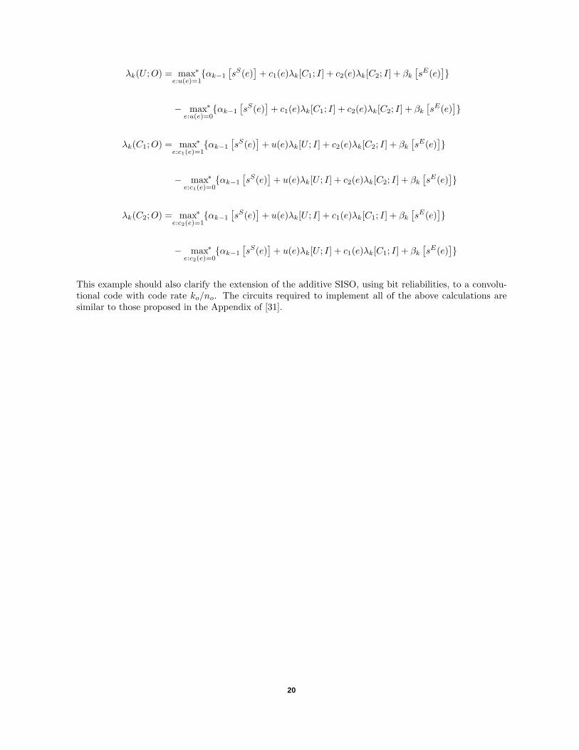
with initial values α0(s) = 0 if s = S0, and α0(s) = −∞ otherwise, and βn(s) = 0 if s = Sn, and βn(s)= −∞ otherwise, where hαk and hβk are normalization constants, which, for a hardware implementationof the SISO, are used to prevent buffer overflow. These operations are similar to those employed by theViterbi algorithm when it is used in the forward and backward directions, except for a correction termthat is added when compare–select operations are performed.

For the inner decoder, which is connected to the AWGN channel, we have λk[C1; I] = (2A/σ2)r1,k andλk[C2; I] = (2A/σ2)r2,k, where ri,k = A(2ci − 1) + ni,k, i = 1, 2, is the received samples at the outputof the receiver matched filter, ci ∈ {0, 1}, and ni,k is the zero-mean independent identically distributed(i.i.d.) Gaussian noise samples with variance σ2.

The extrinsic bit information for U , C1, and C2 can be obtained as

19

λk(U ;O) = maxe:u(e)=1

∗ {αk−1

[sS(e)

]+ c1(e)λk[C1; I] + c2(e)λk[C2; I] + βk

[sE(e)

]}

− maxe:u(e)=0

∗ {αk−1

[sS(e)

]+ c1(e)λk[C1; I] + c2(e)λk[C2; I] + βk

[sE(e)

]}

λk(C1;O) = maxe:c1(e)=1

∗ {αk−1

[sS(e)

]+ u(e)λk[U ; I] + c2(e)λk[C2; I] + βk

[sE(e)

]}

− maxe:c1(e)=0

∗ {αk−1

[sS(e)

]+ u(e)λk[U ; I] + c2(e)λk[C2; I] + βk

[sE(e)

]}

λk(C2;O) = maxe:c2(e)=1

∗ {αk−1

[sS(e)

]+ u(e)λk[U ; I] + c1(e)λk[C1; I] + βk

[sE(e)

]}

− maxe:c2(e)=0

∗ {αk−1

[sS(e)

]+ u(e)λk[U ; I] + c1(e)λk[C1; I] + βk

[sE(e)

]}

This example should also clarify the extension of the additive SISO, using bit reliabilities, to a convolu-tional code with code rate ko/no. The circuits required to implement all of the above calculations aresimilar to those proposed in the Appendix of [31].

20