I hereby declare that I am the sole author of this thesis. This is a true copy of the thesis, including any
required final revisions, as accepted by my examiners.
I understand that my thesis may be made electronically available to the public.
iii
Abstract
Face recognition, as one of the major biometrics identification methods, has been applied in different
fields involving economics, military, e-commerce, and security. Its touchless identification process and
non-compulsory rule to users are irreplacable by other approaches, such as iris recognition or fingerprint
recognition. Among all face recognition techniques, principal component anaylsis (PCA) was proposed in
the earliest stage; however, it is still attracting researchers in this field because of its property of reducing
data dimensionality without losing important information.
PCA-based face recognition has been studied for decades. There exist some image processing toolkits
like OpenCV, which have implemented the PCA algorithm and associated methods. Nevertheless,
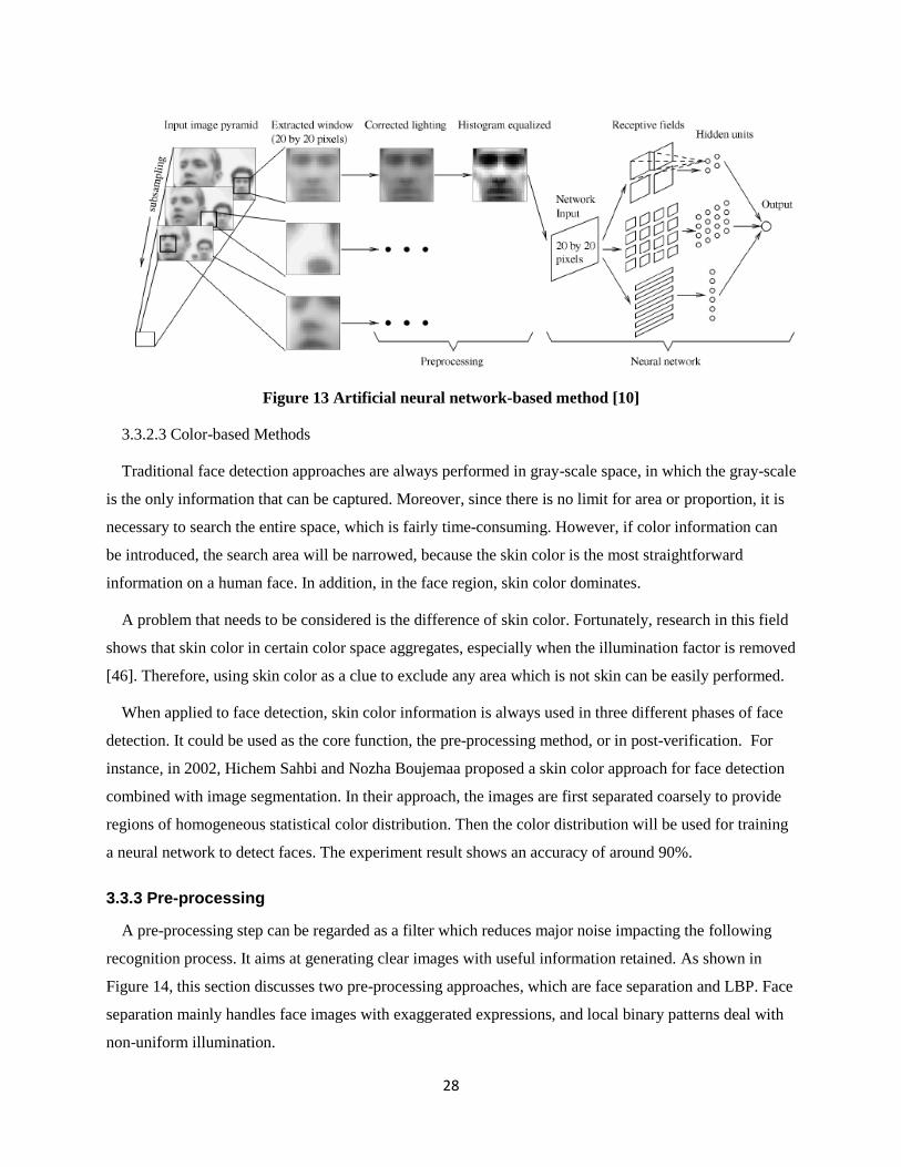
establishing a PCA-based face recognition system is still time-consuming, since there are different
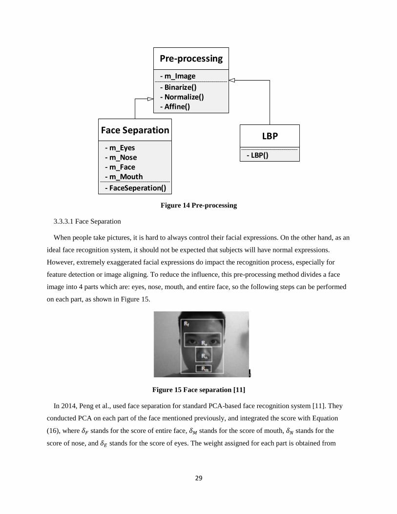
problems that need to be considered in practical applications, such as illumination, facial expression, or
shooting angle, which can hardly be solved by the toolkits. Furthermore, it still costs a lot of effort for
software developers to integrate the implementations of the toolkits with their own applications.
Therefore, the thesis provides a software framework for PCA-based face recognition aimed at assisting
software developers to customize their applications efficiently. The framework describes the complete
process of PCA-based face recognition, and in each step, multiple variations are offered for different
requirements. Through various combination of these variations, at least 108 variations can be produced by
the framework. Moreover, some of the variations in the same step can work collaboratively and some
steps can be omitted in specific situations; thus, the total number of variations exceeds 150. The
implementation of all approaches presented in the framework is provided.
iv
Acknowledgements
I would like to thank Professor Paulo Alencar, for his kindness, understanding and guidance. It has been
my honor to be his student and I learned a lot while working with him. I’m very grateful to Professor
Daniel Berry for serving as my co-supervisor. Thanks to Professor Donald Cowan for helping me revise
my paper and thesis. I also thank Professor Donald Cowan and Professor Ladan Tahvildari for agreeing to
read my thesis and providing me valuable feedback.
Immense gratitude towards my parents Zhenyun and Hongwei for their unconditional love.
Special thanks to my girlfriend Amy for her constant care and love.
Finally, thanks to my friends Akshat Kumar and Vishnu Srivastava for sharing their wisdom.
v
Dedication
Dedicated to my uncle Xiaohua Peng
vi
Table of Contents
AUTHOR'S DECLARATION .................................................................................................................... ii
Abstract ..................................................................................................................................................... iii
Acknowledgements ................................................................................................................................ iv
Dedication .................................................................................................................................................. v
List of Figures .......................................................................................................................................... ix
1.1 Related Areas ...................................................................................................................................... 2
1.1.1 Face Recognition System ................................................................................................................. 2
1.1.2 Principal Component Analysis.......................................................................................................... 3
1.2 Problem ............................................................................................................................................... 5
Related Work ............................................................................................................................................. 7
2.1 Face Recognition Framework .............................................................................................................. 7
2.1.1 Face detection .................................................................................................................................. 7
2.1.2 Face Recognition .............................................................................................................................. 8
2.2 Principal Component Analysis ............................................................................................................. 9
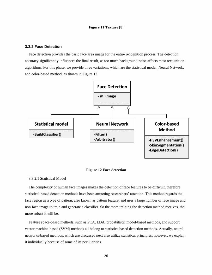
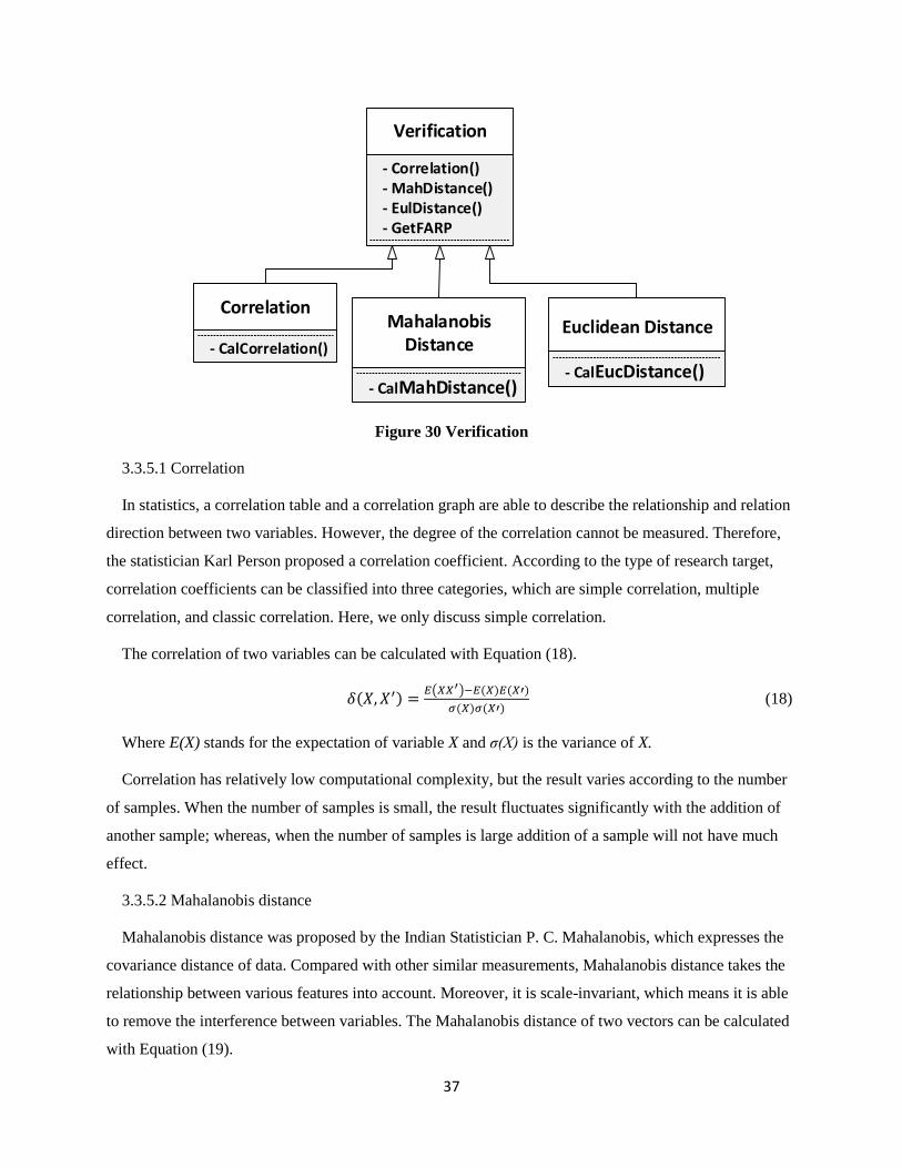
3.2.2 Face Detection ............................................................................................................................... 16
3.3.2 Face Detection ............................................................................................................................... 26
4.1.4 Face Detection ............................................................................................................................... 42
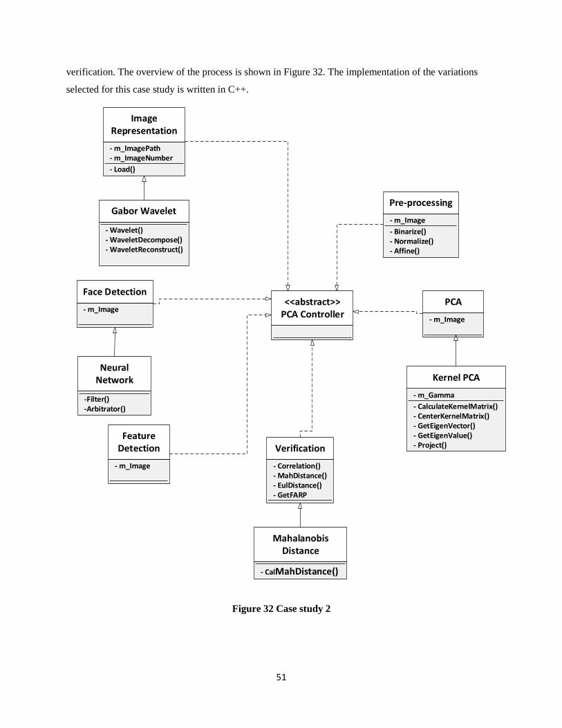
4.2 Case study 2 ...................................................................................................................................... 50
4.2.2 Face Representation ...................................................................................................................... 52
4.2.3 Face Detection ............................................................................................................................... 59
4.3 Other Case Studies ............................................................................................................................ 67
4.3.1 Case Study 3 ................................................................................................................................... 67
4.3.2 Case Study 4 ................................................................................................................................... 70
5.2 Future work ....................................................................................................................................... 74
Figure 22 Original dataset [39] ................................................................................................................... 33
Figure 23 Eigenvalues and eigenvectors [39] ............................................................................................. 33
Figure 24 Classification by using standard PCA [39] ................................................................................... 34
Figure 25 Data type [39] ............................................................................................................................. 34
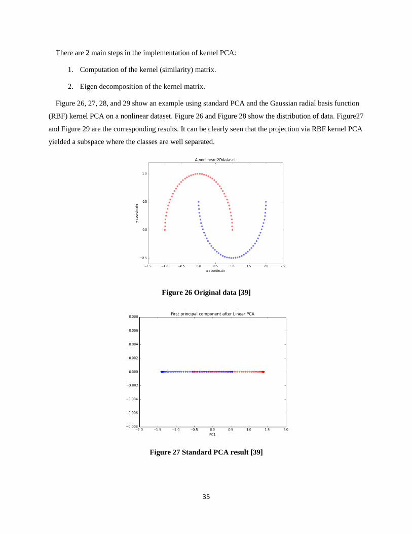
Figure 26 Original data [39] ........................................................................................................................ 35
Figure 27 Standard PCA result [39] ............................................................................................................. 35
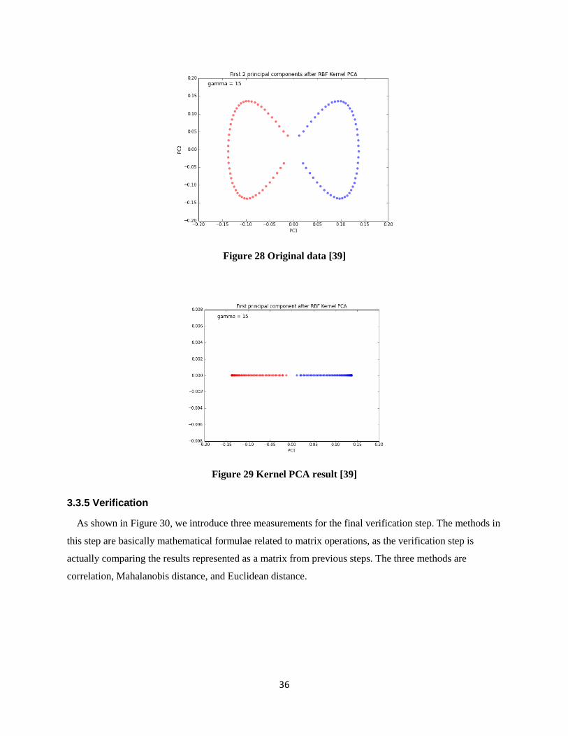
Figure 28 Original data [39] ........................................................................................................................ 36
Figure 29 Kernel PCA result [39] ................................................................................................................. 36
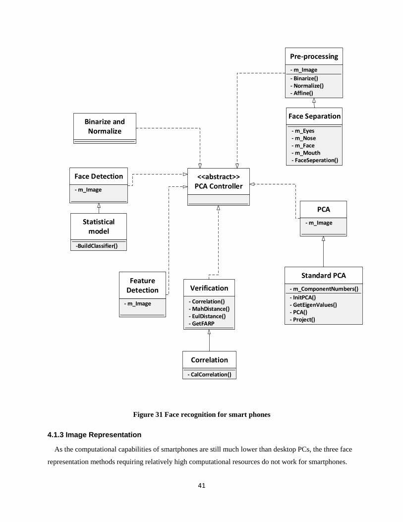
Figure 31 Face recognition for smart phones ............................................................................................. 41
Figure 32 Case study 2 ................................................................................................................................ 51
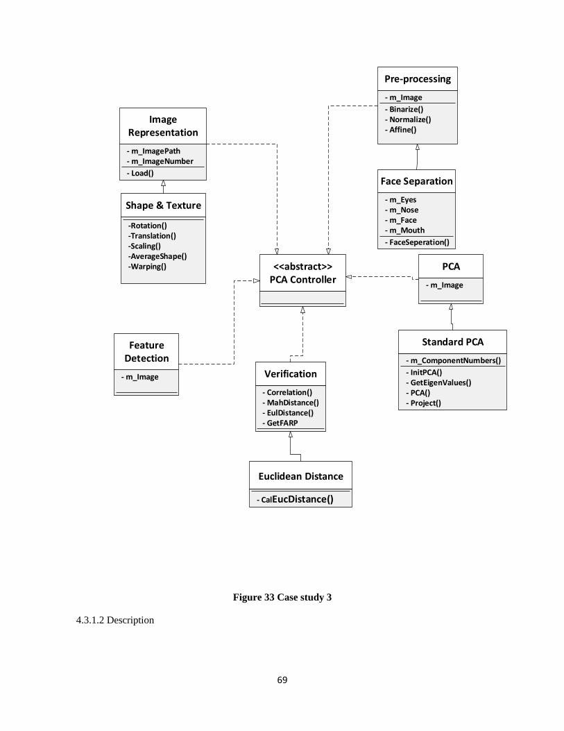
Figure 33 Case study 3 ................................................................................................................................ 69
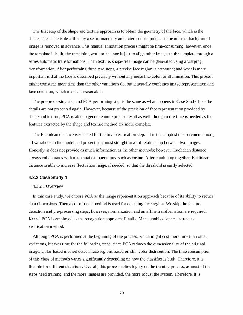
Figure 34 Case study 4 ................................................................................................................................ 71
1
Chapter 1
Introduction
Face recognition has been studied for decades and has been applied in various areas. In 2012, Samsung
released their new smart TV which incorporates face recognition by using built-in camera. This new
feature allows users to log in to social network applications, such as Facebook, Twitter, or Skype without
resorting to a userid and password. In addition, face recognition has also attracted the attention of
governments because of its high security level and accessibility. DARPA (Defense Advanced Research
Projects Agency) intends to supplant traditional digital passwords by scanning human faces [1]. Face
recognition techniques even can support law enforcement. Karl Ricanek Jr. introduced an application of
face recognition in detecting potential child pornography in computer storage. The results show
significant progress in both detection speed and accuracy [2].
Recognizing human faces with computers originates from research in 1964, by Helen Chan and Charles
Bisson [3]. Initially, most research focused on detecting individual features, such as eyes, nose, and
mouth. As mathematical approaches developed, researchers focused their attention on describing the
entire face with statistical methods, which led to further advances in face recognition. Currently, face
recognition methods can be classified into categories such as feature-based recognition, appearance-based
recognition, template-based recognition, etc. However, principal component analysis (PCA), as proposed
by Alex P. Pentland in 1991 [4] is still one of the most popular analysis techniques. A number of
variations based on the standard PCA approach have been developed for different situations. The PCA
property of reducing data dimensionality without losing principal components is the key feature that
makes it an object of continuing study.
Although PCA is a mature technique, it is still time-consuming to implement the algorithm, especially
when adapting it to different types of data, or combining it with pre-processing and result generation
steps. Some popular image processing toolkits, such as OpenCV, have standard PCA algorithms, but
these libraries are not designed to help users customize applications. Furthermore, the multiple variations
of PCA also need to be considered, since they produce better results when being used under extreme
situations, such as non-uniform illumination, or exaggerated facial expressions. Additionally, associated
steps such as face detection and pre-processing also play an important role in terms of the entire face
recognition process. Selecting appropriate approaches in each step according to specific situations
positively affects the final recognition accuracy.
2
This thesis intends to propose a software framework for PCA-based face recognition aiming at assisting
software developers to customize their own applications efficiently. The framework describes the
complete process of PCA-based face recognition, and in each step, multiple variations are offered for
different requirements. Through different combinations of these variations, at least 108 variations can be
produced by the framework. Moreover, some of the variations in the same step can work collaboratively
and some steps can be omitted in specific situations; thus, the total of variations exceeds 150. The
implementation of all approaches in the framework is provided.
With the framework, software developers working on face recognition applications are able to build
their applications quickly through software reuse, as the task becomes a design process at a higher level.
After clarifying the requirements of the applications, the framework helps developers to select appropriate
variations for each step in the face recognition system. As the framework describes the entire PCA-based
face recognition process and demonstrates what type of situations are dealt by the variations, developers
simply choose a variation for each step according to the guide of the framework and then build their
application.
As an example, if the developer intends to build a face recognition application used for security which
works on a high performance computer, the framework will prioritise the recognition accuracy, whereas
the responding speed becomes to a minor factor, since the high performance computer is able to provide
enough computation resources. However, when the face recognition is used for smart phones, providing
real-time feedback to users is more important, and some extreme environmental conditions such as non-
uniform illumination need to be considered. Thus, the framework provides variations which generate
results fast and can deal with different working environments.
The thesis presents four case studies based on the variations produced by the framework. The first case
study is a face recognition system for smart phones. The other three case studies aim to cover all
variations to give a comprehensive impression of the framework to readers. For instance, the Case Study
2 describes a face recognition application working on high performance computers. However, the
possible applications which can be produced by the framework are not limited to the case studies.
1.1 Related Areas
1.1.1 Face Recognition System
Currently, personal identification still heavily relies on traditional password encryption. This method
do help people protect their privacy; however, with the development of other high-tech fields, the security
level provided by a password is not able to meet our requirements, as it is based on “what the person
possesses” and “what the person remembers”, instead of “who the person is”. Fortunately, a new research
3
area, biometric recognition, offers a number of technical methods, which may make truly reliable
personal identification come true.
In the field of biometrics recognition, face recognition is the friendliest, most direct and natural
method. Compared with other recognition approaches, such as fingerprint recognition or iris recognition,
face recognition does not invade personal privacy or disturb people. Additionally, a face image is easier to
capture, even without making the person aware that an image is being made.
According to a report from The 3rd China Guangzhou International Biometric Identification
Technology Expo in 2016, the total revenue of global biometric identification market reached 9.368 billon
USD in 2014. Face recognition had a market share of 11.4%, the largest percentage of revenue among all
the identification approaches [19].
Generally, an automatic face recognition system is divided into phases, face detection and face
recognition. In the face detection stage, the face area is extracted from the background image, and the size
of the area is also defined at the same time. In the face recognition stage, the face image will be
represented with mathematical approaches to express as much information about the face as possible.
Eventually, the new face image will be compared with known face images, which results in a similarity
score for final verification.
Thanks to a human being’s eyes, the aforementioned two phases can be easily completed. However,
building an automatic face recognition system with high accuracy is challenging, as every phase in the
recognition process is susceptible to internal physiological and external environmental factors. Therefore,
face recognition is still attracting researchers.
1.1.2 Principal Component Analysis
The earliest principal component analysis dates back to 1901 when Karl Pearson proposed the concept
and applied it to non-random variables [6]. In 1930, Harold Hotelling extended it to random variables [17]
[18]. The technique is now being applied in a number of fields, such as mechanics, economics, medicine,
and neuroscience. In computer science, PCA is utilized as a data dimensionality reduction tool. Especially
in the age of Big Data, the data we process is often complex and huge. So reducing the computational
complexity and saving computing resources are important issues.
Basically, the PCA process projects the original data with high dimensionality to a lower
dimensionality subspace through a linear transformation. Nevertheless, the projection is not arbitrary. It
has to obey a rule that the most representative data needs to be retained, i.e. the data after transforming
cannot be distorted. Hence, those dimensionalities which are reduced by PCA are actually redundant or
even noisy. Therefore, the ultimate goal of conducting PCA is to refine data so that the noisy and
4
redundant part can be removed and only the useful part is retained. It is because of this feature that PCA
is widely used in face recognition. Images are represented as a high dimensional matrix in computers, and
removing noise from images is a necessary pre-processing step.
1.1.3 Object-oriented Framework
An object-oriented framework is a group of correlated classes for a specific domain of software. It
defines the architecture of a class of user applications, the separation of object and class, the functionality
of each part, how the object and class collaborate, and the controlling process. Therefore, one focus of an
object-oriented framework is software reusability [58].
Software reuse uses existing knowledge of a software to build a new software, so that to reduce the cost
of development and maintainence. In 1992, Charles W. Krueger suggested five dimensions for a good
software reuse, which are abstraction and classification in terms of building for software reuse process,
and selection, specialization and integration in terms of building with software reuse process. Abstraction
and classification means that in software reuse, the reusable knowledge should be represented concisely
and classified. Selection, specialization and integration indicate that reusable knowledge should be
parameterized for query, specialized for new situations, and integrated for customer projects [59].
A framework can be viewed as the combination of abstract class and concrete class. The abstract class
is defined in the framework, whereas the concrete class is implemented in the application. Simply, a
framework is the outline of an application, which contains the common objects for a specific domain. In
addition, a framework includes some design parameters, which can be used as interfaces, to be applied to
different applications.
1.1.4 Machine Learning Approaches
Machine learning is an interdisciplinary subject consisting of many different areas, such as probability,
statistics, approximation theory, and algorithm theory. Arthur Samuel first defined machine learning as a
“Field of study that gives computers the ability to learn without being explicitly programmed” [3].
Machine learning focuses on simulating human beings’ behaviors to gain new knowledge and skills
with a computer. Furthermore, it is able to recombine the learned knowledge and keep improving its
performance.
Typically, machine learning is classified into three categories, which are supervised learning,
unsupervised learning, and reinforcement learning [20]. The difference mainly depends on whether the
computer is taught or not. In supervised learning, the computer is given input along with its
corresponding output. However, in unsupervised learning, no labels are provided, so the computer needs
5
to learn on its own. Unsupervised learning does not always have an explicit goal, which means that it is
allowed to find a goal by itself. Reinforcement learning can be treated as a compromise between the two
aforementioned approaches. It has an explicit goal, but it needs to interact in a dynamic environment in
which no teaching is provided.
1.2 Problem
Although there exists a number of image processing toolkits like OpenCV, which have PCA algorithm
as well as associated approaches for face recognition, it is still time-consuming for software developers
who intend to integrate face recognition implementations with their own applications. Furthermore,
selecting appropriate approaches for each step in the process of face recognition is non-trivial, since it
directly impacts the final recognition result. For face recognition systems which run under extreme
situations, such as non-uniform illumination, exaggerated facial expression, or facial region occlusion,
approach selection becomes even more significant. In fact, building a PCA-based face recognition system
should not cost a lot of effort for developers, as the technique has been studied for years and is mature.
The time spent on implementing the algorithms and integrating with their applications should not be
necessary.
1.3 Proposed Approach
This thesis provides a software framework for PCA-based face recognition aiming at assisting software
developers to customize their own applications efficiently. The framework describes the complete process
of PCA-based face recognition including image representation, face detection, feature detection, pre-
processing, PCA, and verification, and in each step, multiple variations are offered to fit different
requirements. Through various combinations of these variations, at least 108 variations can be generated
by the framework. Moreover, some of the variations in the same step can work collaboratively and some
steps can be omitted in specific situations; thus, the total number of variations exceeds 150. The
implementation of all approaches presented in the framework is provided. As the framework strictly
follows the normal process of PCA-based face recognition, it can be easily extended, which means more
approaches are able to be attached to any of the steps.
1.4 Evaluations
In the thesis we present a framework followed by four case studies. The first case study is for face
recognition using on smart phones. The other three case studies cover almost every variation supported by
the framework.
6
1.5 Contributions
The main contributions described in this thesis are:
1. A model which includes the entire facial recognition process using PCA with multiple
variations in each phase for different facial conditions;
2. A high-level framework design;
3. Implementation of the framework; and
4. A support tool for facial recognition with PCA
1.6 Thesis Outline
Chapter 2 presents work related to the research which mainly includes four sections. The first section
introduces general requirements of face recognition system. The second section focuses on principal
component analysis which is the core algorithm of this research. The third section explains the concept of
object-oriented frameworks. The last section talks about machine learning. Chapter 3 demonstrates the
framework. Chapter 4 describes the case studies based on the proposed framework. Chapter 5 concludes
the thesis and suggests future work.
7
Chapter 2
Related Work
As mentioned in Chapter 1, this chapter introduces work in four areas related to our research. First, a
classical face recognition framework is demonstrated. Then, we present a brief introduction to principal
component anaylsis (PCA) describing the history of the approach, the mathematical principal behind
PCA, and its development in face recognition. Third, object-oriented frameworks are discussed. Last, we
investigate machine learning approaches, since its outstanding classifying ability has been attracting
researchers in face recognition.
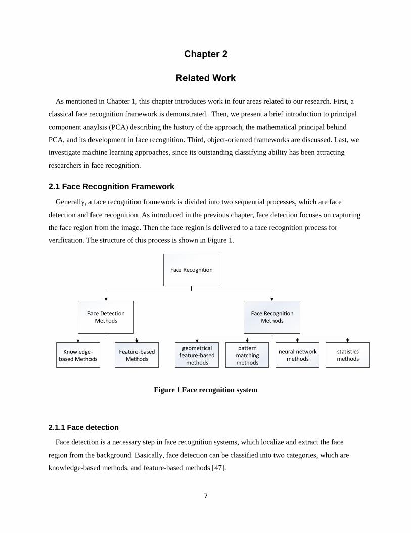
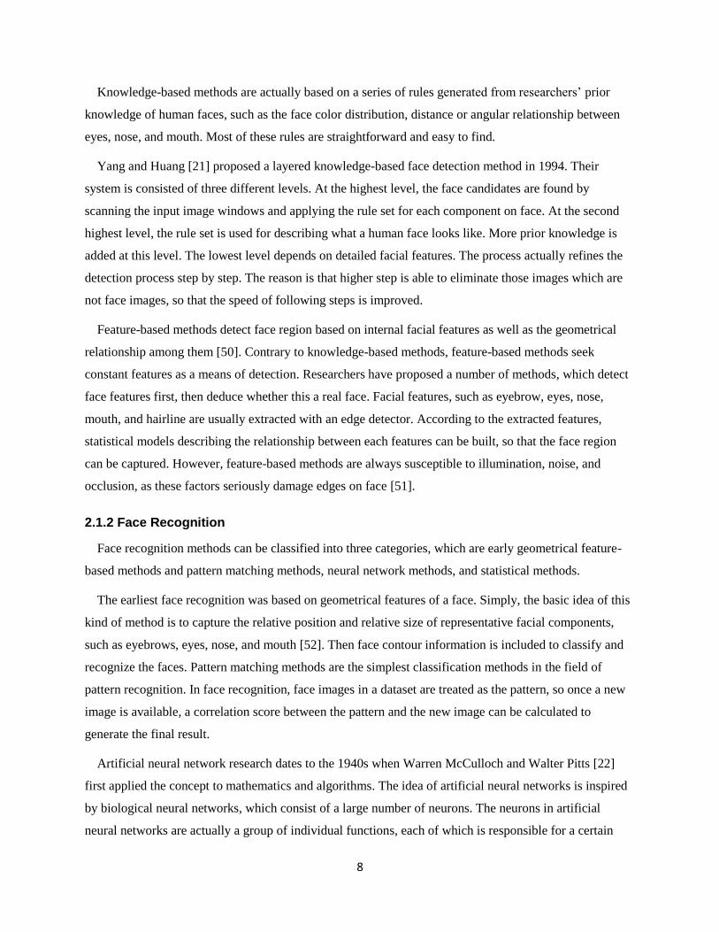
2.1 Face Recognition Framework
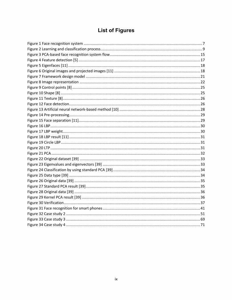
Generally, a face recognition framework is divided into two sequential processes, which are face
detection and face recognition. As introduced in the previous chapter, face detection focuses on capturing
the face region from the image. Then the face region is delivered to a face recognition process for
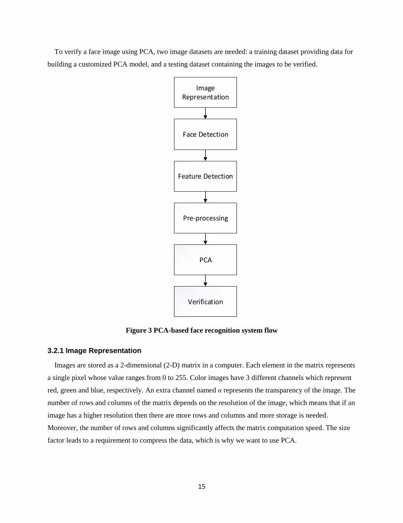
verification. The structure of this process is shown in Figure 1.
Face Recognition
Face Detection Methods
Face Recognition Methods
Knowledge-based Methods
Feature-based Methods
geometrical feature-based
methods
pattern matching methods
neural network methods
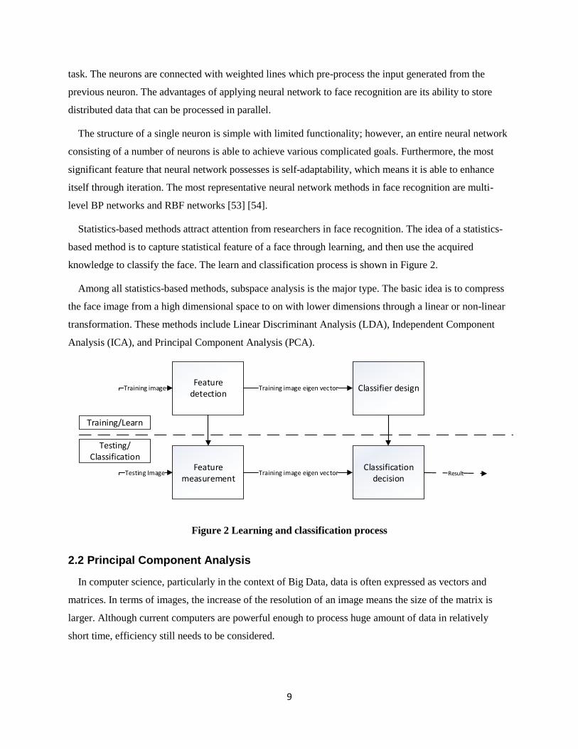
statistics methods
Figure 1 Face recognition system
2.1.1 Face detection
Face detection is a necessary step in face recognition systems, which localize and extract the face
region from the background. Basically, face detection can be classified into two categories, which are
knowledge-based methods, and feature-based methods [47].
8
Knowledge-based methods are actually based on a series of rules generated from researchers’ prior
knowledge of human faces, such as the face color distribution, distance or angular relationship between
eyes, nose, and mouth. Most of these rules are straightforward and easy to find.
Yang and Huang [21] proposed a layered knowledge-based face detection method in 1994. Their
system is consisted of three different levels. At the highest level, the face candidates are found by
scanning the input image windows and applying the rule set for each component on face. At the second
highest level, the rule set is used for describing what a human face looks like. More prior knowledge is
added at this level. The lowest level depends on detailed facial features. The process actually refines the
detection process step by step. The reason is that higher step is able to eliminate those images which are
not face images, so that the speed of following steps is improved.
Feature-based methods detect face region based on internal facial features as well as the geometrical
relationship among them [50]. Contrary to knowledge-based methods, feature-based methods seek
constant features as a means of detection. Researchers have proposed a number of methods, which detect
face features first, then deduce whether this a real face. Facial features, such as eyebrow, eyes, nose,
mouth, and hairline are usually extracted with an edge detector. According to the extracted features,
statistical models describing the relationship between each features can be built, so that the face region
can be captured. However, feature-based methods are always susceptible to illumination, noise, and
occlusion, as these factors seriously damage edges on face [51].
2.1.2 Face Recognition
Face recognition methods can be classified into three categories, which are early geometrical feature-
based methods and pattern matching methods, neural network methods, and statistical methods.
The earliest face recognition was based on geometrical features of a face. Simply, the basic idea of this
kind of method is to capture the relative position and relative size of representative facial components,
such as eyebrows, eyes, nose, and mouth [52]. Then face contour information is included to classify and
recognize the faces. Pattern matching methods are the simplest classification methods in the field of
pattern recognition. In face recognition, face images in a dataset are treated as the pattern, so once a new
image is available, a correlation score between the pattern and the new image can be calculated to
generate the final result.
Artificial neural network research dates to the 1940s when Warren McCulloch and Walter Pitts [22]
first applied the concept to mathematics and algorithms. The idea of artificial neural networks is inspired
by biological neural networks, which consist of a large number of neurons. The neurons in artificial
neural networks are actually a group of individual functions, each of which is responsible for a certain
CPCAAlgoritm::CPCAAlgoritm(int iImgWidth, int iImgHeight, int iNumSamples, PBYTE pbyImgSamples) : CLinear2DArray(iImgWidth * iImgHeight, iNumSamples, sizeof(float)), m_iImgWidth(iImgWidth), m_iImgHeight(iImgHeight), m_iImgSize(iImgWidth * iImgHeight), m_iNumSamples(iNumSamples), m_pbyImgSamples(pbyImgSamples), m_pPCAModel(NULL) { ASSERT(m_iImgSize > m_iNumSamples); } BOOL CPCAAlgoritm::GetPCAModel(CPCAModel *pPCAModel) { float fPrecision = (float)0.001, *pfAllEigenVectors, *pfTempCovarianceArray; int iIterationTime = 100; DWORD dwFullSize = m_iNumSamples * m_iNumSamples; //allocate memory for the model pPCAModel->SetDimensions(m_iImgWidth, m_iImgHeight, m_iNumSamples); //allocate temp memory pfTempCovarianceArray = new float[dwFullSize]; pfAllEigenVectors = new float[dwFullSize]; //find the mean vector and the covariance array CalculateCovariance(pPCAModel->MeanImgVector(), pPCAModel->CovarianceArray()); //get all eigen vectors from the covariance array memcpy(pfTempCovarianceArray, pPCAModel->CovarianceArray(), sizeof(float) * dwFullSize); //reserve the original covariance array ::MatrixEigenVectors(pfTempCovarianceArray, m_iNumSamples, pfAllEigenVectors, fPrecision, iIterationTime); //get low-dimensional eigen values and vectors int iNumEigenVectors = CalcalateNewSD(pfTempCovarianceArray, pfAllEigenVectors, pPCAModel); // pPCAModel->SetNumEigens(iNumEigenVectors); delete []pfAllEigenVectors; delete []pfTempCovarianceArray; return TRUE; } //end of CPCAAlgoritm::DoPCA() void CPCAAlgoritm::CalculateCovariance(PFLOAT pfMeanImgVector, PFLOAT pfCovarianceArray)
85
{ int i, j, k; float dTmp; // pfMeanImgVector[], row by row for (j = 0; j < m_iImgSize; j++){ dTmp = 0.0; for (i = 0; i < m_iNumSamples; i++) dTmp += (float)m_pbyImgSamples[m_pRows[i] + j]; pfMeanImgVector[j] = dTmp / m_iNumSamples; } // m_iNumSamples * m_iNumSamples for (i = 0; i < m_iNumSamples; i++){ //row by row for (j = 0; j <= i; j ++){ //colum by colum dTmp = 0.0; for (k = 0; k < m_iImgSize; k++) dTmp += ((float)m_pbyImgSamples[m_pRows[i] + k] - pfMeanImgVector[k]) * ((float)m_pbyImgSamples[m_pRows[j] + k] - pfMeanImgVector[k]); //dTmp += (float)(m_pbyImgSamples[i][k]) * (float)(m_pbyImgSamples[j][k]); pfCovarianceArray[m_pCols[i] + j] = dTmp / m_iImgSize; } } //pfCovarianceArray for (i = 0; i < m_iNumSamples; i++){ for (j = i + 1; j < m_iNumSamples; j++) pfCovarianceArray[m_pCols[i] + j] = pfCovarianceArray[m_pCols[j] + i]; } } //end of CPCAAlgoritm::CalculateCovariance() int CPCAAlgoritm::CalcalateNewSD(PFLOAT pfCovarianceArray, PFLOAT pfAllEigenVectors, CPCAModel *pPCAModel) { DWORD dwFullDataSize = m_iNumSamples * m_iNumSamples; float dTmp, pfEigenValuesSum, dValve; int i, j, k, iNumEigenVectors; PFLOAT pfAllEigenValues = new float[m_iNumSamples * 2]; PFLOAT pfResultTmp = new float[dwFullDataSize]; PFLOAT pfEigenValueArray = new float[dwFullDataSize]; PFLOAT pfTmpEigenVectors = new float[dwFullDataSize]; for (i = 0; i < (int)dwFullDataSize; i++) pfEigenValueArray[i] = pfTmpEigenVectors[i] = 0.0; for (i = 0; i < m_iNumSamples; i++){ pfAllEigenValues[i + i] = pfCovarianceArray[m_pCols[i] + i]; //value pfAllEigenValues[i + i + 1] = float(i); //index } ::BubbleSortFloat(pfAllEigenValues, m_iNumSamples, m_iNumSamples); pfEigenValuesSum = 0.0; for (i = 0; i < 2 * m_iNumSamples; i += 2) pfEigenValuesSum += pfAllEigenValues[i];
86
iNumEigenVectors = 0; dTmp = 0.0; dValve = (float)0.95; for (i = 0; i < m_iNumSamples; i++){ dTmp += pfAllEigenValues[i + i] / pfEigenValuesSum; if (dTmp >= dValve){ iNumEigenVectors = i + 1; break; } } //set number of eigens and allocate memory pPCAModel->SetNumEigens(iNumEigenVectors); // for (i = 0; i < iNumEigenVectors; i++) pPCAModel->EigenValues()[i] = pfAllEigenValues[i << 1]; // (m_iNumSamples * iNumEigenVectors) for (i = 0; i < iNumEigenVectors; i++){ pfEigenValueArray[m_pCols[i] + i] = float(1.0 / sqrt (pfAllEigenValues[i << 1])); k = (int)pfAllEigenValues[i + i + 1]; for (j = 0; j < m_iNumSamples; j++) pfTmpEigenVectors[m_pCols[j] + i] = pfAllEigenVectors[m_pCols[j] + k]; } // (iNumEigenVectors * m_iNumSamples) for (i = 0; i < m_iNumSamples; i++){ for (j = 0; j <= i - 1; j++){ dTmp = pfTmpEigenVectors[m_pCols[i] + j]; pfTmpEigenVectors[m_pCols[i] + j] = pfTmpEigenVectors[m_pCols[j] + i]; pfTmpEigenVectors[m_pCols[j] + i] = dTmp; } } // pfEigenValueArray(m_iNumSamples * iNumEigenVectors) x // pfTmpEigenVectors(iNumEigenVectors * m_iNumSamples) ==> (m_iNumSamples * m_iNumSamples) for (i = 0; i < m_iNumSamples; i++){ for (j = 0; j < m_iNumSamples; j++){ dTmp = 0.0; for (k = 0; k < m_iNumSamples; k++) dTmp += pfEigenValueArray[m_pCols[i] + k] * pfTmpEigenVectors[m_pCols[k] + j]; pfResultTmp[m_pCols[i] + j] = dTmp; } } //pEigenImgVectors_iImgSize * iNumEigenVectors for (i = 0; i < iNumEigenVectors; i++){ for (j = 0; j <= m_iImgSize - 1; j++){ dTmp = 0.0; for (k = 0; k < m_iNumSamples; k++) dTmp += pfResultTmp[m_pCols[i] + k] * m_pbyImgSamples[m_pRows[k] + j];
87
pPCAModel->EigenImgVectors()[m_pRows[i] + j] = dTmp;// + pfMeanImgVector[j]; // pEigenImgVectors[i][j] = dTmp / sqrt(m_iNumSamples); } } //calculate the square sum for future use pPCAModel->CalcEigenSQRSum(); delete []pfAllEigenValues; delete []pfResultTmp; delete []pfEigenValueArray; delete []pfTmpEigenVectors; return iNumEigenVectors; } //end of CPCAAlgoritm::CalcalateNewSD() void CPCAAlgoritm::GetPCACoeff(PBYTE pImg, PFLOAT pCoeff) { int i, j; float fTemp; for (i = 0; i < m_pPCAModel->NumEigens(); i++){ fTemp = 0.0; for (j = 0; j < m_iImgSize; j++) // fTemp += pEigenImgVectors[i][j] * data[j]; fTemp += (m_pPCAModel->EigenImgVector(m_pRows[i] + j) / m_pPCAModel->EigenSQRSum(i)) * ((float)pImg[j] - m_pPCAModel->MeanImgVector(j)); pCoeff[i] = fTemp; } } //end of CPCAAlgoritm::GetPCACoeff() void CPCAAlgoritm::ReconstructImage(PBYTE pImg, PFLOAT pCoeff) { int i, j; float fTemp; for (i = 0; i < m_iImgSize; i++){ fTemp = 0.0; for (j = 0; j < m_pPCAModel->NumEigens(); j++) fTemp += float(m_pPCAModel->EigenImgVector(m_pRows[j] + i) * pCoeff[j] / m_pPCAModel->EigenSQRSum(j)); pImg[i] = (BYTE)(fTemp + m_pPCAModel->MeanImgVector(i) + 0.5); } } //end of CPCAAlgoritm::ReconstructImage()
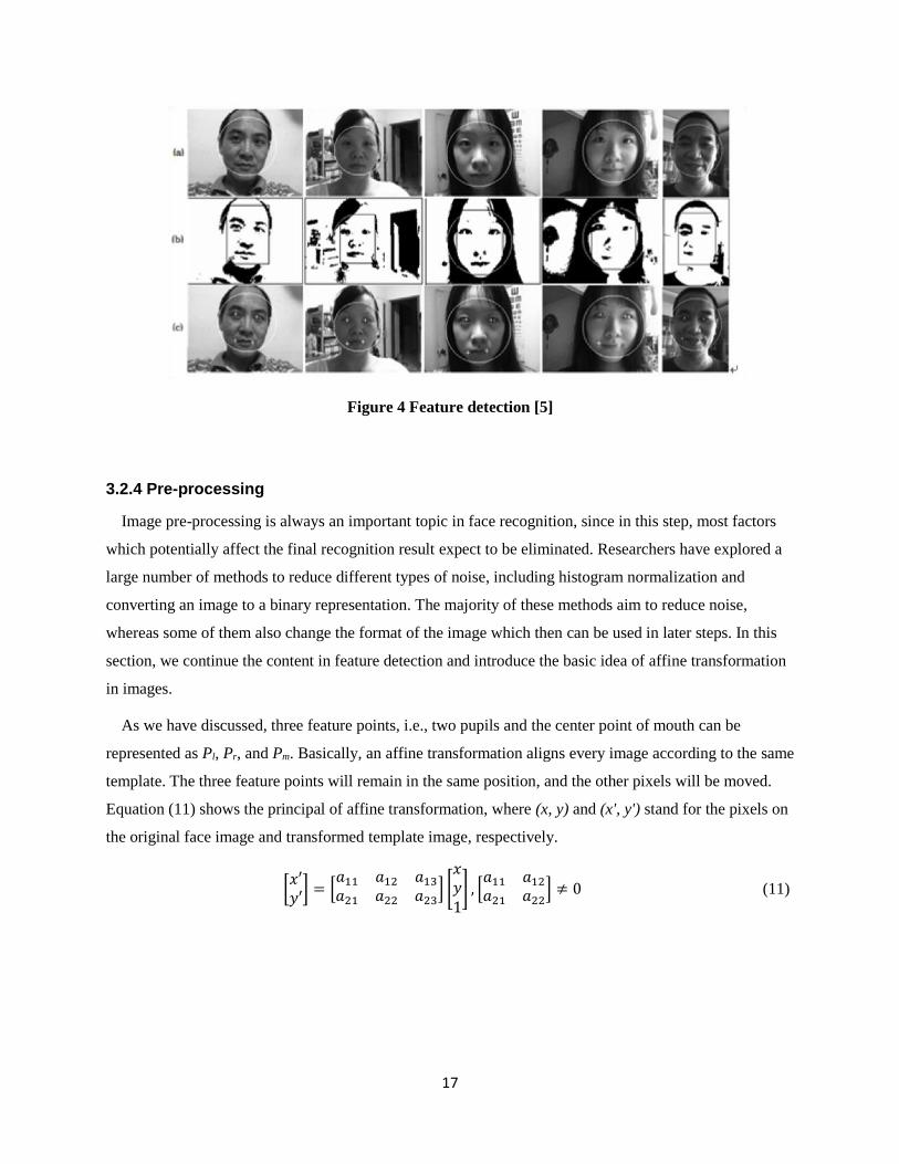
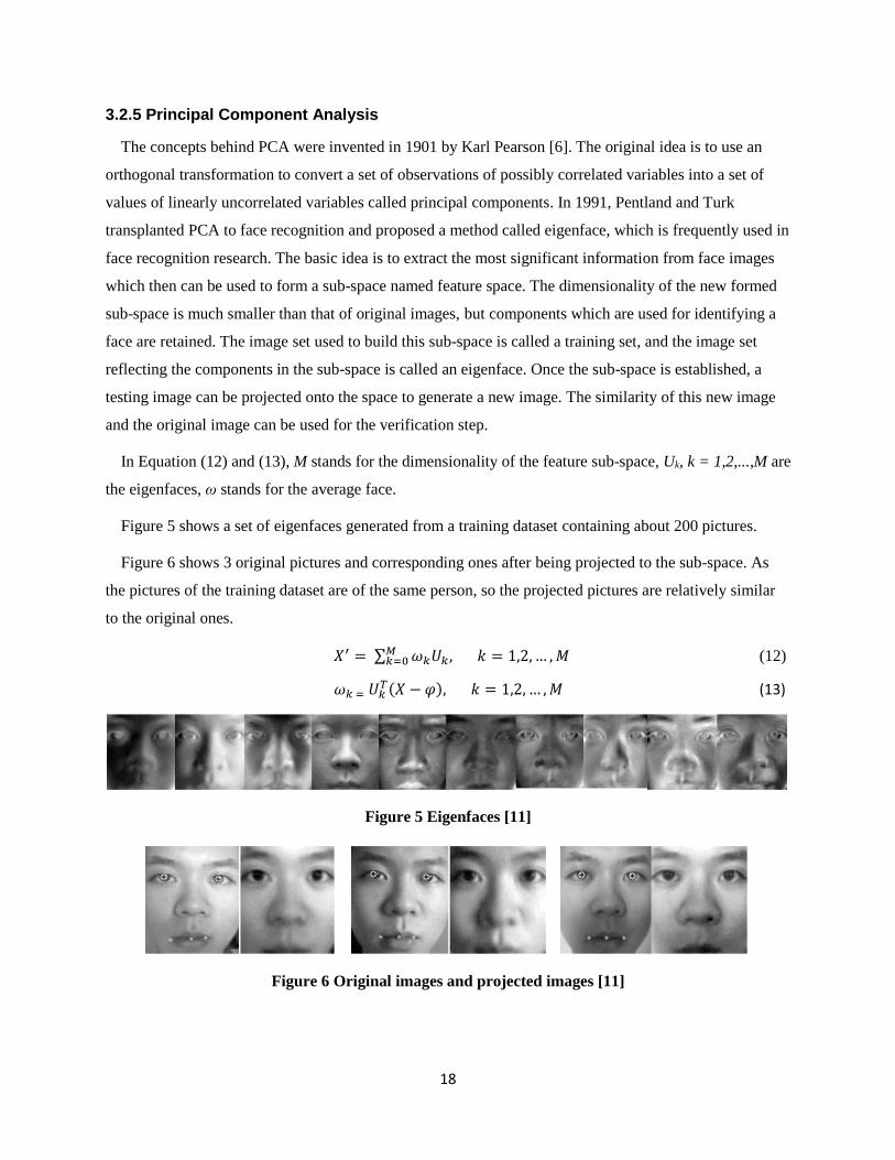
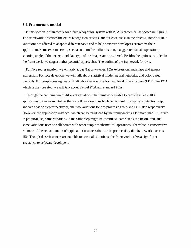
c. Shape & Texture
88
The code for Shape & Texture is not found; however, here we provide two references where possible
implementation thinkings might be obtained [48] [49].
2. Face Detection
a. Statistical Model
For the statistical model, we present codes for LDA method implementation provided by
Zhou Li [40].
#include <stdio.h> #include <stdlib.h> #include <string.h> #include "lda.h" #include "file_access.h" //test code #include <fstream> #include <iostream> #include "document.h" #include "time.h" using namespace std; clock_t start, finish; //test code #include "file_access.h" void init_param(struct corpus *cps,struct est_param* param,int topic_num); // ./lda topic_num sample_num data model_name int main(int argc, char *argv[]) { if ( argc < 5 ) { printf("usage: ./lda topic_num sample_num data model_name\n"); return 0; } int topic_num = atoi(argv[1]); int sample_num = atoi(argv[2]); // how many samples we want, we use these sample's to calculate phi and theta respectively and then use their averge to represent theta and phi char * data = argv[3]; string model_name = argv[4]; int burn_in_num = 1000; //how many iterations are there until we are out of burn-in period // set beta = 0.1 and alpha = 50 / K double beta = 0.1; double alpha = (double)50 / (double)topic_num; int SAMPLE_LAG = 10; struct corpus *cps; struct est_param param; cps = read_corpus(data); init_param(cps,¶m,topic_num); cout << "parameter initialized" << endl; //do gibbs_num times sampling and compute averge theta,phi
89
// burn in period //for (int iter_time=0; iter_time<burn_in_num + sample_num * SAMPLE_LAG; iter_time++) int iter_time = 0; int sample_time = 0; int p_size = topic_num<2?2:topic_num; double *p = (double*)malloc(sizeof(double)*p_size); //multinomial sampling tempoary storage space; double vbeta = cps->num_terms * beta; // v*beta is used in funciton sampling and this value never change so I put it here while (1) { start = clock(); cout << "start sampling all document" << endl; //foreach documents, apply gibbs sampling for (int m=0; m<cps->num_docs; m++) { int word_index = 0; // word_index indicates that a word is the (word_index)th word in the document. double s_talpha = param.nd_sum[m] - 1 + topic_num * alpha; //nd_num[m]+topic_num * alpha will not change per document, so I put it here for (int l=0; l<cps->docs[m].length; l++) { for (int c=0; c<cps->docs[m].words[l].count; c++) { param.z[m][word_index] = sampling(m,word_index,cps->docs[m].words[l].id,topic_num,cps,¶m,alpha,beta,p,s_talpha,vbeta); word_index++; } } } finish = clock(); double dur = (double)(finish - start) / CLOCKS_PER_SEC; cout << "total time : " << dur << endl; if ((iter_time >= burn_in_num) && (iter_time % SAMPLE_LAG == 0)) { calcu_param(¶m, cps,topic_num,alpha,beta); cout << "\t" << sample_time+1 <<"# phi,theta calulation completed" << endl; sample_time++; } cout << iter_time+1 <<"# iteration completed"<<endl; iter_time++; if (sample_time ==sample_num) { break; } } // calculate average of phi and theta cout << "calculating the average of phi and theta" << endl; average_param(¶m, cps,topic_num,alpha,beta,sample_num); cout << "parameter estimation completed, now saving model" << endl; save_model(cps,¶m,model_name,alpha,beta,topic_num,sample_num); /* //test code
90
ofstream out("ap.txt"); for (int i=0; i<cps->num_docs; i++) { out << cps->docs[i].length << " "; for (int j=0; j < cps->docs[i].length; j++ ) { out << cps->docs[i].words[j].id << ":" << cps->docs[i].words[j].count; if (j!=cps->docs[i].length-1) { out << " "; } } out << endl; } out.close(); //test code */ /* //test code for (int d=0; d<cps->num_docs; d++) { int word_index = 0; // word_index indicates that a word is the (word_index)th word in the document. int doc_length = 0; for (int l=0; l<cps->docs[d].length; l++) { for (int t=0; t<cps->docs[d].words[l].count; t++) { cout << param.z[d][word_index] << " "; word_index++; } } } //test code */ return 0; } int sampling(int m, int n, int word_id, int topic_num, struct corpus* cps, struct est_param *param,double alpha, double beta,double* p,double s_talpha,double vbeta) { int topic_id = param->z[m][n]; param->nw[topic_id][word_id]--; param->nd[m][topic_id]--; param->nw_sum[topic_id]--; p[0] = (param->nw[0][word_id] + beta) / (param->nw_sum[0] + vbeta) * (param->nd[m][0] + alpha) / s_talpha; p[1] = p[0]; for (int k = 1; k < topic_num-1; k++) { p[k] += (param->nw[k][word_id] + beta) / (param->nw_sum[k] + vbeta) * (param->nd[m][k] + alpha) / s_talpha; p[k+1] = p[k];
for (int v=0; v<cps->num_terms; v++) { param->phi[k][v] += (param->nw[k][v] + beta) / (param->nw_sum[k] + cps->num_terms * beta); } } } void set_zero(int **a,int rows,int columns) { for (int i=0; i<rows; i++) { for (int j=0; j<columns; j++) { a[i][j] = 0; } } } void set_zero_double(double **a,int rows,int columns) { for (int i=0; i<rows; i++) { for (int j=0; j<columns; j++) { a[i][j] = 0; } } } void init_param(struct corpus *cps, struct est_param* param,int topic_num) { //1. alloc z[m][n], z[m][n] stands for topic assigned to nth word in mth document param->z = (int**)malloc (sizeof(int*) * cps->num_docs); for (int i=0; i<cps->num_docs; i++) { param->z[i] = (int*)malloc (sizeof(int) * cps->docs[i].num_term); } //2. alloc theta[m][k], theta[m][k] stands for the topic mixture proportion for document m param->theta = (double**)malloc (sizeof(double*) * cps->num_docs); for (int j=0; j<cps->num_docs; j++) { param->theta[j] = (double*)malloc (sizeof(double) * topic_num); } set_zero_double(param->theta,cps->num_docs,topic_num); //3. alloc phi[k][v], phi[k][v] stands for the probability of vth word in vocabulary is assigned to topic k param->phi = (double**)malloc (sizeof(double*) * topic_num); for (int z=0; z<topic_num; z++) { param->phi[z] = (double*)malloc (sizeof(double) * cps->num_terms); } set_zero_double(param->phi,topic_num,cps->num_terms);
93
//4. alloc nd[m][k], nd[m][k] stands for the number of kth topic assigned to mth document param->nd = (int**)malloc (sizeof(int*) * cps->num_docs); for (int m=0; m< cps->num_docs; m++) { param->nd[m] = (int*)malloc(sizeof(int) * topic_num); } set_zero(param->nd, cps->num_docs, topic_num); //5. alloc nw[k][t], nw[k][t] stands for the number of kth topic assigned to tth term param->nw = (int**)malloc (sizeof(int*) * topic_num); for (int n=0; n < topic_num; n++) { param->nw[n] = (int*)malloc(sizeof(int) * cps->num_terms); } set_zero(param->nw, topic_num, cps->num_terms); //6. alloc nd_sum[m], nd_sum[m] total number of word in mth document param->nd_sum = (int*)malloc(sizeof(int)*cps->num_docs); memset(param->nd_sum,0,sizeof(int)*cps->num_docs); //7. alloc nw_sum[k], nw_sum[k] total number of terms assigned to kth topic param->nw_sum = (int*)malloc(sizeof(int)*topic_num); memset(param->nw_sum,0,sizeof(int)*topic_num); //8. init nd[m][k],nw[k][t],nd_sum[m],nw_sum[k] srandom(time(0)); // set seed for random function for (int d=0; d<cps->num_docs; d++) { int word_index = 0; // word_index indicates that a word is the (word_index)th word in the document. for (int l=0; l<cps->docs[d].length; l++) { for (int t=0; t<cps->docs[d].words[l].count; t++) { param->z[d][word_index] = (int)(((double)random() / RAND_MAX) * topic_num); // set z randomly param->nw[param->z[d][word_index]][cps->docs[d].words[l].id] ++; param->nd[d][param->z[d][word_index]]++; param->nw_sum[param->z[d][word_index]]++; word_index++; } } param->nd_sum[d] += word_index; } }
b. Neural Network
The code is provided by [41].
int main()
94
{ //Setup the BPNetwork CvANN_MLP bp; // Set up BPNetwork's parameters CvANN_MLP_TrainParams params; params.train_method=CvANN_MLP_TrainParams::BACKPROP; params.bp_dw_scale=0.1; params.bp_moment_scale=0.1; //params.train_method=CvANN_MLP_TrainParams::RPROP; //params.rp_dw0 = 0.1; //params.rp_dw_plus = 1.2; //params.rp_dw_minus = 0.5; //params.rp_dw_min = FLT_EPSILON; //params.rp_dw_max = 50.; // Set up training data float labels[3][5] = {{0,0,0,0,0},{1,1,1,1,1},{0,0,0,0,0}}; Mat labelsMat(3, 5, CV_32FC1, labels); float trainingData[3][5] = { {1,2,3,4,5},{111,112,113,114,115}, {21,22,23,24,25} }; Mat trainingDataMat(3, 5, CV_32FC1, trainingData); Mat layerSizes=(Mat_<int>(1,5) << 5,2,2,2,5); bp.create(layerSizes,CvANN_MLP::SIGMOID_SYM);//CvANN_MLP::SIGMOID_SYM //CvANN_MLP::GAUSSIAN //CvANN_MLP::IDENTITY bp.train(trainingDataMat, labelsMat, Mat(),Mat(), params); // Data for visual representation int width = 512, height = 512; Mat image = Mat::zeros(height, width, CV_8UC3); Vec3b green(0,255,0), blue (255,0,0); // Show the decision regions given by the SVM for (int i = 0; i < image.rows; ++i) for (int j = 0; j < image.cols; ++j) { Mat sampleMat = (Mat_<float>(1,5) << i,j,0,0,0); Mat responseMat; bp.predict(sampleMat,responseMat); float* p=responseMat.ptr<float>(0); float response=0.0f; for(int k=0;k<5;i++){ // cout<<p[k]<<" "; response+=p[k]; } if (response >2) image.at<Vec3b>(j, i) = green; else image.at<Vec3b>(j, i) = blue; } // Show the training data int thickness = -1; int lineType = 8; circle( image, Point(501, 10), 5, Scalar( 0, 0, 0), thickness, lineType); circle( image, Point(255, 10), 5, Scalar(255, 255, 255), thickness, lineType);
95
circle( image, Point(501, 255), 5, Scalar(255, 255, 255), thickness, lineType); circle( image, Point( 10, 501), 5, Scalar(255, 255, 255), thickness, lineType); imwrite("result.png", image); // save the image imshow("BP Simple Example", image); // show it to the user waitKey(0); }
c. Color-based
The code is provided by [43].
function BinImg = GetFaceBin(rgb) Ycbcr = rgb2ycbcr(rgb); fThreshold = 0.22; [M,N,D]=size(Ycbcr); FaceProbImg = zeros(M,N,1); BinImg = uint8(zeros(M,N,1)); Mean = [117.4316 148.5599]'; C = [97.0946 24.4700; 24.4700 141.9966]; cbcr = zeros(2,1); for i=1:M for j=1:N cbcr(1) = Ycbcr(i,j,2); cbcr(2) = Ycbcr(i,j,3); FaceProbImg(i,j)=exp(-0.5*(cbcr-Mean)'*inv(C)*(cbcr-Mean)); if FaceProbImg(i,j)>fThreshold BinImg(i,j) = 1; end end end se=strel('disk',3'); BinImg = imopen(BinImg,se); imdilate(BinImg,se); % subplot(122);imshow(BinImg*255);title(''); CC = bwconncomp(BinImg);
numPixels = cellfun(@numel,CC.PixelIdxList);。
[biggest,idx] = max(numPixels); for i=1:CC.NumObjects if i~=idx BinImg(CC.PixelIdxList{i}) = 0; end end % figure(2);imshow(uint8(BinImg*255)); end
3. Pre-processing
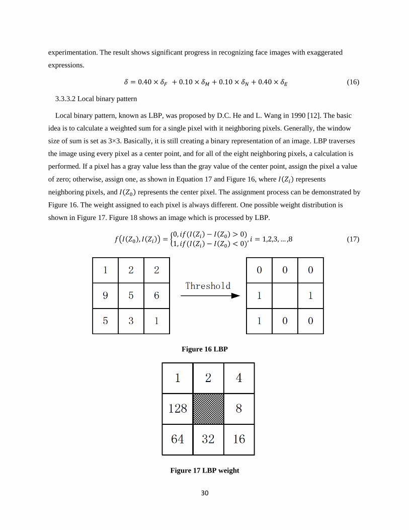
a. Face Seperation
Mat warp_dst = GetAffinedMat(tmpImgCopy2, frame_gray);
96
IplImage *imgLbpSrc = (&(IplImage)warp_dst); IplImage *imgLbpDst = cvCreateImage(cvGetSize(imgLbpSrc), IPL_DEPTH_8U,1);; m_lbpInst.CreatLBP(imgLbpSrc, imgLbpDst); Mat lbp_dst(imgLbpDst); Rect roi(51, 19, 80, 89); Mat matRoi = lbp_dst(roi); m_vmatLbpFace.push_back(matRoi); Rect eyesRoi(46, 22, 84, 38); Mat matEyes = lbp_dst(eyesRoi); m_vmatLbpEyes.push_back(matEyes); Rect mouthRoi(69 ,102, 38, 22); Mat matMouth = lbp_dst(mouthRoi); m_vmatLbpMouth.push_back(matMouth); Rect NoseRoi(71, 57, 39, 37); Mat matNose = lbp_dst(NoseRoi); m_vmatLbpNose.push_back(matNose);
b. LBP
void CLBP::CreatLBP(IplImage *src,IplImage *dst) { int iTemp[8] = {0}; CvScalar s; IplImage *ImgTemp = cvCreateImage(cvGetSize(src), IPL_DEPTH_8U, 1); uchar *data = (uchar*)src->imageData; int iStep = src-> widthStep; for (int i=1;i<src->height-1;i++) for(int j=1;j<src->width-1;j++){ int sum=0; if(data[(i-1)*iStep+j-1]>data[i*iStep+j]) iTemp[0]=1; else iTemp[0]=0; if(data[i*iStep+(j-1)]>data[i*iStep+j]) iTemp[1]=1; else iTemp[1]=0; if(data[(i+1)*iStep+(j-1)]>data[i*iStep+j]) iTemp[2]=1; else iTemp[2]=0; if (data[(i+1)*iStep+j]>data[i*iStep+j]) iTemp[3]=1; else iTemp[3]=0; if (data[(i+1)*iStep+(j+1)]>data[i*iStep+j])


![Human Face Recognition Using PCA with BPNN · Block diagram of complete process of PCA & BPNN face recognition system [12] As shown in this above block diagram I had described about](https://static.documents.pub/doc/80x56/5f6753df354370019f056e91/human-face-recognition-using-pca-with-bpnn-block-diagram-of-complete-process-of.jpg)


