March 2009 Marta Molinas, ELKRAFT Jan Arild Wiik, Tokyo Institute of Technology Master of Science in Energy and Environment Submission date: Supervisor: Co-supervisor: Norwegian University of Science and Technology Department of Electrical Power Engineering A Solution for Low Voltage Ride Through of Induction Generators in Wind Farms using Magnetic Energy Recovery Switch Olav Jakob Fønstelien
Transcript
March 2009Marta Molinas, ELKRAFTJan Arild Wiik, Tokyo Institute of Technology
Master of Science in Energy and EnvironmentSubmission date:Supervisor:Co-supervisor:
Norwegian University of Science and TechnologyDepartment of Electrical Power Engineering
A Solution for Low Voltage RideThrough of Induction Generators inWind Farms using Magnetic EnergyRecovery Switch
Olav Jakob Fønstelien
Problem DescriptionPower electronics converters are used on all types of devices at generation, load andcompensation levels; ranging from low power applications such as light dimmers and motors toMW level power conversion for generation systems. The main features that demand the use ofpower electronics are the requirements of controllability andthe possibility to improve efficiency.
The Magnetic Energy Recovery Switch (MERS) is a new converter topology that has been proposeda decade ago and systematic investigations of the concept have been carried out in Japan. Thisproject will be focused on the implementation of the MERS to enhance the stability of an inductiongenerator.
The project will be realised in Japan at Tokyo Institute of Technology with the cooperation of FujiElectric Device Technology Co., Ltd.
Assignment given: 08. September 2008Supervisor: Marta Molinas, ELKRAFT
A Solution for
Low Voltage Ride Through of
Induction Generators in Wind Farms
using Magnetic Energy Recovery Switch
Master Thesis in Electric Power EngineeringTET4900
Norwegian University of Science and Technology
Olav Jakob Fønstelien, 2009
Abstract
Induction generators constitute 30 percent of today’s installed wind power. They
are very sensitive to grid voltage disturbances and need retrofitting to enhance
their low voltage ride through (LVRT) capability. LVRT of induction generators by
shunt-connected FACTS controllers such as STATCOMs have been proposed in
earlier studies. However, as this report concludes, in this application their VA-
rating requirement is considerably higher than that of series-connected FACTS
controllers.
One such series FACTS controller is the magnetic energy recovery switch
(MERS). It consists of four power electronic switches and a capacitor in a
configuration identical to the single-phase full bridge converter. Its arrangement
in an electric circuit, however, is different, with only two of the converter’s
terminals utilised and connected in series. It has the characteristic of a variable
capacitor and is related to FACTS controllers with series capacitors such as the
GCSC and the TCSC.
Successful operation of MERS for LVRT of induction generators has been
demonstrated by simulations and verified by small-scale experiments.
Index terms – Low voltage ride through (LVRT), magnetic energy recovery switch
At Tokyo Institute of Technology the properties of the magnetic energy recovery
switch have been investigated for some years now. Together, the university and
Fuji Electric Device Technology Co., Ltd. have founded a joint venture,
MERSTech, Inc., which works towards implementing the technology in different
industrial applications.
The work described in this report deals with a new application and has been
carried out in cooperation with Jan Arild Wiik of Tokyo Institute of Technology. It
has been conducted as part of his doctoral thesis, in which he investigates the
MERS in general in addition to the LVRT-application accounted for here. The
thesis is expected to be published in 2009.
I take the opportunity to express my gratefulness to my supervisor Prof. Marta
Molinas of Norwegian University of Science and Technology and to Prof. Ryuichi
Shimada of Tokyo Institute of Technology for letting me visit the Shimada
Laboratory for four months while working on this master thesis. Also, I thank Mr.
Wiik for his friendship and excellent guidance during my stay there.
Olav Jakob Fønstelien
Grimstad, Norway
March 2nd 2009
Table of contents
1 Introduction 1
1.1 Background 2
1.2 Purpose and novelty of work 2
1.3 Contents of report 4
2 Basic concepts of wind generator technology and wind power 5
2.1 Wind power physics 5
2.2 Wind generator technologies 6
3 Grid codes and low voltage ride through (LVRT) of wind farms 9
3.1 Grid codes 9
3.2 LVRT-technologies 10
3.2.1 LVRT of variable speed generators 10
3.2.2 LVRT of fixed speed induction generators 12
4 Simulation study of LVRT of induction generators by idealised 14
shunt and series devices
4.1 Designing the wind farm simulation model 15
4.1.1 Mechanics, capacitor bank and grid 15
4.1.2 Grid fault 18
4.2 Implementing LVRT-devices 20
4.2.1 Phase-locked loop 20
4.2.2 Shunt-connected LVRT-device 24
4.2.3 Series-connected LVRT-device 26
4.3 Simulation model with LVRT-devices 28
4.4 Simulations and results 29
4.4.1 Comparison of performances 30
4.4.2 Comparison of required VA-ratings 33
5 Applying MERS for LVRT of induction generators 38
5.1 MERS 38
5.1.1 Two modes of operation 39
5.1.2 Harmonics and optimum capacitance 42
5.1.3 Comparing MERS to other series-connected 43
FACTS controllers
5.2 Implementing MERS into wind farm model 46
5.3 Simulations and results 51
6 Experimental verification of MERS in the LVRT-application 54
6.1 Laboratory model 54
6.2 Experimental results 59
7 Discussion (with proposals for future works) 64
8 Conclusion 66
References 67
Appendices 69
1 Introduction For some years now it has been an expressed wish of governments around the world to increase the share of renewable energy in the power production. The motivation has mainly been energy security, rising prices of carbon based energy carriers and the prospect of global warming. Concerning the latter, most of the world's developed countries have agreed to reduce their greenhouse gas emissions by signing the Kyoto Protocol to the United Nations Framework Convention on Climate Change [1] and have introduced different schemes for how to reach the goals stated there. The European Union is working towards a 20 percent share of renewables in its energy mix by year 2020 (eight today) [2]. Government funding programs and increased interest from industry and researchers have given rise to a renewable electric energy industry growing by 25 percent a year [3]. The largest contributor to this gain in renewable electric energy is wind power, which has already come to represent a considerable part of the electricity production in some European countries, most notably Denmark, Spain and Germany. Germany alone has an installed effect of about 24 GW, one third of the worldwide total and corresponding to about 20 percent of the country's peak load. Its government wants to double this by 2020, with most of the increase located offshore [4]. In Norway the penetration of wind power is still very low (0.4 GW [5]), but the potential is high. The few wind farms and wind power units (WPUs) already existing are located on the thinly populated western coast. Although the infrastructure is missing, the harsh weather of this region makes it an attractive area since the mechanical power that can potentially be harvested from the wind increases with the cube of the wind speed;
3m winP v∝ d , (1.1)
meaning that a 10 percent rise in wind speed gives about 30 percent rise in power output. Therefore, there are great plans for developing the wind power industry in this region, both on- and offshore. Different concepts have been proposed by Norwegian companies like StatoilHydro [6] and SWAY [7]. According to one study, the total potential may be as high as 14,000 TWh per year [8], with the only restriction being economic feasibility. The Norwegian Ministry of Petroleum and Energy states in a report [8] that it expects between five and eight GW to have been installed offshore by 2020-2025. This would give about 20 TWh yearly, corresponding to approximately 15 percent of today’s national consumption.
1
1.1 Background In addition to that of the uncertainty of weather forecasts, a great concern when integrating wind power into the utility grid is the consequences of grid voltage disturbances. If the grid voltage drops, for instance because one or more of the grid's phases are short-circuited, the electromagnetic torque of the wind generator also drops. But the driving torque, which is the wind, remains unchanged and the resulting imbalance lets the rotor accelerate. Depending on the strength of the wind and the length of the fault, the current in the machine might become high enough to trip the over-current protection system and disconnect from the grid [9]. Regarding this, to ensure power stability, utility grid operators are introducing new rules in their grid codes. These rules state under which circumstances wind farms may disconnect and under which they must continue supplying the grid [4][10]. To enable wind power plants to meet these new demands, different methods for improving their operational stability have been suggested and are referred to as strategies for low voltage ride through (LVRT) of wind farms. A standard procedure, however, has not yet been established, but different solutions for the various generator types available have been suggested. WPUs with synchronous generators may use power electronics to simply lead the energy absorbed during the fault into a dump load or into an energy storage system [11]. As to WPUs with induction generators, the stators are directly connected to the grid and need the grid voltage to be able to draw out energy from the rotor. In the case of doubly fed induction generators, smart use of the rotor's power electronic converters can help uphold the stator voltage during and after the fault, as suggested in [12], whereas the classic squirrel cage generators can be helped by injecting reactive power into the grid and thereby boosting the generator voltage, as described in [13][14][3].
1.2 Purpose and novelty of work Before 2003 there were no demands from utility grids for an LVRT-strategy of wind power installations, but in that year E.ON-Netz of Germany was the first to implement them into their grid code [4][15], and today most grid operators have followed suit. Also before 2003, most WPUs utilised simple squirrel cage induction generators (SCIGs). Because of the direct coupling to the grid, which ties their speed to the grid frequency, they have largely been abandoned for variable speed generators. However, SCIGs still constitute 30 percent of today’s installed wind power [3] and most of the WPUs are fairly new and will be operating for many years still. To allow this they need retrofitting.
2
The most commonly suggested LVRT-strategy for SCIG WPUs is the application of static synchronous compensators (STATCOMs). In this report LVRT by a new power electronic device called magnetic energy recovery switch (MERS) is to be investigated. In contrast to shunt-connected devices like STATCOMs and SVCs, MERS is a series connected FACTS controller. Roughly, its characteristic can be said to be a combination of those of the GCSC and TCSC. In terms of VA-rating, series compensation is more efficient than shunt compensation for increasing a system's energy transmission capability [16]. See figure 1. The work described in this report is motivated by the expectation that the required rating of a series FACTS controller will be considerably lower than that of a shunt device. Since the post-fault generator current will be fairly high, injecting capacitive voltages with a series device like MERS to cancel inductive voltage drops seems more efficient than injecting capacitive currents through shunt devices to cancel inductive currents.
Figure 1: Illustrating the difference between series - and shunt compensation. The phasor diagrams show the difference in magnitude (pu values) of the series-injected voltage and the shunt-injected current when compensating for the voltage drop over a transmission line. Note that to the power plant the grid has the characteristics of a capacitive load.
3
1.3 Contents of report This report is structured as follows: Firstly, an introduction to the basic concepts of wind power and the different technologies existing is given. A discussion of the grid connection rules or grid codes concerning wind power installations is followed by a description of some techniques for enhancing the operational stability of the various generator types. Secondly, a simulation study investigating and comparing the performances of idealised shunt- and series-connected FACTS controllers in this application is carried out. The development of the simulation model used is detailedly described. The model represents on a pu-basis a wind farm subjected to E.ON-Netz’ grid code and contains one 2-MW wind turbine. Before studying the properties of MERS in the wind farm model, its basic characteristics are discussed. Its performance in the LVRT-application is studied and compared to that of the idealised series device. PSIM simulation models are given in the appendices. Thirdly, the basic properties of MERS in the LVRT-application are verified by experiments on a small-scale wind farm model. Proposals for further studies and a discussion of the findings follows after the experiments and the report ends by drawing the conclusions.
4
2 Basic concepts of wind generator technology and wind power A short introduction to the basic physics behind wind power in general and to some of the different wind generators available follows in this chapter.
2.1 Wind power physics The mechanical power drawn from the wind by a turbine is given as
2 3m turbine air wind p2
P R v Cπ ρ= × , (2.1)
where ρair is the air density, Rturbine is the rotor radius and vwind is the wind velocity. The last factor is referred to as the coefficient of performance Cp and describes the efficiency of which the rotor harvests the wind’s energy [17]. Its magnitude depends on the pitch angle of the rotor blades β and the so-called tip-speed ratio λ; the ratio between turbine radius, rotational speed and wind velocity:
( )turbine
wind
Rv
λΩ
= . (2.2)
An example of a profile of Cp versus β and λ is given in figure 2. The curve of a given wind turbine must be determined by experiment, but its theoretical maximum value is limited to 16⁄27 ≈ 59.3 percent, as described in Betz’ law [18].
5
windv windvβ
turbineΩ
turbineR
pC -ProfileBlade Profile
Turbine
Figure 2: Picture illustrating the origin of the different parameters in equation 2.1. The Cp-profile shown is taken from [17] and describes how Cp develops for a given wind power turbine with optimum pitch angle β, but varying tip-speed ratios λ.
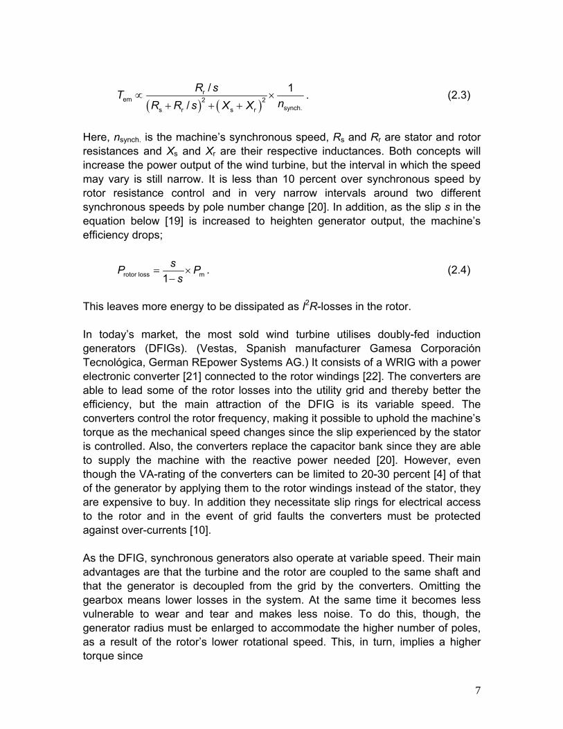
2.2 Wind generator technologies All modern WPUs are able to adjust the turbine blades’ pitch angle to enhance their aerodynamic efficiency, but not necessarily the rotational speed. Objectively therefore, there are two different types of wind generators: Fixed speed generators are operating in a very narrow speed range around their nominal working point. Variable speed generators are able to optimise the speed according to wind velocity and thereby constantly operate at or near the best possible working point. Illustrations of the most common wind generator types are given in figure 3. The classical fixed speed-type utilises SCIGs with the stator connected to the grid and is therefore working at grid frequency. The generator’s rotor is coupled to the turbine through a multi-stage gearbox to increase the rotational speed, which lies in the interval 10-25 rpm. The obvious advantages of SCIGs are low cost and robustness. But the concept is also very vulnerable to grid voltage sags [3] and the generator consumes reactive power which must be provided through a capacitor bank to meet the grid code requirements. In addition the overall aerodynamic efficiency of the rotor is poor since the generator is operating at constant speed. This, however, can to some extent be redressed by wound rotor induction generators (WRIGs) in combination with rheostats. The rheostat is connected to the rotor windings and provides control over the rotor resistance and thereby to some extent the torque-slip characteristics of the machine (Danish manufacturer Vestas Wind Systems A/S). Another possibility is to change the machine’s number of poles and thereby the its synchronous speed (Vestas and Germany’s Siemens AG). Both properties are described by the equation for developed electromagnetic torque [19]:
6
( ) ( )
rem 2 2
synch.s r s r
/ 1/
R sTnR R s X X
∝+ + +
× . (2.3)
Here, nsynch. is the machine’s synchronous speed, Rs and Rr are stator and rotor resistances and Xs and Xr are their respective inductances. Both concepts will increase the power output of the wind turbine, but the interval in which the speed may vary is still narrow. It is less than 10 percent over synchronous speed by rotor resistance control and in very narrow intervals around two different synchronous speeds by pole number change [20]. In addition, as the slip s in the equation below [19] is increased to heighten generator output, the machine’s efficiency drops;
rotor loss m1sP
s= ×P
−. (2.4)
This leaves more energy to be dissipated as I2R-losses in the rotor. In today’s market, the most sold wind turbine utilises doubly-fed induction generators (DFIGs). (Vestas, Spanish manufacturer Gamesa Corporación Tecnológica, German REpower Systems AG.) It consists of a WRIG with a power electronic converter [21] connected to the rotor windings [22]. The converters are able to lead some of the rotor losses into the utility grid and thereby better the efficiency, but the main attraction of the DFIG is its variable speed. The converters control the rotor frequency, making it possible to uphold the machine’s torque as the mechanical speed changes since the slip experienced by the stator is controlled. Also, the converters replace the capacitor bank since they are able to supply the machine with the reactive power needed [20]. However, even though the VA-rating of the converters can be limited to 20-30 percent [4] of that of the generator by applying them to the rotor windings instead of the stator, they are expensive to buy. In addition they necessitate slip rings for electrical access to the rotor and in the event of grid faults the converters must be protected against over-currents [10]. As the DFIG, synchronous generators also operate at variable speed. Their main advantages are that the turbine and the rotor are coupled to the same shaft and that the generator is decoupled from the grid by the converters. Omitting the gearbox means lower losses in the system. At the same time it becomes less vulnerable to wear and tear and makes less noise. To do this, though, the generator radius must be enlarged to accommodate the higher number of poles, as a result of the rotor’s lower rotational speed. This, in turn, implies a higher torque since
7
emem
m
PTω
= , (2.5)
and therefore a need for a larger stator surface. In the case of electrically excited synchronous generators (EESGs), the large surface is needed to avoid magnetic saturation of the iron in the machine, whereas the permanent magnet synchronous generators (PMSGs) need it simply to accommodate the PMs. The speed control of a PMSG is achieved through the application of a power electronic converter between the grid and the stator, and through the application of converters between the grid and both stator and rotor for an EESG. Which of the generator technologies to select depends largely on the price of copper and permanent magnets and the cost of the extra power electronics and control devices needed for the EESG. However, permanent magnet machines have greater flexibility with respect to design, such as radial and axial flux topologies [23]. (EESG-type wind turbines are manufactured by ENERCON GmbH of Germany and PMSG-types by Mitsubishi Power Systems of Japan.)
Figure 3: Illustration showing the main wind generator topologies available on the marked. A. Fixed speed squirrel cage induction generator (SCIG); B. Wound rotor induction generator (WRIG) with rotor windings connected to a rheostat for semi-variable speed; C. Squirrel cage induction generator with two possible pole numbers for semi-variable speed; D. Variable speed doubly-fed induction generator; E. and F. Variable speed electrically excited and permanent magnet synchronous generators (EESG and PMSG, respectively).
8
3 Grid codes and low voltage ride through (LVRT) of wind farms Earlier, wind power installations were disconnected immediately when grid disturbances occurred. This was either to protect power electronic devices from over-currents or in accordance with old operation requirements or grid codes [9]. But, in order to accommodate the ever increasing amount of wind power into the utility grids of Europe, North America and Eastern Asia [24] and in some countries even replace a part of the conventional coal and nuclear power plants [4], stricter demands to the reliability and operation of WPUs have become necessary. Ideally they should be required to behave like other electric power generators. However, given their distinctive character with respect to uncertainty of production forecasts and highly fluctuating output, utility grid operators give them their own grid codes.
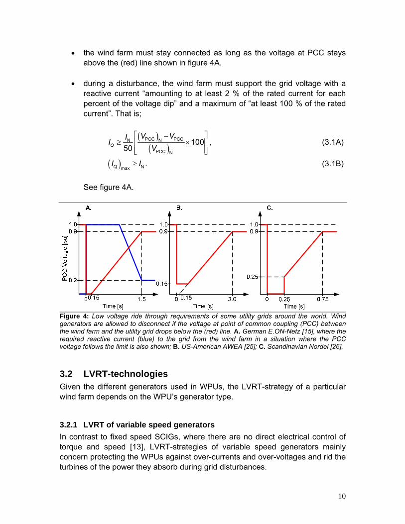
3.1 Grid codes Generally, wind power grid codes describe how a WPU should react to fluctuations in grid frequency, how fast its power output may change and in which power factor interval it must operate. Also, grid codes state how a wind power installation is allowed to behave under the occurrence of grid voltage variations. These may be results of grid faults or sudden losses of large power sources or loads connected to the grid [4][10][15]. The ability of a WPU or a wind farm to withstand voltage variations caused by such grid disturbances is referred to as LVRT-capability. The requirements of a particular grid code depend on the grid’s physical structure and its sources and loads. Some examples are given in figure 4. The main objective of an LVRT-strategy is to make the WPU able to proceed its supply of power to the utility grid in accordance with the grid codes as soon as the grid voltage recovers after a disturbance. In addition it should protect the WPU against over-currents and over-voltages resulting from short circuits as well as supporting the grid voltage with reactive power [4]. For instance, the main requirements of E.ON-Netz’ grid code concerning wind power installations are that
• at PCC the steady state power factor (cos φ) must be greater than 0.95 (inductive)
9
• the wind farm must stay connected as long as the voltage at PCC stays above the (red) line shown in figure 4A.
• during a disturbance, the wind farm must support the grid voltage with a
reactive current “amounting to at least 2 % of the rated current for each percent of the voltage dip” and a maximum of “at least 100 % of the rated current”. That is;
( )
( )PCC PCCN N
PCC N
10050Q
V VIIV
⎡ ⎤−≥ ⎢
⎢ ⎥⎣ ⎦× ⎥
I
, (3.1A)
( ) . (3.1B) ≥ NmaxQI
See figure 4A.
Figure 4: Low voltage ride through requirements of some utility grids around the world. Wind generators are allowed to disconnect if the voltage at point of common coupling (PCC) between the wind farm and the utility grid drops below the (red) line. A. German E.ON-Netz [15], where the required reactive current (blue) to the grid from the wind farm in a situation where the PCC voltage follows the limit is also shown; B. US-American AWEA [25]; C. Scandinavian Nordel [26].
3.2 LVRT-technologies Given the different generators used in WPUs, the LVRT-strategy of a particular wind farm depends on the WPU’s generator type.
3.2.1 LVRT of variable speed generators In contrast to fixed speed SCIGs, where there are no direct electrical control of torque and speed [13], LVRT-strategies of variable speed generators mainly concern protecting the WPUs against over-currents and over-voltages and rid the turbines of the power they absorb during grid disturbances.
10
Synchronous generators (EESGs and PMSGs) are easiest to give LVRT. [11] discusses two different strategies; the first is to apply a dump load controlled by a DC chopper [21] at the stator converter’s DC-link. This way the energy drawn from the rotor during the grid voltage drop is burnt in the resistor while the stator voltage is controlled. A solution with an energy storage system (ESS) is also discussed. Applying an ESS instead of a dump load at the DC-link does not change the behaviour of the WPU during the grid fault, but the device has the advantage of being able to smooth the power output during normal operation. For WPUs with DFIGs several approaches are possible. [12] describes an LVRT-strategy that through smart control doesn’t need any devises or components other than the DFIG’s converters. At the grid-side, the converter can be used to supply reactive power to the system during and after a fault. At the same time it is controlling the DC-link voltage and keeping the stator voltage constant while the rotor-side converter controls the stator’s active and reactive power production and consumption. [4] discusses a solution utilising a crow bar. When a short circuit happens in the grid, current spikes of 5-8 times nominal magnitude are running through the stator. These are reflected on the rotor and may damage the power electronic converters. To protect them, a crow bar is connected between the rotor windings and the rotor-side converter to lead the currents away, as illustrated in figure 5A. However, the current spikes still cause stress in the mechanics connecting the rotor to the turbine since the electromagnetic torque of the machine is very much depending on the stator current, see figure 5B. To curb this, therefore, a triac is disconnecting the stator from the grid when the fault happens. The thyristors open immediately after the fault, but before the current gets too high. The grid-side converter is supplying reactive power while the rotor-side converter synchronises the stator again before it is reconnected. In [10] and [11] a method corresponding to the ESS-approach for synchronous generators discussed above is presented.
11
Figure 5: A. LVRT of a DFIG with crow bar as suggested in [4]; B. Torque on rotor as a result of short circuit current in the stator windings of a DFIG without triac disconnecting the stator. (5B is taken from [4].)
3.2.2 LVRT of fixed speed induction generators The most unstable kind of wind generator is the fixed speed SCIG. The only ways to control it are either to adjust the turbine blades’ pitch angle and thereby their aerodynamic efficiency (Cp) or by varying the voltage applied to the stator. During a grid fault the former is not possible to implement fast enough due to the moment of inertia of the blades, and clearly the latter is not feasible since the stator voltage is the very thing that is out of control. The depth of the voltage drop experienced by SCIGs resulting from a grid fault depends on the location of the fault and on the amount of power produced by synchronous generators in the area. Synchronous generators react to voltage drops by producing reactive power. SCIGs need this to cover their own increased consumption and to cover the lost production of the capacitor banks as well as reactive losses in transformers and power lines [9]. Induction machines cannot work without reactive power simply because they have an inductive characteristic (see [19]). The impedance of an SCIG can be approximated as follows:
( )rSCIG s s r m
ˆ RZ R j X X js
⎛≈ + + +⎜⎝ ⎠
X⎞⎟ . (3.2)
During and after a voltage drop the slip s increases since the rotor is accelerating. The result is a generator impedance that decreases, but that also gets a more inductive character. This means that a higher current is allowed through it and as a consequence it consumes more reactive power. Acceleration of the rotor
12
results from that, for a given slip, the torque developed by the stator is proportional to the applied voltage squared [19]; . (3.3) 2
em sT V∝
However, the acceleration can easily be understood intuitively when considering that the system’s power input stays more or less constant while its power output, which is depending on both current and voltage, is decreased. The energy not absorbed by the grid is accumulated as rotational kinetic energy in the turbine. The main objective of LVRT-strategies for SCIGs is to bring the generator back to its pre-fault operation point after the grid voltage has been restored. To achieve this the turbine must be decelerated, meaning that the stator voltage must be boosted, which again necessitates reactive power. An LVRT-strategy of a 2 MW SCIG WPU based on the reactive power production of a nearby WPU with synchronous generator of equal size is suggested in [3]. Another strategy is to supply reactive power by the application of STATCOMs. In [13] a comparison of the LVRT-performance of a STATCOM and a static var compensator (SVC) is carried out. The STATCOM, basically a shunt-connected reactive current source, is able to provide full output current at voltages down to 0.2 pu, while the SVC, essentially a variable shunt-connected capacitor, has an output maximum linearly increasing with applied AC voltage [16]. In the study it was concluded that the STATCOM had a lover VA-rating than the SVC and therefore that its performance is superior. In [14], where a 10-MVA STATCOM is applied to an existing wind farm consisting of 83 WPUs, the concept is discussed further.
13
4 Simulation study of LVRT of induction generators by idealised shunt and series devices The wind farm discussed in this case study consists of a number of 2 MW SCIG-WPUs in a system layout based on [27]: Each WPU is connected to the farm’s internal grid through a transformer and between them there is placed a capacitor bank for power factor correction. The wind farm is connected to the utility grid that it is supplying through another transformer and it is subjected to E.ON-Netz’ grid codes (figure 4A). An illustration of the wind farm is shown in figure 6 and the parameters are listed in table 1 below. Before discussing MERS in LVRT-applications, a general comparison of shunt- and series-connected LVRT-devices for SCIGs is given in the following chapter. The performance of the two will be judged based on needed VA-rating. But their ability to, after a grid fault, re-establish pre-fault conditions in the system left of PCC in figure 6 below, and to supply both the wind farm and the grid with reactive power during and after the fault is also important and will be discussed. The shunt device will be modelled as a controllable ideal capacitive current source while the series device will be modelled as a controllable ideal capacitive voltage source. To make an as objective as possible comparison, no disturbing control strategies will be applied: The only criterion will be for the two devices to help decelerate the turbine in a given time by injecting a capacitive current or voltage vector of constant magnitude.
AmpI
( )90Shunt Ampˆ vjI I e θ +
=
AmpV
( )90Series Ampˆ ijV V e θ −
=
+ −
inf.V
Figure 6: Illustration of wind farm with transformers and grid and of ideal current and voltage source LVRT-devices. Topology based on [27] and parameters listed in table 1.
14
Squirrel cage induction generator Capacitor bank xCB 2.8 pu (4.8 μF/phase )Nominal voltage VN 0.690 kV WPU trasformer Nominal current IN 1.90 kA V1/V2 0.690/22 [kV] Nominal power PN 2.0 MW Resistance r T WPU 0.008 pu Nominal apparent power SN 2.271 MVA Inductance x T WPU 0.07 pu Nominal slip sN 0.87 % Wind farm trasformer Time constant Htotal 6.3 s V1/V2 22/132 [kV] Stator resistance rs 0.00954 pu Resistance r T WF 0.004 pu Stator inductance xs 0.157 pu Inductance x T WF 0.12 pu Rotor resistance rr 0.0858 pu Grid Rotor inductance xr 0.103 pu Voltage vinf. 1.005 pu Magnetising resistance rm 0.120 pu Resistance rGrid 0.0555 pu Magnetising inductance xm 4.96 pu Inductance xGrid 0.0832 pu Total mom. of inertia Jtotal 285 Nm2 Correction factor k 1.005 Mechanical Torque Tm 6.57 kN m cos φPCC 0.95 (ind.) Base values Base power PBase 2.00 MW Base voltage VBase 0.690 kV Base current IBase 1.90 kA Base impedance ZBase 210 mΩ Table 1: Wind farm data.
4.1 Designing the wind farm simulation model To make the model as simple as possible, a model containing only one generator with the relatively sized grid and transformer parameters represents the whole wind farm. To do this, the model must be designed on a pu-basis. The model is designed in the computer simulation program PSIM by Powersim Inc. [28]. This program has a built-in C [29] compiler and offers tailor made solutions for studying problems relating to electric power engineering. The development of the simulation model will be done in two steps. Firstly, the values of the different parameters needed in the model will be established before a grid fault is implemented. Secondly, a shunt device and a series device for LVRT of the WPU will be designed and implemented into the model, after which their performance will be investigated and compared.
4.1.1 Mechanics, capacitor bank and grid In the simulation model, the designer is free to choose the generator pole number p simply by adjusting the moment of inertia Jtotal of the WPU’s rotating parts according to the equation [30]
15
( ) ( )
total N total Ntotal 2
m Ns
N
2 2
21 2
H S H SJs f
2
pω
π
= =⎛ ⎞
+ ×⎜ ⎟⎝ ⎠
, (4.1)
where Htotal is the system’s mechanical time constant, ωm is the mechanical speed, fs is the applied electrical frequency, SN is the machine’s apparent power and s is the slip. N denotes nominal values. By choosing two poles, which gives equal electrical and mechanical rotational speeds, the total moment of inertia is 285 Nm2 and the nominal speed is 3026 rpm. Ignoring losses, the torque needed to drive the generator at this speed producing 2.0 MW is estimated to be 6.44 kN m. By trying and failing, the value corresponding to the nominal power and slip is found to be 6.57 kN m, which implies that there is a mechanical and electrical loss in the generator totalling 2.1 percent. E.ON-Netz’ grid code demands an inductive power factor at PCC of at least 95 percent. To achieve this in the model, the capacitor bank must be sized properly. The reactive power balance for the system illustrated in figure 7A can be written as follows: . (4.2) PCC T WF T WPU CB N0 q q q q= − + + − + q Here, to meet the grid code requirement, ( )PCC PCC PCCtan 1.00 tan arccos0.95 0.33 puq p ϕ= ≈ × = , (4.3) since, if power losses are neglected, . (4.4) PCC N 1.00 pup p≈ =
Further, the nominal reactive power of the machine can be derived as
2 2N N N 0.54 puq s p= − = . (4.5)
Ignoring the effect of the capacitor bank, the grid current is assumed to be the same as the generator current. A rough first estimate of the reactive power consumed by the two transformers is then given as
. (4.6) ( )2
T WF T WPU N T WF T WPU
2 1.00 (0.07 0.12) 0.19 pu
q q i x x+ ≈ +
= × + =
16
This leaves a reactive power of 0.40 pu to be contributed by the capacitor bank, which implies a capacitor bank current equalling
CBCB
N
0.40 puqiv
= = . (4.7)
Deriving from the phasor diagram in figure 7B the equation (4.8) ( ) (22
grid N N N N CBcos sini i i iϕ ϕ= + − )2
and inserting the capacitor bank current found above, a second, more accurate estimate of the reactive power consumed by the two transformers is
. (4.9) ( )2
T WF T WPU grid T WF T WPU
2 0.88 (0.07 0.12) 0.15 pu
q q i x x+ = +
≈ × + = According to the balance equation, the reactive power produced by the capacitor bank must thus be at least 0.36 pu. This means that the impedance of the capacitor bank equals
2N
CBCB
=2.8 puvxq
= , (4.10)
which corresponds to a capacitance of
( )
CB CB BaseCB 22
N N Base
4.8 mF per phase.Q q PCV v Vω ω
= = = (4.11)
17
PCC T WF T WPU CB N0 q q q q q= − + + − +
PCCcos 0.95ϕ =
Nq
CBq
T WPUq T WFq PCCq
N N,p i
Nv
PCC grid,p i
Ncos 0.88ϕ =
Nϕ
NI
CBI
NVgridI
CBi
Figure 7: A. Illustration of the reactive power balance in the wind farm pu-model; B. Phasor diagram with the vectors of interest in pu-values showing how an estimate of the grid current can be calculated. In terms of power transmission through lines, the lower the impedance the better. But to keep short circuit currents within limits, a certain value is needed. An impedance of 0.1 pu with a ratio between its inductive and resistive part of 3⁄2 limits the short circuit current to ten times the generator’s nominal current and corresponds to the x⁄r -ratio found in real utility grids [31]. To get the desired generator voltage and current, the voltage of the infinite bus must be adjusted with a small correction factor k; . (4.12) inf. BaseV k V= ×
Doing this, however, sets a new base voltage for this part of the circuit, and the grid’s impedance must be adjusted accordingly; . (4.13) new old new 2 old
Base Base Base Base V k V Z k Z= × ⇒ = ×
4.1.2 Grid fault E.ON-Netz demands the wind farm to stay connected as long as the voltage at PCC stays above the voltage curve shown in figure 4A. To test if this is the case for the model with the parameter values found above applied to it, a grid fault is implemented into the model. By means of a controllable voltage source at the grid side, a short circuit with consequent gradual recovery of the voltage is simulated, as shown in figures 8A and 8D. As the short circuit occurs the system is operating in steady state under rated conditions. As illustrated in figure 8B the generator begins to accelerate as soon as the voltage drops. This is because the driving torque is set constant while the electromagnetic torque created by the stator drops as the voltage drops. The
18
assumption of constant driving torque is also made in [13] and is based upon the expectation that the wind driving a real turbine will stay more or less constant during such a short time. Also, the aerodynamic efficiency of the turbine does not change considerably within such a narrow speed interval. In the next phase, when the fault in the grid has been cleared and the voltage has been restored, it can be seen in figure 8B that the acceleration is for a short moment brought to a halt. The PCC voltage, seen in figure 8C, is at 90 percent without having crossed the limit stated in the grid code. This means that the voltage has stayed within the area in which the WPU must stay connected and proceed normal operation. However, immediately afterwards the turbine accelerates further and control over the generator is lost. At this point the generator must be disconnected for not to be a burden to the rest of the power system by drawing too much reactive power (figure 8F).
0
1
2
3
0 1 2 30
0.2
0.4
0.6
0.8
1
0
20
40
60
80
100
0 1 2 30
100
200
0
0.2
0.4
0.6
0.8
1
0 1 2 3
0
0.5
1
-0.5
Grid Impedance
inf. ( )v
x t k=
×
PCC
m
constantT =
WPU Trafo
Wind Farm Trafo
( )x t
Infinite Bus
Cap.Bank
Two-PoleSCIG
( )x t
GridCode
PCC v
SCIGp
Slip
PCCqgridi
PCCq gridi
SCIGp
PCCv
Time [s]
Wind Farm Simulation Model(without LVRT-device)
[%]
[%][%]
[pu] [pu]
[1]
A.
B. C. D.
E. F. G.
0.15
0.44
1.35
SCIGv
SCIGv
Figure 8: A. Schematic presentation of the developed simulation model (pu-values). Data given in table 1 above; B. Curve showing the generator accelerating as the grid voltage dips; C. Voltage at PCC in percent together with the E.ON-Netz grid code. Observe that the voltage curve
19
stays within the allowed area until after the grid voltage has been restored; D. Profile of x(t) fed to the variable voltage source; E. Stator voltage and power flow out of the generator. The area between the dotted line and the power curve is approximately equal to the kinetic energy accumulated in the turbine during the disturbance; F. Reactive power flow into the wind farm from the grid; G. Grid current in percent. The current shoots up as the grid is short-circuited and it settles at a level higher than before due to the lower (slip-dependent) generator impedance [19].
4.2 Implementing LVRT-devices From the curves of figure 8, it is evident that the wind farm, as it is modelled, does not fulfil the stability requirements stated in the grid code. An LVRT-device is therefore needed. As mentioned above, the shunt device, for instance a STATCOM, is to be modelled as an ideal variable current source and the series device, which can be thought of as a MERS, is to be modelled as a voltage source. To control the devices such that they are always perfectly capacitive, the phase angle of (respectively) the line voltage and line current must be known. This is done by basing the control of the devices on a phase-locked loop.
4.2.1 Phase-locked loop The phase-locked loop (PLL) [32] is based on the space vector abc/dq-transformation [33] and is used to track the phase angle of either the current or the voltage at a given point in an electrical circuit. Assume that the three-phase system shown in figure 9A is balanced and that the current and voltage amplitudes both are 1. Let the space vector sx be the vectorial sum of either the line currents or line voltages in the system;
( )( )
a s
s b s
c s
sinsin 2 3sin 2 3
xx x
x
θθ πθ π
⎡ ⎤⎡ ⎤⎢⎢ ⎥= = +⎢⎢ ⎥⎢ ⎥⎢ ⎥ −⎣ ⎦ ⎣ ⎦
⎥⎥ . (4.14)
The length of sx is 3⁄2 and it is rotating counter-clockwise with an angular speed
s 2d fdtθ
ω π= = , (4.15)
where sθ is referred to the perpendicular (-β)-axis and f is the electrical frequency of the three-phase system. Described as a three-dimensional vector, the three-phase current or voltage is overrepresented since of course only two dimensions are needed to describe a vector in a two-dimensional plane. Referred to the reference frame αβ therefore, the current or voltage can also be described by the
20
space vector αβx by transforming the system from the abc to the αβ reference frame:
ααβ abc/αβ s
β
1 1 2 1 223 0 3 2 3 2
xsx x
x− −
x⎡ ⎤⎡ ⎤
= = = ⎢ ⎥⎢ ⎥−⎣ ⎦ ⎣ ⎦
T . (4.16)
abc/αβT is the transformation matrix, appearing when solving the trigonometric
equations that can be derived from figure 9B. contains a factor abc/αβT 2⁄3 converting the space vector length to 1, which is the amplitude of the system’s current or voltage.
a-axis
b-axis
c-ax
is
α-axis
β-axis
sθ
sx
ax
cx
bxbx
cx
α32
x
β32
x
23π
abv
bcvcav
ai
bi
ci
Phase a
Phase b
Phase c
Balanced Three-Phase System
αβx
abc/αβ Transformation Diagram
( )( )
a s
s b s
c s
sinsin 2 3sin 2 3
xx x
x
θθ πθ π
⎡ ⎤⎡ ⎤⎢ ⎥⎢ ⎥= = +⎢ ⎥⎢ ⎥⎢ ⎥⎢ ⎥ −⎣ ⎦ ⎣ ⎦
A. B.
ω
ααβ s
β
1 1 2 1 223 0 3 2 3 2
xx x
x− −⎡ ⎤⎡ ⎤
= = ⎢ ⎥⎢ ⎥−⎣ ⎦ ⎣ ⎦
s αβ3 ; 12
x x= =
Figure 9: Illustration of the abc/αβ transform of a space vector (B.) describing either the line-to-line voltages or the line currents of a balanced three-phase system (A.). The next step is to transform the vector from the stationary αβ reference frame into the rotating dq reference frame of figure 10C. Firstly, let dαθ be the angle between the axes d and α. Then, by solving the trigonometric equations that can be found by analysing the vector diagram, the transformation matrix appears as follows:
dα dααβ/dq
dα dα
cos sinsin cosθ θθ θ
⎡ ⎤= ⎢−⎣ ⎦
T ⎥ . (4.17)
21
The resulting abc/dq transform can then be written as follows:
T
dq d q abc/dq sx x x x⎡ ⎤= =⎣ ⎦ T , (4.18)
where the transformation matrix is given as
abc/dq αβ/dq abc/αβ
dα dα dα dα dα
dα dα dα dα dα
2cos 3 sin cos 3 sin cos1 .3 2sin sin 3 cos sin 3 cos
θ θ θ θ
θ θ θ θ θ
=
⎡ ⎤− − −= ⎢ ⎥
− − +⎢ ⎥⎣ ⎦
T T T
θ (4.19)
The idea now is to let the dq reference frame rotate with the same speed as sx . If it is, dx can be found as (d s αsinx )dθ θ= − , (4.20) and if the difference between the angles is small, dx can be approximated as (d s dαx )θ θ≈ − . (4.21) This implies that by designing a control loop that locks the dq reference frame to the phase angle such that s dα error dxθ θ θ− = ≈ , (4.22) the angle of the space vector is found as s dα d q αβ when is small and 1x x xθ θ≈ ≈ − = − . (4.23)
The PLL control loop, as illustrated in figure 10A, consists of an abc/dq transformation block where the output is fed to a PI-controller followed by an integrator [34] whose output is the angle dαθ [32]. This is fed back to the abc/dq-block and the looped PI-block and integrator control the error to zero, implying that s dαθ θ≈ . If the system voltages or currents are distorted, filtering may be achieved by the use of a technique suggested in [35] and illustrated in figure 10B. Here, the estimate dαω of the angular frequency is sent through a low-pass filter before it is integrated. The cut-off frequency equals the grid frequency. The new
22
phase angle estimate dαθ is then tied to the original estimate dαθ by calculating the difference between them, multiplying this with a factor (50), and integrating the result.
α-axis
β-ax
is
d-axis
q-ax
is
sθ
dαθ
error dxθ ≈
αx
βx
qβx
dβx
dβx
qαx
dαx
qx
dx
αβx
abc/dq
PI ∫d errorx θ≈
dαθ
dαω
Phase-Locked Loop (PLL)
a
s b
c
xx x
x
⎡ ⎤⎢ ⎥= ⎢ ⎥⎢ ⎥⎣ ⎦
αβ/dq Transformation Diagram
dα dαdq αβ
dα dα
cos sinsin cos
x xθ θθ θ
⎡ ⎤= ⎢ ⎥−⎣ ⎦
dα sθ θ≈
length 1=
d errorsinx θ=
abc/dqT
abc/dq
PI ∫
dαθ
a
s b
c
xx x
x
⎡ ⎤⎢ ⎥= ⎢ ⎥⎢ ⎥⎣ ⎦
abc/dqT
−+
K
∫dαω dα sθ θ≈++
Figure 10: A. and B. Schematic presentation of a PLL with [35] and without [32] low-pass filter to deal with current or voltage distortion; C. Vector diagram illustrating the αβ/dq transformation. Observe that equations 4.20 and 4.22 can be derived directly from the diagram.
23
4.2.2 Shunt-connected LVRT-device The shunt device is to be modelled as a perfectly capacitive controllable current source with constant amplitude. The controller must generate a current vector with constant amplitude and phase angle leading the phase voltage vector with 90 degrees. Firstly, a PLL whose input is the space vector sv describing the line-to-line voltages at PCC is utilised to track the phase angle sθ . 30 degrees must be subtracted due to the phase shift between phase and line-to-line voltages. The phase voltages are not measured and used because they need to be referred to the ground, while the line-to-line voltage does not. Secondly, by applying an amplitude Iamp and transforming the resulting space vector from the rotating dq reference frame to the stationary abc reference frame, a current space vector is generated: si [ ]Ts a b c dq/abc dqi i i i i= = T . (4.24) The dq/abc transformation matrix is given as follows;
The length of the space vector is 3⁄2IAmp. The element relating to each phase abc is a time-domain scalar describing a sine curve leading the phase’s voltage with 90 degrees. See figure 11. How to feed the current amplitude can be determined by analysing the vector diagram. It can be seen that, when errorθ in equation 4.22 is small, the (-q)-axis is approximately aligned with the indicated phase voltage space vector. As already mentioned the current vector is to be injected with a 90 degrees’ lead relative to this, which is approximately the d-axis. Therefore, the current space vector is given as
. (4.26) ddq Amp
q
10
ii I
i⎡ ⎤ ⎡ ⎤
= =⎢ ⎥ ⎢ ⎥⎣ ⎦⎣ ⎦
24
(-β)-a
xis
6πd-
axis
q-axis
dq d Amp( ) ( )i t i t I= =
s( )v tdα( )tθ
s( )tθ
s2 ( )3
v t
a( )i t
ab( )v t
phase( )v t
s2 ( )3
i t
( )phase a( )v t
α-axis
ab( )v t
ca( )v t
Phase a
Phase b
Phase c
PLL
a
s b
c
( )( ) ( )
( )
x tx t x t
x t
⎡ ⎤⎢ ⎥= ⎢ ⎥⎢ ⎥⎣ ⎦
6π
−+ dq/abc
dq/abcTAmp
10
I ⎡ ⎤⎢ ⎥⎣ ⎦
×
Enable/Disable
1 or 0
s( )tθdα( )tθ
( )( )( )
a s
b Amp s
c s
( ) sin ( ) 2( ) sin ( ) 7 6( ) sin ( ) 6
i t ti t I ti t t
θ πθ πθ π
⎡ ⎤+⎡ ⎤⎢ ⎥⎢ ⎥ = +⎢ ⎥⎢ ⎥⎢ ⎥⎢ ⎥ −⎣ ⎦ ⎣ ⎦
Amp1V
×
( )( )
ab s
bc Amp s
ca s
( ) sin ( )( ) sin ( ) 2 3( ) sin ( ) 2 3
v t tv t V tv t t
θθ πθ π
⎡ ⎤⎡ ⎤⎢ ⎥⎢ ⎥ = +⎢ ⎥⎢ ⎥⎢ ⎥⎢ ⎥ −⎣ ⎦ ⎣ ⎦
bc ( )v t
a( )i t b( )i t c ( )i t
s( )v t
a
s b
c
( )( ) ( )
( )
x tx t x t
x t
⎡ ⎤⎢ ⎥= ⎢ ⎥⎢ ⎥⎣ ⎦
s( )i t
c ( )i tb( )i t
a( )i t
q( ) 0i t =
s2 ( )3
i t
dq( )i t
Figure 11: Schematic presentation of a control loop for modelling shunt-connected LVRT-devices (such as STATCOMs) as an ideal perfect capacitive current source. The current is injected as a space vector of length IAmp perpendicular to the phase voltage space vector. The PLL is of the type shown in figure 10B above.
25
4.2.3 Series-connected LVRT-device Modelling the series-connected LVRT-device is done in much the same fashion as the shunt-connected. In stead of current sources, controllable voltage sources are utilised and in stead of orienting the control to the system’s voltage it is oriented to its current. Apart from this, the only difference from the shunt-control in the series-control is that the subtraction of 30 degrees is omitted. The device must inject a voltage into each phase that is lagging the phase’s current with 90 degrees. Again, this is done by measuring the current of each phase to derive the phase angle sθ of the resulting current space vector with a PLL. Based on this angle a voltage space vector
si
dqv with amplitude VAmp is generated. In the shunt-control scheme it was shown that the dq current space vector had to be on the form [1 0]T in order to be perfectly capacitive. As illustrated in figure 12, the dq voltage space vector injected into the system by the series-device must be on the form [-1 0]T. That is;
. (4.27) ddq Amp
q
10
vv V
v⎡ ⎤ −⎡ ⎤
= =⎢ ⎥ ⎢ ⎥⎣ ⎦⎣ ⎦
As in the shunt-control, this space vector is dq/abc transformed to get the abc reference frame space vector sv ; [ ]Ts a b c dq/abc dqv v v v v= = T , (4.28) and each phase’s element is fed to the input of controllable voltage sources.
26
(-β)-a
xis
d-ax
isq-axis
dq d Amp( ) ( )v t v t V= =
dα( )tθ
s( )tθ
s2 ( )3
i t
a( )i ta( )v t
α-axisq( ) 0v t = s
2 ( )3
i t
( )( )
a s
b Amp s
c s
( ) sin ( )( ) sin ( ) 2 3( ) sin ( ) 2 3
i t ti t I ti t t
θθ πθ π
⎡ ⎤⎡ ⎤⎢ ⎥⎢ ⎥ = +⎢ ⎥⎢ ⎥⎢ ⎥⎢ ⎥ −⎣ ⎦ ⎣ ⎦
( )( )( )
a s
b Amp s
c s
( ) sin ( ) 2( ) sin ( ) 6( ) sin ( ) 7 6
v t tv t V tv t t
θ πθ πθ π
⎡ ⎤−⎡ ⎤⎢ ⎥⎢ ⎥ = +⎢ ⎥⎢ ⎥⎢ ⎥⎢ ⎥ −⎣ ⎦ ⎣ ⎦
a
b s
c
( )( ) ( )( )
x tx t x tx t
⎡ ⎤⎢ ⎥ =⎢ ⎥⎢ ⎥⎣ ⎦
a
s b
c
( )( ) ( )
( )
x tx t x t
x t
⎡ ⎤⎢ ⎥= ⎢ ⎥⎢ ⎥⎣ ⎦
Amp1 I
×
Amp
10
V−⎡ ⎤⎢ ⎥⎣ ⎦
× Enable/Disable1 or 0
PLL and
dq/abc-Matrix
Phase a
Phase b
Phase c
a( )i t
b( )i t
c ( )i t
Wind Farm PCC Grid
+ −
+ −
+ −
a( )v tb( )v t
c ( )v t
a( )v t
b( )v t
c ( )v t
s( )v t s( )i t
Series-Connected LVRT-Device
s2 ( )3
v ts
2 ( )3
v t
dq( )v t
Figure 12: Illustration of control concept of an ideal series-connected LVRT-device (such as the MERS). The control circuit tracks the phase angle of the system’s current space vector and injects a capacitive voltage space vector in series. The strategy is basically the same as for the shunt-device, except for voltages being replaced by currents and vice versa, and there being no need to subtract 30 degrees from the input space vector angle. See figure 11. The PLL is of the type shown in figure 10A above.
27
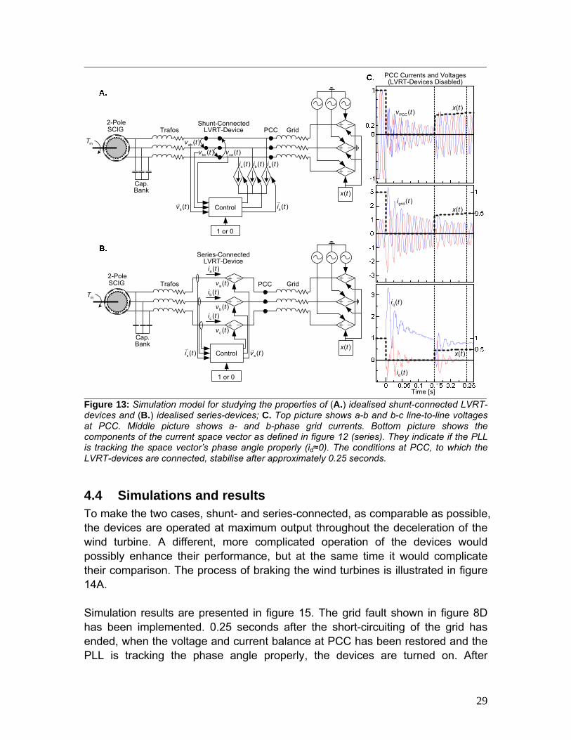
4.3 Simulation model with LVRT-devices Having implemented the idealised LVRT-devices, simulation models for studying the properties of shunt-connected devices such as STATCOMs and series-connected devices such as the MERS in the LVRT-application have been developed. After the grid fault has occurred, as soon as the voltage at PCC reached 20 percent (lower limit of operation for a STATCOM [16]) and the voltage and current are balanced, the devices are turned on. As illustrated in figures 11 and 12, this is done by feeding a “1” instead of a “0” to the multiplication node shown in the control circuits. Figure 13C shows that the voltage immediately jumps over 20 percent as the grid voltage begins to recover. However, as with the current, it needs some time to balance. It can be seen that after approximately 0.25 seconds the voltages and currents are balanced and that the PLL has stabilised and is tracking the current phase angle. At this instance the “1” is fed in both models. While simulating, it is found that the PLL in the control of the shunt device needs some extra filtering. It gets unstable during operation, which is most likely due to the relatively high current it is supplying. The PLL illustrated in figure 10B above is used and keeps the operation stable. For controlling the series device, the somewhat simpler PLL of figure 10A is sufficient. The PSIM simulation models are given in the appendices.
28
+ −
+ −
+ −
+PCC
−
+ −
+ −
+ −
+ −
+ −
PCC
ab( )v t
bc ( )v t ca ( )v t
Control
Control
1 or 0
1 or 0
2-PoleSCIG
2-PoleSCIG
Grid
Grid
Trafos
Trafos
Cap.Bank
LVRT-DeviceSeries-Connected
LVRT-DeviceShunt-Connected
s( )v t
s ( )v t
s ( )i t
s ( )i t
a( )v t
b ( )v t
c ( )v t
c ( )i t
b( )i t
a ( )i t
a ( )i tb( )i tc ( )i t
grid( )i t
PCC( )v t
( )x t
( )x t
Time [s]
Cap.Bank
( )x t
( )x t
mT
mT
PCC Currents and Voltages(LVRT-Devices Disabled)
( )x t
q( )i t
d( )i t
Figure 13: Simulation model for studying the properties of (A.) idealised shunt-connected LVRT-devices and (B.) idealised series-devices; C. Top picture shows a-b and b-c line-to-line voltages at PCC. Middle picture shows a- and b-phase grid currents. Bottom picture shows the components of the current space vector as defined in figure 12 (series). They indicate if the PLL is tracking the space vector’s phase angle properly (id≈0). The conditions at PCC, to which the LVRT-devices are connected, stabilise after approximately 0.25 seconds.
4.4 Simulations and results To make the two cases, shunt- and series-connected, as comparable as possible, the devices are operated at maximum output throughout the deceleration of the wind turbine. A different, more complicated operation of the devices would possibly enhance their performance, but at the same time it would complicate their comparison. The process of braking the wind turbines is illustrated in figure 14A. Simulation results are presented in figure 15. The grid fault shown in figure 8D has been implemented. 0.25 seconds after the short-circuiting of the grid has ended, when the voltage and current balance at PCC has been restored and the PLL is tracking the phase angle properly, the devices are turned on. After
29
another 1.10 seconds the grid voltage has been restored. Decelerating the wind turbine in 1.00 second after this is used as common reference. That is; 2.35 seconds after the short circuit occurred and 1.00 second after it has been fully cleared, the generator must operate at its pre-fault slip. By trying and failing, it is found that this is achieved either by injecting a shunt current of 1.37 pu or by injecting a series voltage of 0.163 pu. By logging the active and reactive power of the modelled devices, it is also found that they are both operating at a power factor of 1.2 percent: , (4.29A) ( )Shuntcos cos 90.7 1.2 %ϕ = = −
with a net consume of active and a net production of reactive power, while ( )Seriescos cos 89.3 1.2 %ϕ = = , (4.29B)
with a net production of both active and reactive power. The power factors stay constant throughout the deceleration period and are possibly indicating that the phase angle estimate dαθ leads the real phase angle of the current or voltage with some 0.7 degrees. If this was the case, the space vector diagrams of figures 11 and 12 would agree with this. However, the power factors show that the devices are working properly and that they have close to perfectly capacitive characteristics.
4.4.1 Comparison of performances Left of PCC, at the wind farm side, the conditions are more or less independent of which of the two LVRT-devices that are being used, see figures 15A through 15D. The currents and voltages as well as the deceleration of the generator are proceeding almost identically. It can be seen that generator pre-fault conditions are not re-established since the SCIG is not operating in steady state as it is decelerated to its nominal rotational speed. Also, the machine’s torque-slip characteristics are changed due to the higher generator voltages. When the system re-enters steady state, it will be at a lower slip than before the fault since the LVRT-devices are still operating and are cancelling the inductive voltage drops of the grid and transformers. See figure 14B. At the grid side of PCC things are drastically different in the two cases, as seen in figures 15E through 15I. Decelerating the SCIG requires large amounts of reactive power. The shunt-connected device makes the needed reactive power available by supplying it itself at PCC. The series-connected device cancels the
30
inductive losses in the grid to increase its transmission capability – transmission capability of both active and reactive power. The result, which could be anticipated, is that the wind farm taps the reactive power that it needs directly from the grid. The influence of this on the stability of the grid is very much depending on its structure, but, as stated in E.ON-Netz’ grid code, this is not allowed (see chapter 3.1). How this problem can be dealt with is uncertain. As for the shunt device, it too cancels the inductive losses in the grid and even supplies it with additional reactive power. The amount, though, is not large enough to meet the demands of the grid operator, according to equation 3.1. This means that the current must be boosted. See figure 15G.
( )x t
+ −
Stator 1 puV >
Stator 1 puV =
Stator 1 puV <
SeriesV
ShuntI
GridI
GridVInf.V
( )x t
( )x t
WFI
WFI
WFV
WFV
WFI
GridI
ShuntI
WFV
WFV
WFI
Inf.V
GridV
SeriesV
WFθ
WFθ
Figure 14: A. Steady state torque-slip characteristics of an SCIG at different voltage levels. Even though the system is not in steady state during a voltage disturbance, the picture illustrates the acceleration at low voltages, deceleration at higher voltages and subsequent steady state operation at a lower slip; B. Phasor diagram showing how the current and voltage vectors are injected (pu-values). Resistive losses are ignored; C. System illustration for the phasor diagram.
31
Figure 15: Curves showing the development of the parameters in the system prior to, during and after the grid fault. A. Generator slip. Decelerating the turbine in 2.35 seconds is set as common reference when comparing the LVRT-strategies; B. The mechanical power input is close to constant while the generator’s output drops immediately after the fault. Observe that the overall area between the series/shunt-curve and the dotted line is about zero. C. A clear illustration of the influence of the LVRT-devices in the generator voltage, on which the development of torque is dependent; D. The generator current drops as the slip is reduced due to the resulting higher impedance; E. Voltages at PCC. In the series case it is lower than in the shunt due to the placement of the device on the line; F. The exchange of reactive power with the grid is very much different in the two cases. The shunt device supplies and supports the grid, whereas the series device draws reactive power from it. G. The reactive current from the shunt device into the grid together with a curve showing the magnitude of the current required by the grid code; H. and I. show what is illustrated in figure 14B. The shunt device “taps” inductive current from the grid while the series device cancels the inductive voltage drop and boosts the wind farm voltage.
32
4.4.2 Comparison of required VA-ratings The level of security and the robustness with which a power electronic device is built is clearly very much dependent on which currents and which voltages it is scaled to handle. To heighten the security and robustness level will of course also increase the cost of engineering and manufacturing a device, and therefore the VA-rating is closely linked to its price [21]. To investigate the rating of the shunt and series devices, three different tests will be done:
1. It would be interesting to see how the development of a given electromagnetic torque on the rotor depends on the current and voltage injected by the LVRT-devices. Decelerating the rotor faster takes a higher torque, implying an increase in current or voltage from the devices to boost the stator voltage. After implementing a short circuit of the grid lasting 0.60 seconds the devices’ outputs are adjusted such that the generator creates a given average torque. Neglecting losses, the torque balance of the system can be written (Newton’s second law)
total synch.em m tot m
2J dsT T J Tp dtω
α= + = + , (4.30)
where Tm is the constant mechanical torque acting as the wind in the model, Jtotal is the system’s total moment of inertia, p is the generator’s number of poles (=2) and synch.ω and s are synchronous angular speed and rotor slip, respectively. The angular acceleration α has been derived as
( ) synch.m synch.
22 1d d sdt dt p p dt
dsωα ω ω⎛ ⎞= = + =⎜ ⎟
⎝ ⎠, (4.31)
where mω represents the rotor’s mechanical angular speed. See figures 16A and 16D.
2. Test to investigate the dependency of the devices’ operation and rating on
the generator voltage, and hence on the slip. The grid is short-circuited for different durations, as seen in figure 16E. The magnitude of the capacitive current or voltage needed to develop a given torque (1.31 pu) is found and compared based on the voltage across the generator’s terminals after reconnection, as defined in figure 16B.
The VA-comparison can be made on the basis of maximum currents through the devices and the maximum voltages across them. But in the case of the shunt
33
device in tests 1 and 2, the voltage is gradually rising from the moment it is turned on until the turbine is decelerated, at which moment it reaches its maximum. This is an improbable operation strategy since the device would most likely be controlled such that it gave its maximum current output only up until a point where the slip has been reduced and the voltage raised. To make a fair comparison, therefore, the average voltage will be used, as seen in figure 16C below. However, as seen in figure 15H above, the maximum current through the series device occurs shortly after it has been turned on and must be the basis for its VA-rating calculation. In summary, ( )Shunt Shunt PCC average
3VA I V= (4.32A)
and ( )Series grid Seriesmax
3VA I V= . (4.32B)
3. The standard grid fault introduced in chapter 4.1.2 is applied to study the
influence of a different grid fault profile on the performance of the devices. Finding the current and voltage necessary to decelerate the turbine in different times and comparing to the simple short circuit case of test 1 will indicate if the profile of the grid fault will affect the performance. See figure 16F below. Again, the maximum voltage across the shunt device happens as the turbine is decelerated (figure 15E). Due to the same reasons as above, the VA-rating will be based on the nominal voltage rather than the actual maximum value since the voltage is gradually rising: ( )Shunt Shunt PCC N
3VA I V= . (4.32C) The nominal PCC-voltage is 1.025 pu and the maximum series current is calculated using equation 4.32B.
The relationship between rating of the series and shunt device is defined as follows:
Series
Shunt
VA-ratio VAVA
= . (4.33)
The devices are turned on as soon as the systems are in balance and the PLL is tracking the current’s or voltage’s phase angle. This takes about 0.15 seconds.
34
The result of the rating comparisons can be seen in table 2. It appears that there is a constant relationship between the needed ratings of the two devices, approximately 0.2. Since the current injected by the shunt device may either flow in the direction of the grid or in the direction of the wind farm, this number depends on the impedance of the two branches. Plots of the results from test 1 and 3 in figures 16G and 16I indicate that there is a linear relationship between the electromagnetic torque developed by the SCIG and the magnitude of the current and voltage injected by the devices. This suggests that the performance of the LVRT-devices is independent of the shape of the voltage dip as long as the grid’s impedance and voltage is unchanged. When plotting the results from test 2 (figure 16H) it is indicated that the torque developed by injecting a current or voltage is highly dependent on the generator voltage. An intuitive explanation may be that when the generator voltage is very low, a very high current or voltage must be injected to be able to boost the voltage and torque. On the contrary, when the generator voltage is high, the power factor at its terminals is also high, due to the capacitor bank and low slip. Therefore, boosting the voltage by making reactive power available to the induction generator is not very efficient since it is already almost “full”. Somewhere in between these two extremes it can therefore be expected to be found an area where capacitive LVRT-devices are working more efficiently, as indicated by the results. This may also explain the variation in the VA-ratio. When the generator voltage is 90 percent, the slip is low and the capacitor bank is supplying over 80 percent of its nominal output. It is much easier for the shunt-injected capacitive current to flow towards the grid than towards the wind farm. In contrast, the series injected capacitive voltage just cancels the inductive losses of the line and transformers and is not affected as heavily. At lower voltage levels this balance is shifted.
35
0 0.6 1.2 1.8
1
2
3
tΔ
sΔ
s dst dt
Δ≈
Δ
[%]
Slip
0
0.2
0.6
1
0 0.6 1.2 1.8
[pu]
GeneratorVoltages
( )Gen. Post FaultV
( )ShortCircuit
t0
0.5
1.025
0 0.6 1.2 1.8
1
[pu]
( )Shunt ONt ( )Decelerated
t
( )PCC averageV
PCCVoltage
0 0.6 1.2 1.8 2.4 30
1
3
[%]
st
Δ=
Δ
0 0.6 1.2 1.8 2.4 30
1
3
[%]
0 0.6 1.2 1.8 2.4 30
1
3
[%]
0.5 s
1.5 s1 s
1.15 pu
1.15 1.3 1.45
2
4
0.2
0.4
0.6 0.75 0.9
3
4
5
0.3
0.4
0.5
0.5 1 1.5
1
2
1.30 pu1.45 pu
emT =
constant
Gen. 0.6 puV =
0.75 pu
0.9 pu
Shun
t Cur
rent
[pu]
Serie
s Vo
ltage
[pu]
0.1
0.2
Series
Shunt
Series
Shunt
Series
Shunt
Time [s]
Developed Torque [pu] Generator Voltage [pu] Deceleration Time [s]
Devices=ON
Slip
Slip
Slip
A. B. C.
F.E.D.
G. H. I.
Figure 16: Curves and plots of the simulation results. For plot data, see table 2. A. Defining the average angular acceleration for calculating the electromagnetic torque developed; B. Defining the post-fault generator voltage used in test 2; C. Defining the average PCC voltage for calculating the shunt device’s VA-rating; D. and G. Test 1. The development of the slip with different currents and voltages as plotted in G; E. and H. Test 2. Applying short circuits of different durations and comparing the needed currents and voltages, respectively; F. and I. Test 3. Applying standard grid fault as described in chapter 4.1.2 and braking turbine in different times. Needed currents and voltages plotted in I.
36
Test 1 - Comparison Based on Developed Torque
Shunt Device Series Device Torque ds/dt Current Av. Volt. VA Volt. Max. Curr. VA
1.5 2.6 0.95 1.025 1.69 0.11 1.7 0.33 0.20 Table 2: Simulation results. All parameters in pu except ds/dt in %/s.
37
5 Applying MERS for LVRT of induction generators In this chapter a MERS will be incorporated into the wind farm simulation model developed in chapter 4.1. The device’s performance in the LVRT-application will be studied and compared to that of the idealised series device investigated in the former chapter. Before doing this, however, an introduction to its basic properties is given, followed by a short comparison and discussion of its advantages and disadvantages compared to other series-connected flexible AC transmission system controllers (FACTS controllers).
5.1 MERS The magnetic energy recovery switch was invented some years ago at Tokyo Institute of Technology’s Shimada Laboratory [36]. It derives its name from its functioning principle, which is to recover the magnetic energy in inductances by dynamically absorbing and emitting it. The device has the characteristics of a variable capacitor and consists of four power electronic switches and a capacitor. The configuration of the elements in the MERS is identical to that of the single-phase full-bridge converter [21]. However, the MERS is a series device and is connected to the converter’s AC terminals only and the switches are operated at line frequency, 50 or 60 hertz. This means that all losses are on-state losses since the switching losses can be neglected. The switches must be able to close while they are conducting. Off the shelf GTOs, MOSFETs and IGBTs [21] have been utilised, but recently a custom-made IGBT with low on-state voltage (i.e. losses) has been developed [37]. The capacitor is only a fraction of the size normally found in the converter and since it is always charged with the same polarity (figure 18B), DC capacitors with electrolytic material may be utilised, which saves volume. Some of the applications suggested in earlier studies are light dimming of fluorescent lamps [38],[39], operation as power flow controller [40], controlling induction motors [41] and as part of the converter systems of wind power installations [42]. The MERS technology’s main attractions are known to be low switching losses due to low frequency, wide operating range, low degree of complexity and simple implementation.
38
δ IR
I
V
VIR
( )LI jX
( )LI jX
( )MERSI jX−
( )MERSI jX−
I
Figure 17: A. MERS is a series-connected FACTS controller. Some alternative configurations are suggested in [43]; B. The MERS series-injects a capacitive voltage vector to cancel inductive voltage drops in power lines, transformers etc.
5.1.1 Two modes of operation The MERS has two modes of operation, continuous and non-continuous mode. Figures 18A and 18C illustrate non-continuous mode operation. The capacitor is fully discharged every half cycle, meaning that the reactance of the device XMERS is smaller than that of its internal capacitor XC = ωC;
( )MERS 1
MERS
ˆ sin22 1ˆ C
VX X
Iγ γπ π
⎛ ⎛ ⎞= = × − + ≤⎜ ⎜ ⎟⎝ ⎠⎝ ⎠
CX⎞⎟ . (5.1)
In non-continuous mode the device is controlled with reference to the line current i. γ refers to the angle difference between the current and the gate signal opening and closing the power electronic switches. Equation 5.1 is derived by assuming a sinusoidal current ( ) ˆsini t I tω= (5.2) flowing through the device and by Fourier analysis [44][21] of the voltage curve. Recognising the voltage waveform as even, the analysis shows that the amplitude of the fundamental harmonic component is given as
( ) ( ) ( ) ( )2
MERS MERS10
4 sˆ ˆcos 2 1CV v t t d t IXπ in2γ γω ω
π π⎛ ⎞⎛ ⎞= = × −⎜ ⎟⎜ ⎟
⎝ ⎠⎝ ⎠∫ π
+ . (5.3)
In the continuous mode of operation the capacitor is not completely discharged every half cycle. It has a DC offset VDC built up across it, as seen in figures 18B and 18D. Since the MERS’ characteristic is perfectly capacitive, the voltage
39
across it will always lag the current through it by 90 degrees. Therefore, to control it in the continuous mode, the line voltage v and not the current is used as reference. (Alternatively, the MERS switches can be controlled with reference to line current by applying a γ smaller than 90 degrees a few cycles until the wanted VDC has been built up, and then setting γ to 90 degrees.) Depending on the angle difference δ between the line voltage and the gate signal of the MERS’ switches, the fundamental component of the voltage waveform has an amplitude given as
( )MERS DC1
4ˆ ˆCV IX V
π= + , (5.4)
if a perfectly sinusoidal current is assumed. Dividing by current on both sides of equation 5.4 gives the device’s continuous mode reactance
DCMERS
2 2C
VX XIπ
= + ≥ CX . (5.5)
That is; the DC offset enables the MERS to act as a capacitance with greater reactance than its capacitor. The DC offset is decided by the inductance XL of the system in which the MERS is applied, its current, voltage and the phase angle δ between the voltage and the MERS voltage. Considering the phasor diagram of figure 17, the following equation can be derived;
( )MERS 1
MERS cosL
VX X
Iδ= − . (5.6)
By comparing equations 5.5 and 5.6, it is found that the DC offset VDC is given as
( )(DC cos2 2 L CV X X I V )π δ= − − . (5.7)
40
+ + 0
OFF
OFF
OFF
OFFOFF
OFF
+ +
OFF
OFF
OFF
OFFOFF
OFF
+
δγMERSv
MERSv
Cv Cv
( )MERS 1v ( )MERS 1
v
dcV
i
vi
Figure 18: A. and B. Current paths through MERS in non-continuous and continuous mode of operation. The switches are operated in pairs; with one pair in off-state, the other is in on-state. Note that the diodes are reverse-biased when the capacitor discharges; C. and D. MERS voltage waveforms in non-continuous and continuous mode. In the former the device is controlled with reference to line current and in the latter with reference to line voltage.
41
5.1.2 Harmonics and optimum capacitance Given the shapes of the MERS voltages shown in figure 18, it is evident that the device will create some distortion in the current and voltage. Fourier analysis of the voltage waveforms reveal that the distortion consists of odd-numbered harmonics. In non-continuous mode the amplitude of harmonic component h is given as
( ) ( ) ( ) ( )
( )
2
MERS MERS0
2
4ˆ cos
4 sin cos cos sinˆ ; 3,5,7,...1
h
C
V v t h t d t
h h hIX hh h
π
ω ωπ
γ γ γ γπ
=
−= × =
−
∫ (5.8)
where γ is as defined in chapter 5.1.1. The third-order denominator indicates that the amplitudes rapidly approaches zero. But the third harmonic, h = 3, has its peak value at γ = 120 degrees and an amplitude of about 35 percent (0.14 pu) of the fundamental (0.39 pu). See figure 19A. In a three-phase system the number of MERS capacitors leading current is shifting between one and two at a frequency three times the fundamental when γ ≤ 150 degrees. At higher γ-values, it is shifting between one and zero. This imbalance in the phases’ impedance will cause extra distortion. The continuous mode voltage waveform also has odd-numbered harmonics. They are given as
( ) ( ) ( ) ( ) dcMERS MERS
0
42ˆ cos ; 3,5,7,...h
VV v t h t d t hh
π
ω ωπ π
= =∫ = (5.9)
and are illustrated in figure 19B. The amplitude of the harmonics rise linearly with the DC offset level and the first-order denominator indicates that the distortion may reach considerable levels. The effect of this, however, depends on the application. If the device is applied to long power lines with high impedance, the distortion caused in the current will be relatively low [16].
42
1V
1
ˆ100%ˆ
hh
VyV
= ×
9y
3y
5y
7y
hy
1V110
V3V
5V
7V
9V
γ Figure 19: Amplitudes of the first nine harmonic components in MERS voltage waveforms. A. Non-continuous mode. Amplitudes drawn as a function of the MERS switches’ firing angle. Note that the vertical axis’ unit is 0.1 pu; B. Continuous mode. Amplitudes of the harmonics relative to the fundamental component as a function of offset voltage. The fundamental component is referred to the right vertical axis, while the others are referred to the left. An approach for reducing the harmonic content in continuous mode is suggested in [45]. But, to keep the distortion low the MERS capacitor must be sized properly. At the border between the two modes of operation, when γ in equation 5.1 above is 90 degrees, the MERS is balanced and is operating identically to a fixed passive capacitor. Depending on the current and the magnitude of the desired capacitive voltage, the optimum capacitance is found as
OptimumMERS
MERS
1 ICVω
= × , (5.10)
since = (MERSV )MERS 1
V when = . MERSX CX
5.1.3 Comparing MERS to other series-connected FACTS controllers In addition to MERS there are several types of series-connected FACTS controllers, many of whom are discussed in [16]. The static synchronous series compensator (SSSC) is a converter-based technology and is the device whose characteristic is closest to the ideal series voltage source discussed in chapter 4.2.3. Other common types are based on series capacitors. The thyristor-switched series capacitor (TSSC) is the simplest kind. It consists of a pair of oppositely directed thyristors in parallel to a capacitor. By turning the thyristors on, they bypass the capacitor and in effect disconnect it from the circuit. The device has an on/off-characteristic with impedance either zero or equal to that of its capacitor. GTO thyristor-controlled and thyristor-controlled series capacitors (GCSC and TCSC) are variable impedance-type series devices. These two are the FACTS controllers closest related to the MERS.
43
The GCSC, illustrated in figure 20A, has the same structure as the TSSC, but the turn-on thyristors are replaced by GTOs. They control the voltage of the capacitor by bypassing the current until they are turned off. From this moment the current is forced to run through and charge the capacitor. The impedance XGCSC of the device is given as
GCSCsin22 1CX X γ γ
π π⎛ ⎞⎛ ⎞= × − + ≤⎜ ⎜ ⎟
⎝ ⎠⎝ ⎠CX⎟ , (5.11)
where γ refers to the line current i. As can be seen from equations 5.1 and 5.11, and indeed by comparing their voltage waveforms, the GCSC’s characteristic is equal to that of the MERS in non-continuous mode. A TCSC is also shown in figure 20A. Like the TSSC it too has standard turn-on thyristors bypassing a capacitor, but connected to the bypass path is a series reactor. By controlling the firing angle α of the thyristors, referred to the negative zero crossing of the line current i, the apparent impedance of the reactor is given as [16]
( ) ( ) ; 2 sinL L L LX X X Xπα
π α α= ≤
− −α ≤ ∞ . (5.12)
Taking the parallel sum of XL(α) and XC, the impedance of the device is calculated as
( )( )TCSCL
L C
CX XX
X Xαα
=−
. (5.13)
The limits of its operation are illustrated in figure 20B. As the equation indicates, the TCSC is a tuneable LC-circuit capable of acting both as an inductive and as a capacitive element. The border between the operational modes is at the firing angle α = αres., where the reactor and the capacitor resonate and the impedance is undefined; . (5.14) ( )res. TCSC L CX X Xα = ⇒ →∞
Values of α smaller than αres. give inductive operation and values greater than αres. give capacitive operation (positive and negative values of XTCSC, respectively). When designing a TCSC, resonance of the capacitor and reactor must be heeded. Depending on the requirements of an application, the XL/XC-
44
ratio would be in the interval 0.1 to 0.3 and in any case such that their resonance frequency is not close to two or three times the fundamental [16]. As the voltage waveforms of figures 18C, 18D and 20C suggest, the MERS is basically a GCSC and TCSC built into one device. Except for the inductive area of the TCSC, the MERS covers the operational area of the two devices put together, as seen in figure 20B. In addition, however, it covers an area at low currents and high voltages which the TCSC does not. This is because the capacitor of the TCSC is discharging and re-charging with a high circulating current once every half cycle to change polarity, as seen on the curves in the figure. The capacitor in the MERS, in contrast, does not change polarity and the device is therefore not subjected to these currents. Another disadvantage of the TCSC compared to the MERS is the reactor, which drives its price up and causes losses. In addition the device can not be bypassed and surges in the current are forced to run through the capacitor. This necessitates an additional switch. However, the waveform of the TCSC voltage has a lower harmonic content than that of the MERS. In addition, both the GCSC and the TCSC require fewer power electronic switches than the MERS, although this allows current sharing when it is bypassed.
45
i i+ +
maxi
maxvCX
GCSCX
i
vmaxi
maxv
i
v
0α =
res.α α+→
res.α α−→maxi
maxvCX
MERSX
i
v
90α =
LX →∞
+
TCSCX
γi
CiCv
( )1Cvα
σ
Cv
( )1Cv
Ci
i
Figure 20: Illustration and comparison of the series-connected FACTS controllers closest related to the MERS. A. Topology of GCSC, TCSC and MERS; B. Operational area of the respective devices, based on [16]. The GCSC’s impedance is limited by the series capacitor and maximum voltage and current. The TCSC covers both the inductive and the capacitive area. In addition to maximum current and voltage, the operation is limited by the discharging/charging current occurring when the capacitor changes polarity, as seen in C. The MERS covers the areas of both GCSC and TCSC (capacitive) in addition to the low current and high voltage area since its capacitor does not change polarity; C. Voltage waveforms of GCSC and TCSC. Observe the circulating current running in the TCSC as the polarity is changing (σ).
5.2 Implementing MERS into wind farm model Replacement of the ideal series-connected capacitive voltage source of chapter 4.2.3 with a detailed model of the MERS follows in this chapter. Practical wind farms usually consist of more than one WPU, all of which are rotating with slightly different speed. When braking the turbines after a grid fault, therefore, the control system of a MERS should refer to the voltage at the wind farm’s connection point or that of its internal grid and not the rotational speed of the rotors. However, in the pu-model of the wind farm developed above only one WPU is included and,
46
when decelerating the turbine, the rated voltages at different points in the model and the rated speed does not coincide (figure 15). To make the control strategy as simple as possible, therefore, the speed will be used as reference. Since the performance of the MERS is to be analysed and compared to an idealised series device whose characteristic is not fundamentally different from it, a more sophisticated control strategy is possible to implement. In addition, since the main objective of this study is only to establish the MERS’ ability to act as an LVRT-device, it is operated in non-continuous mode at all times to make the control as simple as possible. This does also mean that a GCSC could have been utilised since the two devices’ characteristics are identical in this mode of operation. As illustrated in figure 21, the MERS injects a voltage vector into the point between PCC and the connection to the wind farm. Analysing the phasor diagram gives the following relationship in pu-values:
( ) ( )( )222WF PCC PCC PCC PCC MERS 1
cos sinv v v vϕ ϕ= + + . (5.15)
Rearranging shows that to create a given voltage at the wind farm side, the MERS has to inject a phasor of length
( ) ( )22MERS WF PCC PCC PCC PCC1
cos sinv v v vϕ ϕ= − − , (5.16)
where (vMERS)1 is the fundamental component of the voltage waveform. The phase angle φPCC is found by use of PLLs tracking the PCC line current and line-to-line voltage. vPCC is equal to the q-component found when abc/dq-transforming the voltage space vector (equation 4.18). Thus, the MERS voltage is calculated as
( ) ( )2 q2MERS WF q PCC PCC1
1 cos sin2 2
vv v v ϕ ϕ= − − . (5.17)
When the device is turned on, the voltage is ramped up over a few current cycles for not to cause a too sudden change in the system’s impedance. As long as the speed is higher than the nominal, the strategy is to inject a voltage such that rated vWF is achieved, but only as long as the MERS voltage is below a maximum value. The reactance needed to produce this voltage is calculated as
( ) ( )MERS MERS1
MERSPCC q 2
v vx
i i= = 1 , (5.18)
47
where iq is the q-component of the current dq space vector. According to equation 5.1 the non-continuous mode reactance is related to the firing angle γ as follows:
MERSBase
sin22 1CXxZ
γ γπ π
⎛ ⎛ ⎞= × − +⎜ ⎜ ⎟⎝ ⎠⎝ ⎠
⎞⎟ . (5.19)
Instead of solving this equation directly, a look-up table where γ is related to the value of the ratio
MERS
Base
1C
xxX Z
= ≤ (5.20)
is used. This is both faster to compile and less complicated to program. To keep the MERS from going into continuous mode, which would necessitate an additional control scheme, the minimum γ should be a few degrees over 90. At last the switching pattern is generated. The switches are controlled with reference to the line current and as with φPCC its phase angle θi is tracked by a PLL. When the turbine has been brought down to just above nominal speed, the MERS must be phased out. A sudden bypass while x is still high causes a sudden increase of the line impedance and consequently a second voltage drop is experienced by the generator. In a practical situation this could even trig the MERS control system once more. To heighten the operational stability of the device and to have a less time-consuming control algorithm, γ is set only once per half cycle, when the a-phase current is zero. Before the fault occurs and after the turbine has been decelerated, all switches are kept closed. As already mentioned, the simulations in this study are done in PSIM. The model together with a suggested control algorithm written in C is given in the appendices. The optimum capacitance, with which MERS operates at the border between the non-continuous and the continuous mode, is dependent on current and desired MERS voltage. Both parameters vary throughout the process of decelerating the wind turbine. At any instance the capacitance is given as
qOptimumMERS
MERSBase
12
iC
vZω= × , (5.21)
The smallest capacitance gives the highest reactance and in non-continuous mode x ≤ 1 (equation 5.20). Consequently the smallest capacitor, whose volume and weight are also likely to be the smallest, should be chosen to be able to
48
produce the wanted voltage vector at all times and not causing too much distortion.
MERSVWFV PCCV
PCCI
CX
MERS
Wind PCCFarm
PCCϕ
PCCϕ
WFV
( )MERS 1VPCCV
PCCI
Figure 21: Placement of MERS and phasor diagram used to derive equation 5.15.
49
6π−+
vθ− +
PLL
PLL
iθqv qi
PC
Cϕ
WF
v
()
ME
RS
1v
Ram
pU
p/
slip
Eq. 5
.20
()
ME
RS
1v
A1
()x
γx
γiθ
A2 B1
B2 C1
C2
sv si
iθqi
iθ
Lim
iter
Look
-Up
Tabl
eS
witc
hing
Pat
tern
ab(
)v
t
ca(
)v
t
Pha
se a
Pha
se b
Pha
se c
bc(
)v
t
a(
)i
t
A1
A2
A1
A2
b(
)i
tB
1
B2
B1
B2
b(
)i
tC
1
C2
C1
C2
sisv
Ena
ble/
Dow
n
Dis
able
Eq. 5
.17
Figure 22: Illustration of the suggested MERS control system while the device is enabled and operating. The PLLs are of the kind shown in figure 10A above.
50
5.3 Simulations and results With the standard grid fault voltage profile introduced in chapter 4.1.2 applied to the model, the optimum size of the MERS capacitor varies as shown in figure 23A. The curve is generated by solving equation 5.21 while injecting a voltage vector according to the control method discussed in chapter 5.2. The maximum MERS voltage is set to 0.163 pu, which corresponds to the case discussed in chapter 4.4 where the wind turbine is decelerated with constant voltage in 1.0 second. Since the maximum apparent impedance of the MERS equals that of its capacitor, the lowest capacitance (0.17 pu or 91 mF per phase and WPU) should be chosen. Only then is the MERS able to inject the wanted voltage at all times while at the same time not cause unnecessary distortion and operate in non-continuous mode. It can be seen from figure 23B that the MERS generates a voltage that is fairly close to that calculated using equation 5.17 above. The small deviation at maximum voltage results from the distortion the MERS causes in the grid current. When the current is forced to run through the MERS capacitor, the impedance it experiences suddenly drops somewhat. This momentarily induces a higher current and causes it not to be perfectly sine shaped, as seen in figure 24A below. The outputs of the abc/dq transformation blocks in the PLLs contain some sixth-order harmonics. These are possibly caused by the continuous connection and disconnection of the MERS capacitors in the three phases, which takes place six times per current cycle. There is a small content of these in the PCC voltage waveforms. Some low-pass filters (50 Hz) are therefore used to smooth the PLL q-component currents and voltages and their phase angles. Filtering this distortion is unproblematic since the RMS value of the current and voltage change slowly when the MERS is operating. The outputs of the PLLs after filtering are given in figure 23C. Figures 23D through 23I show that the process of decelerating the wind turbine progresses almost identical when an idealised or a detailed MERS is applied. The only apparent difference is a 50-hertz distortion in the machine’s electromagnetic torque, as seen in figure 23E. The amplitude is about 0.03 pu and will possibly be heard as a buzz coming from the generator. The distortion results from harmonics in the voltage and current, which are not present in the idealised case. Analysis of the waveforms, seen in figure 24A, shows the presence of a fifth-order harmonic component. This is fairly large in the generator voltage, and somewhat smaller in the current. It is caused by the combined effect of the MERS, which generate these (equation 5.8), and the system’s resonance frequency. The resonance frequency is about five times the fundamental and is almost independent of the state of the MERS (active or bypassed capacitor). This suggests that the resonance frequency of the system would not change significantly if another MERS capacitance were chosen. Changing the size of the
51
capacitor bank is more effective. However, the system’s admittance ysystem is highly dependent on the state of the MERS. See figure 24C.
50 Hz
qi
qv
PCCϕ
MERSC
Cx
50 Hz
min. 92γ =
Figure 23: Simulation results with MERS as LVRT-device (compared to idealised series device). A. Optimum MERS capacitance throughout the deceleration process; B. MERS voltage (fundamental component) together with MERS’ switches’ firing angle; C. Filtered iq, vq and their phase angle at PCC generated by the control and used to calculate the magnitude of the MERS voltage (seen in B.) using equation 5.17; D. Rotor slip throughout the process; E. Developed torque by the SCIG. It contains some distortion due to the harmonics in the applied voltage and current; F. Generator current and voltage (fundamental component); G. The voltage at the wind farms connection point is the vectorial sum of the PCC voltage and the voltage across the MERS; H. and I. Grid current and reactive power exchange between the wind farm and the grid at PCC, respectively.
52
245 250 2550
20
40
60
80
100
245 250 255
sR
B.
MERS
Per-Phase Representation ofSimulation Model
sL trafosR
trafosLgridRgridL
bankC
MERS0 or C
mL
rL
rRs
C.
Frequency [Hz]
[pu]
syst
emy
fund.5 f×
Generator GridTransformers ActiveBy-
passed
A.
0
1
0
2
1.16 1.18 1.20 1.22 1.24Time [s]
15
1
ˆ0.05ˆ
ii
=SCIGi
cap. banki
gridi
5
1
ˆ 0.17ˆv
v =SCIGvWFv
MERSv
Am
plitu
de [p
u]
Figure 24: Harmonics in the generator current and voltage when using MERS for LVRT. A. Top: Voltage waveforms of the MERS, at the wind farm connection point and at the generator’s terminals. The generator and wind farm line-to-line voltages have been shifted 30 degrees. Bottom: Waveforms of the grid, generator and capacitor bank currents. The harmonic distortion in the latter is of fifth order; B. Per-phase equivalent circuit of the simulation model used when calculating the resonance frequency. The MERS capacitor is either active or bypassed; C. System admittance versus applied frequency. Left: Bypassed MERS capacitor. Right: MERS capacitor activated. The peak comes at approximately the same frequency for all generator speeds, but its value differs. The slip is 4 percent in the case shown. The MATLAB code used to generate these graphs is given in [A6].
53
6 Experimental verification of MERS in the LVRT-application To establish the MERS’ ability to enhance the LVRT-capability of SCIGs, experimental verification is needed. Firstly, the development of a small-scale laboratory model is discussed and secondly, the experimental results are presented.
6.1 Laboratory model A small-scale laboratory model of a wind farm, illustrated in figure 25, has been built to verify the MERS’ properties as LVRT-device. The model consists of two induction machines whose rotors are coupled together on the same shaft. A picture is shown in figure 26A. The first, to the left, imitates the wind. It is a six-pole, 1-kW wound rotor induction machine (WRIM) operating in motor mode. It is driving the second, which acts as the wind generator. This is a four-pole, 1.5-kW squirrel cage machine operating in generator mode. The motor power is supplied by an AC/AC-converter whose input terminals are coupled to a transformer for galvanic isolation. The MERS, built with off-the-shelf IGBTs, is connected between the generator and a reactor, which acts as grid inductance. The grid’s voltage is set by a variac. To produce the fault causing the motor to accelerate, the generator’s terminals are short-circuited by a relay for some hundred milliseconds. The mechanical speed of the rotors can be monitored by measuring the rotor currents of the WRIM since
mrotor current slip synch. 60 2
n pf f f= = − × . (6.1)
DC probes are used due to the rotor currents’ relatively low frequency.
ai biabvγ
v
rairbi
v
Figure 25: Schematic presentation of laboratory setup for small-scale verification of MERS in the LVRT application.
54
To make the rotors accelerate as soon as the generator’s terminals are short-circuited, the frequency fs applied to the motor must be higher than the rated 50 Hz, which is applied to the wind generator. Having six and four poles p, the machines will rotate at synchronous speed when
( )( )
( )( )
s WRIM WRIM
s SCIG SCIG
32
f pf p
= = , (6.2)
since the mechanical speeds of the two must be equal due to the coupling on the same shaft. The speed is given as
sm synch.
WRIM SCIG
120 120fn np p
⎛ ⎞ ⎛ ⎞= = =⎜ ⎟ ⎜ ⎟
⎝ ⎠ ⎝ ⎠sf . (6.3)
Hence, the lowest frequency that can be applied to the motor’s terminals is 75 Hz. But, to accelerate when the grid fault occurs, it needs to be considerably higher, meaning that in the model, its steady state slip will be very high. The steady state torque-slip characteristics of a general induction machine with different rotor resistances are given in figure 26B. As it illustrates, by varying the resistance of the rotor a larger high-slip torque and a flatter profile is possible to achieve. This way it is made to deliver a close to constant torque within a speed interval. (See figure 28A, next section.) A constant torque is important because the applied mechanical torque on the generator at the time of reconnection to the grid should not be higher than in steady state.
r1 R×r2 R×
r32
R×
Figure 26: A. Picture of the motor-generator set used in the experiments; B. Steady state torque-slip characteristic of a general induction machine for various rotor resistances.
55
Squirrel cage induction generator Wound Rotor induction motor Nominal voltage 200 V Nominal power 1 kW Nominal current 6.8 A Nominal frequency 50 Hz Nominal power 1.5 kW Pole number p 6 Nominal frequency 50 Hz Rotor resistance 175 % Nominal slip sN 4.70 % Tot. Mom. of inertia Jtotal (est.) Pole number p 4 Stator resistance Rs (est.) 0.8 Ω (0.047 pu)
0.06 kgm2
(0.4 pu)
Stator inductance Ls (est.) 4.33 mH (0.08 pu) Magnetising inductance Lm (est.) 91.4 mH (1.69 pu) Rotor resistance Rr (est.) 1.25 Ω (0.074 pu) Rotor inductance Lr (est.) 4.33 mH (0.08 pu) Table 3: SCIG and WRIM data. The parameters of the SCIG are given in table 3. The machine is assumed to be Design A-type, as defined by NEMA [46] in [19] (rotor and stator reactance equal). By measuring the stator DC resistance and performing a no-load test followed by a blocked-rotor test, the SCIG data can be estimated. With the help of the WRIM, an almost ideal no-load test can be conducted since its speed can be adjusted such that the squirrel cage machine is running exactly at synchronous speed. This way no frictional losses and no rotor current will affect the estimations. In the blocked-rotor test the converter is connected to the SCIG, which is run as a motor. While mechanically blocking the rotor, the IEEE test code [47] recommends applying 25 percent of the machine’s rated frequency and a voltage such that rated line current is achieved. See [19] or [47] for details. Just to get an idea of the system’s moment of inertia, a very rough estimation is done by an acceleration test. In the test the SCIG is used since its parameters are known. By applying rated voltage to the machine’s terminals, it is accelerated to steady state while the current and power flows into the stator are logged. See figure 27. At the moment when the acceleration stops, the following energy balance applies: . (6.4) stator stator loss rotor loss friction kineticE E E E E= + + +
Here, Estator is the time integral of the power which has been delivered to the stator. It is approximated by splitting the logged power flow curve into sections where it is fairly constant:
( )acc.
stator stator0
t
j jE p t dt p= ≈ ∑∫ t×Δ , (6.5)
56
where tacc. is the time needed to accelerate the system to steady state speed. Likewise, the stator loss is estimated as
( )acc. 2stator loss s stator s0
3 3t 2
j jE R i t dt R i= ≈ ∑∫ t×Δ . (6.6)
Assuming that all stator current flows through the rotor at t = 0 and that it drops linearly as the rotor accelerates until no current flows at t = tacc., the total resistive losses in the rotor are roughly estimated as
2
stator startrotor loss r acc.3
2iE R ⎛ ⎞≈ ⎜ ⎟
⎝ ⎠t× . (6.7)
In steady state, one part of the power flowing into the stator is dissipated in the stator windings and the other is lost rotating the rotor due to friction. Assuming the friction loss per rotation is constant and that the rotor accelerates linearly, the frictional power loss is given as
( )friction frictionacc.
tp t pt
≈ × . (6.8)
pfriction is found by subtracting the I2R-losses in the stator from the power flow into the machine in steady state operation. The accumulated energy lost by friction is thus given as
acc.friction friction 2
tE p≈ × . (6.9)
A very rough estimate of the rotational kinetic energy accumulated in the system Ekinetic is now possible to make. If the speed reached after the acceleration is assumed to be close to the synchronous, an approximation of the system’s total moment of inertia Jtotal is given as
( ) 32kinetic
total 22m
2 2.1 0.59 0.30 0.42 102 0.06 kgm2150060
EJω π
− − −= ≈ =
⎛ ⎞×⎜ ⎟⎝ ⎠
. (6.10)
57
acc.t
( )statorp t
acc.t
( )statori t
friction stator lossp p+
Figure 27: Stator power (right) and current (left) recorded for calculating the system’s moment of inertia by acceleration test. A variac voltage of 225 V and an inductance of 27.6 mH are applied to act as the grid to which the wind generator is connected. Further, the converter supplying the motor is set to 105 Hz. This gives a generator voltage of 145 V, current of 7.8 A and operation at 1.6 kW with 9 percent slip. This working point is not optimal since operation at a higher voltage and lower current would reduce the size of the MERS capacitor. However, the main objective of this experiment is to prove the MERS’ potential as an LVRT-device and influences such as generation of harmonics will not be taken into consideration. A capacitance of 1.400 μF (400 film plus 1000 electrolytic) is applied in the MERS. This will give a wide operating range with respect to the MERS switches’ firing angle while at the same time keeping the capacitor voltages relatively low. When the short circuit relay closes the WRIM accelerates at a very high rate until the relay is set to open after 300 ms. The control of the MERS is made as simple as possible. When the relay closes and the short circuit occurs, the control senses the current spike rushing into the short circuit. As long as the relay remains closed, the control waits for the current to rise again. When it rises after the opening of the relay, the current is higher than the nominal due to the high rotor slip. This is sensed by the control and as soon as the PCC voltage reaches 40 V (about 30 percent) it opens the bypass relay and activates the MERS. The firing angle γ fed to the MERS switches is set constant after being ramped up to the setpoint. This means that the magnitude of the voltage injected is not controlled while the rotor decelerates. Towards the end of the process the MERS is phased out. To do this the voltage is ramped down by reducing the γ to 90 degrees in some cycles. After γ has reached 90 degrees, the MERS is again bypassed by closing the relay. The phaseout is trigged when the PCC voltage exceeds 70 percent of its steady state value.
58
Squirrel cage induction generator Other model parameters Voltage 145 V (0.73 pu) MERS capacitor 1.400 μF Current 7.8 A (1.2 pu) Reactor 27.6 mH Output power 1.6 kW (1.1 pu) Variac voltage 225 V Frequency 50 Hz Converter frequency 105 Hz Slip s 9 % (speed 1.04 pu) Short circuit duration 300 ms Applied torque Tm (est.) 11 Nm (1.3 pu) Table 4: Working point parameters of the small-scale laboratory model.
6.2 Experimental results The main purpose of the experiments conducted is to verify the MERS’ ability to act as LVRT-device in application with induction generators. After short-circuiting the SCIG terminals for 300 ms, the MERS is activated. Different firing angles γ have been applied to test its influence on the device’s performance. As shown in figure 28A, when the voltage disappears, no power is delivered to the grid from the generator. Therefore, as anticipated, the energy supplied by the motor is accumulated as kinetic energy in the rotating parts of the system. The acceleration is linear throughout the short circuit period. This implies that the torque developed by the motor is close to constant within the speed interval of interest. As can also be seen, the power output after the short circuit is only about 1 kW, in contrast to 1.6 before. However, at a slip of 20 percent, 25 percent of the applied mechanical power is lost in the rotor windings;
rotor loss
m
0.20100 100 25 %1 1 0.20
P sP s
= × = × =− −
, (6.11)
according to equation 2.4. In addition, the stator current and hence loss is higher. With a current of 12 A the latter is given as . (6.12) 2
stator loss 3 0.8 12 0.35 kWP = × × =
Since the friction losses are carried by the motor alone and the deceleration is low, the power balance of the generator can be approximated as . (6.13) m rotor loss stator loss outputP P P P≈ + +
Inserting the values found and solving the equation gives an applied mechanical power of 1.8 kW. Solving the equations with the pre-fault values yields 1.9 kW. Based on this and ignoring the influence of the varying speed, it is assumed that
59
the applied mechanical torque stays fairly constant during both acceleration and deceleration. The small dip in the slip-curve is caused by the high short circuit currents rushing out of the generator, which are reflected on the rotor [4]. But, as the generator voltage and current curves suggest, the generator is very quickly completely demagnetised. When the short circuit relay is reopened, current rushes into the generator and re-magnetises it. As in the simulations, the current is higher than the pre-fault value due to the higher slip and consequently lower overall generator impedance. It can be seen that even though it is re-magnetised, the stator is unable to develop the torque needed to brake the rotor to its pre-fault speed. It is, however, able to halt the acceleration and reduce the speed somewhat, but it stabilises on a different working point with higher slip (not shown). The current and voltage of the SCIG are shown together with the MERS voltage during start-up of the device in figure 28B. Activating the MERS does not lead to any apparent transient instability or imbalance in the system. It can be seen that the MERS voltage is ramped up in a few cycles and that its peak value develops stable during operation.
60
Figure 28: A. Generator power, voltage, current and slip without MERS. The slip curve is somewhat uneven due to distortion in the WRIM rotor currents, from which it is derived; B. Recorded generator currents and voltages before, during and immediately after the short circuit together with the MERS voltage in the start-up process. γ = 96.3 degrees. The generator current also flows through the MERS. In stead of collapsing, the torque developed by the generator is high enough to settle the system at a new working point after the short circuit clears. Its ability to do this without the help of an LVRT-device suggests that the system is close to the margin where it re-establishes pre-fault conditions by itself. It can therefore be expected that even a low injection of capacitive voltage will make available the reactive power the generator needs to develop enough torque to fully decelerate the rotor. The experimental results show that even relatively small MERS voltages have a considerable influence on the deceleration of the rotor. See figure 29 and table 5. When the device is activated the output power from the generator immediately jumps and the rotor is braked. The shape of the output power curve is similar to those found in the simulations where the driving torque is known to be constant. It is also interesting to observe that the relationship between applied MERS voltage and developed torque is linear, as was found in the simulations of the idealised series-connected device. According to equation
61
4.30, the electromagnetic torque developed by the generator during the braking process is given as
total synch.em m m brake
2J dsT T T Tp dtω
= + = + . (6.14)
Tem and Tm are unknown, but are thought to be constant at least during the first part of the deceleration, when the braking torque Tbrake is constant, as seen from the curves. In this period the MERS voltage also varies little. Consequently, a comparison based on the time derivative of the slip and the MERS voltage corresponds to that of the simulations. The resulting linear curve suggests that the developed torque is not influenced by the harmonic components of the MERS voltage waveforms. This was also indicated by the results of the simulations with MERS in chapter 5.3. However, the presence of the 50-hertz torque distortion found during those simulations is not possible to detect due to the roughness of the speed curves and was also not audible. In summary the experimental results confirm that stable operation at pre-fault working point can be re-established by the application of MERS as LVRT-device.
62
0 1 2
1.1
1.2
1.3
0 1 20
20
40
0
40
80
120
0
1
2
0
10
20
Time [s]
1
23
01
23
01 2 3
0
123
0
123
Slip
GeneratorPower
GeneratorCurrent
GeneratorVoltage
MERSVoltage
(Amplitude)
[A]
[V]
[V] [%]
[kW]
A. B.
ME
RS
Vol
tage
[V]
Deceleration [%/s]20 40
0102030
10 30 50
40 MERS Voltagevs.
Dec. Rate
01
2
3
Figure 29: Experimental results. The numbers refer to the cases listed in table 5. A. Generator current and voltage together with the amplitude of the applied MERS voltage; B. Linear relationship between MERS voltage and deceleration rate together with generator output power and rotor slip.
Case γ XMERS/XC VMERS ds/dt Deceleration time 0 - - - 4.9 %/s - 1 132° 0.22 21 V 22 %/s 0.92 s 2 118° 0.44 30 V 32 %/s 0.65 s 3 96.3° 0.87 45 V 53 %/s 0.53 s
Table 5. Experimental results.
63
7 Discussion (with proposals for future works) The wind farm model developed in this study consists of only one wind power unit. A practical wind farm will usually consist of several, all with slightly different speed, voltage and power output when the grid fault clears and the deceleration starts. How these different working points will affect the operation and performance of an LVRT-device is uncertain. As was expected, however, the simulation results clearly indicate a potential of reducing the VA-rating needed in a LVRT-device if a series-connected is chosen instead of a shunt-connected. Even though the ratio between the needed ratings is dependent of the system’s impedances, the prospect of an 80 percent reduction is interesting since the rating is a cost performance indicator. Though, one great concern when implementing a series-connected FACTS controller in stead of a shunt-connected is their relatively higher vulnerability. Surges in line current need to be bypassed and this increases both cost and risk of failure. Concerning the exchange of reactive power between the grid and the wind farm, the simulations show that the two devices influence this in fundamentally different ways. The shunt device produces reactive power and supplies both the grid and the wind farm during and after the fault has occurred. The series device, in contrast, will only make available to the wind farm the needed reactive power, without providing this itself. The reactive power is supplied from the grid, meaning that the wind farm strains the power system while it might already be struggling. This is a violation of the grid connection rules. How this can be redressed or if it makes the MERS impossible to implement in this application must be investigated further. Eventually, it may be allowed only in wind farms located close to power plants utilising synchronous generators. The simulations with MERS indicated that it is able to increase the LVRT-capability of wind farms with induction generators. The comparison of the idealised series device and the detailed MERS model showed no fundamental difference in their operational characteristics. Both devices successfully re-established pre-fault conditions in the whole system and the process of achieving this was almost identical. It was, however, found that a small 50-Hz distortion in the generator’s torque was caused by the MERS. These are most likely the effect of harmonic distortion created by the device. It injects some fifth-order harmonics into the system, and it was found that these coincide with the resonance frequency of the simulation model. How the application of a different MERS capacitor or the operation in continuous mode would affect this is uncertain. However, in continuous mode the injection of harmonics can be considerably higher than in the non-continuous. The system’s resonance frequency is dependent on the size of the capacitor bank at the generator terminals. Therefore,
64
in a different system, this may be or it may not be a problem. A possible solution for avoiding interfering with the resonance frequency could be to let the MERS be active in steady state as well and partly or fully replace the capacitor bank. The influence of the harmonic distortion on the generator should be studied further, preferably with a more detailed generator model or by experiment. Also, studying MERS and comparing shunt- and series-connected devices in more realistic power systems would be interesting. A power system with multiple WPUs thought suitable is suggested in [27]. To establish the MERS’ advantages and disadvantages compared to other series FACTS controllers is also needed. The work described in this report proves the MERS’ ability of operating as LVRT-device, but only in a way that could also have been achieved by a GCSC. Compared to this technology, the MERS’ main attraction is the operation in non-continuous mode. This should therefore be investigated. The experiments verified that the MERS is able to increase the LVRT-capability of wind farms with induction generators. When comparing the results from the controlled environment of the simulations with those from the laboratory, no difference in behaviour were found. The presence of the distortion in the generator’s developed torque, though, was not possible to detect. It was not possible to derive from the experimental data the reactive power flow into the generator. Based on the shapes of the current, voltage and power curves in both cases, however, nothing suggests other than that the reactive power is supplied by the grid in the experiments as in the simulations. The experiments described in this report were carried out on a very small scale with devices available at the time in the Shimada Laboratory of Tokyo Institute of Technology. Experiments on squirrel cage wind generators that resemble those found in wind farms closer should be conducted to qualitatively study MERS in the LVRT-application.
65
8 Conclusion A wind farm consisting of a squirrel cage induction generator that accelerates after experiencing a sudden drop in applied voltage has been modelled. Shunt-connected FACTS controllers supply both the utility grid and the wind farm with reactive power during the process of re-establishing pre-fault conditions in the system. Series-connected FACTS controllers, in contrast, make the needed reactive power available to the wind farm, but do not provide it itself. The reactive power must be supplied from the grid and this is a violation of the connection rules. The needed VA-rating of a shunt device and of a series device to re-establish pre-fault conditions has been compared. The shunt device was modelled as a perfectly capacitive ideal current source and the series device as a perfectly capacitive ideal voltage source. It was found that the rating requirement of the series device is considerably lower than that of the shunt device. Simulations and small-scale experiments have proved the potential of a series-connected FACTS controller called magnetic energy recovery switch (MERS) in this application. The device creates some harmonics in the line current. The effect of these has been found not to be severe, but interference with the resonance frequency of the system to which it is applied should be heeded.
66
References
[1] Kyoto Protocol to the United Nations FrameworkConvention on Climate Change, United Nations,1998. Available online (Feb. 2009):http://unfccc.int/resource/docs
[2] Renewable Energy Road Map. Renewable energiesin the 21st century: building a more sustainablefuture, Commission of the European Communities,European Union, Brussels, 2007. Available online(Sept. 2008):http://europa.eu/scadplus/leg/en/s14004.htm
[3] A. Luna, P. Rodriguez, R. Teodorescu, F. Blaabjerg,“Low voltage ride through strategies for SCIG windturbines in distributed power generation systems,” inProc. Power Electronics Specialists Conference,June 15-19 2008, pp. 2333-2339.
[4] I. Erlich, W. Winter, A. Dittrich, “Advanced gridrequirements for the integration of wind turbines intothe German transmission system,” in Proc. PowerEngineering Society General Meeting, pp. 1-7, 2006.
[5] Vindkraft offshore – industrielle muligheter for Norge,Tech. Rep., Energirådet, 2008. Available online(Sept. 2008): http://www.ebl.no
ENOVA SF, 2007. Available online (Sept. 2008):http://www.enova.no
[9] Network of Experts on Wind Power, Wind Powerin the UCTE Interconnected System, Tech. Rep.,2004.
[10] G. Joos, “Wind turbine generator low voltage ridethrough requirements and solutions,” in Proc. Powerand Energy Society General Meeting, July 20-242008, pp. 1-7.
[11] C. Abbey, L. Wei, L. Owatta, G. Joos, “PowerElectronic Converter Control Techniques forImproved Low Voltage Ride Through Performance inWTGs,” in Proc. Power Electronics SpecialistsConference, June 18-22 2006, pp. 1-6.
[12] M. Rathi, N. Mohan, “A novel robust low voltage andfault ride through for wind turbine applicationoperating in weak grids,” in Proc. IndustrialElectronics Society, Nov. 6-10 2005, pp. 1-6.
[13] M. Molinas, J. A. Suul, T. Undeland, “Low VoltageRide Through of Wind Farms With Cage Generators:STATCOM Versus SVC,” IEEE Transactions onPower Electronics, vol. 23, issue 3, pp. 1104-1117,May 2008.
[14] L. Qi, J. Langston, M. Steurer, ”Applying aSTATCOM for stability improvement to an existingwind farm with fixed-speed induction generators,” inProc. Power and Energy Society General Meeting,July 20-24 2008, pp. 1 – 6.
[15] Grid Code High and Extra High Voltage, Tech. Rep.,E.ON-Netz GmgH, Bayreuth, 2003. Available online(Jan. 2009): http://www.eon-netz.com
[16] N. G. Hingorani, L. Gyugyi, Understanding FACTS:Consepts and Technology of Flexible ACTransmission Systems, Piscataway, NJ, IEEE Press,2000.
[17] M. Fnaiech, G. Capolino, F. Betin, F. Fnaiech, B.Nahidmobarakeh, “Synchronous and Induction WindPower Generators as Renewable Power EnergySources,” in Proc. International Symposium onEnvironment Identities and Mediterranean Area, July9-12 2006, pp. 167-172.
[18] A. Betz, Introduction to the Theory of Flow Machines,Pergamon Press, Oxford 1966.
[19] C. I. Hubert, Electric Machines: Theory, Operation,Applications, Adjustment, and Control, PearsonEducation, Inc., Upper Saddle River, NJ, 2002.
[20] H. Li, Z. Chen, “Overview of different wind generatorsystems and their comparisons,” IET RenewablePower Generation, vol 2, issue 2, pp. 123-138,2008.
[21] N. Mohan, T. Undeland, W. Robbins, PowerElectronics: Converters, Applications, and Design,Wiley, New York, 2002.
[22] A. Tapia, G. Tapia, J. Ostolaza, J. Saenz, “Modelingand control of a wind turbine driven doubly fedinduction generator,” IEEE Transaction on EnergyConversion, vol. 18, issue 2, pp. 194-204, June2003.
[23] C. Yicheng, P. Pillay, A. Khan, “PM wind generatortopologies,” IEEE Transactions on IndustryApplications, vol. 41, issue 6, pp. 1619-1626, Nov.-Dec. 2005.
[24] Forecast, Wind Power to 2020, Tech. Rep., BTMConsult, October 2007. Available online (Oct. 2008):http://www.btm.dk
[25] Petition for rulemaking or, in the alternative, requestfor clarification of order 2003-a, and request fortechnical conference of the american wind energyassociation, Tech. Rep., American Wind EnergyAssociation, May 2004. Available online (Jan. 2009):http://www.awea.org
[27] M. Steurer et. al., “Model validation and voltagedeviation analysis of an existing wind farm using highfidelity real time digital simulation,” in Proc. 19th
International Conference on Electricity Distribution,CIRED, Vienna, May 21-24 2007.
[28] http://powersimtech.com (Last visited Jan. 2009)[29] http://www.c-faq.com (Last visited Feb. 2009)[30] P. Kundur, Power System Stability and Control,
McGraw-Hill, 1993.[31] Conversation between author and Jan Arild Wiik of
Tokyo Institute of Technology, Sept. 2008.[32] S.-K. Chung, “Phase-locked loop for grid-connected
three-phase power conversion systems,” IEE Proc.Electric Power Applications, vol. 147, issue 3, pp.213-219, May 2000.
[33] N. Mohan, Advanced Electric Drives: Analysis,Control and Modeling using Simulink, Mnpere,Minneapolis, 2001.
[34] J. Balchen, T. Andresen, B. Foss,Reguleringsteknikk, Institutt for teknisk kybernetikk,NTNU, Trondheim, 2003.
[35] J. Wiik, A. Kulka, T. Isobe, K. Usuki, M. Molinas, T.Takaku, T. Undeland, R. Shimada, “Control designand experimental verification of a seriescompensated 50 kW permanent magnet wind powergenerator,” in Proc. Power Electronics SpecialistsConference, June 15-19 2008, pp. 4525-4531.
[37] R. Shimada, J. Wiik, T. Isobe, T. Takaku, N.Iwamuro, Y. Uchida, M. Molinas, T. Undeland, “ANew AC Current Switch Called MERS with Low On-State Voltage IGBTs (1.54 V) for Renewable Energyand Power Saving Applications,” in Proc.International Symposium on Power SemiconductorDevices and IC's, May 18-22 2008, pp. 4-11.
[38] O. Fønstelien, Magnetic Energy Recovery Switch(MERS) Implemented as Light Dimmer, ProjectWork, NTNU Course TET4520, June 17 2008.
[39] J. A. Wiik, T. Isobe, T. Takaku, F. D. Wijaya, K.Usuki, N. Arai, R. Shimada, “Feasible seriescompensation applications using Magnetic EnergyRecovery Switch (MERS),” in Proc. EuropeanConference on Power Electronics and Applications,pp. 1-9, 2007.
[40] J. A. Wiik, F. D. Wijaya, R. Shimada, “An InnovativeSeries Connected Power Flow Controller, MagneticEnergy Recovery Switch (MERS),” in Proc. PowerEngineering Society General Meeting, pp. 1-7, 2007.
[41] T. Isobe, J. A. Wiik, T. Kitahara, S. Kato, K. Inoue,“Control of series compensated induction motorusing magnetic energy recovery switch,” in Proc.European Conference on Power Electronics andApplications, pp. 1-10, 2007.
[42] T. Takaku, G. Homma, T. Isobe, S. Igarashi, Y.Uchida, R. Shimada, “Improved wind powerconversion system using magnetic energy recoveryswitch (MERS),” in Proc. IAS Annual Meeting, vol. 3,pp. 2007-2012, 2005.
[43] T. Isobe, J. Wiik, F. Wijaya, K. Inoue, K. Usuki, T.Kitahara, R. Shimada, “Improved Performance ofInduction Motor Using Magnetic Energy RecoverySwitch,” in Proc. Power Conversion Conference,April 2-5 2007, pp. 919-924.
[44] E. Kreyszig, Advanced Engineering Mathematics,Wiley, 1998.
[45] J. Wiik, F. Widjaya, T. Isobe, T. Kitahara, R.Shimada, “Series Connected Power Flow Controlusing Magnetic Energy Recovery Switch (MERS),” inProc. Power Conversion Conference, April 2-5 2007,pp. 983-990.
[46] http://www.nema.org (Last visited Feb. 2009)
[47] IEEE Standard Test Procedure for PolyphaseInduction Motors and Generators, Tech. Rep., IEEE,1997. Available online (Feb. 2009):http://ieeexplore.ieee.org
i
Appendices
A1. PSIM model of wind farm with idealised shunt-connectedLVRT-device
Figure A1: PSIM model for studying idealised shunt-connected LVRT-device. Parameter datalisted in [A4].
ii
A2. PSIM model of wind farm with ideal series-connectedLVRT-device
Figure A2: PSIM model for studying idealised series-connected LVRT-device. The bottom controlcircuit is giving constant injection voltage while the top controls the voltage at the wind farmconnection point. Parameter data listed in [A4].
iii
A3. PSIM model of wind farm with practical MERS
Figure A3: PSIM model for studying MERS as LVRT-device. The control circuit injects a voltagecalculated in the C-block to control the voltage at the wind farm connection point. Parameter datalisted in [A4]. C-code is given in [A5].
GRID FAULTStart at time=3; Start devices when Vpcc=20 %CompStart=3.25
MERS CAPACITORMERSCap=91m
Decelerate machine in 1 s after fault clearance; RMS-per phase-valuesV_IdealMERS=65Istatcom=2600
v
A5. C-code for the control of the MERS switches
For explanations, see [C-fac internettside].// THIS PROGRAM CONTROLS THE MERS' SWITCHES. FIRSTLY, IT CALCULATES THE Vmers_1 NEEDED TOGET THE SETPOINT VOLTAGE AT THE WIND FARM CONNECTION POINT.// THEN IT CALCULATES THE MERS IMPEDANCE NEEDED AND PICKS THE CORRENSPONDING FIRING ANGLEalpha FOR THE MERS' SWITCHES. GAMMA IS A BUILT-IN FUNCTION IN C.// ALL PARAMETERS IN PU.
// INITIAL VALUES:ia_last=0;byPass=0;Vwpu=1.03;Vmers_1=0;Vmers_1_max=.163;first_time=1;Xc=1/(314.16*.091)*1/.20964; //Cmers=.091 and Zbase=.20964;alpha=180;
// INPUT AND OUTPUT PARAMETERS:// in[0] = s [%]; rotor slip// in[1] = ia(t); for finding current zero crossings// in[2] = Iq [pu]; rms line current (from PLL)// in[3] = theta_i [rad]; current angle with respect to the (-beta)-axis (from PLL)// in[4] = phi_iv [rad]; current-voltage phase angle at PCC (from PLL)// in[5] = Vq [pu]; rms line-line PCC voltage (from PLL)// in[6] = enable/disable