1

A Solution to Forecast Demand Using Long Short-Term Memory

Recurrent Neural Networks for Time Series Forecasting

Adarsh Goyal, Shreyas Krishnamurthy, Shubhda Kulkarni, Ruthwik Kumar, Madhurima Vartak,

Matthew A. Lanham

Purdue University, Department of Management; 403 W. State Street, West Lafayette, IN 47907

goyal45@purdue.edu; krishn96@purdue.edu; kulkar38@purdue.edu; kumar306@purdue.edu;

vartak@purdue.edu; lanhamm@purdue.edu

ABSTRACT

This study focuses on predicting demand based on data collected which spans across many periods.

To help our client build a solution to forecast demand effectively, we developed a model using

Long Short-Term Memory (LSTM) Networks, a type of Recurrent Neural Network, to estimate

demand based on historical patterns. While there may be many available models for dealing with

a time series problem, the LSTM model is relatively new and highly sophisticated to its

counterpart. By comparing this study which works excellently for sequential learning, to the other

existing models and techniques, we are now closer to solving at least one of many complications

apparent across industries. The study becomes even more important for supply chain professionals,

especially those in the purchase department, as they can now rely on a highly accurate model

instead of basing their forecasts purely on intuition and recent customer behavior. Using data from

the M3-Competition, which is a competition conducted by the International Institute of

Forecasters, we develop a working framework to help our client compare their existing models

(feedforward neural network and exponential smoothing model) with our LSTM model.

Keywords: RNN-LSTM, Demand Forecasting, Predictive Modeling, Time Series Forecasting

2

INTRODUCTION

“The forecast is always wrong”, is a common saying among those professional in the supply chain

industry. No matter how good the predictive model is, one is never going to achieve 100 percent

accuracy or even a number which is close to the figure. However, the cost savings that can be

achieved by continuously predicting/ forecasting demand better is what separates an average

company from the market leader. No matter how strong the company’s supplier/ distributor

network is, not able to predict stock accurately, can be very costly. Whether it means losing

customers by not being able to meet their demand due to understocking or incurring ridiculous

amounts by overstocking and thereby blocking working capital in the process, the importance of

forecasting demand cannot be underemphasized. The biggest companies in the world like

Walmart, Amazon, and Apple are all investing heavily in analytics and especially supply chain

analytics to get their demands and sales predictions correct.

A recent study by Gartner revealed that nearly sixty-five percent of worldwide companies are now

spending a huge chunk of their budget on analytics and other big data projects. A research

conducted by Retail Week revealed that Tesco achieved a 100 million Euro saving by a reduction

in wastage stock. These huge savings were possible by getting experts in the retail space to work

together with highly skilled data analysts to build models that help predict demand more precisely.

The top management comprising of CEO’s COO’s and CFO’s are slowly but surely realizing the

value of analytics in forecasting demand. A survey performed by Loudhouse for SAP, on 51

decision makers in the industry, found that almost 50 % felt that predictive analytics not only gave

companies a competitive edge but also significantly improved customer satisfaction.

If hiring data scientists and other analytical professionals was not enough, the biggest of

manufacturing companies and retailers also work with other big data analytics companies trying

to make maximum use of the abundant data they have at their disposal. PWC’s 2016 survey

revealed that companies are now looking at the big picture and are achieving tremendous success

by using a combination of mind and machine as illustrated in Fig.1.1 and Fig 1.2. The graphics

below clearly depict the influence of analytics at the workplace.

3

Figure 1.1 Companies in the United States Using Analytics Figure 1.2 Companies in the Retail Space Using Analytics (PWC’s 2016 global data and analytics’ survey)

Analytics Spread Across Various Supply Chain Verticals

Figure 2. Application areas of analytics in the supply chain vertical. (As illustrated in Cybage Blog-Supply Chain Planning on October 30, 2016)

4

Analytics in the supply chain is no different than analytics in any other business domain. It is

practically used in every company these days to make better-informed decisions and make ‘the

procure to pay’ business cycle, an efficient process. The image above (Fig. 2) shows the

application of analytics to every team in the supply chain vertical. If all the research mentioned

above is anything to go by, forecasting and planning can now truly be used as a competitive

advantage and need not be wrong after all!

The paper is broken-down into various sections beginning with a literature review in the next

section. In this section, we look at various aspects of the problem and study models/ theories

already known to us and try to understand those approaches which are new, unknown but show a

lot of promise for success. The literature review is then followed by a section describing the data

and its origin. The methodology section is where a step by step explanation of the various stages

involves in data preparation, cross-validation techniques, the performance measures etc. are

determined. The model piece of the paper highlights and stresses the use of RNN-LSTM and why

we believe this model is the best approach for a time series forecasting problem. Finally, we move

onto the results and conclusion section where the goal is to see if the model has given a good result

and that the results in the test set are similar in the test set as well. (No overfitting/ underfitting of

data). To conclude, we spend a few lines talking about the implication of this approach as well as

future research opportunities in the time series forecasting space for predicting demand.

LITERATURE REVIEW

Before diving into creating our RNN-LSTM model, we reviewed prior research work in time series

forecasting across various industries while giving special emphasis to research papers on supply

chain analytics (sales forecasting, inventory forecasting). Whenever there is a certain degree of

uncertainty involving future outcomes, using a time series approach has always yielded the best

results. With organizations understanding the need to anticipate future outcomes, developing

forecasting techniques has been one of the top priorities over the last few years. Kevin Bonnes

paper on Predictive Analytics for supply chains discusses various models and available papers for

predictive analytics in the supply chain industry. As expected time series forecasting was the most

popular approach for modelers with forecasting i.e. (demand/ order forecast, inventory forecasting

etc.) comprising of more than 50% of research papers.

5

To comprehend how deep learning is especially beneficial for time series modeling, we found

Martin Längkvist, Lars Karlsson, Amy Loutfi (2014) paper on unsupervised feature learning and

deep learning for time-series modeling very useful. The paper offers insights into recent

developments in deep learning and unsupervised feature learning for time-series problems. It also

addresses the challenges present in the time series data and provides reviews of previous works

which have applied this approach across a variety of forecasting problems and suggests certain

modifications to these algorithms. Similarly, to understand how LSTM can be used to make

predictions Thomas Fischer & Christopher Krauss’s paper on Deep learning with long short-term

memory networks for financial market predictions was a good starting point. Although the paper

is based on the application of LSTM for financial time series predictions, it also provides insights

on time series predictions in general. It offers a comparative study of LSTM and methods and

shows why LSTM is a superior technique for sequence learning.

To understand the working principles of machine learning, time series decomposition, deep neural

networks and sequence modeling we found two books -Rob J Hyndman, George Athanasopoulos’s

book on Forecasting Principles and Ian Goodfellow, Yoshua Bengio, Aaron Courville’s book on

Deep learning great reads to build our knowledge around the subject.

To understand how LSTM performed in comparison to other neural networks the paper by

Abdelhadi Azzouni and Guy Pujolle was particularly useful. The paper aims to develop a real-time

time series model that provides the flexibility of real-time monitoring. The authors have used

several methods of time series prediction such as Linear Prediction, Holt-Winters Algorithm, and

Neural Networks. Finally, LSTM RNN architecture was developed using Keras Library and used

for prediction. It was found that the LSTM RNN was the best predicting model.

For many different time series datasets, having an idea and working knowledge of clustering in

time series forecasting would help us combine datasets based on factors such as industry type, kind

of market etc. Durga Toshniwal, R. C. Joshi’s paper on clustering time series data gave insights to

unique approaches in clustering. In this paper, to cluster, the time series cumulative weighted

slopes were used for feature extraction. Slopes were calculated at corresponding points of each of

the time series. The slopes computed at corresponding points of the sequences were then assigned

weights depending on the location of the slope along the time axis. Weighted slopes were obtained

for each of the time sequences which were then summed to obtain the cumulative weighted slope

6

for the respective time sequence. The cumulative weighted slopes were then grouped into clusters

using k-means clustering method to identify similar patterns.

Finally, running an LSTM model, without having other models to compare the results with, one

would not be able to conclude whether the model performed well or not. For this reason, Zaiyong

Tang, Chrys de Almeida, Paul A. Fishwick’s paper on Time series forecasting using neural

networks vs. Box- Jenkins methodology as well as JW Taylor’s paper on Short-term electricity

demand forecasting using double seasonal exponential smoothing gave us an idea on other

approaches such as ARIMA modeling and exponential smoothing.

Table 1 Literature review

Author Studies Motivation for research Result of Research

Martin

Längkvist, Lars

Karlsson, Amy

Loutfi (2014)

A review of

unsupervised

feature learning

and deep learning

for time-series

modeling

To gain an understanding

of applications of deep

learning in time series

forecasting and

challenges faced while

using it.

Deep learning methods offer

better representation and

classification on a multitude

of time-series problems

compared to shallow

approaches when

configured and trained

properly.

Thomas

Fischer,

Christopher

Krauss

Deep learning

with long short-

term memory

networks for

financial market

predictions

To gain insights into the

prediction capabilities of

LSTM.

LSTM networks to

outperform memory-free

classification methods, i.e.,

a random forest (RAF), a

deep neural net (DNN), and

a logistic regression

classifier (LOG). Long

short-term-memory

networks exhibit highest

prediction accuracy

7

Abdelhadi

Azzouni and

Guy Pujolle

A Long Short-

Term Memory

Recurrent Neural

Network

Framework for

Network Traffic

Matrix Prediction

To study LSTM RNN in

comparison with other

neural networks and

methods

The study highlights how

LSTM RNN outperforms

traditional linear methods

and Feedforward Neural

Network. Also, a technique

of data preprocessing and

RNN feeding was suggested

that was shown to achieve

high prediction accuracy

Durga

Toshniwal, R.

C. Joshi

Using Cumulative

Weighted Slopes

for Clustering

Time Series Data

To study a new approach

for clustering time series

data

Clusters are formed on

the basis of this weighted

sum of slopes to identify

similar patterns over periods

over time. The paper

analyses how one can

optimize the cluster size and

group similar time-series.

Zaiyong Tang,

Chrys de

Almeida, Paul

A. Fishwick

Time series

forecasting using

neural networks

vs. Box- Jenkins

methodology

To study the results of a

comparative study of the

performance of neural

networks and

conventional methods in

forecasting time series.

The experiments

demonstrate that for time

series with a long memory,

Box-Jenkins model and

ANN produced comparable

results. However, for series

with a short memory, neural

networks outperformed the

Box-Jenkins model.

8

JW Taylor Short-term

electricity demand

forecasting using

double seasonal

exponential

smoothing

This paper considers

univariate online

electricity demand

forecasting for lead times

from a half-hour-ahead to

a day ahead. A time

series of demand

recorded at half-hourly

intervals contains more

than one seasonal pattern.

The multiplicative

seasonal ARIMA model

has been adapted for this

purpose.

The resulting forecasts on

half-hourly electricity

demand projects that double

seasonal Holt-Winters

method outperformed those

from standard Holt-Winters

and those from a well-

specified multiplicative

double seasonal ARIMA

model

Rob J

Hyndman,

George

Athanasopoulos

(Book)

Forecasting

Principles and

Practice

To comprehensively

understand time series

decomposition and

various advanced

forecasting methods

This book presents a

discussion of time series

models and its various

components. It also

compares different

forecasting methods such as

ARIMA, Neural Networks,

and Dynamic regression

models. The book uses R

throughout and is a good

reference to understanding

modeling in R

Ian

Goodfellow,

Yoshua Bengio,

Aaron

Courville

(Book) Deep

Learning

To help build a

mathematical

background of relevant

topics like machine

learning, deep neural

This book offers a

conceptual understanding of

linear algebra, probability

theory, and machine

learning. It describes in

9

networks, and sequence

modeling: Recurrent and

Recursive nets

detail deep learning

techniques used in the

industry, including

Sequential modeling using

Recurrent and Recursive

nets. It helps in building

concepts of LSTM.

DATA

The data used in the study was provided by the client and comprises of just one feature which is

the value (demand quantity). This was a time series forecasting problem involving predicting

demand for the next few periods based on the available data for earlier periods. However, there

are various batch ID’s (product categories) spanning over three different frequencies or time series

(monthly, quarterly and yearly).

Table 2. Data used in the study

Variable Type Description

Value Numeric Demand Quantity

Below is a monthly-sample demand listing for Batch ID-N1495:

Figure 3. Sample data from a monthly time series

10

METHODOLOGY

Fig. 4. below outlines the flow of our study:

Figure 4. Methodology flow chart

Once the time series data has been obtained the following sequence of steps were followed:

• Partitioning data: Our data consists of yearly, quarterly and monthly frequencies. Since

quarterly and yearly data have less number of data points, LSTM trains ineffectively on

this set and poses the issue of overfitting. Hence, we forecast on monthly time series only,

which is 18 time steps.

• Check seasonality and Trend (Deseasonalize /Detrend if required): LSTM or any

neural network struggles when working with non-stationary data. We use STL

decomposition to separate seasonal, trend and residual components and LSTM model is

then applied on the residual part to learn long-term dependencies.

11

Figure 5. Splitting the time series into seasonal, trend and noise components

We used STL decompose method to split the time series into seasonal, trend and the noise

components in order to convert it into a stationary time series. After removing the trend

and seasonal components, the residual component is a stationary time series as indicated

in the above graphs (Fig. 5) and would be used for further analysis.

• Scaling: As the data values may vary across a wide scale, we perform min-max

normalization to ensure they lie within a fixed range (0 to 1) for better forecast

• Feature Engineering: Since we do not have parameters about the business context of the

data, we only use past 20 observed lags as features to our LSTM model for forecasting.

• LSTM Model: Long short-term memory network is a type of recurrent neural network,

specifically designed to learn long-term dependencies, overcoming the problems of

vanishing and exploding gradient. The current model works on the Many-In-Many-Out

mechanism, that is it predicts multiple forecast outputs using multiple inputs (lag

variables).

12

• Descaling: The output of the LSTM network is inverse transformed to obtain the original

range of values.

• Adding back the seasonality and trend: We add back the seasonal and trend components

to the forecast output from the model.

• Statistical performance measures: The performance of the LSTM model is judged over

MAPE (Mean Absolute Percentage Error) across all the monthly time series.

MODEL

We use Long-Short Term Memory (LSTM) neural network model to forecast time series. We

believe LSTM will perform better than traditional and other advanced machine learning

forecasting methods like ARIMA Modeling, Random Forest etc., because of its abilities to learn

long-term dependencies, which is crucial in time series modeling. One disadvantage of using

neural networks is that it can be very hard to train the model, especially on smaller sets of data

aggregated over years, quarters or months.

LSTM was first introduced by Sepp Hochreiter and Jürgen Schmidhuber and improved in 2000

by Felix Gers' team. LSTM networks are popularly used in speech recognition, handwriting

recognition etc.

Data handling and preparation is conducted in Python 3.6. Our deep learning LSTM networks were

developed with Keras on TensorFlow backend. The LSTM network is trained on a CPU cluster.

LSTM networks are a type of recurrent neural networks (RNNs), i.e., neural networks where

connections between units form a directed cycle. This allows them to retain memory i.e. exhibit

temporary dynamic behavior. LSTM networks are capable of learning long-term dependencies and

can overcome the previously inherent problems of RNNs, i.e., vanishing and exploding gradients.

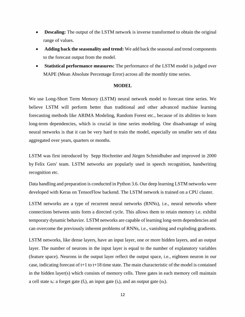
LSTM networks, like dense layers, have an input layer, one or more hidden layers, and an output

layer. The number of neurons in the input layer is equal to the number of explanatory variables

(feature space). Neurons in the output layer reflect the output space, i.e., eighteen neuron in our

case, indicating forecast of t+1 to t+18 time state. The main characteristic of the model is contained

in the hidden layer(s) which consists of memory cells. Three gates in each memory cell maintain

a cell state st: a forget gate (ft), an input gate (it), and an output gate (ot).

13

The structure of the memory cell is illustrated in Fig. 6 below.

Figure 6: LSTM model's memory cell architecture (As illustrated in NVIDIA Developer Blog-Deep Learning in a Nutshell: Sequence Learning by Tim Dettmers on March 7, 2016)

• Forget gate: Defines which information is removed from the cell state.

• Input gate: Specifies which information is added to the cell state.

• Output gate: Specifies which information from the cell state is used as output.

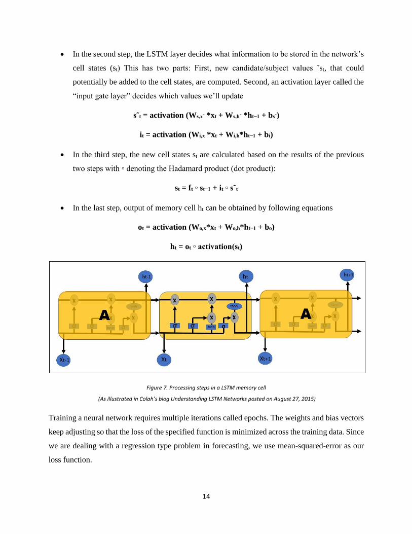
As illustrated in Fig. 7 at every timestep t, each gate is presented with the current input xt. and the

output ht-1 of the memory cells at the previous timestep t − 1. Each gate has a bias vector associated

with it which adds to its calculated value after every input. The working of an LSTM layer can be

summarized in the following steps:

• In the first step, the LSTM layer generates activation values of its forget gates at timestep

t, based on current input xt, previous timestep output ht and the bias term associated with

the gates. This determines the information to be removed from its previous cell states st-1.

An ‘activation’ function (sigmoid always here) finally scales all the values into a suitable

normalized range which determines varying degree of forgetfulness of the input:

ft = activation (Wf,x*xt + Wf,h*ht−1 + bf )

14

• In the second step, the LSTM layer decides what information to be stored in the network’s

cell states (st) This has two parts: First, new candidate/subject values ˜st, that could

potentially be added to the cell states, are computed. Second, an activation layer called the

“input gate layer” decides which values we’ll update

s˜t = activation (Ws,x˜ *xt + Ws,h˜ *ht−1 + bs˜)

it = activation (Wi,x *xt + Wi,h*ht−1 + bi)

• In the third step, the new cell states st are calculated based on the results of the previous

two steps with ◦ denoting the Hadamard product (dot product):

st = ft ◦ st−1 + it ◦ s˜t

• In the last step, output of memory cell ht can be obtained by following equations

ot = activation (Wo,x*xt + Wo,h*ht−1 + bo)

ht = ot ◦ activation(st)

Figure 7. Processing steps in a LSTM memory cell

(As illustrated in Colah’s blog Understanding LSTM Networks posted on August 27, 2015)

Training a neural network requires multiple iterations called epochs. The weights and bias vectors

keep adjusting so that the loss of the specified function is minimized across the training data. Since

we are dealing with a regression type problem in forecasting, we use mean-squared-error as our

loss function.

15

In our case, we make use of Adam optimizer (commonly used), as optimizer via keras for the

training of the LSTM network. The specified topology of our trained LSTM network is hence as

follows:

• Input layer with one feature and six timesteps.

• LSTM layer with h = 20 hidden neurons and ‘relu’ activation function.

• Output layer (dense layer) with 18 neurons.

RESULTS

Our dataset consists of more than 1428 univariate time-series aggregated over monthly frequency

level. We have built LSTM models for each time-series and forecasted values (quantity demanded)

for next eighteen timesteps. However, for purpose of this paper, we present through graphical

visualization few examples of time series randomly chosen from our dataset. We then contrast our

LSTM model against feed-forward neural networks and theta decomposed exponential smoothing

model (winner of M3 Competition).

We select MSE (Mean Squared Error) to train our networks and MAPE (Mean Absolute

Percentage Error) as our performance measure against the test set. We choose MAPE because

different time series have a different range of values, hence errors in percentage terms help in

relative comparisons among a different set of time series. The plot of prediction on the validation

dataset is shown below:

16

On running the LSTM model for 1428 time series, we observe most MAPE values between 4%

to 35% with the average being around 20%.

Figure 8: Plot of monthly aggregated time series and forecast

We further compared these results against other models as mentioned above. The feed-forward

neural networks model gives an average of 19%, but it requires a lot of feature engineering. LSTM

model performs better than traditional exponential smoothing model which gives MAPE average

of about 21%. An additional advantage of LSTM model over traditional models is that it requires

lot less data preprocessing and can be automated without visualizing the number of lags required

to be included for prediction.

CONCLUSION

Inventory management is no longer just any task performed by those in the purchase department/

warehouse function but is now at the core of operational performance in most industries.

Companies are investing heavily to ensure they get the optimum level of inventory at any point in

time to minimize overhead costs and maximize revenues. However, organizations are still far from

understanding to what extent descriptions, prescriptions, and predictions of these models are valid

in the industry to give companies a competitive advantage.

17

The objective of this study was to try and develop one such model using a Recurrent Neural

Network to forecast demand that offsets the disadvantages of traditional demand prediction

models. The data used was from a publicly available source and represents various fields such as

Finance, Economics, Demographics etc. The baseline models tested by the clients were Feed

Forward Neural Network and Exponential Smoothing. In the study, Long-Short Term Memory

Network was trained and tested on monthly level time series data. It was observed that LSTM

Neural Network model performs better (lower MAPE) than the baseline models and requires

minimal feature engineering.

We believe this study could be a valuable contribution in the area efficient demand prediction

and inventory management enabling enhanced cost savings. LSTM Neural Network has the

ability to take into consideration long-term dependencies and eliminates the need to visualize the

number of relevant demand lags to be fed into the model. LSTM can be considered a successful

decision support tool in demand forecasting in the Supply Chain and Logistics industry as well

as other industries.

REFERENCES

Hochreiter Sepp, Sehmidhuber Jurgen (1997) “Long Short-Term Memory”

Gers Felix A., Sehmidhuber Jurgen, Cummins Fred (1999) “Learning to Forget: Continual

Prediction with LSTM”

Patterson Josh, Gibson Adam (2017), “Deep Learning: A Practitioner’s Approach”

Abdelhadi Azzouni,Guy Pujolle (2009) “A Long Short-Term Memory Recurrent Neural

Network Framework for Network Traffic Matrix Prediction”

Bonnes Kevin (2015),“Predictive Analytics for Supply Chains: A Systematic Literature

Review”

C. W. J. Granger and M. J. Morris (1976),” Time Series Modelling and Interpretation”

Durga Toshniwal , R. C. Joshi(2012)“Result of Research: Using Cumulative Weighted Slopes

for Clustering Time Series Data”

18

Fischer, Thomas Krauss Christoper (2017)“Deep learning with long short-term memory

networks for financial market predictions”

Ian Goodfellow, Yoshua Bengio, Aaron Courville (2009),” Deep Learning”

James Hamilton (1995), “A New Approach to the Economic Analysis of Nonstationary Time

Series and the Business Cycle”

Jan G. De Gooijer, Kuldeep Kumar “Some recent developments in non-linear time series

modeling, testing, and forecasting”

JW Taylor (2003) “Short-term electricity demand forecasting using double seasonal

exponential smoothing”

Kanad Chakroborthy, Kishan Malhotra, Chilikuri Mohan (1992), “Forecasting the behavior of

multivariate time series using neural networks”

M.Langvist, L. Karlsson, A Loufti (2014) “A review of unsupervised feature learning and deep

learning for time-series modeling”

Rob J Hyndman, George Athanasopoulos (2008), “Forecasting Principles and Practice”

S Makridakis, A Andersen, R Carborne, R Fildes (1982) “The accuracy of extrapolation (time

series) methods: Results of a forecasting competition”

Yuehui Chen, Bo Yang, Jiwen Dong, Ajith Abraham (2005), “Time-series forecasting using

flexible neural tree model”