A solver for Boussinesq shallow water equations · A solver for Boussinesq shallow water equations...

The Boussinesq models Numerical model Tutorial setup Results and discussion

A solver for Boussinesqshallow water equations

Dimitrios Koukounas

Department of Mechanics and Maritime sciencesChalmers University of Technology,

Gothenburg, Sweden

2017-11-23

Dimitrios Koukounas Beamer slides template 2017-11-23 1 / 30


Shallow water waves

Characteristics of a shallow water wave

Wavelength larger or much larger than the depth O( ld) > 1, usually

O( ld) >> 1

Varying dispersion with respect to depth

Very shallow water limit of propagation velocity√gh0

Non linear terms of the surface and bottom BCs become important



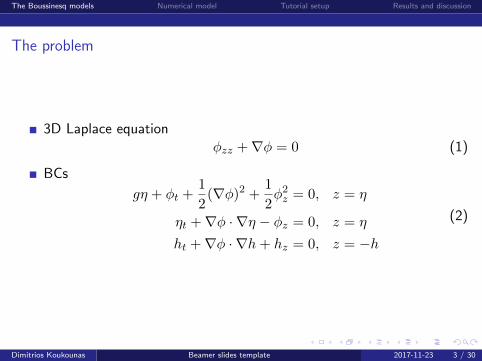
The problem

3D Laplace equationφzz +∇φ = 0 (1)

BCs

gη + φt +1

2(∇φ)2 + 1

2φ2z = 0, z = η

ηt +∇φ · ∇η − φz = 0, z = η

ht +∇φ · ∇h+ hz = 0, z = −h

(2)



The problem

Making non dimensional

(x, y) = κ0(x, y), η =η

α0, z =

z

h0, h =

h

h0

t = (κ0gh0)t, φ = (α0

κ0h0

√gh0)

−1φ

3D Laplace equationφzz + µ2∇φ = 0 (3)



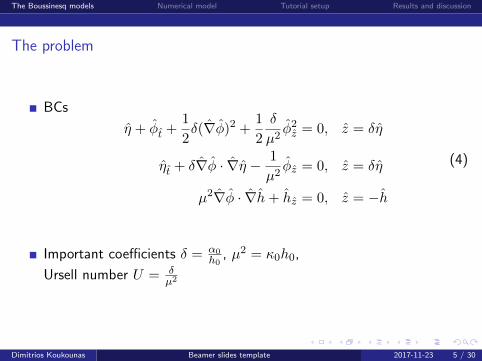
The problem

BCs

η + φt +1

2δ(∇φ)2 + 1

2

δ

µ2φ2z = 0, z = δη

ηt + δ∇φ · ∇η − 1

µ2φz = 0, z = δη

µ2∇φ · ∇h+ hz = 0, z = −h

(4)

Important coefficients δ = α0h0

, µ2 = κ0h0,

Ursell number U = δµ2



Why Boussinesq?

Airy’s fully non linear SWM is unrestricted in nonlinearity but doesn’taccount for dispersion

Boussinesq model introduces dispersion

Key assumptions:

Long wave approach

moderate non linearity

dispersion as important as nonlinearity O(U) ' 1



The standard Boussinesq model

By setting B = 0 we obtain the Abbott model

By setting B = 115 we obtain the Madsen-Sorrensen equations

u(x, y, t) is the depth averaged velocity

ut+u·∇u+g∇η =h

2∇∇·(hut)+(Bh2−h

2

6)∇∇·ut+Bh2g∇(∇2η) (5)

ηt = −∇[(h+ η)u] (6)



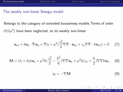
The weakly non-linear Nwogu model

Belongs to the category of extended boussinesq models Terms of order

O(δµ2) have been neglected, so its weakly non-linear

uat + δua · ∇ua +∇η + µ2(z2a2∇∇ · uat + za∇∇ · huat) = 0 (7)

M = (h+ δη)ua + µ2h(z2a2− h2

6)∇∇ua + µ2h(za +

h

2)∇∇hua (8)

ηt = −∇M (9)



The NwoguFoamRK solver

Main features of the solver

In this project constant depth is assumed for simplicity

A 4th order Runge Kutta time integration scheme is implemented

Inside the RK loop, two functions are called to calculate the timederivatives of η and ua respectively

The solver interacts with 3 fields, namely eta, Ua and Uat



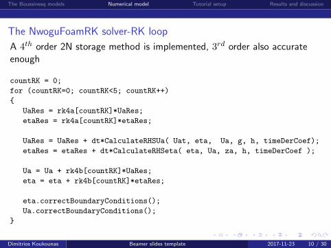
The NwoguFoamRK solver-RK loop

A 4th order 2N storage method is implemented, 3rd order also accurateenough

countRK = 0;

for (countRK=0; countRK<5; countRK++)

{

UaRes = rk4a[countRK]*UaRes;

etaRes = rk4a[countRK]*etaRes;

UaRes = UaRes + dt*CalculateRHSUa( Uat, eta, Ua, g, h, timeDerCoef);

etaRes = etaRes + dt*CalculateRHSeta( eta, Ua, za, h, timeDerCoef );

Ua = Ua + rk4b[countRK]*UaRes;

eta = eta + rk4b[countRK]*etaRes;

eta.correctBoundaryConditions();

Ua.correctBoundaryConditions();

}



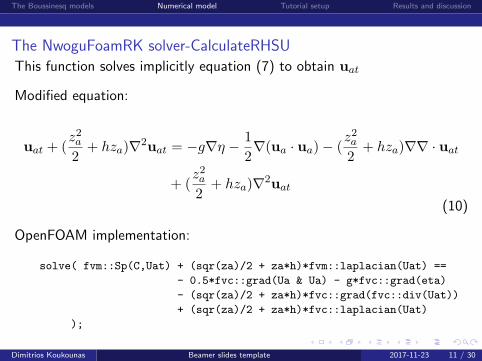
The NwoguFoamRK solver-CalculateRHSU

This function solves implicitly equation (7) to obtain uat

Modified equation:

uat + (z2a2

+ hza)∇2uat = −g∇η −1

2∇(ua · ua)− (

z2a2

+ hza)∇∇ · uat

+ (z2a2

+ hza)∇2uat

(10)

OpenFOAM implementation:

solve( fvm::Sp(C,Uat) + (sqr(za)/2 + za*h)*fvm::laplacian(Uat) ==

- 0.5*fvc::grad(Ua & Ua) - g*fvc::grad(eta)

- (sqr(za)/2 + za*h)*fvc::grad(fvc::div(Uat))

+ (sqr(za)/2 + za*h)*fvc::laplacian(Uat)

);



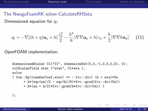
The NwoguFoamRK solver-CalculateRHSeta

Dimensioned equation for ηt:

ηt = −∇[(h+ η)ua + h(z2a2− h2

6)∇∇ua + h(za +

h

2)∇∇hua] (11)


dimensionedScalar C1("C1", dimensionSet(0,0,-1,0,0,0,0), 0);

volScalarField etat ("etat", C1*eta );

solve

( fvm::Sp(timeDerCoef,etat) == - fvc::div( (h + eta)*Ua

+ h*(sqr(za)/2 - sqr(h)/6)*fvc::grad(fvc::div(Ua))

+ h*(za + h/2)*fvc::grad(h*fvc::div(Ua)) )

);



The AbbottRK solver-CalculateRHSU

This function solves implicitly equation (5) to obtain ut

NOTE: The same notion Ua is also used in the implementation of theAbbott solver to describe the velocity variable u

ut − (B +1

3)h2∇2ut = −g∇η −

1

2∇(u · u) + (B +

1

3)h2∇∇ · ut

− (B +1

3)h2∇2ut +Bgh2∇(∇2η)

(12)


solve( fvm::Sp(C,Uat) - (B+(1.0/3.0))*sqr(h)*fvm::laplacian(Uat) ==

- 0.5*fvc::grad(Ua & Ua) - g*fvc::grad(eta)

+ (B+(1.0/3.0))*sqr(h)*fvc::grad(fvc::div(Uat))

- (B+(1.0/3.0))*sqr(h)*fvc::laplacian(Uat)

+B*g*sqr(h)*fvc::grad( fvc::laplacian(eta) )

);



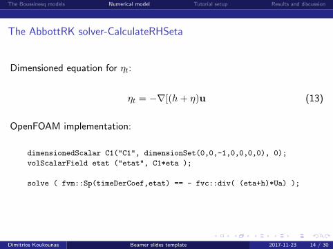
The AbbottRK solver-CalculateRHSeta

Dimensioned equation for ηt:

ηt = −∇[(h+ η)u (13)


dimensionedScalar C1("C1", dimensionSet(0,0,-1,0,0,0,0), 0);

volScalarField etat ("etat", C1*eta );

solve ( fvm::Sp(timeDerCoef,etat) == - fvc::div( (eta+h)*Ua) );



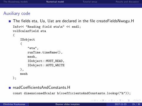
Auxiliary code

The fields eta, Ua, Uat are declared in the file createFieldsNwogu.H

Info<< "Reading field eta\n" << endl;

volScalarField eta

(

IOobject

(

"eta",

runTime.timeName(),

mesh,

IOobject::MUST_READ,

IOobject::AUTO_WRITE

),

mesh

);

readCoefficientsAndConstants.H

const dimensionedScalar h(coefficientsAndConstants.lookup("h"));



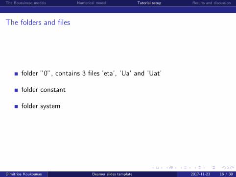
The folders and files

folder ”0”, contains 3 files ’eta’, ’Ua’ and ’Uat’

folder constant

folder system



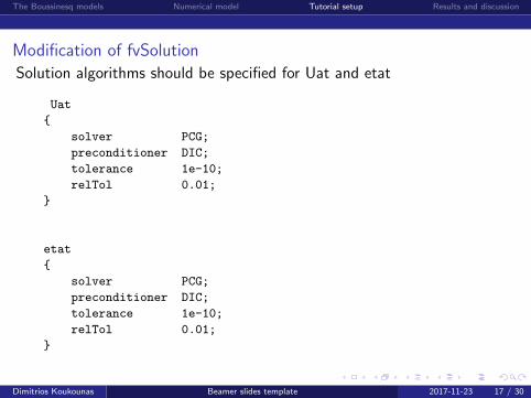
Modification of fvSolution

Solution algorithms should be specified for Uat and etat

Uat

{

solver PCG;

preconditioner DIC;

tolerance 1e-10;

relTol 0.01;

}

etat

{

solver PCG;

preconditioner DIC;

tolerance 1e-10;

relTol 0.01;

}



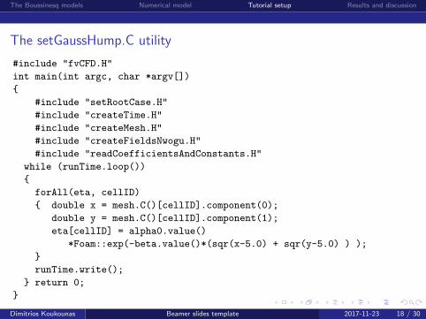
The setGaussHump.C utility

#include "fvCFD.H"

int main(int argc, char *argv[])

{

#include "setRootCase.H"

#include "createTime.H"

#include "createMesh.H"

#include "createFieldsNwogu.H"

#include "readCoefficientsAndConstants.H"

while (runTime.loop())

{

forAll(eta, cellID)

{ double x = mesh.C()[cellID].component(0);

double y = mesh.C()[cellID].component(1);

eta[cellID] = alpha0.value()

*Foam::exp(-beta.value()*(sqr(x-5.0) + sqr(y-5.0) ) );

}

runTime.write();

} return 0;

}



Boundary Conditions and parameters of the analysis

slip boundary condition for the velocity Ua

zeroGradient for eta

depth h = 0.5 m

length x breadth = 10 m x 10 m

gaussian hump initial max 0.1 m

shape parameter beta = 0.4

g = 9.81 m/s2



Running the tutorial

Steps

Run the blockMeshDict

Specify the desired values for alpha0 and beta of the gaussian hump

In controlDict set: startTime 0, endTime 1, deltaT 1, writeInterval 1

Run the setGaussHump utility

Delete the folder ”0” and rename the folder ”1” to ”0”

Reset the controlDict parameters to the desired values

Run the tutorial



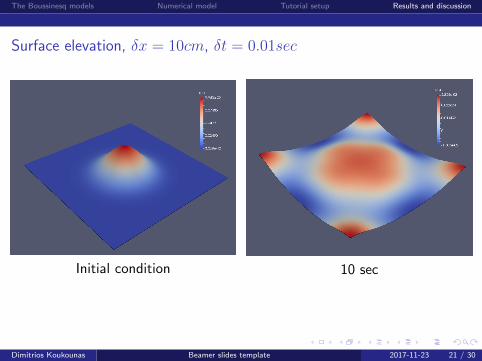
Surface elevation, δx = 10cm, δt = 0.01sec

Initial condition 10 sec



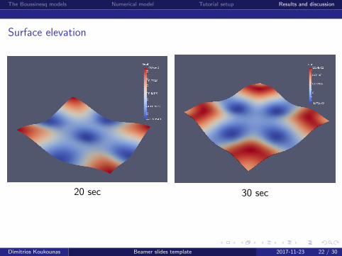
Surface elevation

20 sec 30 sec



Surface elevation

40 sec 50 sec



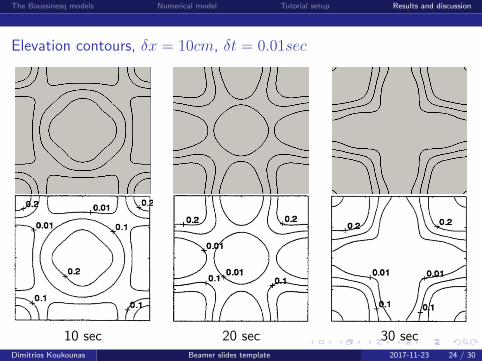
Elevation contours, δx = 10cm, δt = 0.01sec

10 sec 20 sec 30 secDimitrios Koukounas Beamer slides template 2017-11-23 24 / 30


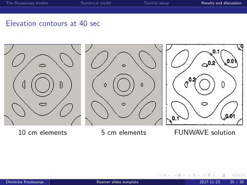
Elevation contours at 40 sec

10 cm elements 5 cm elements FUNWAVE solution



Elevation contours at 50 sec

10cm elements 5 cm elements FUNWAVE solution



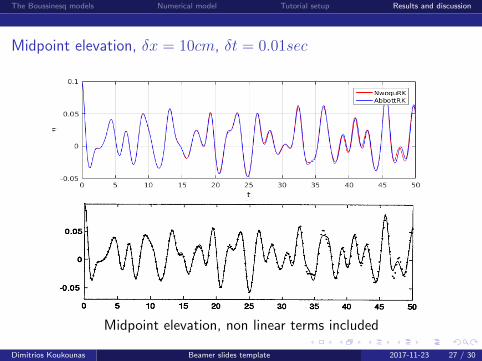
Midpoint elevation, δx = 10cm, δt = 0.01sec

Midpoint elevation, non linear terms included



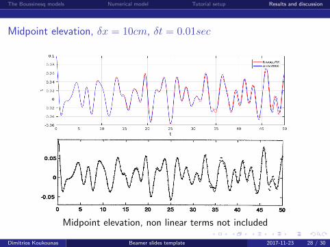
Midpoint elevation, δx = 10cm, δt = 0.01sec

Midpoint elevation, non linear terms not included



Future work

Study of slightly alternative implementation of the Runge Kuttascheme

Study of the plane wave propagation

Study of soliton propagation



That’s it

Thank you for your attention!


Date post:	26-Apr-2018
Category:	Documents
Upload:	lexuyen
View:	231 times
Download:	3 times

A solver for Boussinesq shallow water equations · A solver for Boussinesq shallow water equations...

Documents