A Sparse Manifold Classification Method Based on a Multi ...

International Journal of

Geo-Information

Article

A Sparse Manifold Classification Method Based ona Multi-Dimensional Descriptive Primitive ofPolarimetric SAR Image Time Series

Chu He 1,2,*, Gong Han 1 , Di Feng 1, Juan Du 3,* and Mingsheng Liao 2

1 Signal Processing Laboratory, Electronic Information School, Wuhan University, Wuhan 430072, China;[email protected] (G.H.); [email protected] (D.F.)

2 State Key Laboratory for Information Engineering in Surveying, Mapping and Remote Sensing,Wuhan University, Wuhan 430079, China; [email protected]

3 Remote Sensing and Information Engineering School, Wuhan University, Wuhan 430079, China* Correspondence: [email protected] (C.H.); [email protected] (J.D.);

Tel.: +86-133-0716-2028 (C.H.); +86-186-0272-0952 (J.D.)

Academic Editor: Wolfgang KainzReceived: 18 January 2017; Accepted: 25 March 2017; Published: 29 March 2017

Abstract: Classification using the rich information provided by time-series and polarimetric SyntheticAperture Radar (SAR) images has attracted much attention. The key point is to effectively revealthe correlation between different dimensions of information and form a joint feature. In this paper,a multi-dimensional SAR descriptive primitive for each single pixel is firstly constructed, which inthe polarimetric scale obtains incoherent information through target decompositions while in thetime scale obtains coherent information through stochastic walk. Secondly, for the purpose of featureextraction and dimension reduction, a special feature space mapping for the descriptive primitive ofthe whole image is proposed based on sparse manifold expression and compressed sensing. Finally,the above feature is inputted into a support vector machine (SVM) classifier. This proposed methodcan inherently integrate the features of polarimetric SAR times series. Experiment results on three realtime-series polarimetric SAR data sets show the effectiveness of our presented approach. The idea ofa multi-dimensional descriptive primitive as a convenient tool also opens a new spectrum of potentialfor further processing of polarimetric SAR image time series.

Keywords: polarimetric SAR time series; image classification; multi-dimensional descriptiveprimitive; sparse manifold expression; compressed sensing

1. Introduction

Synthetic aperture radar (SAR) can be used in a vast majority of application areas due to its abilityto work day and night under all weather conditions. However, its coherent imaging mechanism andextremely low signal-to-noise ratio make it difficult to interpret. In recent years, increasing accessof polarimetric and time-series SAR data has provided abundant information regarding the specificlocation. However, how to fully utilize this information has emerged as a basic problem in SAR imageinterpretation.

With respect to the incoherent information from a single SAR image, quite a few product statisticalmodel distributions have been proposed for classification. Classical ones include the earliest Gammadistribution, K distribution, G0 distribution and G distribution [1]. Note that the use of polarimetryfor radar remote sensing is increasingly extensive; a set of methods known collectively as targetdecomposition (TD) theorems springs up, which were first formalized by Huynen [2] but have theirroots in the work of Chandrasekhar on light scattering by small anisotropic particles [3]. Since this

ISPRS Int. J. Geo-Inf. 2017, 6, 97; doi:10.3390/ijgi6040097 www.mdpi.com/journal/ijgi

http://www.mdpi.com/journal/ijgi

http://www.mdpi.com

http://www.mdpi.com/journal/ijgi

ISPRS Int. J. Geo-Inf. 2017, 6, 97 2 of 12

original work, there have been many other effective decompositions such as Cloude decomposition,Holm decomposition, Krogager decomposition and Huynen decomposition [4].

As for the coherent information from multiple images, time-series SAR provides the possibilityof extracting the interference information. By unwrapping the achieved information, the elevationinformation and structure information of the ground can be obtained. Representative instances areBranch-Cut Algorithm, Minimum Discontinuity, Mask-Cut Algorithm and Minimum Lp-Norm PhaseUnwrapping [5].

With this incoherent and coherent information, researchers have developed various imageprocessing patterns for SAR classification from the combination of polarimetric distribution andclassifiers [6] to the combination of extracted features and classifiers [7] and nowadays to deeplearning [8]. Applicable to all patterns, a promising direction is to optimally relate the incoherentinformation together with the coherent information.

So far, many feature-fusing methods have been proposed. Here, we introduce three kinds ofprocessing sketches: co-training, multiple kernel learning and subspace learning [9–12]. Duringeach iteration of Co-training [13], models are trained separately but relative to each feature and thenthe algorithm propagates the disagreement of the two models back to the training set. In multiplekernel learning methods, each feature corresponds to a kernel which best matches its property andthen these kernels are simultaneously connected in a linear or nonlinear way. One representativemultiple kernel learning algorithm is Simple MKL which combines kernels linearly and sparsely [14].Subspace learning aims at finding the shared underlying subspace on the assumption that the originalfeatures are generated from this latent subspace by a specific mapping. Principle Components Analysis(PCA) [15] is a time-honored and simple technique performing subspace learning. Figure 1 sketchesthe three processing approaches.

feature 1 feature 2

model 1 model 2

predict predictsame

validation set

linear/

nonlinear

train set

validation set validation set

space 1 space 2

subspace

co-training multiple kernel learning subspace learning

Figure 1. Sketches of co-training, multiple kernel learning and subspace learning.

However, the involvement of unwrapping and the complexity of the InSAR inverse procedurecomplicate the process of accurate height inversion for classification, making how to obtain coherentinformation without unwrapping and inversion a critical issue. Worse still, neither co-training, normultiple kernel learning nor subspace learning merge features at the initial feature construction stage.In this framework, we are dedicated to exploring a rather concise approach which can also inherentlyintegrate the features of polarimetric SAR times series.


The main contributions of our work are two-fold. Firstly a multi-dimensional SAR descriptiveprimitive for each single pixel is constructed, which in the polarimetric scale obtains incoherentinformation, while in the time scale obtains coherent information. The descriptive primitive can becomea convenient tool for the processing of polarimetric SAR image time series. Secondly, consideringthe inconsistency between polarimetric incoherent scale and time-series coherent scale, a nonlinearclassification model is further constructed based on sparse manifold expression and compressedsensing for feature extraction and dimension reduction. This model can deal with the inconsistencyof the two scales and tactfully avoid the nonlinearity problem brought by the multiplicative modelof SAR.

The rest of the paper is organized as follows. Section 2 is dedicated to the creation of amulti-dimensional descriptive primitive. Section 3 introduces the sparse manifold classificationmodel. Section 4 shows the validations on three real polarimetric SAR data sets. The conclusion isincluded in Section 5.

2. The Multi-Dimensional Descriptive Primitive

2.1. Incoherent Feature in the Polarization Scale

In the polarimetric scale, target decompositions are taken advantages of to generateincoherent information of every single SAR image, which include Pauli decomposition,SDH decomposition, Huynen decomposition, Holm decomposition and Cloude decomposition in thispaper. Every decomposition creates three parameters for a single pixel. We bunch together all theseparameters generated by these five decompositions into a 5× 3 matrix.

2.2. Coherent Feature in the Time Scale

In the time scale, stochastic walk is utilized to form the coherent feature of the time-series data.Stochastic walk was first used by Francisco Estrada et al. for image denoising [16]. Its simple conceptis set on the basis of random walk probabilities. Every random walk, beginning from a given pixel,paths smoothly over arbitrary surrounding neighborhoods. The random walk probability betweenpaired pixels is determined by their similarity, which serves as a weight.

Define an ordered pixel sequence T0,k = x0, x1, . . . , xk to represent a path from x0 to xk.The transition probability between two consecutive pixels xj and xj+1 within this sequence is inverselyproportional to both the dissimilarity between xj and xj+1 and the dissimilarity between x0 andxj+1 [16], which is expressed by Equation (1).

p(

xj+1 | xj)=

1K

e−d(x0,xj+1)

2

2δ2 e−d(xj ,xj+1)

2

2δ2 (1)

Here, K is a parameter for normalization and δ is for scaling. d(xi, xj

)is a dissimilarity measure

relating image pixel xi and xj. According to the first-order Markov assumption, the probability ofthe whole sequence is accessible. With T0,k in hand, T0,k+1 can be directly created by generating theneighborhood of xk and then selecting a neighbor with probability p (xk+1 | xk). If m random walksare given and each is originating from x0 with a length of k steps, the final result shall be calculated asthe weighted mean of all pixels visited in every step during every walk.

In the proposed method, the original 2-D neighborhood is expanded into a 3-D one.The neighborhood of a specific pixel in time t consists of not only the eight pixels surroundingit but also the 18 pixels in adjacent time t− 1 and t + 1.

2.3. Multi-Dimensional Descriptive Primitive

In registered polarimetric SAR images, each single pixel has its corresponding polarimetricmatrix T. Firstly, extract all the 3× 3 matrix T of a same point on different dates and connect all


the matrixes together according to the time sequence. This is a prototype of our multi-dimensionaldescriptive primitive. On this primitive, we implement target decompositions in the polarimetric scaleand then stochastic walk in the time scale, thus integrating the incoherent feature with the coherentfeature to get our multi-dimensional descriptive primitive of a single point. In our work, we selectedthree discrete dates to generate a 3-D descriptive primitive which is shown in Figure 2. The three3× 3 matrix T of the same point on different dates, together, made up a three-dimensional cube, whichwas the raw material of the subsequent processes. In the polarimetric scale, each 3× 3 matrix T wasdealt with 5 target decompositions. With every decomposition generating 3 parameters, three 3× 3matrix T were transformed into three 5× 3 incoherent feature matrixes, constructing a primitive withonly incoherent feature. In the time scale, stochastic walk was utilized on the three 5× 3 matrixes toupdate the incoherent feature primitive with the coherent feature. Then, all the bases were connectedtogether to generate a three-dimensional descriptive primitive of a whole graph.

time scale

polar scale

t-1 t t+1

Pt-1 Pt Pt+1

target

decompositions

stochastic walk

Tt-1 Tt Tt+1

t t+1t-1

SDH

Huynen

Holm

Cloude

Pauli

Tt-1 Tt Tt+1

Figure 2. A 3-D descriptive primitive of a single point.

3. The Sparse Manifold Classification Model

When the size of the involved SAR image is relatively big, the problem may occur that thedescriptive primitive is too large for the subsequent operations. Besides, the problem of the nonlinearitymultiplicative model brought by the coherent imaging mechanism of SAR calls for an adaptableapproach. To these ends, we propose a nonlinear classification model based on sparse manifoldexpression and compressed sensing.

3.1. Sparse Manifold Expression

Sparse representation has always been an effective feature extraction approach in the classificationarea. Existing sparse coding models linearly assemble the basic atoms in an over-complete dictionaryto approximate the input signal. Assuming that xi is the d dimensional local feature of the SARimage, i.e., X = [x1, . . . , xN ] ∈ Rd×N and B = [b1, . . . , bM] ∈ Rd×M is the dictionary with Mentries, every input can be represented by its most similar M-dimensional code ωi which satisfiesxi = Bωi. Ω = [ω1, . . . , ωN ] is the set of the codes. Taking the Locality-constrained Linear Coding(LLC) model [17] as an example, we can break it into two parts, the first of which is a coding error termand captures typical features of local description; the second part constraints the code to make surethat the under-determined system of the equation has a unique solution. The following expressiongives the details.

argminΩ

N

∑i=1‖xi − Bωi‖2 + λ‖di ·ωi‖2 s.t. 1Twi = 1, ∀i (2)

λ is a constraint parameter and “·” denotes the multiplication in element-wise. di ∈ RM

represents the locality adaptor to maintain the similarity between the base vector and the input


descriptor, which is usually normalized to be between (0, 1]. The constraint 1Twi = 1 guaranteesthe shift-invariant requirements of the LLC code. Though the LLC model performs well in mostsituations, it is not applicable to nonlinear cases. In our context, to better integrate the polarimetricscale and the time-series scale and to handle the nonlinearity of the SAR multiplicative model, webring in sparse manifold expression to find the potential low dimensional structure in the featurespace. Manifold learning supposes that points in a high dimensional space virtually exist in a lowdimensional manifold. Inspired by Locally Linear Embedding (LLE) [18], we resort to a manifold bypreserving the neighborhood in the original data space and then mapping the data into global internalcoordinates on this manifold while keeping the local geometry unchanged. The data descriptor withthe form of a 3-D primitive in this paper is no longer x ∈ Rd but x′ ∈ R5×3×t. t is the number ofdifferent dates in the time-series data set. In our experiments, each data set has three different dates,i.e., t = 3. We reconstruct each x′ from its neighbors by linear coefficients γi,j in Equation (3) andthen fix the coefficients to optimize yi in the low-dimensional manifold which corresponds to x′ inEquation (4).

argminΓ

∑i‖x′i −∑

jγi,jx′j‖2 s.t. ∑

jγi,j = 1 (3)

argminY

∑i‖yi −∑

jγi,jyj‖2 (4)

Here Y = [y1, . . . , yN ] ∈ R3×1×t×N . The manifold perspective takes into account the inconsistencybetween polarimetric scale and time scale. Besides, the intrinsic distribution of data is also explored.Thus, both characteristics of the incoherent feature and coherent feature can be looked after well.Let C = [c1, . . . , cM] ∈ R3×1×t×M be the dictionary. θi is the corresponding code for yi. Plug yi intoEquation (2) to get the following sparse manifold expression:

argminΘ

N

∑i=1‖yi − Cθi‖2 + λ‖di · θi‖2 s.t. 1Tθi = 1, ∀i (5)

3.2. Compressed Sensing

The construction of the required over-complete dictionary is complex and the sparse featureremains redundant, which yields the performance in some degree. An ideal output code requireslow-dimension preservation and high-information retention. For this purpose, we further optimizethe sparse priors in Equation (5) with the aim of reducing the signal’s dimension by introducinga matrix A in Equation (6).

argminΘ

N

∑i=1‖Ayi − Cθi‖2 + λ‖di · θi‖2 s.t. 1Tθi = 1, ∀i (6)

The compressed sensing [19] method captures and represents compressible signals at a ratesignificantly below the Nyquist rate. Our presented method takes advantage of compressed sensing forbetter feature extraction and dimension reduction. The input feature Y is projected into a wavelet base ϕ.The corresponding coefficients α = ϕTY are found to contain few large values and many small values.So a random Gaussian matrix Φ is introduced to act as an observation matrix for its inconsistency withwavelet basis, i.e., Z = Φα. This randomness cannot guarantee that the reconstructed feature coding isthe sparsest one. Thus, further constraints and optimizations are made in Equation (7).

argminD,Θ

N

∑i=1‖zi − Dθi‖2 + λ‖di · θi‖2 s.t. ‖dj‖ ≤ 1, | di,j ≥ ξ ∀j = 1, . . . , d, i = 1, . . . , N (7)

Here D = ΦϕT . The 2-norm constraint on vector di helps to avoid trivial solutions and theconstraint on di,j helps to obtain prominent dictionary atoms.


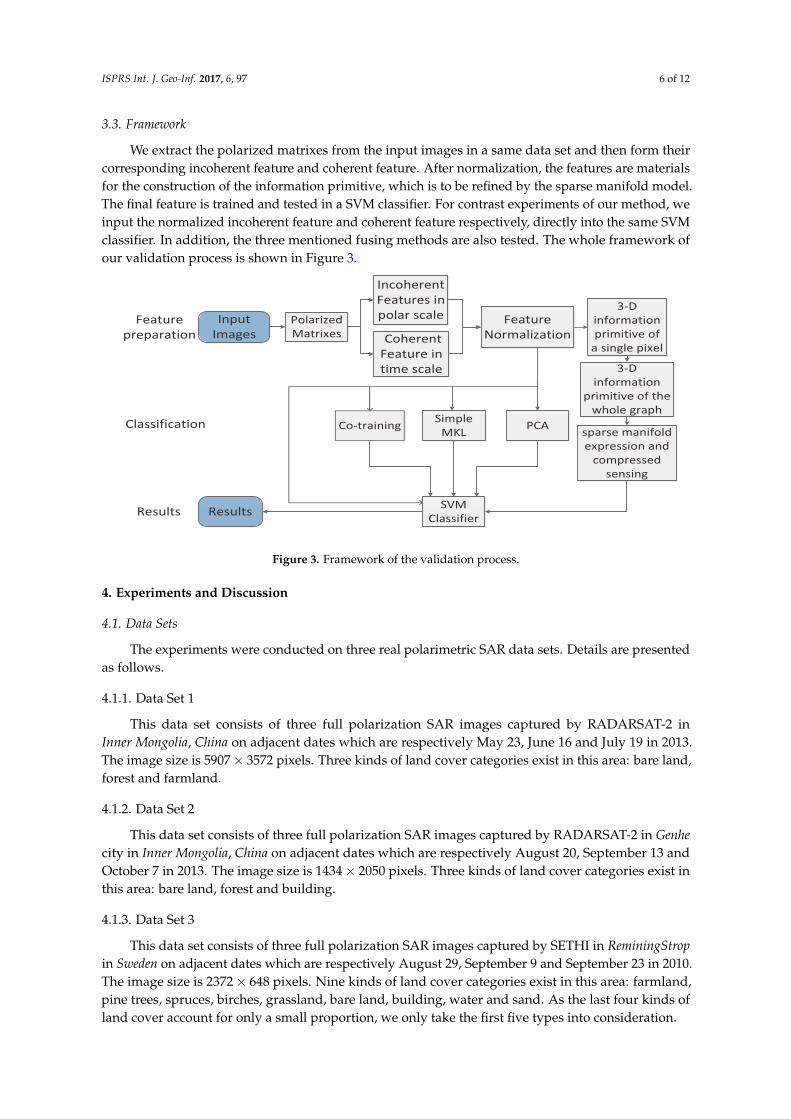
3.3. Framework

We extract the polarized matrixes from the input images in a same data set and then form theircorresponding incoherent feature and coherent feature. After normalization, the features are materialsfor the construction of the information primitive, which is to be refined by the sparse manifold model.The final feature is trained and tested in a SVM classifier. For contrast experiments of our method, weinput the normalized incoherent feature and coherent feature respectively, directly into the same SVMclassifier. In addition, the three mentioned fusing methods are also tested. The whole framework ofour validation process is shown in Figure 3.

Input

Images

Polarized

Matrixes

Incoherent

Features in

polar scale

Coherent

Feature in

time scale

Feature

Normalization

Co-trainingSimple

MKLPCA

3-D

information

primitive of

a single pixel

3-D

information

primitive of the

whole graph

sparse manifold

expression and

compressed

sensing

SVM

ClassifierResults

Feature

preparation

Classification

Results

Figure 3. Framework of the validation process.

4. Experiments and Discussion

4.1. Data Sets

The experiments were conducted on three real polarimetric SAR data sets. Details are presentedas follows.

4.1.1. Data Set 1

This data set consists of three full polarization SAR images captured by RADARSAT-2 inInner Mongolia, China on adjacent dates which are respectively May 23, June 16 and July 19 in 2013.The image size is 5907× 3572 pixels. Three kinds of land cover categories exist in this area: bare land,forest and farmland.

4.1.2. Data Set 2

This data set consists of three full polarization SAR images captured by RADARSAT-2 in Genhecity in Inner Mongolia, China on adjacent dates which are respectively August 20, September 13 andOctober 7 in 2013. The image size is 1434× 2050 pixels. Three kinds of land cover categories exist inthis area: bare land, forest and building.

4.1.3. Data Set 3

This data set consists of three full polarization SAR images captured by SETHI in ReminingStropin Sweden on adjacent dates which are respectively August 29, September 9 and September 23 in 2010.The image size is 2372× 648 pixels. Nine kinds of land cover categories exist in this area: farmland,pine trees, spruces, birches, grassland, bare land, building, water and sand. As the last four kinds ofland cover account for only a small proportion, we only take the first five types into consideration.


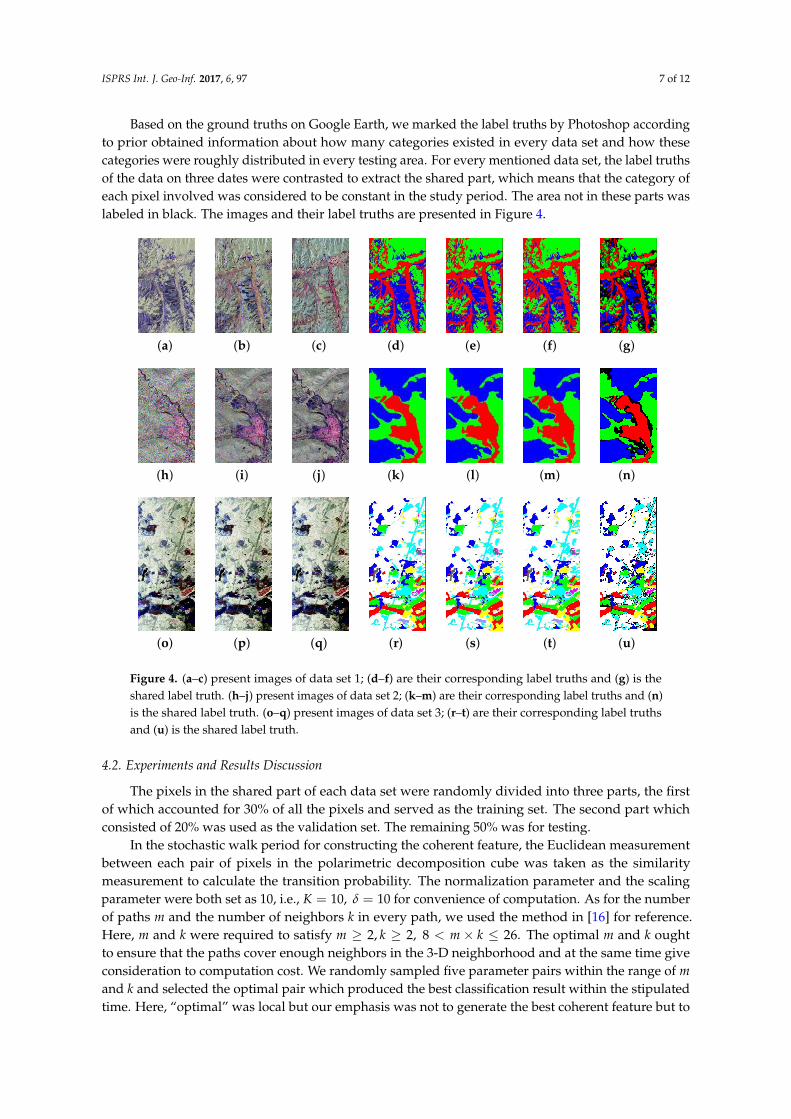
Based on the ground truths on Google Earth, we marked the label truths by Photoshop accordingto prior obtained information about how many categories existed in every data set and how thesecategories were roughly distributed in every testing area. For every mentioned data set, the label truthsof the data on three dates were contrasted to extract the shared part, which means that the category ofeach pixel involved was considered to be constant in the study period. The area not in these parts waslabeled in black. The images and their label truths are presented in Figure 4.

(a) (b) (c) (d) (e) (f) (g)

(h) (i) (j) (k) (l) (m) (n)

(o) (p) (q) (r) (s) (t) (u)

Figure 4. (a–c) present images of data set 1; (d–f) are their corresponding label truths and (g) is theshared label truth. (h–j) present images of data set 2; (k–m) are their corresponding label truths and (n)is the shared label truth. (o–q) present images of data set 3; (r–t) are their corresponding label truthsand (u) is the shared label truth.

4.2. Experiments and Results Discussion

The pixels in the shared part of each data set were randomly divided into three parts, the firstof which accounted for 30% of all the pixels and served as the training set. The second part whichconsisted of 20% was used as the validation set. The remaining 50% was for testing.

In the stochastic walk period for constructing the coherent feature, the Euclidean measurementbetween each pair of pixels in the polarimetric decomposition cube was taken as the similaritymeasurement to calculate the transition probability. The normalization parameter and the scalingparameter were both set as 10, i.e., K = 10, δ = 10 for convenience of computation. As for the numberof paths m and the number of neighbors k in every path, we used the method in [16] for reference.Here, m and k were required to satisfy m ≥ 2, k ≥ 2, 8 < m× k ≤ 26. The optimal m and k oughtto ensure that the paths cover enough neighbors in the 3-D neighborhood and at the same time giveconsideration to computation cost. We randomly sampled five parameter pairs within the range of mand k and selected the optimal pair which produced the best classification result within the stipulatedtime. Here, “optimal” was local but our emphasis was not to generate the best coherent feature but to


integrate the incoherent feature with the coherent feature, thus the general performance of stochasticwalk was enough for our work. Finally, the selection result was that three paths were arbitrarily takenwhich separately involved five neighbors in the 3-D neighborhood.

In the sparse manifold model, we trained an over-complete dictionary C with 1024 bases.The constraint parameter λ was set as 0.5. As for the optimal dimension of the observation matrixused in compressed sensing in our model, we conducted a series of analyzing experiments on eachvalidation set. The dimension of the feature generated by sparse manifold expression was 30. However,certain dimensions were found to be contradictory with other dominant dimensions as their existencedamaged the overall accuracy. We abandoned these "harmful" dimensions whose damage was beyondan acceptable limit. The remaining X dimensions of the feature were ranked according to theireigenvalues in descending order and then the first x dimensions of the feature were successivelytaken for analysis. Here, 20 < x ≤ min X, 30, as the first 20 components accounted for morethan 80 percent of the total information. The optimal choice of each date in each data set can beobserved in Figure 5.

Figure 5. (a–c) are respectively thetests of the optimal feature dimension on three dates of each data set.Here, “optimal” means that the chosen dimensions of the feature can fully represent the whole featuregenerated by sparse manifold expression without the sparse feature being redundant.

As a contrast, we also conducted a separate feature classification and the mentioned fusingclassifications, namely co-training, Simple MKL and PCA, each followed by a linear SVM to comparewith the proposed method.

Table 1 gives the results of experiments on the three data sets. The single number in the “coherentfeature” column represents the classification result of the coherent feature constructed by forming thepixels of the first and third date as the 3-D neighborhood of the pixels in the second date. The tripletsof numbers in other cells are the average accuracies of the three images of each series. The experimentswere conducted on Matlab on a 64 bit Windows 7 system. The corresponding time costs including timefor feature preparation, fusing processing and final classification of all the experiments are given inTable 2. Moreover, we reflected back the prediction labels on the first date of each series and recoveredthe whole graph together with the labels of the training set and validation set. Figure 6 gives the finalrestored images of each method. The differences between each restored image and the correspondingshared label truth reveal the classification performance of each method.

From the perspective of accuracy, our method has an advantage over the other three feature fusingmethods with an average of approximately 7 percent better accuracy. The coherent feature outperformsthe incoherent feature with the help of the 3-D neighborhood since the information in time series takeseffect other than the information in a single image. Co-training, Simple MKL and PCA obtained betterresults than the single feature as expected. However, they all combine the coherent and incoherentfeature mechanically and the inner connection of features is lost in the structure, thus the fusingresults are susceptible to local flaws. Especially in co-training, the feedback process can return thecorrect information but may also strengthen the validation of the wrong results. The proposed methodcaptures the feature information by a 3-D descriptive primitive in the initial feature constructionstage and then optimizes it by a sparse manifold classification model. The primitive integrates the


coherent feature and incoherent feature while the classification model explores the inner distributionof nonlinear SAR data. The information is sufficiently reserved while the dimension is effectivelyreduced. The fusing results show an obvious advantage.

Table 1. Classification results of three data sets.

Type Coherent Feature Incoherent FeatureFusing Feature

Co-training Simple MKL PCA Proposed Method

Accuracy on Data Set 1 73.277765.3550 69.4196 73.0301 64.7154 83.770354.0009 63.8058 70.9354 57.9711 83.718148.0356 60.5309 71.1018 61.2217 83.8048



Table 2. Time costs of all the experiments of three data sets.

Type Coherent Feature Incoherent FeatureFusing Feature

Co-training Simple MKL PCA Proposed Method

Time Cost of Data Set 1 (m:s) 12:4612:13 41:23 30:35 28:26 19:1713:33 43:07 26:12 27:40 18:1312:29 43:18 36:04 33:37 17:34



From the perspective of time cost, the proposed method is rather efficient compared with otherfusing methods. Single coherent feature classification or incoherent feature classification took lesstime as their structures were simple and features were low-dimensional but, on the other hand, theirperformance was less satisfactory. It was worthwhile sacrificing proper time for accuracy in the fusingmethods. Co-training took the most time as the disagreement of involved models might only beeliminated by repeated propagations. Simple MKL took a similar amount of time as PCA while bothof them were more time-consuming than the proposed method. For Simple MKL, the time was spenton the complex kernel matrix computation while for PCA the time-consuming part was the searchof the latent subspace. The time advantage of the proposed method is due to the efficient nonlineartransformation and the sparse feature coding. The sparse manifold expression simplified the featurestructure and the compressed sensing processing further lowered the feature dimension. The featurewas low-dimensional but discriminatory, thus making the proposed method more efficient.

From the aspect of visual effects, Simple MKL presented the best result in the five contrastedmethods. Although it did obtain good results in certain categories, in other categories such as bareland (in red) of the first data set, bare land (in green) of the second data set and spruces (in yellow)of the third data set, it performed poorly. In contrast, our method produced favorable results in allcategories involved. The overall performance of the proposed method was superior to that of SimpleMKL, which could also be observed from Figure 6.

Moreover, we computed the confusion matrixes of the results achieved by the proposed methodon the first date of the three data sets shown in Tables 3 and 4. Observing the diagonals of the matrixesof the first and second data set, the highest accuracy of 96.1337% and 97.7938% was gained for “forest”.This is because the appearance of a forest scene is relatively more distinctive than that of other scenethemes. The lowest accuracy in the third data set was observed for “birches”. The reason is that scenesfrom the birches in this area are scattered over the grassland and other plants.


Overall, both from the numerical perspective and the visual perspective, the experiments on thethree real SAR data sets validate the effectiveness of our presented method. The detailed results of theproposed method also testify its capability to satisfactorily complete the given classification task.

(a) (b) (c) (d) (e) (f) (g)

(h) (i) (j) (k) (l) (m) (n)

(o) (p) (q) (r) (s) (t) (u)

Figure 6. (a–u) From top to bottom are the shared label truth of each data set and the results on thefirst date of each data set. From left to right are the shared label truth and the results of coherentfeature classification, incoherent feature classification, co-training, Simple MKL, PCA and the proposedmethod respectively.

Table 3. Confusion matrix of the results achieved by the proposed method on the first date of data set 1and data set 2.

Data Set 1 Bare Land (Red) Forest (Green) Farmland (Blue)

bare land 91.2493 4.1328 4.6180forest 2.6086 96.1337 1.2577

farmland 5.2665 3.8476 90.8860

Data Set 2 Building (Red) Bare Land (Green) Forest (Blue)

building 87.5113 10.3495 2.1392bare land 0.1025 90.3968 9.5007

forest 0.0955 2.1107 97.7938

Table 4. Confusion matrix of the results achieved by the proposed method on the first date of data set 3.

Data Set 3 Farmland (Red) Pine Trees (Green) Spruces (Yellow) Birches (Cyan) Grassland (Blue)

farmland 97.6495 1.9156 0.2967 0.0153 0.1228pine trees 0.6353 98.8160 0.1959 0.0041 0.3486spruces 0.2482 0.3911 97.3556 0.0134 1.9916birches 1.5294 6.8386 0.1051 87.2796 4.2473

grassland 0.0099 0.1972 0.0657 0.0017 99.7117


5. Conclusions

In this paper, we propose a sparse manifold classification method with a multi-dimensionalfeature on PolSAR image time series.

The proposed method firstly extracts the incoherent feature in the polarimetric scale by targetdecompositions and extracts the coherent feature in the time scale by stochastic walk, thus constructinga three-dimensional descriptive primitive of a single pixel and further of a whole graph. This approachturns out to be an effective processing foundation. Afterwards, a nonlinear classification model isproposed based on sparse manifold expression and compressed sensing for the purpose of featureextraction and dimension reduction. Finally, the classification is realized with a SVM classifier.The experiment results on three real polarimetric SAR image sets show that our multi-dimensionaldescriptive primitive can effectively integrate features in the initial feature construction stage whichcan be a convenient tool for SAR image processing and the nonlinear classification model can alsosatisfactorily extract information and reduce dimension.

As the proposed method deals with fusion in the early feature construction stage, in future workwe intend to proceed to late fusion by combining the results of different classifiers. Under the guidanceof the optimal fusion rule of N non-independent detectors [20], late fusion would be cast into theinformation propagation process for the purpose of identifying the optimal fusion weight for eachclassifier. For further improvement, we intend to combine the proposed method in this work with latefusion to exert both of their superiorities.

Acknowledgments: This work was supported by the NSFC (No. 41371342, No. 61331016) and the National KeyBasic Research and Development Program of China (973 program) (No. 2013CB733404).

Author Contributions: Chu He and Gong Han conceived and designed the experiments; Di Feng performedthe experiments and analyzed the results; Gong Han wrote the paper; Juan Du improved the experiments;Mingsheng Liao revised the paper.

Conflicts of Interest: The authors declare no conflict of interest.

Abbreviations

The following abbreviations are used in this manuscript:

SAR Synthetic Aperture RadarSVM Support Vector MachineTD Target DecompositionMKL Multiple Kernel LearningPCA Principle Components AnalysisInSAR Interferometric Synthetic Aperture RadarLLC Locality-constrained Linear CodingLLE Locally Linear EmbeddingPolSAR Polarimetric Synthetic Aperture Radar

References

1. Jain, A.K.; Duin, R.P.W.; Mao, J. Statistical pattern recognition: A review. IEEE Trans. Pattern Anal.Mach. Intell. 2000, 22, 4–37.

2. Richard, H.J. Phenomenological theory of radar targets. Ph.D. Dissertation, Technical University, Delft,The Netherlands, 1970.

3. Chandrasekhar, S. Radiative Transfer; Clarendon Press: Oxford, UK, 1950.4. Robert, C.S.; Eric, P. A review of target decomposition theorems in radar polarimetry. IEEE Trans. Geosci.

Remote Sens. 1996, 34, 498–518.5. Osmanoglu, B.; Sunar, F.; Wdowinski, S.; Cabral-Cano, E. Time series analysis of InSAR data: Methods and

trends. ISPRS J. Photogramm. Remote Sens. 2016, 115, 90–102.6. Zhang, Q.; Wu, Y.; Zhao, W.; Wang, F.; Fan, J.; Li, M. Multiple-Scale Salient-Region Detection of SAR Image

Based on Gamma Distribution and Local Intensity Variation. IEEE Geosci. Remote Sens. Lett. 2014, 11, 1370–1374.


7. He, C.; Li, S.; Liao, Z.; Liao, M. Texture Classification of PolSAR Data Based on Sparse Coding of WaveletPolarization Textons. IEEE Trans. Geosci. Remote Sens. 2013, 51, 4576–4590.

8. Zhang, L.; Xia, G.S.; Wu, T.; Lin, L.; Tai, X.C. Deep Learning for Remote Sensing Image Understanding.J. Sens. 2015, 501, doi:10.1155/2016/7954154.

9. Xu, C.; Tao, D.; Xu, C. A Survey on Multi-view Learning. Comput. Sci. 2013, arXiv:1304.5634v1.10. Nigam, K.; Ghani, R. Analyzing the Effectiveness and Applicability of Co-Training. In Proceedings of

the Ninth International Conference on Information and Knowledge Management, McLean, VA, USA,6–11 November 2000; pp. 86–93.

11. Gonen, M.; Alpaydin, E. Multiple Kernel Learning Algorithms. J. Mach. Learn. Res. 2011, 12, 2211–2268.12. Lu, H.; Plataniotis, K.N.; Venetsanopoulos, A. Multilinear Subspace Learning: Dimensionality Reduction of

Multidimensional Data; Chapman & Hall/CRC: Boca Raton, FL, USA, 2013.13. Blum, A.; Mitchell, T. Combining Labeled and Unlabeled Data with Co-Training. In Proceedings of

the Workshop on Computational Learning Theory, COLT, Madison, WI, USA, 24–26 July 1998; MorganKaufmann Publishers: Burlington, MA, USA, 1998; pp. 92–100.

14. Rakotomamonjy, A.; Bach, F.; Canu, S.; Grandvalet, Y. SimpleMKL. J. Mach. Learn. Res. 2008, 9, 2491–2521.15. Jolliffe, I. Pincipal Component Analysis, 2nd ed.; Springer Series in Statistics; Springer: New York, NY,

USA, 2002.16. Estrada, F.J.; Fleet, D.J.; Jepson, A.D. Stochastic Image Denoising. In Proceedings of the British Machine

Vision Conference, BMVC 2009, London, UK, 7–10 September 2009.17. Wang, J.; Yang, J.; Lv, F.; Huang, T.; Gong, Y. Locality-Constrained Linear Coding for Image Classification.

In Proceedings of the IEEE Conference on Computer Vision and Pattern Recognition, San Francisco, CA,USA, 13–18 June 2010; Volume 119, pp. 3360–3367.

18. Roweis, S.T.; Saul, L.K. Nonlinear Dimensionality Reduction by Locally Linear Embedding. Science 2000,290, 2323–2326.

19. Donoho, D.L. Compressed sensing. IEEE Trans. Inf. Theory 2006, 52, 1289–1306.20. Luis Vergara and Antonio Soriano and Gonzalo Safont and Addisson Salazar. On the fusion of

non-independent detectors. Digit. Signal Process. 2016, 50, 24–33.

c© 2017 by the authors. Licensee MDPI, Basel, Switzerland. This article is an open accessarticle distributed under the terms and conditions of the Creative Commons Attribution(CC BY) license (http://creativecommons.org/licenses/by/4.0/).

http://creativecommons.org/

http://creativecommons.org/licenses/by/4.0/.

Date post:	15-Oct-2021
Category:	Documents
Upload:	others
View:	3 times
Download:	0 times

A Sparse Manifold Classification Method Based on a Multi ...

Documents