A Spatio-temporal Methodology for Real-time Biosurveillance (to appear in Quality Engineering) Ronald D. Fricker, Jr. ∗ and Joseph T. Chang † March 31, 2008 Abstract In this paper we introduce a new spatio-temporal methodology for biosurveillance entitled the Repeated Two-sample Rank (RTR) procedure. It is designed to sequentially incorporate information from individual observations and thus can operate on data in real-time as it arrives into an automated biosurveillance system. In addition, upon a signal of a possible outbreak, the methodology suggests a way to graphically indicate the likely outbreak location, and the output can subsequently be used to track the spread of an outbreak. Thus, the methodology can be used for both early event detection and situational awareness in automated biosurveillance systems. KEYWORDS: Biosurveillance, syndromic surveillance, bioterrorism, public health, kernel den- sity estimation, Kolmogorov-Smirnov statistic. 1 Introduction Biosurveillance is the regular collection, analysis, and interpretation of indicators of diseases and disease outbreaks by public health organizations. In the past decade, the focus of biosurveillance has expanded from monitoring naturally occurring diseases to also include maliciously introduced diseases in the form of bioterrorism. The biosurveillance problem is inherently spatio-temporal since a public health practitioner needs to know both when and where an outbreak is occurring. Syn- dromic surveillance is “the ongoing, systematic collection, analysis, interpretation, and application * Naval Postgraduate School, Operations Research Department, Monterey, CA † Yale University, Department of Statistics, New Haven, CT 1
Transcript
A Spatio-temporal Methodology for Real-time Biosurveillance(to appear in Quality Engineering)
Ronald D. Fricker, Jr.∗
and
Joseph T. Chang†
March 31, 2008
Abstract
In this paper we introduce a new spatio-temporal methodology for biosurveillance entitledthe Repeated Two-sample Rank (RTR) procedure. It is designed to sequentially incorporateinformation from individual observations and thus can operate on data in real-time as it arrivesinto an automated biosurveillance system. In addition, upon a signal of a possible outbreak,the methodology suggests a way to graphically indicate the likely outbreak location, and theoutput can subsequently be used to track the spread of an outbreak. Thus, the methodology canbe used for both early event detection and situational awareness in automated biosurveillancesystems.
Biosurveillance is the regular collection, analysis, and interpretation of indicators of diseases and
disease outbreaks by public health organizations. In the past decade, the focus of biosurveillance
has expanded from monitoring naturally occurring diseases to also include maliciously introduced
diseases in the form of bioterrorism. The biosurveillance problem is inherently spatio-temporal since
a public health practitioner needs to know both when and where an outbreak is occurring. Syn-
dromic surveillance is “the ongoing, systematic collection, analysis, interpretation, and application
∗Naval Postgraduate School, Operations Research Department, Monterey, CA†Yale University, Department of Statistics, New Haven, CT
1
of real-time (or near-real-time) indicators of diseases and outbreaks that allow for their detection
before public health authorities would otherwise note them” (Sosin, 2003).
Since its inception, syndromic surveillance has mainly focused on early event detection: gathering
and analyzing data in advance of diagnostic case confirmation to give early warning of a possible
outbreak. Such early event detection is not supposed to provide a definitive determination that
an outbreak is occurring. Rather, it is supposed to signal that an outbreak may be occurring,
indicating a need for further evidence or triggering an investigation by public health officials.
As discussed in Fricker and Rolka (2006), the focus of biosurveillance has been expanded to include
both early event detection and situational awareness. Situational awareness is the real-time analysis
and display of health data to monitor the location, magnitude, and spread of an outbreak. As
Bravata et al. (2004) said, “...an essential component of preparations for illnesses and syndromes
potentially related to bioterrorism includes the deployment of surveillance systems that can rapidly
detect and monitor [emphasis added] the course of an outbreak and thus minimize associated
morbidity and mortality.”
The CDC and many state and local health departments around the United States are actively de-
veloping and fielding biosurveillance systems, such as the BioSense system (www.cdc.gov/biosense)
and the Early Abberation and Reporting System (EARS) (www.bt.cdc.gov/surveillance/ears/)
at the Centers for Disease Control and Prevention (CDC), and the Electronic Surveillance Sys-
tem for the Early Notification of Community-based Epidemics (ESSENCE) (www.geis.fhp.osd.mil/
GEIS/SurveillanceActivities/ESSENCE/ESSENCE.asp) by the Department of Defense. Sosin (2005)
states that approximately 100 state and local health jurisdictions were conducting some form of
syndromic surveillance in 2003. In 2004, Bravata et al. (2004) conducted a systematic review of
the publicly available literature and various websites from which they identified 115 biosurveillance
systems.
1.1 Related Literature
Most syndromic surveillance systems attempt to detect disease outbreaks using variants of the
standard univariate statistical process control (SPC) methods: Shewhart, CUSUM, and/or EWMA.
Woodall (2006) provides a comprehensive overview of the application of SPC to health surveillance.
Montgomery (2001) is an excellent introduction to these methods in an industrial setting. Fricker
(2007), Fricker and Rolka (2006), Shmueli and Fienberg (2006), and Shmueli (2006) give a review
of these and other methods used in and applicable to biosurveillance.
2
Spatio-temporal methods are less common and used less frequently in syndromic surveillance sys-
tems. These methods include Kleinman et al. (2004) and Lazarus et al. (2002) who proposed
a generalized linear mixed model to simultaneously monitor disease counts over time in a region
divided into smaller sub-areas (zip codes). Their method is statistically attractive because it uses in-
formation across the entire region while appropriately adjusting for the smaller areas. As described
in Kleinman, et al. (2004), there are two forms of the model depending on whether individual data
and covariates are available versus aggregated counts and covariates by zip code.
The most commonly used spatial method is the scan statistic, particularly as implemented in
the SaTScan software (www.satscan.org). Originally developed to retrospectively identify disease
clusters (see Kulldorff, 1997), the method is now regularly used prospectively in electronic bio-
surveillance systems (see Kulldorff, 2001). For example, it was used as part of a drop-in syndromic
surveillance system in New York City after the 9/11 attack (Ackelsberg et al., 2002). Though widely
used, some aspects of the prospective application of the SaTScan methodology have been ques-
tioned, particularly the use of recurrence intervals and performance comparisons between SaTScan
and other methods. See Woodall et al. (2007) for further details.
Other spatio-temporal approaches include Sonesson (2007) who applies a CUSUM methodology
to scan statistics and Rogerson and Yamada (2004) who apply CUSUM methods to the spatial
distribution of cases. Diggle et al. (2004) use a spatio-temporal Cox point process methodology
based on the counts in subregions. Olson et al. (2005) and Forsberg et al. (2006) assess possible
disease clusters using M-statistics based on the distribution of pairwise distances between cases.
See Lawson and Kleinman (2005) for additional exposition and methods, and Mandl et al. (2004)
for further discussion of spatial and spatio-temporal modeling issues. For spatial methods with
application to more traditional public health data and problems, see Waller and Gotway (2004).
1.2 The Problem and One Solution
The purpose of biosurveillance is to detect unusual patterns (generally increases) in the incidence of
disease or, in the case of syndromic surveillance, unusual patterns in leading indicators of disease.
These patterns may be clusters, much like we might think about the emergence of a cluster of cancer,
but they may also be other patterns reflecting some other type of increase in disease incidence.
In the context of early event detection, one purpose of a biosurveillance methodology is to signal
the suspected pattern as quickly as possible within the constraint of a tolerable false signal rate. In
the context of situational awareness, a biosurveillance methodology should also provide on-going
3
information about the extent and spread of a disease over time. In industrial quality control
terminology, early event detection is akin to detecting the shift in a quality characteristic using a
statistical process control methodology while situational awareness is akin to continuous process
monitoring in order to understand how to manage a process.
Timeliness of detection in biosurveillance is of particular importance. Timeliness can be achieved
either through the development of methods that are more sensitive and/or that can incorporate
information and signal in real-time. All of the existing methods of which we are aware, including
those described in the previous section, use data aggregated in either space and/or time, usually
on a daily basis. This aggregation limits the timeliness of the procedures to, at best, a daily signal.
In biosurveillance, assuming the real-time delivery of data at the individual observation level, the
ideal method should incorporate the information from each observation as it occurs and signal just
as soon as there is sufficient evidence of an anomaly.
Given a signal, it is then important to provide public health practitioners with some indication
about where the outbreak is occurring and should be able to then provide on-going plots of the
spread. Purely temporal methods by definition cannot do this, so that upon a signal public health
practitioners then have to sift through the data looking for the cause of the signal. Spatio-temporal
methods often do provide an indication of the spatial location for the signal, though they may be
more or less suited to continuing to provide continuing information about the spread of the disease.
A methodology that can be readily adapted for real-time biosurveillance is the Repeated Two-sample
Rank (RTR) procedure of Fricker (1997). The method is designed to incorporate the information
from individual observations and can be used to identify the location of anomaly. In addition, the
approach used by the RTR procedure can naturally be used to display the spread of a disease over
time once a signal has been raised. The RTR procedure uses kernel density estimation (KDE) to
calculate the density heights of a set of historical observations, representing the normal incidence
of a disease, and a set of new data, reflecting the current state. Disease outbreaks are identified by
comparing the historical data and new data density height distributions. The new set of data is
constantly updated and tested as observations arrive. In addition, comparisons between a kernel
density estimate for the historical data and one for the new data provide information about where
the outbreak occurs and how it spreads.
4
1.3 Outline of this Paper
The paper is organized as follows. In Section 2 we describe the RTR procedure. In Section 3
we describe how to apply the RTR procedure to the biosurveillance problem and demonstrate
its performance using some simulated disease outbreaks. In Section 4 we discuss our results and
provide some conclusions.
2 Repeated Two-sample Rank Procedure
The Repeated Two-sample Rank (RTR) procedure was introduced by Fricker (1997). Consider
a sequence of bivariate observations Xi = {X1,i,X2,i}. Think of each Xi as the location of one
occurrence of a disease. For example, it might be the latitude and longitude of the home address
of each individual that presents to a hospital emergency room with a particular syndrome or of
each individual diagnosed with a particular disease. The goals are to: (1) detect quickly when
the distribution of disease incidence changes, and (2) when such a change is signalled, provide
information about the location or locations of increased disease incidence.
Assume X1, . . . ,Xτ−1 are independent and identically distributed (iid) according to some density
f0 that corresponds to the natural state of disease incidence and Xτ ,Xτ+1, . . . are iid according
to anther density f1 which corresponds to an increase in disease incidence in some portion of the
region being monitored. The densities f0 and f1 are unknown. The change point τ is the time
when the process switches from the normal background disease incidence (“non-outbreak”) state
to an elevated disease incidence (“outbreak”) state.
Assume that a historical sample of data Y1, . . . ,YN is available. The disease incidence is assumed
to have been in a non-outbreak state throughout the historical sample, so that the historical obser-
vations are distributed according to f0. The historical sample is followed by new data X1,X2, . . .,
whose density may change from f0 to another density at some unknown time. For notational con-
venience, define Xi = YN+i for i ≤ 0. Also consider a set of the w + 1 most recent data points
Xn−w, . . . ,Xn which will be used to decide whether or not the process is in an outbreak state at
the time when observation n arrives.
The RTR procedure uses a kernel estimate fn formed from the historical sample data and the
new data, defined as follows. Given a kernel function k (which is usually a density on IR2) and a
5
bandwidth h > 0,
fn(x) =
1
N + n
n∑
i=1−N
kh(x,Xi), n < w + 1
1
N + w + 1
n∑
i=n−w−N−1
kh(x,Xi), n ≥ w + 1
(1)
where kh(x,Xi) = h−2k [(x1 − X1,i, x2 − X2,i) /h], and where x = {x1, x2} is the point in the plane
at which the function is evaluated. The reason for the two expressions in Equation (1) is to allow
the RTR to begin testing new data starting with the first observation and not have to wait until
all of the first w + 1 new observations have arrived. The density estimate fn is evaluated at each
historical point and each data point in the new data, obtaining the values
fn(X1−N ), . . . , fn(X0)︸ ︷︷ ︸
historical observations
, fn(X1), . . . , fn(Xn)︸ ︷︷ ︸
new observations
(2)
when n < w + 1 or
fn(Xn−w−N−1), . . . , fn(Xn−w−1)︸ ︷︷ ︸
historical observations
, fn(Xn−w), . . . , fn(Xn)︸ ︷︷ ︸
new observations
(3)
when n ≥ w + 1.
If the process is still in a non-outbreak state at the time when observation n occurs, so that the Xi
are iid then, via a small generalization of Theorem 11.2.3 of Randles and Wolfe (1979, page 356),
the estimated density heights within (2) and within (3) are exchangeable, so that all rankings of
them are equally likely. Given this, the procedure performs a hypothesis test on the ranks at each
time when a new observation arrives, and signals at the first time the test rejects the hypothesis
that the ranks of the estimated density heights of the new sample of data are uniformly distributed
among the ranks of the density heights of the historical sample.
The hypothesis test used here is a Kolmogorov-Smirnov test. For notational convenience, as-
sume n ≥ w + 1 and let Jn denote the empirical distribution function of the density heights
fn(Xn−w), . . . , fn(Xn) for the new data, defined by
Jn(z) =1
w + 1
n∑
i=n−w
I{
fn(Xi) ≤ z}
, (4)
where I denotes the indicator function. Similarly, for the historical sample, define
HN (z) =1
N
n−w−1∑
i=n−w−N−1
I{
fn(Xi) ≤ z}
. (5)
6
The Kolmogorov-Smirnov statistic at the time when observation n arrives is
Sn = maxz
(
Jn(z) − HN (z))
, (6)
which is the largest positive pointwise distance from the empirical distribution in (5) to the empirical
distribution in (4). Given a threshold c, the procedure stops and signals at the first time t that Sn
is greater than c: t = min{n : Sn > c}.
The use of a “one-sided” Kolmogorov-Smirnov statistic in Equation (6) implicitly assumes we are
looking for outbreaks in regions that have lower historical levels of disease incidence. If the goal is
to monitor for outbreaks throughout the region then one should use the usual Kolmogorov-Smirnov
statistic
Sn = maxz
∣∣∣Jn(z) − HN (z)
∣∣∣ . (7)
A false signal occurs if the procedure stops but no outbreak has occurred, that is, t < τ . The
threshold is selected so that, under the hypothesis that an outbreak never occurs, the average time
to (false) signal (ATS) is suitably large.
In summary, the RTR procedure proceeds as follows.
1. Choose a historical sample size N , a new sample size w + 1 (where N ≫ w + 1), and set a
threshold c to achieve a desired ATS.
2. Collect an historical sample of data points during which the background disease incidence is
in a non-outbreak state and set n = 1.
3. Using w + 1 of the most recent data points, calculate the estimated density heights for the
historical sample and the new data using Equation (1).
4. Calculate the Kolmogorov-Smirnov statistic Sn according to Equation (6):
• If Sn ≥ c, stop and signal that an outbreak may be occurring.
• If Sn < c, when a new observation arrives, increment n, update the historical and new
data sets, and go to step 3 and repeat.
3 Applying the RTR Procedure to Biosurveillance
What makes the RTR procedure unique among spatio-temporal biosurveillance methods is that it
is designed to incorporate information from each observation, one at a time, as they arrive into a
7
biosurveillance system. However, to apply the RTR procedure as a (near) real-time biosurveillance
tool the data must: (1) come in (near) real-time and, (2) contain location information on each
individual.
Now, while data that arrives more slowly or perhaps aggregated (say, by day) does not preclude
the use of the RTR procedure, the speed with which data arrives will drive how timely its resulting
signals will be. For example, we will show some simulations in which the procedure produces a
signal during a large outbreak on the first day. If the data arrives in real time, then the procedure
will signal part way through day 1 just as soon as sufficient evidence accumulates that something
unusual is happening. If, for that same data, the procedure must wait until the end of day 1 or
day 2 to get an aggregate “dump” of day 1’s data, then the signal will be correspondingly delayed.
Location information is critical since the RTR procedure constructs estimated densities of the
spatial distribution of disease incidence. There are some significant challenges are inherent in using
such location data. For example, should the location of an individual correspond to, say, a home
address or a work address? Similarly, what is the appropriate way to determine the location of
transient individuals, such as business travelers? For the purposes of this paper we will not seek
to answer these important issues but simply assume that location information is available for each
individual according to a clear, consistent, and medically appropriate definition.
3.1 Setting RTR Parameters
Given that the requisite data is available, implementation of the RTR procedure requires choosing
and setting various parameters. In particular, one must choose an historical sample size N and
which data to include in the historical sample, the new data sample size w+1, a kernel distribution,
a bandwidth h, and a threshold c.
Setting the specific size of N and w is a subjective judgement based on the typical number of daily
observations and how far back in time data is still appropriate for incorporation into the historical
distribution. That is, in the historical distribution more data is better so long as the data is not
so old that it no longer reflects current disease incidence patterns. However, given that trends are
often present, it is usually prudent to limit the amount of historical data to only that necessary to
estimate the historical distribution well.
In the RTR procedure the window size acts like a smoothing parameter. Choosing a value of w that
is too small results in vulnerability to noise, and an excessively large value introduces too much
8
inertia into the procedure, making quick detection of a change difficult. Hence, it is important to set
w sufficiently large so that there are enough observations to reasonably estimate the distribution,
but not so many that an outbreak would be masked by a large number of non-outbreak observations.
We think about setting N and w in terms of days of observations. In a situation where there
are annual trends in disease incidence, assuming there is a large enough average number of daily
observations, using 45 days of historical observations and a window of about 7 days of the most
recent observations seems reasonable. So, for example, if the expected number of observations is
30 per day, we set N = 45 × 30 = 1, 350 and we might set w + 1 = 250 for roughly 7 days of
observations at an increased disease incidence rate. If the average number of daily observations is
very low, however, then the number of days to include in the historical and new data may need to
be larger.
Given the choice of N and w, we set the threshold c using the results of Fricker (1997) who, using
the Poisson Clumping Heuristic of Aldous (1989), derived a number of approximations for finding
the average number of observations A between false signals for a given threshold. Fricker ultimately
preferred “Approximation #1” below based on comparisons with simulation results:
A ≈
[(6.16c [c + 0.5/(w + 1)]
1 + (w + 1)/N
)
exp
{
−2
(
c +1
2(w + 1)
)2 (1
w + 1+
1
N
)−1}]−1
. (8)
However, this approximation is based on the Kolmogorov-Smirnov statistic in Equation (7), while
in this problem we are looking for outbreaks in regions that have lower historical levels of disease
incidence. Hence we are only interested in the one-sided statistic – Equation (6). That is, here we
focus on detecting when the empirical distribution function for the new data contains an unusually
large number of small density heights.
Since it is equally likely that differences between the two empirical distributions will occur in one
direction as the other, the one-sided test is half as likely to exceed c as the two-sided test, and thus
it follows that
A′ ≈ 2 × A, (9)
where A′ is the approximate average number of observations between false signals for the RTR
procedure using a one-sided Kolmogorov-Smirnov statistic for a given threshold c.
As with N and w, we like to think about setting the threshold in terms of time: the average number
of days between false signals. For example, setting c = 0.07754 (with N = 1, 350 and w + 1 = 250)
in Equation (9) gives A = 900. Assuming an average of 30 observations per day, this gives an ATS
9
of 900 observations divided by 30 observations per day or 30 days between false signals.
In terms of the choice of kernel distribution, we use a simple bivariate normal distribution with
no correlation. Fricker (1997) evaluated various alternatives and found that the choice of kernel
distribution made little difference in the performance of the RTR procedure.
Finally, the choice of bandwidth h = {h1, h2} can be based on the kernel density estimation
literature. Per Bowman and Azzalini (2004), the optimal choice of bandwidth hi is
hi = σi
(4
(p + 2)m
)1/(p+4)
,
where σi is the standard deviation in dimension i, i = 1, . . . , p, and m is the number of observations.
In this application p = 2, so the expression reduces to
hi = σi
(1
m
)1/6
.
Thus, for the RTR procedure we set m = N +w +1, which has the effect of slightly oversmoothing
the density estimate early on when n < w+1, but which seems to have little effect on performance.
Given a signal, we display the differences between the density estimate for the new data and the
historical data using m = w + 1 and m = N for the respective density estimates. More on this in
the next section.
3.2 Simulating Outbreaks
To illustrate the RTR’s performance, we simulated three idealized, but not unrealistic, outbreak
scenarios: a localized outbreak that increases linearly, an outbreak that increases quadratically and
spreads throughout the population, and an outbreak that sweeps through a region like a contagious
disease might. Specifically:
• Scenario #1: We assume that a hospital is located in the center of a region ({0, 0}). The
background disease incidence in the surrounding population occurs according to a bivariate
normal distribution centered on the hospital, N({0, 0}, σ2I), where I is the identity matrix
and σ = 15 (miles, say), with an expected number of background cases of 30 per day. The
outbreak occurs according to a bivariate normal distribution N({20, 20}, d2I), where d is the
day of the outbreak, with an expected number of outbreak cases of d per day for each day of
the outbreak. Thus, the outbreak is centered at {20, 20}, spreading out and growing linearly
over time, and, during the outbreak, the expected total number of cases is 30 + d.
10
• Scenario #2: As in Scenario #1, we assume the background disease incidence in the sur-
rounding population occurs according to N({0, 0}, σ2I) with an expected number of back-
ground cases of 30 per day. In this scenario, however, the outbreak occurs according to a
bivariate normal distribution N({20, 20}, 2.2d2I), where d is the day of the outbreak, with
an expected number of outbreak cases of d2 per day for each day of the outbreak (so that,
during the outbreak, the expected total number of cases is 30 + d2). Thus, the outbreak is
centered at {20, 20}, spreading out faster than in Scenario #1 and growing quadratically in
size over time.
• Scenario #3: The background disease incidence in the surrounding population again occurs
according to N({0, 0}, σ2I) with an expected number of background cases of 30 per day.
However, in this scenario the outbreak sweeps through the region, perhaps like a contagious
disease might pass through. Specifically, the outbreak sweeps through afflicting a strip of the
region eight units (say, miles) wide on each day with an expected number of outbreak cases
of 64 per day for each day of the outbreak (so that, during the outbreak, the expected total
number of cases is 30 + 64).
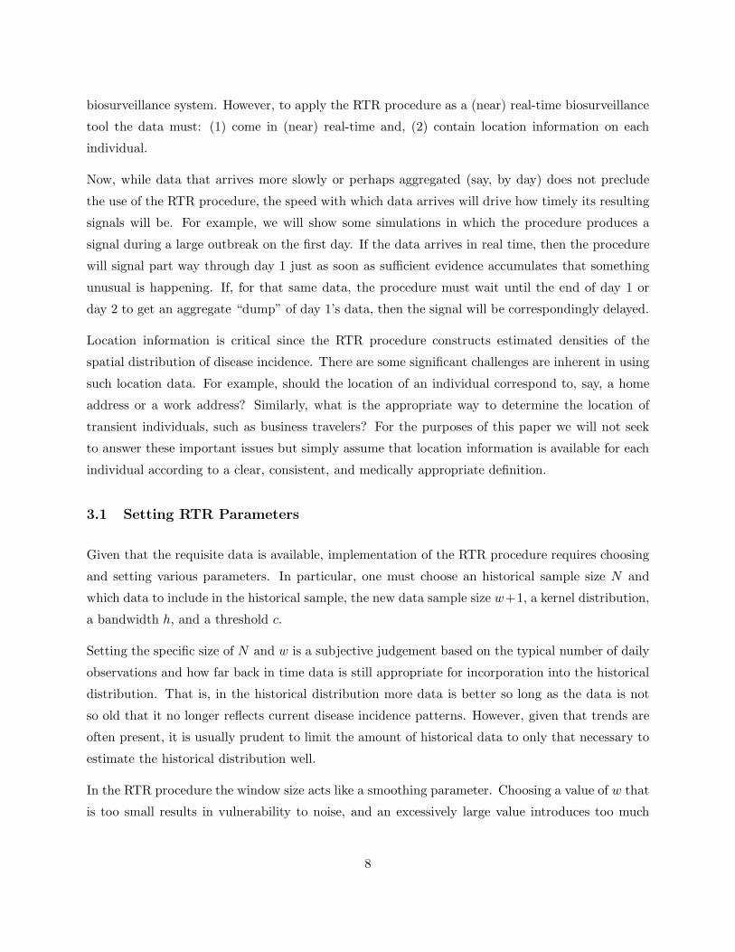
Individual realizations of the three scenarios are shown in Figures 1 through 3 for the first 11 days
of each outbreak. Day 0 is the day prior to the outbreak.
The first column in each figure shows the distribution of the expected number of cases where the
area under the surface for some subregion represents the expected number of cases in that subregion.
Of course, in real biosurveillance this distribution is unobserved. As just described, for all three
scenarios the background disease incidence follows a simple bivariate normal distribution with an
expected number of 30 cases per day. The outbreaks start on day 1 in each figure and show up as
an outbreak distribution overlaid on the background disease distribution. The progression of the
outbreak distribution can then be followed for the first 11 days.
The second column shows the observations that occurred on each day. On day 0 of each scenario
there are about 30 observations generated according to the background disease distribution. Start-
ing on day 1 outbreak observations are intermixed according to each scenario’s outbreak type and
expected number. On day d, the expected number of outbreak observations is d in Scenario #1,
d2 in Scenario #2, and 64 in Scenario #3.
Finally, the third column shows the contours of the difference between the kernel density estimate
for the N historical observations and the kernel density estimate of the w + 1 new observations
calculated as follows. To simplify the notation, assume n > w + 1 and so define the kernel density
11
D Contours D ContoursA Dist’n of Daily of KDE A Dist’n of Daily of KDEY Expected Nr. Observations Differences Y Expected Nr. Observations Differences
0-40
-200
20
40-40
-20
0
20
40
-40-20
0
20
40
-40 -30 -20 -10 10 20 30 40
-40
-30
-20
-10
10
20
30
40
-40 -20 0 20 40-40
-20
0
20
40
6-40
-200
20
40-40
-20
0
20
40
-40-20
0
20
40
-40 -30 -20 -10 10 20 30 40
-40
-30
-20
-10
10
20
30
40
-40 -20 0 20 40-40
-20
0
20
40
1-40
-200
20
40-40
-20
0
20
40
-40-20
0
20
40
-40 -30 -20 -10 10 20 30 40
-40
-30
-20
-10
10
20
30
40
-40 -20 0 20 40-40
-20
0
20
40
7-40
-200
20
40-40
-20
0
20
40
-40-20
0
20
40
-40 -30 -20 -10 10 20 30 40
-40
-30
-20
-10
10
20
30
40
-40 -20 0 20 40-40
-20
0
20
40
2-40
-200
20
40-40
-20
0
20
40
-40-20
0
20
40
-40 -30 -20 -10 10 20 30 40
-40
-30
-20
-10
10
20
30
40
-40 -20 0 20 40-40
-20
0
20
40
[8]-40
-200
20
40-40
-20
0
20
40
-40-20
0
20
40
-40 -30 -20 -10 10 20 30 40
-40
-30
-20
-10
10
20
30
40
-40 -20 0 20 40-40
-20
0
20
40
3-40
-200
20
40-40
-20
0
20
40
-40-20
0
20
40
-40 -30 -20 -10 10 20 30 40
-40
-30
-20
-10
10
20
30
40
-40 -20 0 20 40-40
-20
0
20
40
9-40
-200
20
40-40
-20
0
20
40
-40-20
0
20
40
-40 -30 -20 -10 10 20 30 40
-40
-30
-20
-10
10
20
30
40
-40 -20 0 20 40-40
-20
0
20
40
4-40
-200
20
40-40
-20
0
20
40
-40-20
0
20
40
-40 -30 -20 -10 10 20 30 40
-40
-30
-20
-10
10
20
30
40
-40 -20 0 20 40-40
-20
0
20
40
10-40
-200
20
40-40
-20
0
20
40
-40-20
0
20
40
-40 -30 -20 -10 10 20 30 40
-40
-30
-20
-10
10
20
30
40
-40 -20 0 20 40-40
-20
0
20
40
5-40
-200
20
40-40
-20
0
20
40
-40-20
0
20
40
-40 -30 -20 -10 10 20 30 40
-40
-30
-20
-10
10
20
30
40
-40 -20 0 20 40-40
-20
0
20
40
11-40
-200
20
40-40
-20
0
20
40
-40-20
0
20
40
-40 -30 -20 -10 10 20 30 40
-40
-30
-20
-10
10
20
30
40
-40 -20 0 20 40-40
-20
0
20
40
Figure 1: Scenario #1 begins with a background disease incidence distributed according to abivariate normal centered at {0, 0} with an average of 30 observations per day. On day 1 anoutbreak begins, centered at {20, 20} which grows linearly over time and spreads. On day d theexpected number of outbreak cases is d.
12
D Contours D ContoursA Dist’n of Daily of KDE A Dist’n of Daily of KDEY Expected Nr. Observations Differences Y Expected Nr. Observations Differences
0-40
-200
20
40-40
-20
0
20
40
-40-20
0
20
40
-40 -30 -20 -10 10 20 30 40
-40
-30
-20
-10
10
20
30
40
-40 -20 0 20 40-40
-20
0
20
40
6-40
-200
20
40-40
-20
0
20
40
-40-20
0
20
40
-40 -30 -20 -10 10 20 30 40
-40
-30
-20
-10
10
20
30
40
-40 -20 0 20 40-40
-20
0
20
40
1-40
-200
20
40-40
-20
0
20
40
-40-20
0
20
40
-40 -30 -20 -10 10 20 30 40
-40
-30
-20
-10
10
20
30
40
-40 -20 0 20 40-40
-20
0
20
40
7-40
-200
20
40-40
-20
0
20
40
-40-20
0
20
40
-40 -30 -20 -10 10 20 30 40
-40
-30
-20
-10
10
20
30
40
-40 -20 0 20 40-40
-20
0
20
40
2-40
-200
20
40-40
-20
0
20
40
-40-20
0
20
40
-40 -30 -20 -10 10 20 30 40
-40
-30
-20
-10
10
20
30
40
-40 -20 0 20 40-40
-20
0
20
40
8-40
-200
20
40-40
-20
0
20
40
-40-20
0
20
40
-40 -30 -20 -10 10 20 30 40
-40
-30
-20
-10
10
20
30
40
-40 -20 0 20 40-40
-20
0
20
40
3-40
-200
20
40-40
-20
0
20
40
-40-20
0
20
40
-40 -30 -20 -10 10 20 30 40
-40
-30
-20
-10
10
20
30
40
-40 -20 0 20 40-40
-20
0
20
40
9-40
-200
20
40-40
-20
0
20
40
-40-20
0
20
40
-40 -30 -20 -10 10 20 30 40
-40
-30
-20
-10
10
20
30
40
-40 -20 0 20 40-40
-20
0
20
40
[4]-40
-200
20
40-40
-20
0
20
40
-40-20
0
20
40
-40 -30 -20 -10 10 20 30 40
-40
-30
-20
-10
10
20
30
40
-40 -20 0 20 40-40
-20
0
20
40
10-40
-200
20
40-40
-20
0
20
40
-40-20
0
20
40
-40 -30 -20 -10 10 20 30 40
-40
-30
-20
-10
10
20
30
40
-40 -20 0 20 40-40
-20
0
20
40
5-40
-200
20
40-40
-20
0
20
40
-40-20
0
20
40
-40 -30 -20 -10 10 20 30 40
-40
-30
-20
-10
10
20
30
40
-40 -20 0 20 40-40
-20
0
20
40
11-40
-200
20
40-40
-20
0
20
40
-40-20
0
20
40
-40 -30 -20 -10 10 20 30 40
-40
-30
-20
-10
10
20
30
40
-40 -20 0 20 40-40
-20
0
20
40
Figure 2: Scenario #2 also begins with a background disease incidence distributed according toa bivariate normal centered at {0, 0} with an average of 30 observations per day. On day 1 anoutbreak begins, centered at {20, 20}, which grows quadratically over time and spreads faster thanthe outbreak in Scenario #1. On day d the expected number of outbreak cases is d2.
13
D Contours D ContoursA Dist’n of Daily of KDE A Dist’n of Daily of KDEY Expected Nr. Observations Differences Y Expected Nr. Observations Differences
0-40
-200
20
40-40
-20
0
20
40
-40-20
0
20
40
-40 -30 -20 -10 10 20 30 40
-40
-30
-20
-10
10
20
30
40
-40 -20 0 20 40-40
-20
0
20
40
6-40
-200
20
40-40
-20
0
20
40
-40-20
0
20
40
-40 -30 -20 -10 10 20 30 40
-40
-30
-20
-10
10
20
30
40
-40 -20 0 20 40-40
-20
0
20
40
[1]-40
-200
20
40-40
-20
0
20
40
-40-20
0
20
40
-40 -30 -20 -10 10 20 30 40
-40
-30
-20
-10
10
20
30
40
-40 -20 0 20 40-40
-20
0
20
40
7-40
-200
20
40-40
-20
0
20
40
-40-20
0
20
40
-40 -30 -20 -10 10 20 30 40
-40
-30
-20
-10
10
20
30
40
-40 -20 0 20 40-40
-20
0
20
40
2-40
-200
20
40-40
-20
0
20
40
-40-20
0
20
40
-40 -30 -20 -10 10 20 30 40
-40
-30
-20
-10
10
20
30
40
-40 -20 0 20 40-40
-20
0
20
40
8-40
-200
20
40-40
-20
0
20
40
-40-20
0
20
40
-40 -30 -20 -10 10 20 30 40
-40
-30
-20
-10
10
20
30
40
-40 -20 0 20 40-40
-20
0
20
40
3-40
-200
20
40-40
-20
0
20
40
-40-20
0
20
40
-40 -30 -20 -10 10 20 30 40
-40
-30
-20
-10
10
20
30
40
-40 -20 0 20 40-40
-20
0
20
40
9-40
-200
20
40-40
-20
0
20
40
-40-20
0
20
40
-40 -30 -20 -10 10 20 30 40
-40
-30
-20
-10
10
20
30
40
-40 -20 0 20 40-40
-20
0
20
40
4-40
-200
20
40-40
-20
0
20
40
-40-20
0
20
40
-40 -30 -20 -10 10 20 30 40
-40
-30
-20
-10
10
20
30
40
-40 -20 0 20 40-40
-20
0
20
40
10-40
-200
20
40-40
-20
0
20
40
-40-20
0
20
40
-40 -30 -20 -10 10 20 30 40
-40
-30
-20
-10
10
20
30
40
-40 -20 0 20 40-40
-20
0
20
40
5-40
-200
20
40-40
-20
0
20
40
-40-20
0
20
40
-40 -30 -20 -10 10 20 30 40
-40
-30
-20
-10
10
20
30
40
-40 -20 0 20 40-40
-20
0
20
40
11-40
-200
20
40-40
-20
0
20
40
-40-20
0
20
40
-40 -30 -20 -10 10 20 30 40
-40
-30
-20
-10
10
20
30
40
-40 -20 0 20 40-40
-20
0
20
40
Figure 3: Scenario #3 begins with a background disease incidence distributed according to abivariate normal centered at {0, 0} with an average of 30 observations per day. Starting on day 1,an outbreak sweeps across the region from left to right generating an extra 64 cases per day.
14
estimate for the historical data as
gn(x) =1
N
n−w−1∑
i=n−w−N−1
kh(x,Xi)
where the kernel function is a bivariate normal and the bandwidth is hi = σi
(1N
)1/6, i = 1, 2.
Similarly, define the kernel density estimate for the new data as
hn(x) =1
w + 1
n∑
i=n−w
kh(x,Xi)
where the kernel function is a bivariate normal and the bandwidth is hi = σi
(1
w+1
)1/6, i = 1, 2.
Then plot
∆n(x) = max(
δ, hn(x) − gn(x))
, (10)
where δ is a small positive number that helps eliminate excess noise from the plots. For Figures 1
through 3 we used δ = 0.00011.
A number of observations arise upon examination of Figures 1 through 3. First, early in Scenarios
#1 and #2 the scatterplots provide no visual indication that an outbreak is occurring. However,
the contours of the kernel density estimate (KDE) differences from Equation (10) correspond nicely
to the known outbreak areas. Furthermore, the sequence of the kernel density estimate differences
tracks well with the growth of the outbreaks.
That said, it would be erroneous to assume that the contours are sufficient for identifying the
outbreaks. This is because it is possible for contours to be visible even when an outbreak is not
occurring. To illustrate, see Figure 4 which shows the contour plots for days 0-5 in Scenario #1
from Figure 1 along with the complete surface plots. Here we see that the differences between the
density estimates is noisy and this noise can sometimes show up on the contour plots.
Thus, we supplement a visual inspection of the plots with an analysis of the data using the RTR
procedure to signal when a change has occurred. The day on which the RTR signalled when applied
to the actual data in each figure is indicated by the day number in brackets: in Figure 1, the RTR
signalled on observation 274 on day 8; in Figure 2 the RTR signalled on observation 173 on day
5; and in Figure 3 the RTR signalled on observation 14 on day 1. This latter result indicates the
utility of a procedure that operates sequentially on the individual observations. Were the data
aggregated by day, then a signal would not have been generated until day 2, in spite of the fact
that by then the outbreak in this case is obvious just by looking at the scatterplot. Instead, the
15
-40 -20 0 20 40-40
-20
0
20
40
-40-20
0
20
40-40
-20
0
20
40
-40-20
0
20
-40 -20 0 20 40-40
-20
0
20
40
-40-20
0
20
40-40
-20
0
20
40
-40-20
0
20
-40 -20 0 20 40-40
-20
0
20
40
-40-20
0
20
40-40
-20
0
20
40
-40-20
0
20
-40 -20 0 20 40-40
-20
0
20
40
-40-20
0
20
40-40
-20
0
20
40
-40-20
0
20
-40 -20 0 20 40-40
-20
0
20
40
-40-20
0
20
40-40
-20
0
20
40
-40-20
0
20
-40 -20 0 20 40-40
-20
0
20
40
-40-20
0
20
40-40
-20
0
20
40
-40-20
0
20
Figure 4: Contour plots and their associated surfaces for days 0-5 in Scenario #1 from Figure 1.
16
1 2 3 4 5 6 7 8Day
5
10
15
20
25
30
Percent
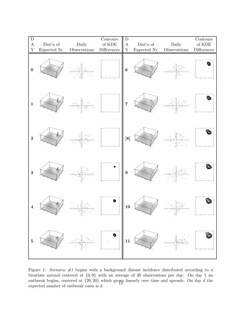
Figure 5: For Scenario #1, a plot of the percentage of times the RTR stopped on a particular dayof the outbreak.
RTR procedure signalled that something unusual seemed to be going on after only 14 observations
– roughly 15 percent of the observations that would occur on that day.
Of course, these are only one realization for each of the scenarios and, in fact, the results beg the
question as to how the RTR procedure would perform over many trials. As the next section shows,
the signal in only 14 observations in Figure 3 was a bit faster than how the RTR would perform
on average for Scenario #3 while the stopping times for the Figures 1 and 2 turn out to be longer
than the average for Scenarios #1 and #2.
3.3 Demonstrating the RTR’s Performance
To assess how the RTR procedure performed more generally, we ran it many times on each scenario
and recorded the day and the observation number when the RTR signaled. For example, Figure 5
shows that under Scenario #1 the RTR predominantly signalled on either the 5th or 6th day of the
outbreak. Remember that the Scenario #1 the outbreak increased linearly, so that by the end of
the fifth day 15 outbreak observations had been observed on average (in addition to an average of
150 non-outbreak observations). The average number of observations until the RTR signalled was
146, or roughly in the middle of the 5th day.
17
1 2 3 4Day
5
10
15
20
25
30
35
Percent
Figure 6: For Scenario #2, a plot of the percentage of times the RTR stopped on a particular dayof the outbreak.
In contrast, Figure 6 shows that under Scenario #2 the RTR predominantly signalled on the 3rd
or 4th day of the outbreak. This makes sense since under Scenario #2 the outbreak increased
quadratically and so should have been easier to detect than the Scenario #1 outbreak. In fact,
by the end of the third day on average 14 outbreak (and 90 non-outbreak) observations had been
observed compared to an average of 15 at the end of the 5th day in Scenario #1. Under Scenario
#2, the average number of observations until the RTR signalled was 80, or roughly in the middle
of the third day of an outbreak.
Now, under Scenario #3, the RTR always signalled on the first day. It did so because even just a
few observations far out on the periphery of the region would be unusual. Indeed, a simple visual
examination of the scatterplots in Figure 3 make it clear that something abnormal is occurring
(assuming one knows what the normal pattern looks like). In fact, it took only 23 observations on
average until a signal was produced. Given that each day would get, on average 94 observations
(64 outbreak and 30 non-outbreak), that means the RTR signalled less than one-third of the way
through the first day and after observing about 15 outbreak observations.
18
4 Conclusions
This paper has demonstrated the application of the Repeated Two-Sample Rank procedure to the
problem of biosurveillance and it has shown that methodology supports both goals of syndromic
surveillance systems: early event detection and situational awareness. Furthermore, because the
RTR procedure is designed to incorporate the information from each individual observation as it
sequentially arrives into such a system, the methodology can provide more timely signals than
those methods that aggregate data. Indeed, in the simulations we observed that an average of 14
or 15 outbreak observations was sufficient to cause a signal and the RTR was able to synthesize
the information from those observations whether they occurred in one day or across many days.
In addition, via the use of kernel density estimation, the RTR eliminates the issues faced by other
methods which must aggregate data within artificial spatial boundaries (e.g., zip codes). Finally,
theoretical results are available to assist the public health practitioner or biosurveillance system
designer in choosing the necessary algorithmic parameters such as the kernel bandwidth and the
threshold.
The RTR procedure does have some limitations. Most importantly, it is incapable of detecting
an increase in disease incidence if the increase is randomly distributed over the region according
the background disease incidence (non-outbreak) distribution. If this is of concern then the RTR
procedure will have to be augmented with an appropriate temporal method. However, we expect
that a disease outbreak or a bioterrorism event is very unlikely to manifest itself in such a fashion.
Rather, our sense is that a general increase in disease incidence is likely to be the result of seasonal
fluctuations or perhaps some phenomenon related, say, to an aging population. As such, in the
context of bioterrorism detection, the RTR’s insensitivity to this type of change can be seen as an
advantage since it does not have to be adjusted to account for naturally-occurring incidence rate
changes the way temporal methods often must be.
The RTR as described in this paper is designed to account for changes in the distribution of back-
ground disease. It does this by using a moving window of historical data, for which we arbitrarily
chose a window 45 days in length. The idea is that, in biosurveillance, we are monitoring for
abrupt departures from recent patterns. The length of this window should be a function both of
how quickly the background incidence distribution changes and the rate of the observed data. The
key consideration is that the historical data should be of sufficient number to estimate well the
non-outbreak distribution and such that the resulting distribution is as current as possible. While
Section 2 described the historical sample as a moving window, it need not be so. In particular,
19
in biosurveillance settings in which the background disease incidence does not change (or changes
very little) over time, it may be preferable to use a fixed historical sample (see Fricker, 1997).
If a moving window of historical data is to be used, there are some practical considerations that
must be addressed in the implementation of the methodology related to how to adjust the historical
data set once an outbreak is identified. Simply put, it is important to ensure that the historical
sample is not contaminated with outbreak data. Such contamination could make it more difficult
to detect future outbreaks. See Fricker, Knitt and Hu (2008) for a discussion of these issues in a
related syndromic surveillance context.
Many other variations of the RTR procedure are possible. In this paper, we used density height
calculated from a kernel density estimate as the univariate statistic. In work not shown here, we
have compared this formulation against variants using data depth and Euclidean distance to near-
est neighbor statistics and found kernel density estimation to be preferable based on performance
and calculation considerations. We have also compared the use of the Kolmogorov-Smirnov non-
parametric test to the chi-squared test. We found the two perform similarly, and our preference
for the Kolmogorov-Smirnov test is based on not having to specify “bins.” It is also possible to use
an adaptive kernel density estimate, which may be preferable when there are subregions in which
the background disease incident counts are very low, but we have not explored the performance of
such a method in our research.
We conclude by noting that biosurveillance is but one application for the RTR procedure. As
described herein, it can be applied to many different types of spatio-temporal change detection,
from other types of public health problems, to problems in demography and geography, as well
as national security problems such as changes in the employment patterns of improvised explosive
devices in Iraq. In addition, though not described here, the RTR procedure can also be used as a
purely temporal nonparametric multivariate statistical process control methodology.
Acknowledgments. R. Fricker’s research was supported in part by Office of Naval Research grant
N0001407WR20172 and in part by funding from the Naval Postgraduate School.
20
References
Ackelsberg, J., Balter, S., Bornschelgel, K., Carubis, E., Cherry, C., Das, D., Fine, A., Karpati, A., Layton,M., Mostashari, F., Nivin, B., Reddy, V., Weiss, D., Hutwagner, L., Seeman, G.M., McQuiston, J., Treadwell,T., and J. Rhodes (2002). Syndromic Surveillance for Bioterrorism Following the Attacks on the World TradeCenter - New York City, 2001, Morbidity and Mortality Weekly Report, 51 (Special Issue), Centers for DiseaseControl and Prevention, pp. 13–15.
Aldous, D. (1989). Probability Approximations via the Poisson Clumping Heuristic, Springer-Verlag, NewYork, New York.
Bowman, A.W., and A. Azzalini (2004). Applied Smoothing Techniques for Data Analysis: The Kernel
Bravata, D.M., McDonald, K.M., Smithe, W.M., Rydzak, C., Szeto, H., Buckeridge, D.L., Haberland, C., andD.K. Owens (2004). Systematic review: Surveillance Systems for Early Detection of Bioterrorism-RelatedDiseases, Annals of Internal Medicine, 140, 11, pp. 910–922.
Diggle, P.J., Rowlingsos, B., and T. Su (2004). Point Process Methodology for On-line Spatio-temporalDisease Surveillance, Johns Hopkins University, Department of Biostatistics Working Papers, paper 37.
Forsberg, L., Jeffery, C., Ozonoff, A., and M. Pagano (2006). A Spatiotemporal Analysis of SyndromicData for Biosurveillance, Statistical Methods in Counterterrorism: Game Theory, Modeling, Syndromic
Surveillance, and Biometric Authentication, A. Wilson, G. Wilson, and D.H. Olwell, eds., Springer, NewYork, NY, pp. 173–191.
Fricker, R.D., Jr. (2007). Syndromic Surveillance, Encyclopedia of Quantitative Risk Assessment (to appear).
Fricker, R.D., Jr., Knitt, M.C., and C.X. Hu (2007). Comparing Directionally Sensitive MCUSUM andMEWMA Procedures with Application to Biosurveillance, Quality Engineering (to appear).
Fricker, R.D., Jr., and H. Rolka (2006). Protecting Against Biological Terrorism: Statistical Issues inElectronic Biosurveillance, Chance, 91, pp. 4–13.
Fricker, R.D., Jr. (1997). Nonparametric Control Charts for Multivariate Data, Ph.D. Thesis, Yale Univer-sity.
Kleinman, K., Lazarus, R., and R. Platt (2004). A Generalized Mixed Model Approach for DetectingIncident Clusters of Disease in Small Areas, with an Application to Biological Terrorism, American Journal
of Epidemiology, 159, pp. 217–224.
Kulldorff, M. (2001). Prospective Time Periodic Geographical Disease Surveillance Using a Scan Statistic,Journal of the Royal Statistical Society, Series A (Statistics in Society), 164, pp. 61–72. Accessed online atwww.satscan.org/papers/k-jrssa2001.pdf on November 28, 2006.
Kulldorff, M. (1997). A Spatial Scan Statistic, Communications in Statistics, Theory and Methods, 26, pp.1481–1496. Accessed online at www.satscan.org/papers/k-cstm1997.pdf on November 28, 2006.
Lazarus, R., Kleinman, K., Dashevsky, I., Adams, C., Kludt, P., DeMaria, Jr., A., and R. Platt (2002). Use ofAutomated Ambulatory-Care Encounter Records for Detection of Acute Illness Clusters, Including PotentialBioterrorism Events, Emerging Infectious Diseases, 8, pp. 753–760. Accessed online at www.medscape.com/viewarticle/440756 print on November 28, 2006.
21
Lawson, A.B., and K. Kleinman (eds.) (2005). Spatial and Syndromic Surveillance for Public Health, JohnWiley & Sons.
Mandl, K.D., Overhage, J.M., Wagner, M.W., Lober, W.B., Sebastiani, P., Mostashari, F., Pavlin, J.A.,Gesteland, P.H., Treadwell, T., Koski, E., Hutwagner, L., Buckeridge, D.L., Aller, R.D., S. Grannis (2004).Implementing Syndromic Surveillance: A Practical Guide Informed by the Early Experience, The Journal of
the American Medical Informatics Association, 11, pp. 141–150. Accessed online at www.pubmedcentral.nih.gov/articlerender.fcgi?artid=353021 on November 28, 2006.
Montgomery, D.C. (2001). Introduction to Statistical Quality Control, 4th edition, John Wiley & Sons, NewYork.
Olson, K.L., Bonetti, M., Pagano, M., and K.D. Mandl (2005). Real Time Spatial Cluster Detection UsingInterpoint Distances Among Precise Patient Locations, BMC Medical Informatics and Decision Making, 5.Accessed online at www.biomedcentral.com/1472-6947/5/19 on December 4, 2006.
Randles, R.H. and Wolfe, D.A. (1979). Introduction to the Theory of Nonparametric Statistics, John Wiley& Sons, New York, New York.
Rogerson, P.A., and I. Yamada (2004). Monitoring Change in Spatial Patterns of Disease: ComparingUnivariate and Multivariate Cumulative Sum Approaches, Statistics in Medicine, 23, pp. 2195–2214.
Shmueli, G., and S.E. Fienberg (2006). Current and Potential Statistical Methods for Monitoring MultipleData Streams for Biosurveillance, Statistical Methods in Counterterrorism: Game Theory, Modeling, Syn-
dromic Surveillance, and Biometric Authentication, A. Wilson, G. Wilson, and D.H. Olwell, eds., Springer,New York, NY, pp. 109–140.
Shmueli, G. (2006). Statistical Challenges in Modern Biosurveillance, in submission to Technometrics, draftdated September 18, 2006.
Sonesson, C. (2007). A CUSUM Framework for Detection of Space-time Disease Clusters using Scan Statis-tics, Statistics in Medicine (in press).
Sosin, D. (2005). Evaluation Challenges for Syndromic Surveillance - Making Incremental Progress, Mor-
bidity and Mortality Weekly Report, 53 (Supplemental), Centers for Disease Control and Prevention, pp.125–129.
Sosin, D.M. (2003). Syndromic Surveillance: The Case for Skillful Investment View, Biosecurity and Bioter-
rorism: Biodefense Strategy, Practice, and Science, 1, 247–253. Accessed online at www.medscape.com/viewarticle/466780 on November 22, 2006.
Waller, L.A., and C.A. Gotway (2004). Applied Spatial Statistics for Public Health Data, John Wiley &Sons.
Woodall, W.H., Marshall, J.B., Joner, M.D., Jr., Fraker, S.E., and A.G. Abdel-Salam (2007). On the Use ofScan Methods in Prospective Public Health Surveillance, to be submitted to Journal of the Royal Statistical
Society, Series A (Statistics in Society). Draft dated March 8, 2007.
Woodall, W.H. (2006). The Use of Control Charts in Health-Care and Public-Health Surveillance, Journal