Page 1
HAL Id: tel-01732145https://tel.archives-ouvertes.fr/tel-01732145
Submitted on 14 Mar 2018
HAL is a multi-disciplinary open accessarchive for the deposit and dissemination of sci-entific research documents, whether they are pub-lished or not. The documents may come fromteaching and research institutions in France orabroad, or from public or private research centers.
L’archive ouverte pluridisciplinaire HAL, estdestinée au dépôt et à la diffusion de documentsscientifiques de niveau recherche, publiés ou non,émanant des établissements d’enseignement et derecherche français ou étrangers, des laboratoirespublics ou privés.
A speaker recognition system based on vocal cords’vibrationsDany Ishak
To cite this version:Dany Ishak. A speaker recognition system based on vocal cords’ vibrations. Micro and nanotechnolo-gies/Microelectronics. Université de Valenciennes et du Hainaut-Cambresis; Université de Balamand(Tripoli, Liban), 2017. English. �NNT : 2017VALE0043�. �tel-01732145�
Page 2
Doctoral thesis
To obtain the degree of Doctor of the University of
VALENCIENNES AND HAINAUTCAMBRESIS
Specialty: ELECTRONICS
Defended by Dany ISHAK
On 19/12/2017, at the IEMN-DOAE Amphitheater, University of Valenciennes
Doctoral school:
Sciences Pour l’Ingénieur (SPI)
Research teams, Laboratories:
Institut d’Electronique, de Micro-Electronique et de Nanotechnologie/Département d’Opto-Acousto-Electronique (IEMN/DOAE)
A Speaker Recognition System based on Vocal Cords’ Vibrations
JURY
President
- Restoin, Christine. Professor, University of Limoges.
Reviewers
- Grisel, Richard. Professor at INSA Rouen. - Rihana, Sandy. Associate Professor, Holy Spirit University of Kaslik.
Examiner
- Ayoubi, Rafic. Associate Professor, University of Balamand. Co-director: Nassar, Georges. Maître de conférences-HDR, Université de Valenciennes. Co-director: Abche, Antoine. Professor, University of Balamand. Co-supervisor: Callens, Dorothée. Maître de conférences, Université de Valenciennes. Co-supervisor: Karam, Elie. Professor, University of Balamand.
Page 3
Thèse de doctorat
Pour obtenir le grade de Docteur de l’Université de
VALENCIENNES ET DU HAINAUTCAMBRESIS
Spécialité : ELECTRONIQUE
Présentée et soutenue par Dany ISHAK
Le 19/12/2017, à l’Amphithéâtre IEMN-DOAE, Université de Valenciennes
Ecole doctorale :
Sciences Pour l’Ingénieur (SPI)
Equipes de recherche, Laboratoires :
Institut d’Electronique, de Micro-Electronique et de Nanotechnologie/Département d’Opto-Acousto-Electronique (IEMN/DOAE)
La conception d’un système ultrasonore passif couche mince pour l’évaluation de l’état vibratoire des cordes vocales
JURY
Président du jury
- Restoin, Christine. Professeur à l’Université de Limoges.
Rapporteurs
- Grisel, Richard. Professeur à l’INSA de Rouen. - Rihana, Sandy. Associate Professor, Holy Spirit University of Kaslik.
Examinateur
- Ayoubi, Rafic. Associate Professor, Université de Balamand. Co-directeur de thèse : Nassar, Georges. Maître de conférences-HDR, Université de Valenciennes. Co-directeur de thèse : Abche, Antoine. Professeur, Université de Balamand. Co-encadrant : Callens, Dorothée. Maître de conférences, Université de Valenciennes. Co-encadrant : Karam, Elie. Professeur, Université de Balamand.
Page 4
Shoot for the moon.
Even if you miss, you’ll land among the stars.
Norman Vincent Peale, Les Brown.
Page 5
iv
ACKNOWLEDGEMENTS
The work presented in this PhD thesis has been performed under a collaboration between
IEMN - D. OAE (Institut d’Electronique, de Microélectronique et de Nanotechnologie,
Département Opto-Acousto-Electronique) in UVHC (Université de Valenciennes et du Hainaut
Cambrésis) - France and department of Computer and Electrical Engineering in University of
Balamand (UOB) - Lebanon.
This project could not have been accomplished without the contribution and the
encouragement of various people who had offered a great support. First, I would like to show my
greatest appreciation to my supervisors Dr. Antoine Abche (UOB) and Dr. Georges Nassar
(UVHC) for their persistent help, valuable guidance and advice. Their willingness to motivate
me contributed enormously to the project. It was their confidence in answering all the questions
and their support and constructive suggestions that have led to the accomplishment of this
project.
Second, I will take this opportunity to express my gratitude to my co-supervisors Dr. Elie
Karam (UOB) and Dr. Dorothée Callens (UVHC). The success of this project depends on their
encouragement and guidelines.
Third, I would like to thank warmly the members of the jury for agreeing and devoting
their time to judge my work.
Fourth, I would like to thank the National Instrument support team, and especially
Engineer Ralph Saab (District manager), for their help and their continuous support with the
technical aspects of the measurements.
I also want to thank my colleagues from both universities who provided me with a
continuous support and encouragement. In particular, I want to express my deep appreciation to
my best friends Daher Diab, Marie Semaan, Olga Yaacoub, Rania Minkara, Sandrine Matta and
Yasmine Jabaly for the fruitful discussions that we used to have and for creating a very pleasant
atmosphere at work.
Finally, there is no doubt that this project would have never come into life without the love
and the continuous support of my family. Their constant understanding, guidance and
encouragement have crowned all my efforts with success.
Page 6
v
ABSTRACT
In this work, a speaker recognition approach using a contact microphone is developed and
presented. The contact passive element is constructed from a piezoelectric material. In this
context, the position of the piezoelectric transducer on the individual’s neck may greatly affect
the quality of the collected signal and consequently the information extracted from it. Thus, the
multilayered medium in which the sound propagates before being detected by the transducer is
modeled. The best location on the individual’ neck to place a particular transducer element is
determined by implementing Monte Carlo simulation techniques and consequently, the
simulation results are verified using real experiments.
The recognition is based on the signal generated from the vocal cords’ vibrations when an
individual is speaking and not on the vocal signal at the output of the lips that is influenced by
the resonances in the vocal tract. Therefore, due to the varying nature of the collected signal, the
analysis was performed by applying the Short Term Fourier Transform technique to decompose
the signal into its frequency components. These frequencies represent the vocal folds’ vibrations
(50-1000 Hz). The features in terms of frequencies’ interval are extracted from the resulting
spectrogram. Then, a 1-D vector is formed for identification purposes. The identification of the
speaker is performed using two evaluation criteria, namely, the correlation similarity measure
and the Principal Component Analysis (PCA) in conjunction with the Euclidean distance. The
results show that a high percentage of recognition is achieved and the performance is much
better than many existing techniques in the literature.
Keywords: Biometric Identification, collar, contact microphone, correlation, diagnostic,
laryngophone, non acoustic sensor, piezoelectric transducer, PCA, physiological microphone (P-
mic), recursive stiffness matrix, speaker identification, speaker recognition, STFT, time-
frequency analysis, throat microphone.
Page 7
vi
RÉSUMÉ
Dans ce travail, une approche de reconnaissance de l’orateur en utilisant un microphone de
contact est développée et présentée. L'élément passif de contact est construit à partir d'un
matériau piézoélectrique. La position du transducteur piézoélectrique sur le cou de l'individu
peut affecter grandement la qualité du signal recueilli et par conséquent les informations qui en
sont extraites. Ainsi, le milieu multicouche dans lequel les vibrations des cordes vocales se
propagent avant d'être détectées par le transducteur est modélisé. Le meilleur emplacement sur le
cou de l’individu pour attacher un élément transducteur particulier est déterminé en mettant en
œuvre des techniques de simulation Monte Carlo et, par conséquent, les résultats de la simulation
sont vérifiés en utilisant des expériences réelles.
La reconnaissance est basée sur le signal généré par les vibrations des cordes vocales
lorsqu'un individu parle et non sur le signal vocal à la sortie des lèvres qui est influencé par les
résonances dans le conduit vocal. Par conséquent, en raison de la nature variable du signal
recueilli, l'analyse a été effectuée en appliquant la technique de transformation de Fourier à court
terme pour décomposer le signal en ses composantes de fréquence. Ces fréquences représentent
les vibrations des cordes vocales (50-1000 Hz). Les caractéristiques en termes d'intervalle de
fréquences sont extraites du spectrogramme résultant. Ensuite, un vecteur 1-D est formé à des
fins d'identification. L'identification de l’orateur est effectuée en utilisant deux critères
d'évaluation qui sont la mesure de la similarité de corrélation et l'analyse en composantes
principales (ACP) en conjonction avec la distance euclidienne. Les résultats montrent qu'un
pourcentage élevé de reconnaissance est atteint et que la performance est bien meilleure que de
nombreuses techniques existantes dans la littérature.
Mots clés: Analyse temps-fréquentielle, capteur non acoustique, corrélation, diagnostique,
identification biométrique, matrice de rigidité récursive, microphone de contact, microphone de
la gorge, laryngophone, reconnaissance de l’orateur, transducteur piézoélectrique, transformée de
Fourier de courte durée (STFT).
Page 8
vii
TABLE OF CONTENTS
ACKNOWLEDGEMENTS iv
ABSTRACT v
RÉSUMÉ vi
INTRODUCTION 1
Objective 2
Outline 3
CHAPTER 1: STATE OF ART 5
1.1 Introduction 5
1.2 Fundamentals of Voice Production 5
1.2.1 Breathing 5
1.2.2 Phonation 6
1.2.3 Resonance 8
1.3 Other Physical Factors 8
1.4 Vocal Signal Measurement Equipments 9
1.4.1 Electroglottograph 10
1.4.2 Tuned Electromagnetic Resonator Collar 12
1.4.3 Throat Microphone 13
1.4.4 Glottal Electromagnetic Micro-Power Sensor 14
1.4.5 Transnasal Flexible Endoscopy 15
1.4.5 Rigid Endoscopy 16
1.4.6 Stroboscopy 17
1.4.7 High Speed Video Endoscopy 18
1.5 Throat Microphone 19
1.5.1 Diagnostic 19
1.5.2 Speaker/Speech Recognition 20
1.6 Conclusion 24
Page 9
viii
CHAPTER 2: DEVELOPED APPROACH 25
2.1 Introduction 25
2.2 Developed Speaker Identification Approach 26
2.2.1 Signal Acquisition 31
2.2.1.1 Introduction 31
2.2.1.2 History 32
2.2.1.3 Domain of Application 33
2.2.1.4 Material’s characterization 34
2.2.1.5 Methodology 38
2.2.2 Short Time Fourier Transform 39
2.2.3 Normalization and Noise Removal 41
2.2.4 Features’ extraction 41
2.2.5 Database 42
2.2.6 Correlation 42
2.2.7 Principal Component Analysis (PCA) 43
2.3 Conclusion 45
CHAPTER 3: MODEL OF THE LAYERS OF THE HUMAN NECK 47
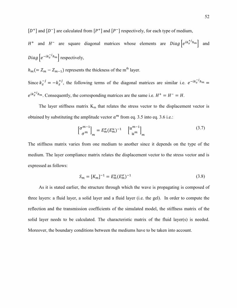
3.1 Introduction 47
3.2 System Model 48
3.2.1 Fluid Layer 53
3.2.2 Solid Layer 54
3.2.3 Fluid-Solid Interface 58
3.2.4 Reflection and Transmission Coefficients 58
3.2.5 Results 60
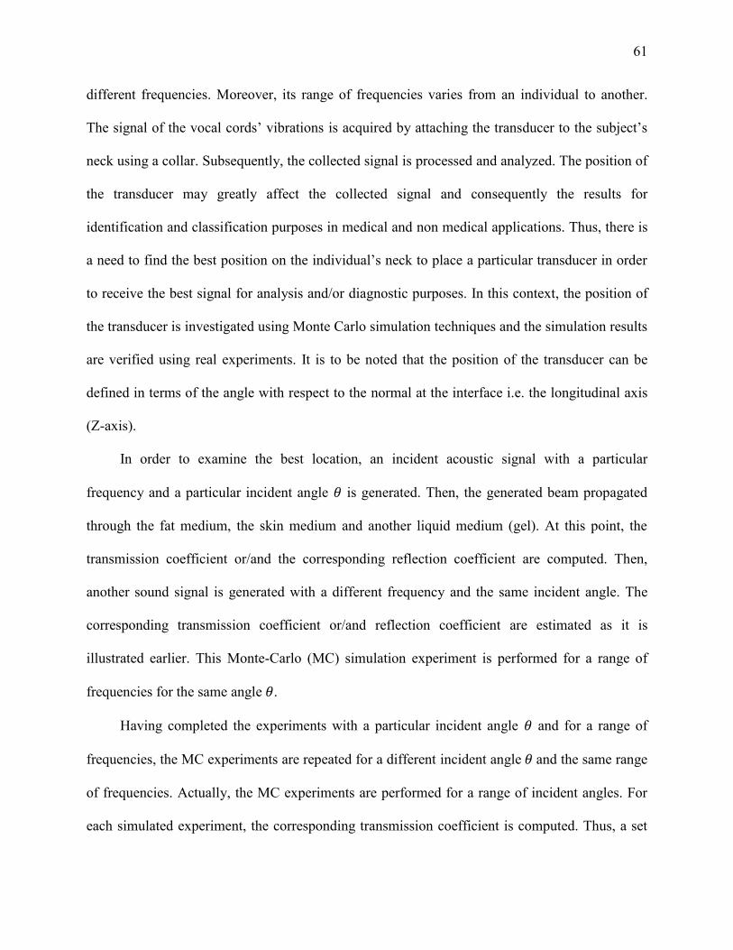
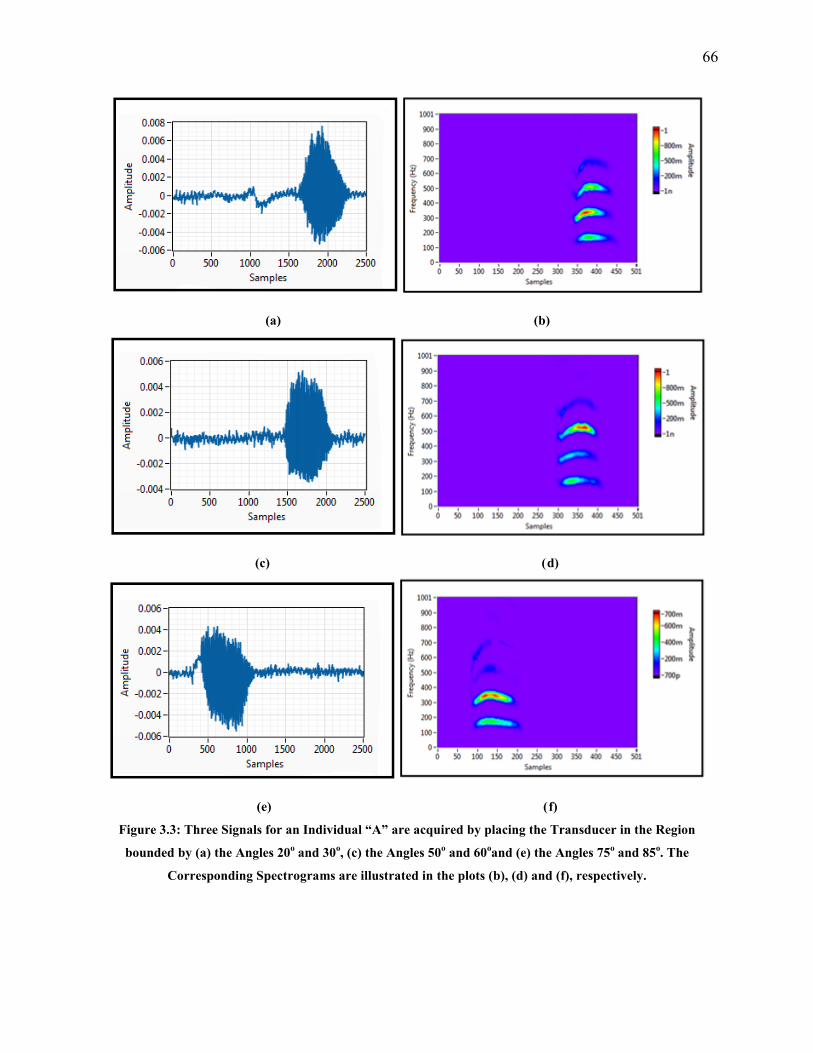
3.3 Experimental Evaluation 64
3.4 Conclusion 68
CHAPTER 4: RESULTS AND PERFORMANCE EVALUATION 70
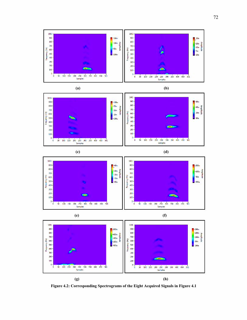
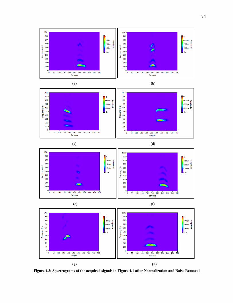
4.1 Introduction 70
4.2 Method 70
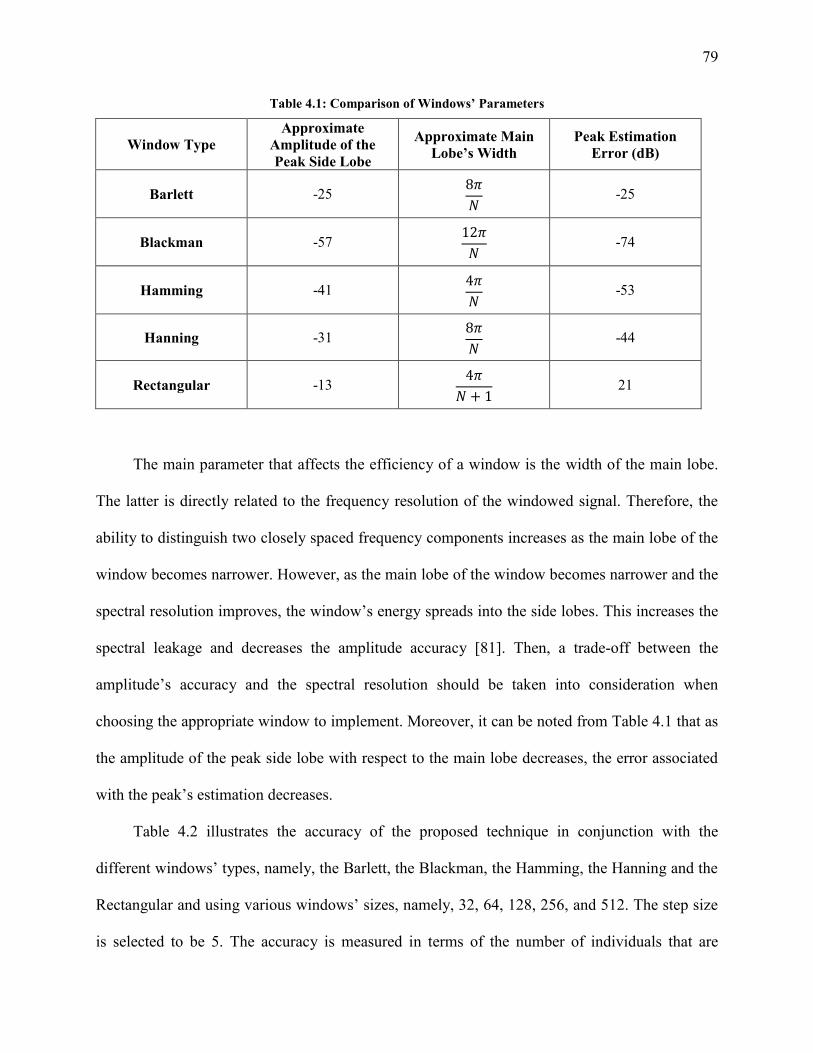
4.3 Effect of the Window 77
Page 10
ix
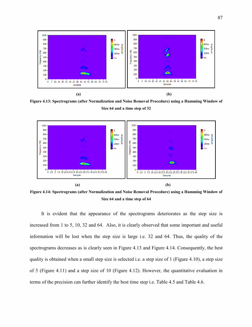
4.4 Effect of the Time Step 84
4.5 Evaluation with Other techniques 88
4.5.1 Wigner-Ville Distribution 88
4.5.2 Choi-Williams Distribution 89
4.5.3 Results and Discussion 90
4.5.4 Quantitative Evaluation 95
4.6 Conclusion 96
CONCLUSION 98
Recommendations and Future Prospects 99
LIST OF REFERENCES 101
Page 11
1
INTRODUCTION
Human beings need to communicate with each other. The human process of
communication has passed through many phases until the creation of the alphabet and the
beginning of the speaking languages known nowadays. For each language, the different sounds
emitted by the pronunciation of each letter enable the distinction and the detection of words and
consequently, the corresponding phrases [1].
From physical perspective, the human voice is generated by the coordination of three main
processes: the breathing, the phonation and the resonance [2]. The breathing of air out of the
lungs generates the necessary power supply for the voice. This airflow from the lungs causes the
vocal cords (or vocal folds) in the larynx to vibrate. The latter vibrations produce the
fundamental sound of the voice. This process is called the ‘Phonation’. Since the sound
generated by the vocal folds is too weak to be heard, it is modified into the known human voice’s
sound as it propagates from the larynx through the throat, the mouth and the nose. This process is
referred to as the resonance. The normal voice depends on how well the three fundamental
components (breathing, phonation and resonance) are synchronized.
The vocal cords’ vibrations in the larynx constitute the main source of the human sound
[2]. The measurement of these vibrations and the analysis of their respective frequencies have
been at the core of the researchers’ interest for many years and for various reasons. The latter
concept is implemented in various applications such as the speech signal de-noising, the speech
recognition, the speaker recognition and diagnostics.
The diagnosis of voice’s disorders was one of the main objectives of many acoustic and
non acoustic detection tools of the vocal cords’ vibrations. Diseases related to the vibrator device
(i.e. mainly the larynx and the vocal cords) are among the most common voice disorders. The
Page 12
2
acute laryngitis (inflammation of the vocal cords) is one of the most known diseases. It may in
particular cause what is commonly called the "loss of voice". It could happen to a teacher or a
professional singer and may lead to the total loss of the voice. This disorder usually lasts few
days and disappears completely. Other more serious pathologies can cause greater damage i.e.
some forms of laryngeal cancer. These forms of cancer are frequently directly related to smoking
(chronic) and are often associated with the excessive consumption of alcohol. These diseases
influence the voice’s vibrator device and subsequently, the frequencies of the vocal folds’
vibrations [1].
The frequencies of the vocal cords’ vibrations can also be analyzed to differentiate between
persons and to create a voice stamp that is specific to each individual. The speaker recognition,
an important biometric recognition mean, has been studied by researchers for many years.
Numerous network models and signal processing techniques have been developed and have been
tested for recognition and identification purposes [3]. The majority of the existing speaker
identification techniques is based on the individuals’ voices acquired usually using a
microphone. The approach that is presented in this thesis depends on the frequencies of the vocal
cords’ vibrations to identify the individuals and not the actual voices.
Objective
During the phase of phonation, the vocal folds vibrate with frequencies ranging from 50 Hz
to 1000 Hz. Such oscillations can be detected using technical devices only since the temporal
resolution of the human visual perception is limited to frequencies of about 20 Hz [4]. In this
context, the goal of this work is to build a non invasive tool that is able to detect the signal of
theses vibrations and consequently, to perform further processing on the collected signal in order
Page 13
3
to extract some useful information. This tool consists of a piezoelectric transducer element that is
built and attached to a collar. The latter collar is wrapped around the neck of the person. The
transducer’s piezoelectric material generates a charge when a pressure is applied and it vibrates
when a voltage is applied across the element. It basically transforms a mechanical energy into an
electrical energy and vice versa. When a mechanical vibration is applied, a current signal of
proportional intensity and of the same frequency will be generated.
In this work, a full theoretical study of the concept is developed and is presented. Then, a
set of measurements and experiments were conducted with the designed prototype device. The
developed device can be categorized as a contact microphone (throat microphone or
physiological microphone). It has shown a high level of efficiency and accuracy in a vital field
i.e. the speaker identification.
Outline
The human vocal system is explained in detail in Chapter 1. Then, a review of related
studies about the measurement of vocal folds’ vibrations using non acoustic sensors is presented.
At the end, numerous applications of the throat microphone in the speaker recognition area are
discussed.
The developed approach and the methodology of the proposed technique are presented and are
explained in Chapter 2.
In Chapter 3, the propagation of the sound through the multilayered medium from the vocal folds
to the surface of the neck is investigated and studied.
Page 14
4
Chapter 4 presents the results of the new developed speaker identification system which has
achieved a high degree of accuracy. The corresponding results are analyzed and are compared
with the results of other time-frequency techniques implemented in this work.
Finally, the conclusion section presents a summary of the presented work and its main
achievements as well as the prospects of future research in this area.
Page 15
5
CHAPTER 1
STATE OF ART
1.1 Introduction
‘You are how you sound’! That is, the voice’s tone tells the listeners a lot about the
character, emotions, feelings; as well as the actual thoughts of the speaker. Also, it can reveal a
great deal about his/her educational knowledge, social background, health and intellectual
awareness. Besides, the way he/she speaks has also the influence to make the listeners trust
him/her or to be viewed doubtfully. Unless there is a major physical disability in the voice
apparatus, each person is able to produce the type of voice that can serve his/her daily
communication needs [2].
1.2 Fundamentals of Voice Production
As stated earlier, the production of human voice passes through three main phenomena
which are the breathing, the phonation and the resonance. Each phenomenon will be discussed
below in details [2].
1.2.1 Breathing
The intent to produce a voice, as any other physical activity, starts from the brain. The
latter send impulses to the responsible components of the body. The body’s first response to
these signals is “breathing”. The air will enter into the lungs to power the voice. The breath is
ingested through the mouth and the nose, passes down the trachea (or windpipe) and is sniffed
into the lungs. The ribcage needs to inflate in order to let the air be inhaled into the lungs. Also,
the dome-like diaphragm which forms the base of the chest needs to extend downwards. After
Page 16
6
breathing successfully, most of the extension in the area of the lower ribs can be felt by the
individual. Having the lungs reached their maximum capacity from the air being inhaled, their
elastic tissues rebound and the air is exhaled or breathed out. The exhaled air comes up through
the trachea and then through the larynx where it confronts the closing vocal folds.
1.2.2 Phonation
During the breathing phase (without speaking), the vocal folds in the larynx are open
allowing the air to pass through the lungs easily. However, when the individual wants to speak,
the impulses sent from the brain directs the muscles of the larynx to close the vocal folds. When
the air returning up from the lungs confronts the closed vocal folds, the pressure and the flow of
the air overcome the resistance of the vocal folds which will be in a rapid vibration mode. These
rapid vibrations create the sound waves which propagate in the air and are the basic tones of the
person’s voice. Therefore, the vocal cords constitute the main source of the human voice.
The larynx is located on the top of the trachea. Its two vocal folds are approximately 20
mm in length. They are extended from the front of the neck to the back of the larynx. They have
a complex structure that is made up of four main layers. The outer layer is the mucous membrane
(or epithelium). An elastic layer filled with liquid is located below the outer layer. This layer is
known as the Reinke’s space. The mucous membrane and the Reinke’s space constitute both
what is known as the vocal cords’ ‘cover’. This cover must stay wet and flexible so that it can
move freely in a wave-like motion (the ‘mucosal wave’) over the profounder layers of the cords.
If it becomes dry or hard, the voice will become gruff and the person may experience throat
ache.
Page 17
7
Under the vocal folds’ cover, the vocal ligament is located. The latter is made up of
expandable tissues which enable the vocal cords to change shape easily when the deepest and the
least flexible layer, the muscle, changes its shape. The tone of the basic voice varies in diverse
ways and is depending on the vocal cords and other components of the voice mechanism. The
main aspects of the voice that can vary are: the pitch, the loudness and the quality.
1- Pitch: The pitch refers to the voice’s volume. It is determined primarily by the speed of
the vocal folds’ vibrations, the thickness of their edges and their lengths. When the rate
of the vocal cords’ vibrations goes faster, the voice becomes higher. The pitch will also
be higher as the vocal cords’ edges become more extended and thinner. On the other
hand, if the edges become thicker and shorter and the vocal cords vibrate at a slower
rate, the pitch will be lower. The variations of the pitch during the speech can indicate
the sense and the feeling and is referred to as the intonation.
2- Loudness: The loudness points to how sharp or quiet a voice is. The quantity of air
weight from the lungs and the muscle’s strains in the vocal folds are the two main
factors that control the loudness. The greater the air pressure is and the tenser the vocal
folds are the louder is the sound. A change in the loudness during a speech can also
show feelings and emotions and is referred to as stress. For example, the loudness of
the voice is increased sometimes when a particular word is spoken in order to show its
importance and to make the audience pay a particular attention.
3- Quality: The quality refers to the voice’s clearness. It is influenced by many factors.
The main factors are: the amount of relaxation of the larynx muscles, the degree of
humidity of the vocal cords’ cover, the amount of softness of the vocal folds’ vibrations
and the ability of the vocal cords to close properly during the phonation phase. The
Page 18
8
voice will sound gruff, tired and/or breathy if the muscles of the larynx are extremely
tough, the cover is dry, the folds move irregularly, and/or they cannot close properly.
1.2.3 Resonance
The vocal folds in the larynx produce sound waves known as the basic tone. The latter is
too weak to be recognized as a ‘voice’. Thus, it is amplified as it passes through the throat, the
mouth and the nose. The size, the shape and the muscle’s strain of these organs will define the
ultimate sound of the voice that is heard. Since the structures of the throat, the mouth and the
nose are different for each human being; the tone of the basic voice is different for each
individual. Therefore, each person has a clear unique timbre of voice. It is similar to what is
observed in musical instruments. That is, the size and the shape of a musical device, such as
trumpet, characterize the basic unique tone of the instrument. As the resonance process in a
trumpet makes it possible to control its sound throughout a concert hall, the resonance in the
human voice enables the control of its power and its projection.
1.3 Other Physical Factors
Besides the fundamental building blocks of the voice (breathing, phonation and resonance),
the efficiency of the voice is also influenced by two other main factors: the body position and the
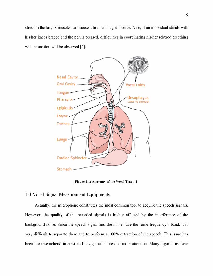
relaxation of the muscles of the body and the larynx. Figure 1.1 shows the anatomy of the organs
responsible to produce a voice i.e. anatomy of the vocal tract [2].
The body components that are responsible of the voice’s production are connected to other
components of the body’s muscular and skeletal system. Therefore, how the body is aligned and
the amount of the muscle’s strain or relaxation will affect the voice. For example, the overloaded
Page 19
9
stress in the larynx muscles can cause a tired and a gruff voice. Also, if an individual stands with
his/her knees braced and the pelvis pressed, difficulties in coordinating his/her relaxed breathing
with phonation will be observed [2].
Figure 1.1: Anatomy of the Vocal Tract [2]
1.4 Vocal Signal Measurement Equipments
Actually, the microphone constitutes the most common tool to acquire the speech signals.
However, the quality of the recorded signals is highly affected by the interference of the
background noise. Since the speech signal and the noise have the same frequency’s band, it is
very difficult to separate them and to perform a 100% extraction of the speech. This issue has
been the researchers’ interest and has gained more and more attention. Many algorithms have
Page 20
10
been developed in order to eliminate or to reduce to a large extent the embedded noise and the
majority have yielded good results. Besides, the research has been conducted to develop non
acoustic means to acquire the speech. Any sensor which is able to collect the speech before it
leaves the speaker’s lip/oral cavity is immune to the ambient environment noise [5, 6].
Non-acoustic measurement devices are usually robust and resistant to noise interference. In
the past two decades, experiments using non-acoustic sensors have revealed that it is feasible to
measure the glottal excitation and the articulator movements of the vocal cords in real-time as an
acoustic speech signal is generated. The non-acoustic sensors can be classified into two
categories: the physical instruments and the microwave devices. The physical instruments
include mainly the ElectroGlottoGraph (EGG), the Tuned Electromagnetic Resonator Collar
(TERC) sensor and the throat microphone. Among the microwave devices, the General
Electromagnetic Micro-Power Sensor (GEMS) has played an important role in this area. It was
used to measure the vocal folds’ vibrations during a speech. In addition, equipments such as the
transnasal flexible endoscopy, the rigid endoscopy, the stroboscopy and the high speed video
endoscopy have been designed to detect and to visualize the motion of the vocal folds [5-8].
1.4.1 ElectroGlottoGraph
The EGG (ElectroGlottoGraph) is a device that measures the Vocal Folds’ Contact Area
(VFCA) [9]. That is, it measures the variations in the electrical resistance between two electrodes
attached to the individual’s neck on each side of the thyroid cartilage (Figure 1.2). An electrical
signal in the MHz range is sent through the neck of the subject. The VFCA is determined by
observing the variations of the electrical impedance between the two electrodes when the vocal
cords are in a vibration mode (individual speaking). The EGG provides a physiological measure
Page 21
11
of the fundamental frequency (Fo) of the vocal cords’ vibrations at the laryngeal source’s level.
Compared to the acoustic signal, the EGG signal is much easier to analyze and to process [9-11].
Figure 1.2: Principle of the Electroglottograph [11]
The EGG has been implemented in many domains such as the speech recognition, the
speaker authentication and medical applications. However, since the EGG provides a measure of
the vocal cords’ contact, the sensor does not necessarily enable the observation of interesting
phenomena during the open phase of the glottis. It can be noted here that the EGG is not an exact
indicator of VFCA [9-11]. For example, during the transition to the open phase of the glottis, the
mucus can “short out” the machine. That is, the glottis is closed when it is actually not the case
i.e. the mucus bridging effect [12].
Page 22
12
1.4.2 Tuned Electromagnetic Resonator Collar
The Tuned Electromagnetic Resonator Collar (TERC) sensor is a non acoustic speech
sensor that is designed, as other non acoustic sensors, to measure the glottal activity during a
voiced speech [13]. However, the TERC has resolved many shortcomings of the existing
technology. First, the TERC sensor does not necessitate a direct skin contact. Second, it does not
require a critical positioning or alignment and is potent to the complex reflective environment of
the neck. Finally, unlike the ECG, the TERC sensor does not send any voltage or current through
the speaker.
The objective of the TERC sensor is to measure the variations of the relative permittivity
of the larynx as an alternative approach to measure the movement of the glottis. A common way
to determine the relative permittivity of a specific material is to create an electric field through
the material by building a capacitor (or an array of capacitors) and computing the resulting
capacitance. Figure 1.3 illustrates the concept of how a TERC speech sensor can be applied [13].
Figure 1.3: TERC Speech Sensor Basic Concept [13]
One or several capacitors are built around the neck’s tissues by attaching two or several
conductive plates on a collar that is wrapped around the speaker’s neck. There is no need for the
Page 23
13
collar to be in contact with the neck. However, it is suggested by the authors [13] to be worn as
shown in Figure 1.3 for convenience. Moreover, there is an insulation between the exposed
conductive plates and the speaker’s neck in order to prevent the skin’s contact and an unwanted
electrical conduction.
1.4.3 Throat Microphone
The Throat Microphone (TM), known also as the Physiological Microphone (PMIC), is a
non-acoustic sensor that captures the speech via the skin’s vibrations. The sensor is placed in
contact with the throat’s skin and close to the larynx. It detects the signals of the anatomical
vibrations that are generated during the speech along with the “buzz” tone of the larynx. Unlike
the standard microphone that gleans the variations of the air pressure and hence the background
noise; the throat microphone is more robust against the interference of the surrounding noise due
to its contact with the skin [6, 15]. People in different work environments could benefit from the
throat microphone to ensure a reliable voice communication. Fire fighters, law enforcement
officers and aircraft pilots are some relevant examples. In such environments, the noise
robustness of the throat microphone exceeds that of the normal microphone [6].
However, even though the throat’s microphone has a robust design against the background
noise, it is vulnerable to other noise interference and signal corruption such as the body
movement near the contact surface. Moreover, the improper placement of the sensor will lead to
the collection of a poor and corrupted signal. Therefore, there is a need to overcome these
shortcomings in order to have good results that can be properly analyzed [6].
Page 24
14
1.4.4 Glottal Electromagnetic Micro-Power Sensor
The GEMS (Glottal Electromagnetic Micro-power Sensor) is a non acoustic sensor that
measures the opening and the closing of the glottis and the vocal cords’ movements based upon
transmitting ElectroMagnetic (EM) waves into the glottal region. In other words, it measures the
tissues’ movements in the human’s vocal tract during the phonation (Figure 1.4), including the
vocal folds’ vibrations [5, 7, 9].
The old measurements with GEMS consist of strapping an antenna on the throat at the
laryngeal notch or at other facial locations. This set up can make the subjects discomfort and
sometimes may cause a skin irritation [5]. Subsequently, the radar technology has attracted a
great interest in different domains, such as medical monitoring, speech and speaker recognition.
Figure 1.4: Basic Concept of the Radar to detect the Signal of the Vocal Folds’ Vibrations [5]
Several studies have proved the efficiency of the radar sensor in the detection and the
measurement of the signal generated by the vibrations of the human vocal cords [15-17].
However, there are many shortcomings in these studies. For example, the radar sensor has to be
placed close to the individual’s larynx and consequently, this will cause discomfort and tension
to the individual. Also, the radar’s detection sensitivity is in some cases low and some
information embedded in the signal of the vocal folds’ vibrations might be lost or altered. Thus,
Page 25
15
these shortcomings have limited the development of new techniques for the noncontact
measurement of the signal of the human vocal folds’ vibrations until the appearance of the
millimeter-wave radar sensor’s technology.
The millimeter-wave radar sensor’s technology represents another area of interest in this
domain. In [7], a 94-GHz millimeter-wave radar is used to detect the vibrations of the
individuals’ vocal cords. The high operating frequency has shown an improvement in the skin’s
penetration and the detection of the vocal folds’ vibrations.
1.4.5 Transnasal Flexible Endoscopy
The transnasal flexible endoscopy has the privilege of being the only laryngeal
examination technique that enables the examiner to closely visualize the nasopharynx/velum, the
larynx, and the pharynx [18]. It is performed while the patient performs a variety of phonatory,
respiratory, and vegetative activities. Thus, a complete evaluation of the vocal apparatus is
achieved. The required tools are an elastic endoscope and a light source (Figure 1.5) [19].
Page 26
16
Figure 1.5: Flexible Endoscope for Vocal Cords’ Inspection [19]
This examination has shown good diagnostic and therapeutic results. However, it has
certain limitations related to the image quality. The latter is affected by the light source and the
relatively high cost of the endoscope. A stroboscopic light source may be connected to the elastic
nasopharyngoscope. Yet, the image quality may be suboptimal due to the visual limitations of
the fibers of the device. A high-quality light source and a high-quality fiber optic laryngoscope
(preferably 4 mm in diameter) will ensure a good laryngeal videostroboscopy. It should be noted
that the maintenance of the flexible nasal endoscopy is of extreme importance. A poor care of the
scope will degrade the image quality in a relatively short time [18].
1.4.5 Rigid Endoscopy
It is performed by using a rigid endoscope that is passed peroral in order to visualize the
pharynx and the larynx (Figure 1.6) [19]. The patient should be in a sniffing position. This
method provides a significantly clear view of the larynx and a good magnification of the vocal
Page 27
17
cords. Also, the vocal cords’ atrophy or subtle lesions can be easily identified. In some cases,
patients may require minimal topical anesthesia to be applied to the oropharynx for a complete
check. Moreover, this examination is not well suited to some patients due to the anatomical
limitations of the soft palate, the base of the tongue, or the hyper-reflexive gag reflex. Also, the
functional diagnosis, such as muscle tension dysphonia, could not be evaluated due to the non
physiological position during the examination. However, a light source and a rigid endoscope
tend to be most of the times less expensive than a high-quality elastic endoscope [18].
Figure 1.6: Rigid Endoscope to inspect the Vocal Cords [19]
1.4.6 Stroboscopy
The stroboscopic imaging of the vocal cords’ vibrations during the phonation phenomenon
is one of the most reliable examination techniques of voice disorders. It plays a major role in
therapeutic, diagnostic and surgical decisions. Even though stroboscopic imaging is not able to
Page 28
18
detect cycle-to-cycle details of vocal cords’ vibrations due to sampling frequency limitations, it
enables the detection of many prominent features that cannot be observed at typical video frame
rates. Recent developments in coupling stroboscopic systems with high-definition (HD) video
camera sensors give an unprecedented spatial resolution of the vocal cords’ synthesis involved in
the phonatory vibrations (e.g., mucosa, superficial vasculature, etc.) [18, 20].
Even though the video endoscopy using the stroboscopy is considered as one of the most
common clinical practices for the laryngeal’s visualization, it still has several limitations. First, it
cannot be applied to individuals that have a voice disorder which leads to a non periodic
movement of their vocal folds [21]. Second, the classification of the functional voice disorders is
very hard when the stroboscopy is the sole assessment technique [22]. Finally, the scientific and
the diagnostic study of the onset and the offset of the cords’ vibrations are limited with the
stroboscopy. The diagnostic of the onset of the phonation is very useful in classifying the vocal
cords’ functionality [23].
1.4.7 High Speed Video Endoscopy
High-Speed Videoendoscopy (HSV) is the only technique which is able to detect the true
intracycle vibratory behavior of the vocal cords by providing a full image of the latter. Therefore,
HSV overcomes the limitations of the stroboscopy technique and enables a more accurate
diagnostic of the vocal cords’ vibratory function. That is, the enhanced temporal resolution
provided by the HSV enables the assessment of voice disorders that affect the mechanism of the
vocal folds’ vibrations and makes it non periodic [21, 24].
During the phonation, the fundamental frequency of the vocal folds’ vibrations is around
100 Hz for men and around 200 Hz for women. Thus, the current clinical use of the HSV
Page 29
19
systems is restricted to the measurements of the irregularity in the cords’ vibrations and the
correlation of these measurements with some acoustic parameters. Therefore, the research is
geared towards more detailed investigations in the link between the acoustic and the HSV- based
parameters [24-26].
It is important to mention that the use of high-speed motion films to visualize and to study
the movement of the vocal cords has started a long time before the development of commercial
systems for laryngeal videostroboscopy. The development of the videostroboscopy constituted a
technological breakthrough shortcutting the long cycle required by the technology to respond to
the demand. Ultimately, HSV devices began commercially in the 1990s [21].
1.5 Throat Microphone
The focus in this thesis is on the contact sensors that measure the signal generated from the
vocal cords (due to their vibrations) when a person is speaking. The generated vibrations often
provide a robust signal where useful information can be extracted. The latter information is
related to the underlying physiological mechanisms of the voice and the speech production.
1.5.1 Diagnostic
Contact microphones, known also as throat microphones or laryngophones, have a long
and a rich history in the medical domain [27-30]. Many authors have developed devices to
monitor the vocal activity. The NCVS (National Center for Voice and Speech) [31] and the APM
(Ambulatory Phonation Monitor) [32] are two examples of the most recent and documented
work in this area. While the NCVS dosimeter is developed by the National Center for Voice and
Speech, the APM device is developed by the Massachusetts General Hospital. The latter devices
Page 30
20
are based on measuring the Skin Acceleration Level (SAL) due to the vibrations of the vocal
folds. This is done by attaching an accelerometer to the neck of the person under monitoring (the
speaker) using a surgical adhesive or a necklace. The extracted parameters after processing the
acquired signal are the sound pressure’s level, the fundamental frequency, and the time dose.
These parameters and others that are derived from them were used for medical analysis and
diagnostic. They are the most suitable parameters for the identification of the vocal disorders and
the prevention of an improper use of the voice [33-34].
Also, a low-cost platform to monitor the human vocal activity is proposed in [33-35]. The
platform is composed of a wearable data-logger and a processing program that extracts the vocal
parameters from the collected signal. The data-logger contains a contact microphone that is
attached to the jugular notch of the person under examination using a surgical band. The contact
microphone is an Electret Condenser Microphone (ECM), not an accelerometer as described in
the previous paragraph. The ECM senses the Skin Acceleration Level (SAL) when a person is
speaking. Then, the acquired signal is conditioned through a custom circuitry and sent to a
micro-controller based board. By further processing the collected signal, the Sound Pressure
Level, the fundamental frequency and the Time Dose can be estimated.
1.5.2 Speaker/Speech Recognition
The contact microphones have been recently gaining attention in the speech and speaker
recognition domains because they constitute resistive tools to the high background noise. The
captured aspects during the phonation are different from the speech’s aspects captured by the
normal microphones. This distinction was used by researchers as a complimentary to the spectral
characteristics extracted from the normal speech signals in order to improve the performance of
Page 31
21
the speaker recognition systems [8]. Recently, many such hybrid speaker recognition systems
appeared in the literature [9, 14, 36] and consequently, acceptable rates were obtained.
In [9], three non acoustic sensors were examined and they are: the Glottal Electromagnetic
Micro-power Sensor (GEMS), the Electroglottograph (EGG) and the physiological microphone
(PMIC). The input signal that is acquired using a particular sensor is divided into frames and a
normalization procedure is in occurrence. After it, the phase is eliminated from each frame and
the delta parameters are calculated and are used as features for identification purposes. The
features extraction method is similar to the standard filter bank approach for generating mel-
cepstral coefficients. Having extracted the features, the Gaussian Mixture Models (GMM) was
implemented to model the speaker specific distribution for each type of the acquired signals. The
Support Vector Machines (SVM) was used for classification and the late integration technique
was used for the fusion of the modalities. Two databases, the Lawrence Livermore GEMS corpus
and the DARPA Advanced Speech Encoding Pilot corpus, were used in the experiments. The
group of utterances that were used is composed of 10 items that are “T 60 YES 3 U R E 8 W P”.
Different percentages of identification’s accuracy were obtained for the different types of sensor.
The P-mic yielded the highest percentage among the non acoustic sensors tested i.e. 55 % under
noisy conditions. However, it was demonstrated that the non acoustic sensors have a great
potential in increasing the system’s accuracy since by combining the models (i.e. normal
microphone signal and non acoustic sensors’ signals), a percentage of 89.4% of identification’s
accuracy is reached under noisy conditions.
In [14], the characteristics of a particular speaker were extracted from the signal’s spectral
components of the standard microphone’s speech and were combined with the other speaker’s
characteristics extracted from the speech collected by the throat microphone in order to improve
Page 32
22
the performance of the proposed speaker identification system. The spectral characteristics
extracted from the two acquired signals are distinct and are complimentary to one another. This
distinction is due to the different locations of placement of the two microphones. The standard
microphone was placed in front of the individual. However, the throat microphone was attached
around the individual’s neck. Two minutes of speech data were collected from each individual of
a group of 36 speakers and were used to train the speaker’s model. The Auto associative neural
networks models, which are feed forward neural networks, were used to model the specific
characteristics of the speaker. The latter characteristics were based on the features of the system
that are computed by the weighted linear prediction cepstral coefficients. Two models were built
for each individual: the first model is associated with the signal collected by the standard
microphone and the second model is for the signal acquired by the throat microphone. The
percentage of accuracy of the speaker identification system that is based on the spectral features
extracted from the signal acquired by the throat microphone is 80.2%. This is slightly less than
the percentage of identification’s accuracy of the system that is based on the features extracted
from the signal collected by the standard (or normal) microphone i.e. 84.9%. However, by
combining the features extracted from both signals, a clear improvement in the performance of
the system is observed i.e. the percentage of accuracy becomes 88.7%.
In [36], a speaker verification system based on a dual signal acquisition (using both an
acoustic microphone and a throat microphone) is developed and presented. Samples were
collected from 38 subjects under both clean and noisy conditions. The Mel-Frequency Cepstral
Coefficients (MFCCs) were computed for all the acquired signals. These coefficients were
considered as spectral features representing both types of signals. The speaker verification was
performed using the Gaussian Mixture Model with the Universal Background Model (GMM-
Page 33
23
UBM) and using the i-vector based system. It was proved that the speech that is collected by the
throat microphone is more resistant to the additive noise. Also, the combination of the features
extracted from the two signals has increased the performance of the verification system.
Moreover, the throat microphone has an important impact in the speech recognition area.
In [37], a robust method for speech recognition is presented. It is based on combining the
acquired signals from a standard microphone and a throat microphone under noisy environments.
The Probabilistic Optimum Filter (POF) formulation was extended to map and combine the
features extracted from the noisy speech acquired by the standard microphone to the speech
collected by the throat microphone. The proposed technique showed a significant error rate
reductions in the word’s recognition compared to the single microphone approach. Thus, the
proposed combined-microphone approach has yielded a better performance than the single-
microphone approach.
Similarly, a new framework that is based on a joint analysis of the signals collected from
both a throat microphone and an acoustic microphone to improve the accuracy of the speech
recognition that is based only on the throat microphone is presented in [38]. The proposed
approach is based on learning joint sub-phone patterns of the signals acquired from the throat
and the acoustic microphones through a parallel branch HMM structure. The multimodal speech
recognition that relies on the features extracted from the two types of signals has outperformed
the throat-only microphone approach and has significantly increased the performance of the
speech recognition. Accuracy’s rate of 52.58% is achieved by the combined approach compared
to 46.81% of accuracy by using the throat-only microphone approach.
Page 34
24
1.6 Conclusion
In this chapter, the fundamentals of the human’s voice production phenomenon are
discussed in details. The vocal cords’ vibrations in the larynx constitute the main source of the
human sound. Also, the most common non acoustic sensors and other equipments that are
designed to detect and to visualize the motion of the vocal folds are presented. Each of the
presented techniques has its own advantages and disadvantages. The focus in this thesis is on the
throat microphone. Therefore, the several applications of the throat microphone in different
domains such as the speech/speaker recognition and the diagnostic are illustrated.
In this thesis, a non-invasive measurement technique of the vocal folds’ vibrations is
developed and presented. It can be considered as a new throat microphone approach. The
acquired signal from the constructed prototype throat microphone served as the input to a new
developed “text-dependent” speaker identification system. The text-dependent speaker
recognition is a biometric identification method that provides a high degree of security and has
been used in a wide variety of applications. In the next chapter, the developed speaker
identification approach is discussed and presented.
Page 35
25
CHAPTER 2
DEVELOPED APPROACH
2.1 Introduction
The biometric recognition technology has been gaining lately a tremendous popularity due
to its importance as a robust security measure. Biometric security systems are favorable and
convenient to users because the persons are not required to remember long passwords or to carry
any identification cards. Furthermore, the biometric recognition consists of the extraction of a
feature vector based on a physiological characteristic, which is exclusive and unique to each
individual, such as the retina, the iris, the face, the voice, etc. Therefore, the identification
methods provide a high degree of security and have been implemented in a wide variety of
applications [39-40].
The speaker or voice recognition is a biometric approach that uses a person’s voice for
identification purposes [41]. It depends on characteristics that are affected by both the physical
structure of the individual’s vocal tract and its behavioral characteristics. It is a common
authentication technique due to the availability of devices capable of collecting easily the voice
samples (e.g., microphones) [42]. It has been studied by researchers for many years. Numerous
network models and signal processing techniques have been developed and have been tested for
recognition and identification purposes [3] such as the Choi-Williams Distribution (CWD) [43],
the linear predictive coding (LPC) technique [44], the Mel Frequency Cepstral Coefficient
(MFCC) [45], the Wavelet Transform (WT) [46] and the Wigner-Ville Distribution (WVD) [40].
The field of speaker recognition can be divided into two categories: speaker verification and
speaker identification. The first category involves the comparison of an individual’s sound with
an existing sound’s sample to decide if he/she is who he/she claims to be. However, speaker
Page 36
26
identification involves the matching of the input sound with known sounds stored in the
database. The latter category can be divided into two branches: text-dependent identification and
text-independent identification. While the text-dependant identification system has a prior
knowledge of the spoken text by the user, the text-independent identification system has to
recognize the user from any spoken text [43, 47-49]. In other words, a text-dependent voice
recognition system requires the person to speak a fixed phrase. The generated signal is analyzed
and the corresponding features are extracted in order to be compared with the set of features
(templates) that are stored in the system. This may lead to the improvement of the system
performance, especially with cooperative users [50]. The text-dependent speaker identification is
more appropriate for access monitoring such as the physical access (e.g., entrance to a preserved
region) or the logical access (e.g., tele-banking, secure services over the internet) [36].
Most of the existing speaker identification systems have as input the individuals’ sounds
acquired by normal microphones. However, these systems have poor performance under some
circumstances such as the signal is embedded in a high background noise, speakers are not
speaking clearly or speakers are having a strong accent [51]. Therefore, researchers have been
working on improving the performance of the traditional speaker recognition systems by using
alternative speech acquisition means [14].
2.2 Developed Speaker Identification Approach
In this work, a new text-dependent speaker identification system is presented. Its novelty is
in the fact that the data used for identification are acquired by a new measurement technique.
Unlike the existing techniques, the identification is based on the frequencies of the vocal cords’
vibrations of the individuals and not on their voices acquired usually using a microphone.
Page 37
27
Moreover, the system is totally dependent on the features extracted from the acquired signal (no
combination with other acoustic or non acoustic signals) and has yielded competitive results. The
collected signal constitutes a vocal signature specific to each individual. Besides its good
percentage of accuracy, the main advantage of the new system is that the recognition procedure
is based only on the utterance of a vowel which gives the system a very high classification speed.
Besides, the new system is resistant to pitch variation (or prosody) that affects long spoken
sentences. Also, it is resistant to the factors that cause variability to the speech production’s
phenomenon such as the accent, the dialect and the language difference [6].
The basic steps of the developed speaker identification system are shown in Figures 2.1
and 2.2. The system can be summarized as follows [52, 53]: First, the signal is acquired. The
acquisition system consists of a transducer element attached to the neck of the individual using a
collar that is wrapped around his/her neck. The collected signal reflects the glottal excitation due
to the vibrations of the vocal cords while he/she is uttering the requested vowel. Second, the
Short Time Fourier Transform (STFT) is applied on the collected signal to transform it into the
time frequency domain. Third, a normalization procedure and the Removal of noise and
undesired information are performed. Then, the appropriate features are extracted from the
spectrogram. These features were compared with a set of features of the various individuals that
are stored in the database (training set) for identification purposes. Finally, the identification of
the speaker is performed using two evaluation criteria, namely, the correlation similarity measure
[52] (Figure 2.1) and the Principal Component Analysis (PCA) in conjunction with the Euclidean
distance [53] (Figure 2.2). The latter procedure (PCA) is implemented to perform a
dimensionality reduction and hence to decrease the processing time for identification purposes.
Page 38
28
The results are compared with the results of other time-frequency techniques implemented in this
work.
Page 39
29
Figure 2.1: The Overall Block Diagram of the Proposed Correlation Based Speaker Identification System
Acquisition of the signal
Short Term Fourier Transform (STFT)
Normalization + Noise Removal
Features’ extraction
Database Classification
(Correlation)
Page 40
30
Figure 2.2: The Overall Block Diagram of the Proposed PCA Based Speaker Identification System
Acquisition of the signal
Short Term Fourier Transform (STFT)
Normalization + Noise Removal
Features’ extraction
Database PCA
Classification
(Euclidean distance)
Page 41
31
2.2.1 Signal Acquisition
The prototype device was developed to collect the signals of the utterance of individuals.
That is, the signal of the vocal cords’ vibrations is acquired from each individual using a
piezoelectric transducer element that was attached to a collar which was wrapped around the
individual’s neck. The individual was requested to utter the vowel “/a/”. In other words, he/she is
not requested to speak a word or a particular text for identification purposes. The vocal folds’
mechanical vibrations were detected by the attached transducer and were converted into an
electrical signal to be analyzed. The material’s characterization and the experimental setup are
explained in details.
2.2.1.1 Introduction
By definition, a piezoelectric material produces an electric current when a pressure is
applied on its surface and shows a change in volume when an electrical voltage is applied across
it. In other words, the piezoelectric material functionally can be summarized in two major effects
[54]:
1- The direct effect is when the transducer element acts as a generator. It generates an
electric charge (polarization) when a mechanical stress (force) is applied on its
surface.
2- The converse effect is when the transducer element acts as a motor. A mechanical
movement is generated upon the application of an electric field across the
transducer.
Both of these effects are illustrated in Figure 2.3.
Page 42
32
Figure 2.3: Piezoelectric Effects (a) Direct and (b) Converse in Piezoceramics
2.2.1.2 History
The piezoelectricity is a property relative to a certain group of materials. The piezoelectric
activity was first discovered in 1880 by Jacques and Pierre Curie during their study on the
influence of the pressure exercised on the crystals and the produced electric field. The examined
crystals were the quartz, the zincblende, and the tourmaline. In 1921, the ferroelectricity was
discovered in the Rochelle salt and in 1935 it was discovered in the Potassium phosphate
(KH2PO4). However, the detection of the ferroelectricity and the piezoelectricity in ceramic
materials began in the early 1940s under a cloud of mystery because of the World War II. In
1946, after the end of the war, the work on the Barium titanate (BaTiO3) as a high dielectric
constant appeared publicly and it was proved [55-56] that the source of this high dielectric
constant emerges from the ferroelectric properties of the BaTiO3.
The ferroelectric and the piezoelectric properties of the ceramic BaTiO3 have led to an
electromechanically active material that was deployed in many industrial and commercial
-
+
V S
Generator
-
V
S
Motor
+
(a)
(b)
Page 43
33
applications. The two main points that have led to the discovery of the ferroelectricity and the
piezoelectricity in ceramics were [57-58]:
1- The detection of the prodigious high dielectric constant of BaTiO3.
2- The detection of the electrical poling phenomenon that aligns the internal dipoles of
the crystallites within the ceramic and makes it acts like a single crystal.
Before the development of BaTiO3, the dominant opinion was that the ceramic materials could
not be piezoelectrically active because the felted and randomly oriented crystallites would cancel
out each others.
The history of piezoelectric applications using ferroelectric ceramics has been highly
influenced by the BaTiO3 which was the first ceramic piezoelectric transducer ever developed.
However, in the past decades, the BaTiO3 has been replaced by the Lead zirconate titanate
(PZTs) and the Lead lanthanum zirconate titanate (PLZTs) in the transducer applications. This is
due to the compositions of the PZT and the PLZT (i.e. several advantages over the BaTiO3) [57]:
1- Higher electromechanical coupling coefficients
2- Higher curie temperature (Tc) which enables them to work under higher
temperatures and to bear higher temperatures of processing during the
manufacturing of equipments
3- Easier poling process
2.2.1.3 Domain of Application
Piezoelectric ceramics are used in many applications and in different domains due to their
outstanding characteristics such as a high sensitivity, an ease of manufacturing in different
Page 44
34
shapes and in different sizes, the ease of the poling process and the ability of poling the ceramic
in any direction. Few examples of devices that have piezoelectric ceramics are [57, 59]:
- Industrial equipments and sensors that are based on ultrasound: Level control,
detection, and identification.
- Devices used for drilling and welding of metals and plastics.
- Transducers made for non destructive testing (NDT).
- Micro positioning instruments such as the scanning tunneling microscopes.
- Military equipments such as the movements’ detectors, the underwater communication
devices, etc.
- Acoustic emission transducers
- Medical imaging devices such as the Intravascular Ultrasound (IVUS), the High
Intensity Focused Ultrasound (HIFU) and the devices to clean the blood veins.
2.2.1.4 Material’s characterization
The device that is developed in this work for the measurement of the vocal cords’
vibrations is constructed from a ceramic piezoelectric material. The electrical aligning or what is
called the “poling process” is the key element to turn a ceramic into an electromechanically
active material. In other words, it is not possible to benefit from the piezoelectric effects of a
ceramic without poling even though every crystallite in a ceramic is piezoelectric by itself.
However, during the poling process, the ceramic should not be heated above its curie
temperature Tc. At that temperature, the crystal structure of the ceramic material changes, it loses
its polarization and consequently, all the piezoelectric properties will be lost [59].
Page 45
35
The piezoelectric functionality is summarized as the transform of an applied mechanical
force into an electric charge and vice versa. The ratio of the electric field generated to the
mechanical force applied (or the inverse) is known as the piezoelectric voltage coefficient (g)
and is calculated as follows [59]:
(2.1)
Where q is the piezoelectric charge coefficient and ε is the dielectric constant (permittivity at
constant stress (F/m)). The piezoelectric charge coefficient (q) represents the ratio of electric
charge generated per unit area to an applied force (C/N) or vice versa, the strain developed to an
applied electric field (m/V). It is determined by the following equation [59]:
(2.2)
Where k is the coupling factor and (m2/N) is the elastic compliance.
The coupling coefficient k represents the ratio of the electrical energy stored in response to
the mechanical energy applied or vice versa. It is calculated differently for each transducer mode
of vibration. The electric compliance is the inverse of the Young’s modulus (Y). The latter
reflects the attributes of the mechanical stiffness and is defined as the ratio of the stress to the
strain. In a piezoelectric material, the mechanical stress generates an electrical response that
counters the resultant strain. The value of the Young’s modulus predicates on the direction of the
stress and the strain and on the electrical circumstances. The inverse of the Young’s modulus is
calculated as follows [59]:
(2.3)
Where is the density of the material and is the sonic velocity.
Page 46
36
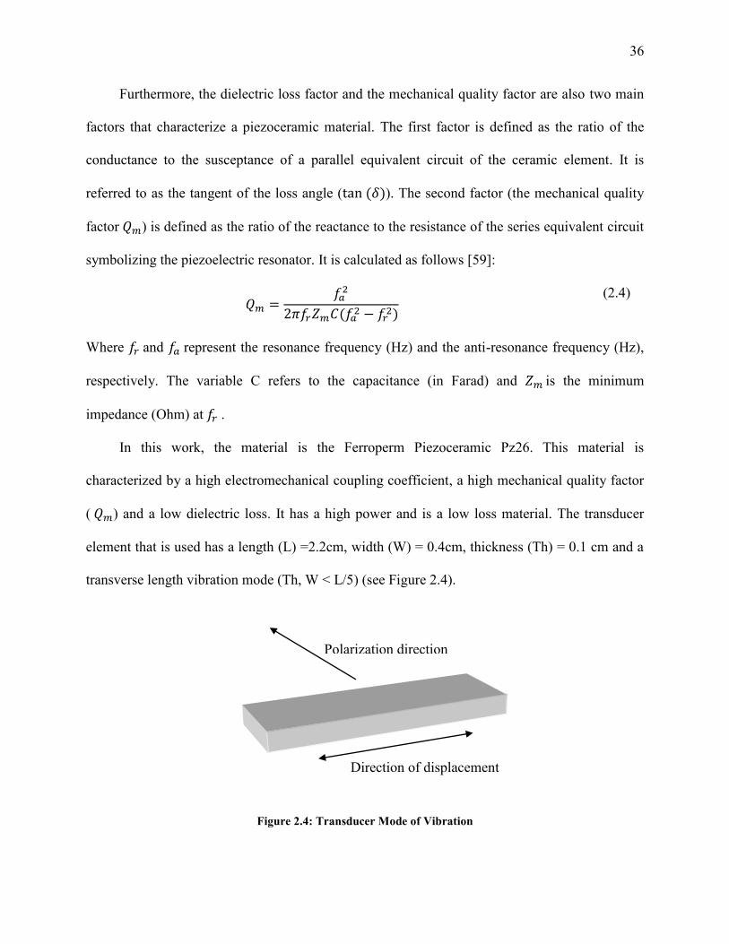
Furthermore, the dielectric loss factor and the mechanical quality factor are also two main
factors that characterize a piezoceramic material. The first factor is defined as the ratio of the
conductance to the susceptance of a parallel equivalent circuit of the ceramic element. It is
referred to as the tangent of the loss angle ( ). The second factor (the mechanical quality
factor ) is defined as the ratio of the reactance to the resistance of the series equivalent circuit
symbolizing the piezoelectric resonator. It is calculated as follows [59]:
(2.4)
Where and represent the resonance frequency (Hz) and the anti-resonance frequency (Hz),
respectively. The variable C refers to the capacitance (in Farad) and is the minimum
impedance (Ohm) at .
In this work, the material is the Ferroperm Piezoceramic Pz26. This material is
characterized by a high electromechanical coupling coefficient, a high mechanical quality factor
( ) and a low dielectric loss. It has a high power and is a low loss material. The transducer
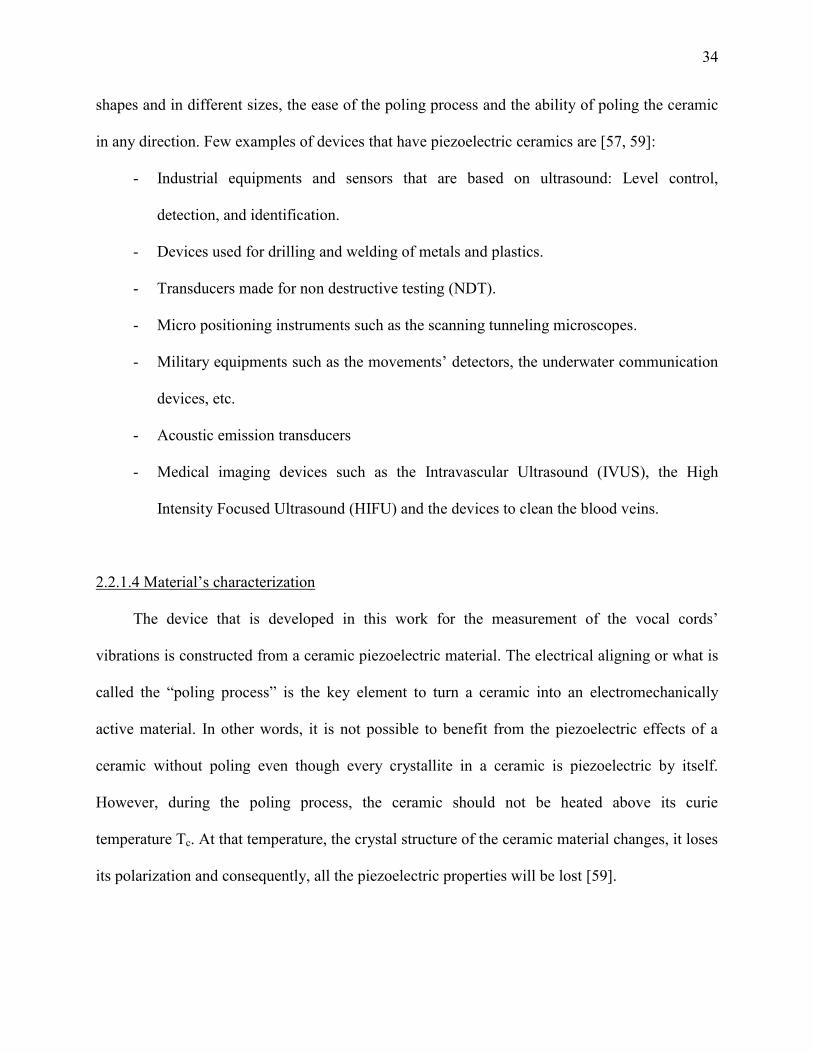
element that is used has a length (L) =2.2cm, width (W) = 0.4cm, thickness (Th) = 0.1 cm and a
transverse length vibration mode (Th, W < L/5) (see Figure 2.4).
Figure 2.4: Transducer Mode of Vibration
Polarization direction
Direction of displacement
Page 47
37
For the transverse mode, the frequency constant (Fc) that represents the product of the
resonance frequency and the linear dimension governing the resonance is calculated as follows
[59]:
(2.5)
Where L is the length of the transducer element. The piezoelectric coupling coefficient (k), for
the transverse length vibration mode, is expressed as follows [59]:
(2.6)
Finally, the elastic compliances are calculated for the transverse mode using the following
equation [59]:
(2.7)
Table 2.1 shows a list of all the material’s characteristics i.e. the electrical properties, the
electromechanical properties and the mechanical properties. All the measurements were done at
a temperature T= 25oC and after 24 hours of the poling process. The tolerances are for the
electrical properties, for the electromechanical properties and for the mechanical
properties and are based on the factory calibration settings [59].
Page 48
38
Table 2.1: Electrical, Electromechanical and Mechanical Properties of PZ26
Dielectric loss factor at 1 KHz ( ) 3 x 10⁻³
Curie temperature (Tc) > 330 oC
Coupling factor (K) 33%
Piezoelectric charge coefficient (q) 130 x 10-12
C/N
Piezoelectric voltage coefficient (g) 11 x 10-3
Vm/N
Frequency constant (Fc) 1500 Hz.m
Density ( ) 7.7 x 10³ Kg/m
3
Elastic compliance (SE) 13 x 10
-12 m
2/V
Mechanical quality factor (Qm) > 1000
2.2.1.5 Methodology
The source of the acoustic energy for the human voice is the glottal cycle [13]. It can be
described as follows: When a person breathes (without speaking), his/her vocal cords in the
larynx are open and the air passes through the lungs easily. However, when he/she speaks,
impulses are transmitted from the brain to the muscles of the larynx conveying a signal to close
the vocal cords. The returning air from the lungs hits the closed vocal cords. The pressure of the
air flow overcomes the resistance of the vocal cords which will be in a rapid vibration state. This
rapid vibration creates the sound waves which propagate in the air and are the basic tones of the
person’s voice [2]. Therefore, the vocal cords constitute the main source of the human voice. In
Page 49
39
this context, the piezoelectric transducer element is attached to a collar that is wrapped around
the subject’s neck. Each individual was requested to utter the vowel “\a\”.
The vocal cords’ vibrations (and the resultant glottal flow signal) constitute the main sound
source for the vocal tract’s excitation during the vowel production [60]. In other words, when
uttering a vowel, the source of the generated sound is mainly the vibrating vocal cords that
transform the steady (DC) airflow from the lower respiratory system into a periodic series of
flow pulses. The latter pulses, known as the glottal flow, are acoustically filtered by the vocal
tract resonances. The latter process harmonizes the frequency components of the source signal
and leads to the generation of the vowel sound. Moreover, the vowel “\a\” reflects the most of
the vocal folds’ vibrations [61].
Having uttered the vowel “\a\”, the vocal cords’ mechanical vibrations were detected by
the transducer attached to the collar and were transformed into an electrical signal to be
processed. The transducer element was connected to the input port of a NI Elvis II+ board (16-bit
resolution). The resulting electrical signal was read by Labview using a sampling frequency of
2500 Hz. Thus, the individual’s signal of the vocal cords’ vibrations is detected and can be
processed.
2.2.2 Short Time Fourier Transform
The acquired signal of a particular individual is a non-stationary signal. Its properties
change substantially over time and the changes are usually of primary interest for analysis and
differentiation purposes. The spectral analysis techniques such as the Fourier Transform provide
a good description of the frequencies’ contents of the waveform but not their timing. The latter
information is encoded in the phase portion of the resulted transform. However, the encoding is
Page 50
40
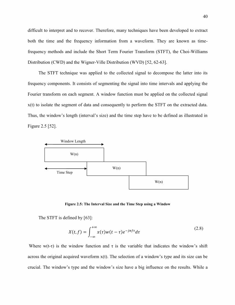
difficult to interpret and to recover. Therefore, many techniques have been developed to extract
both the time and the frequency information from a waveform. They are known as time-
frequency methods and include the Short Term Fourier Transform (STFT), the Choi-Williams
Distribution (CWD) and the Wigner-Ville Distribution (WVD) [52, 62-63].
The STFT technique was applied to the collected signal to decompose the latter into its
frequency components. It consists of segmenting the signal into time intervals and applying the
Fourier transform on each segment. A window function must be applied on the collected signal
x(t) to isolate the segment of data and consequently to perform the STFT on the extracted data.
Thus, the window’s length (interval’s size) and the time step have to be defined as illustrated in
Figure 2.5 [52].
Figure 2.5: The Interval Size and the Time Step using a Window
The STFT is defined by [63]:
(2.8)
Where w(t-τ) is the window function and τ is the variable that indicates the window’s shift
across the original acquired waveform x(t). The selection of a window’s type and its size can be
crucial. The window’s type and the window’s size have a big influence on the results. While a
W(n)
W(n)
Window Length
Time Step
W(n)
Page 51
41
small window’s size improves the time resolution, the frequency resolution will be reduced and
vice versa. Moreover, low frequencies might be lost when the size of the window is very small
because they will not be included in the data segment to be analyzed. Different windows
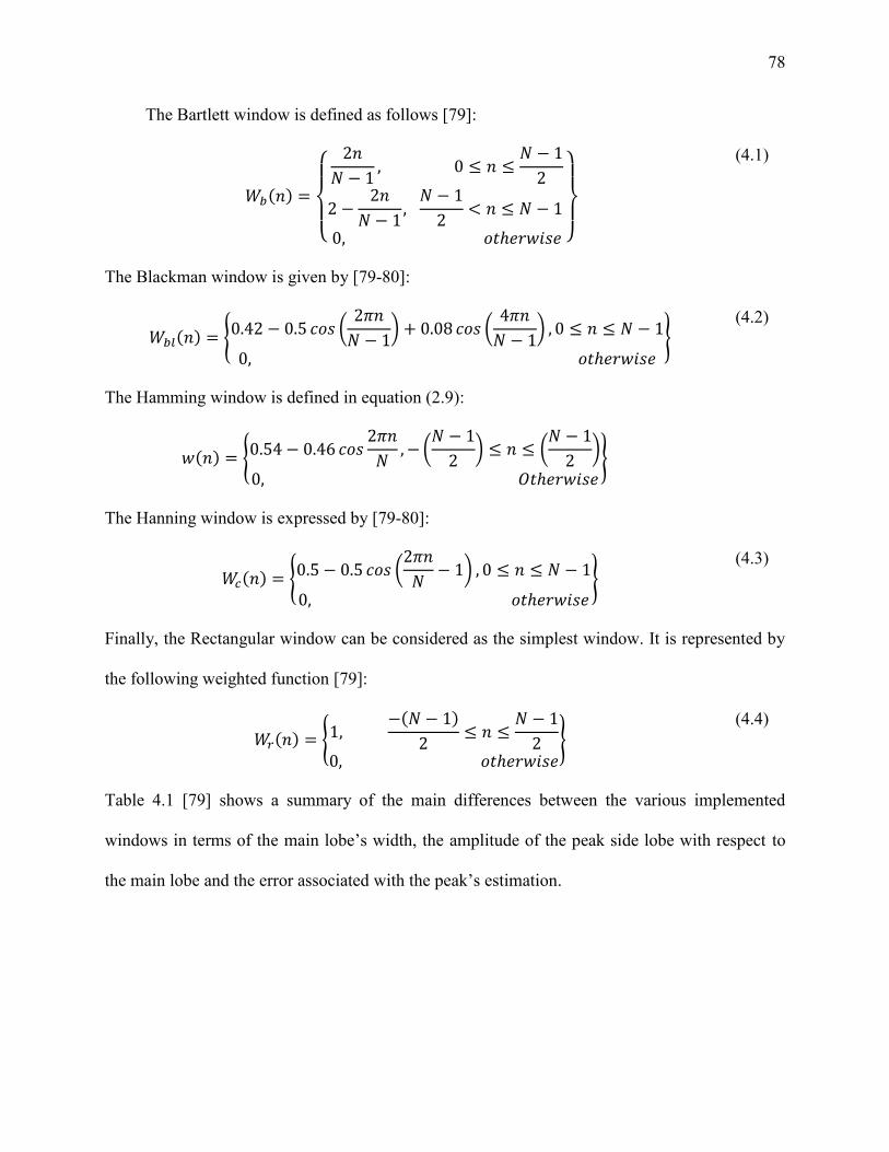
(rectangular, triangular, hanning …) can be applied in conjunction with the STFT. The Hamming
window has been incorporated and can be defined as follows [52]:
(2.9)
2.2.3 Normalization and Noise Removal
The frequencies’ magnitudes are affected by the loudness of the voice i.e. they vary from
one time to another even if the phrase or the word is spoken by the same person. Therefore, they
were normalized by dividing each value by the highest value in order to have the same level for
all subjects under examination.
Having performed the normalization procedure, the magnitudes corresponding to the low
frequencies affect the accuracy of the identification system. They can be considered as noise that
needs to be eliminated or reduced. Therefore, all frequencies which are below a threshold value
are eliminated i.e. their corresponding magnitudes are set to a value of zero.
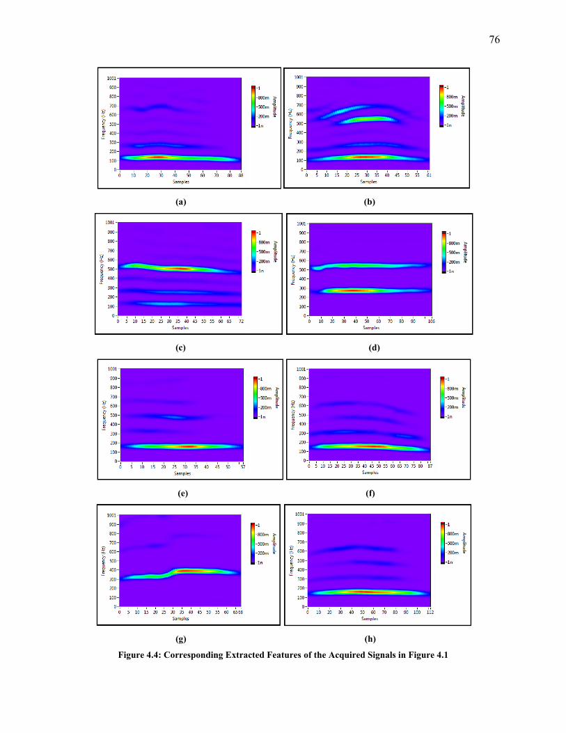
2.2.4 Features’ extraction
The next step involves the extraction of meaningful signal’s frequencies for identification
purposes. A threshold value is selected to be a certain percentage of the maximum amplitude.
The frequencies that are characterized by magnitudes’ values greater than the threshold value are
extracted. Therefore, there is no need to keep the whole spectrum. The intervals that contain the
Page 52
42
necessary information (i.e. the frequencies) are only kept and are stored for comparison and
identification purposes. The extracted features were transformed into a 1-D array for
classification purposes.
2.2.5 Database
The identification process requires the existence of a database in which a template of the
features’ vector of each individual to be identified is stored. In this work, the database consists of
the features’ vectors of N (50) individuals. Actually, each person utters the vowel “a” and the
corresponding signal of the vocal cords’ vibrations is collected. This experiment is repeated three
times for each individual. Thus, 3N signals were collected and each is processed as outlined
before in order to obtain the features’ vector. Then, one features’ vector per individual is stored
in the database and the remaining 2N features’ vectors are used to evaluate the proposed
approach.
2.2.6 Correlation
The linear correlation coefficient Corr(X, Y) between two vectors X and Y is expressed as
[64]:
(2.10)
Where X (a collected features’ vector) and Y (a template features’ vector) are the vectors to be
compared, µx and µy are the mean values of X and Y, respectively, σx and σy are the standard
deviations of X and Y, respectively and rxc is the length of the extracted vector X (or Y). In
each case, the correlation coefficient is calculated between the collected features’ vector and
each one of the N features’ vectors stored in the database. For any two vectors, the closer the
Page 53
43
coefficient’s value is to 1; the higher the similarity is between the two vectors. Then, the highest
correlation value identifies the desired person.
2.2.7 Principal Component Analysis (PCA)
PCA is one of the most famous statistical methods applied for data analysis and
dimensionality reduction. This approach consists of approximating the original vectors of
features by vectors with a lower dimension (i.e. eigenspaces) [65-66]. Thus, the principal idea of
this algorithm is that the new space (i.e. reduced features’ vectors) is characterized by a
dimension that is lower than the dimension of the original extracted features’ vectors.
Consequently, the recognition of the individuals is accomplished in the space of the reduced
dimension. The approach assumes that a training set (database) and a projection matrix (contains
the elements for dimensional reduction) are available. The latter matrix is computed from the
features’ vectors that are stored in the database. The implementation of PCA involves two main
steps: Initialization and Recognition [65].
The initialization step consists of calculating the eigenspaces of the features stored in the
database (training set). The eigenvectors of the covariance matrix highlight the variation that
exists among these features. Thus, each features’ vector of the training set has its respective
contribution or variation incorporated in the computed eigenvectors. Therefore, each vector can
actually be represented as a linear combination of the eigenspaces with the highest eigenvalues.
Then, the weight space of each of the known individuals in the database is calculated by
projecting its corresponding features’ vector on to the eigenspaces. As new measurements are
performed, the computed eigenspaces need to be updated.
Page 54
44
Having initialized the system, the next step involves the classification. The weight of an
input signal is calculated by projecting the input features’ vector onto the stored eigenspaces.
Then, the differences between the new weight and each of the stored weights are calculated. The
smallest difference indicates the highest similarity between the two vectors and the desired
person is identified.
The latter process can be explained mathematically. Let N training features’ vectors be F1,
F2 … FN. Each vector is of dimension (Sx1). The average of the training set is computed by:
(2.11)
The ith feature vector ( ) differs from the average by the vector:
(2.12)
Having adjusted the mean of each vector of the training set, the corresponding covariance matrix
is calculated using the following formula:
(2.13)
Where
(2.14)
The size of the computed covariance matrix C is (SxS). Since the approach requires the
determination of the Eigen values and the corresponding eigenvectors, the complexity of the
computation will be tremendous. Consequently, an alternative covariance matrix that will result
in the same most significant eigenvectors and Eigen values would be more practical to
implement. That is, a computationally feasible method is suggested by Turk and Pentland [67].
The covariance matrix of size N by N can be computed. That is, the covariance matrix XTX
Page 55
45
instead of XXT is considered and it is an N by N matrix. This matrix yields the same most
significant eigenvectors as the previous covariance matrix. Thus, a L matrix is formed as:
(2.15)
The N eigenvectors are calculated from the L matrix and are stored in a vector U of size (NxN)
according to the corresponding eigenvalues organized in descending order. Then, the
eigenspaces vector V is calculated by:
(2.16)
Finally, the weight space is computed as follows:
(2.17)
Similarly, the weight of each new input features’ vector (Finput) is calculated i.e.:
(2.18)
In order to compute the similarity between the input weight vector and the weight of each vector
in the training set, the euclidean distance is used:
(2.19)
Where K = 1, 2….N. The minimum Euclidean distance indicates the highest similarity.
2.3 Conclusion
A non-invasive technique to measure the vocal folds’ vibrations is presented. The
technique consists of attaching a piezoelectric transducer element on a collar and the latter is
wrapped around the person’ neck. The acquired signal is the input to a new developed “text-
dependent” speaker identification system. The developed approach can be summarized as
follows: The Short Time Fourier Transform (STFT) is applied on the collected signal to
decompose it into its frequencies’ contents. Then, the magnitudes of the frequencies are
Page 56
46
normalized by dividing each value by the highest value in order to have a maximum level of 1
for all the subjects under examination. The noise interference is eliminated and the appropriate
features (frequencies) are extracted from each spectrogram. The identification of the speaker is
performed using two evaluation criteria, namely, the correlation similarity measure and the
Principal Component Analysis (PCA) in conjunction with the Euclidean distance.
However, the position of the transducer on the individual’s neck may greatly affect the
quality of the collected signal and consequently the extracted information (i.e. frequencies).
Thus, the search for the best position to place a particular transducer on the individual’s neck is
in accordance. Subsequently, this will ensure to receive the best signal for analysis purposes.
Thus, in the next chapter, the multilayered medium in which the sound propagates before
reaching the surface of the neck is modeled. The structure was assumed to be composed of two
main layers: the fat and the skin. The position of the transducer is examined using Monte Carlo
simulation techniques and consequently, the simulation results are verified using real
experiments.
Page 57
47
CHAPTER 3
MODEL OF THE LAYERS OF THE HUMAN NECK
3.1 Introduction
The vocal cord consists of three main layers: the mucosa, the vocal ligament and the
underlying muscle. The composite microanatomy allows the soft and the flexible superficial
mucosal layers to vibrate freely over the stiffer structural underlayers. The mucosa of the vocal
cord is characterized by its vibratory role and is composed of several layers: the squamous
epithelium, the most superficial layer, and the three layers of lamina propria, each with an
increasing stiffness. The Superficial layer of the Lamina Propria (SLP) is mostly acellular and
consists of extracellualar matrix proteins, water, and loosely arranged fibers of collagen and
elastin. It has a gelatinous nature. The potential space between the SLP and the Intermediate
layer of Lamina Propria (ILP) is the Reinke’s space. The ILP and the Deep layer of the Lamina
Propria (DLP) are composed mostly of elastin and collagen fibers. The densest DLP layer is
formed of tightly arranged collagen fibers. Both, the ILP and the DLP layers constitute the vocal
ligament. The gelatinous superficial layer of the lamina propria and the squamous epithelium,
move freely over the underlying vocal ligament and the muscle to generate the vibrations which
produce the sound [68]. The produced sound propagates as an audible mechanical wave of
pressure and displacement through the layered media of the human neck.
The topic of elastic wave’s propagation in a layered media is widely discussed in the
literature and has been the interest of researchers for many decades. This is due to the large
number of its applications in different domains such as the seismology, the science of acoustics,
and the Non Destructive Examination (NDE) processes [69]. In this context, several methods
have been developed such as the transfer matrix method [70], the delta matrix method [71], the
Page 58
48
global matrix method [72], the recursive stiffness matrix method [69], etc. These methods are
based on different concepts to study the wave propagation in a layered medium and to calculate
the reflection and transmission coefficients.
The recursive stiffness matrix method, defined in [69], is a robust method. The recursive
algorithm is developed to construct the total stiffness matrix as a global banded matrix. The
algorithm deals with the total stresses and the displacements at the interfaces between the layers
instead of building the reflection/transmission matrices. The method’s computation time is
proportional to the number of layers N (same as the standard transfer matrix approach).
However, the limitations of the transfer matrix method with respect to the instability of the
layers’ thicknesses of several wavelengths are addressed. Thus, the recursive stiffness matrix
method is implemented in this work. However, it is adjusted since the medium under study is
considered an isotropic medium (not anisotropic). The simulated model consists of a multilayer
media: a fluid layer, a solid layer and a fluid layer. The layers’ interfaces are assumed to be
perfect (continuity of displacement and stress). The method implemented is unconditionally
stable and is time efficient to simulate the work at hand.
3.2 System Model
The generated sound passes through a multilayer media before reaching the surface of the
neck where it is detected by a transducer. The structure of the neck consists of two main layers:
the fat and the skin. The fat is considered to be a fluid layer and the skin is assumed to be an
elastic solid layer. The signal of the vocal cords’ vibrations is assumed to be an elastic wave that
is incident on the layered structure as shown in Figure 3.1. The variable I is the incident wave
amplitude forming an angle with the perpendicular to the interface. The variable R refers to
Page 59
49
the component of the incident signal (“I”) which is reflected at the level Zo (the interface
between the Fat and the Skin). The remaining component of the signal is transmitted into the
skin (layer 1). The skin is a solid layer where two types of waves propagate: the longitudinal
waves (L waves) and the transverse or shear waves (T waves). A similar behavior is observed in
the skin to the wave which is propagating until the interface between the skin and the gel (Z1) i.e.
reflection and transmission. Subsequently, Tr is the transmitted signal that is propagating in a
fluid medium (Layer 2) representing the gel that is placed on the human’s neck to enhance the
signal’s detection. This layer (Layer 2) is assumed to have the same properties as the Fat Layer
(Layer 0).
Figure 3.1: A Representation of the Multilayered Structure
The analysis of the propagation of the wave and consequently, the computation of the
reflection and the transmission components is based on the stiffness matrix method, as defined in
[69]. The displacement vector um
at the layer m can be written as the summation of partial
Layer 0: Fat (Fluid)
Layer 1: Skin (Solid)
Layer 2: Gel (Fluid)
Z0
Z1
hs
I R
Tr
Z
X
Page 60
50
waves, where the number of partial waves (n) propagating in a medium depends on the nature or
the type of the medium:
(3.1)
Where
,
T refers to the transpose,
refers to the displacement’s amplitude.
The positive and the negative superscripts refer to the wave propagated in the (+z) and the (-z)
directions, respectively.
The parameter
represents the j’th unit displacement polarization vector
that corresponds to the wave vector . The wave vector
refers to the x projection of the
wave number of the incident wave and is calculated, for all types of partial waves and all types
of mediums, using Snell’s law ( i.e.
m), as follows:
(3.2)
The coordinate system, as shown in Figure 3.1, is chosen so that the (x, z) plane coincides with
the incident plane and consequently, .
The stress vector in the (x-y) plane, parallel to the layer surface, is
expressed as follows:
(3.3)
Page 61
51
Where
is related to by a constant C that depends on the type of each
layer.
A displacements-constraints column vector is formed in order to express the
parameters of each medium (m). It includes the components of the total displacement vector
and the components of the stress vector . It is represented as follows:
(3.4)
Where
is a square characteristic matrix describing the medium,
is a diagonal square matrix whose diagonal elements are ,
is a column vector containing the displacement amplitudes.
The components of the vector vary according to the type of the medium m.
A medium can be bounded by two interfaces i.e. an interface at the top of the medium and
an interface at the bottom of the medium (Solid layer, Figure 3.1). Subsequently, the
displacements at the top layer’s surface (z=zm-1) and at the lower layer’s surface (z=zm) can be
expressed as:
(3.5)
Similarly, the stresses at the top and bottom surfaces of each layer are related to the displacement
amplitudes as follows:
(3.6)
Where
and are matrices whose columns are the displacement polarization normalized vectors
of the plane waves propagating in the layer m along the and directions, respectively,
Page 62
52
and are calculated from and respectively, for each type of medium,
and are square diagonal matrices whose elements are and
respectively,
represents the thickness of the mth
layer.
Since
, the following terms of the diagonal matrices are similar i.e.
. Consequently, the corresponding matrices are the same i.e. .
The layer stiffness matrix Km that relates the stress vector to the displacement vector is
obtained by substituting the amplitude vector from eq. 3.5 into eq. 3.6 i.e.:
(3.7)
The stiffness matrix varies from one medium to another since it depends on the type of the
medium. The layer compliance matrix relates the displacement vector to the stress vector and is
expressed as follows:
(3.8)
As it is stated earlier, the structure through which the wave is propagating is composed of
three layers: a fluid layer, a solid layer and a fluid layer (i.e. the gel). In order to compute the
reflection and the transmission coefficients of the simulated model, the stiffness matrix of the
solid layer needs to be calculated. The characteristic matrix of the fluid layer(s) is needed.
Moreover, the boundary conditions between the mediums have to be taken into account.
Page 63
53
3.2.1 Fluid Layer
The waves which are propagating in the fluid are only of longitudinal type [73]. Therefore,
two longitudinal waves propagate in the (+z) and the (-z) directions. The wave number km
of the
fluid is expressed as:
(3.9)
And, according to eq. 3.2:
(3.10)
Then,
(3.11)
Where
is the angular frequency,
Cf is the speed of sound in the fluid.
The boundary conditions at the interface of a fluid layer express the continuity of the vertical
displacement and the continuity of the fluid pressure [73]. Then, the displacement-constraint
column vector of a fluid is expressed as:
(3.12)
The z component of the displacement vector is expressed as follows:
(3.13)
The unit displacement polarization vectors in the fluid are:
and
Moreover, the dilatation or the pressure (Pr) in the fluid can be defined as:
Page 64
54
(3.14)
Where
represents the bulk modulus of the fluid,
is the density of the fluid,
is the divergence of the vector .
Then, eq 3.4 becomes:
(3.15)
Where is called the 2x2 characteristic matrix of the fluid.
After performing certain manipulations and simplifications, the characteristic matrix is
represented as follows:
(3.16)
Where is the fluid impedance, and is equal to .
3.2.2 Solid Layer
Two types of waves can propagate in an isotropic elastic solid layer: the longitudinal waves
(L waves) and the transverse or shear waves (T waves) [73]. The longitudinal wave number is
expressed as:
(3.17)
Where refers to the speed of the longitudinal wave in the solid. It is computed as follows:
Page 65
55
(3.18)
Where
is the density of the solid,
µ and are the Lamé coefficients.
Then, according to eq. 3.2:
(3.19)
Thus,
(3.20)
Similarly, the wave number of the transverse wave is given by:
(3.21)
Where is the speed of the transverse wave in the solid i.e.
(3.22)
According to eq. 3.2, the wave numbers of the transverse wave become:
(3.23)
And
(3.24)
The boundary conditions at the interface of a solid layer express the continuity of the x and
z components of the displacement and the continuity of each of the (x,z) and (z,z) components of
the stress tensor [73]. Then, the displacements-constraints column vector of a solid is defined as:
Page 66
56
(3.25)
The x and z components of the displacement vector can be expressed as follows:
(3.26)
And
(3.27)
Where
The two angles and refer to the angle of the longitudinal wave and the angle of the
transverse wave with respect to the normal to the interface, respectively.
The stress tensor is expressed as follows:
(3.28)
Where
i and j refer to the axis of the coordinate system (x, y, z),
refers to the Kronecker delta:
(3.29)
is the strain tensor and is given by:
Page 67
57
(3.30)
Then, similar to the fluid layer, the displacements-constraints column vector of a solid can be
formed and is given by:
(3.31)
Where is called the 4x4 characteristic matrix of the solid.
After having performed certain manipulations and simplifications, the characteristic matrix can
be reduced to:
=
(3.32)
To simplify the presentation for further calculations, the latter characteristic matrix is divided
into 4 equal (2x2) sub matrices i.e.:
(3.33)
Page 68
58
The solid layer’s stiffness matrix is formed by relating the (x, z) and the (z, z) components
of the stress tensor to the x and z components of the displacement vector, respectively:
(3.34)
Based on eq. 3.7, is given by:
(3.35)
Where
,
i.e. the thickness of the solid layer (Figure 3.1).
3.2.3 Fluid-Solid Interface
The continuity conditions at the fluid-solid interface are given by [73]:
(3.36)
The same conditions apply at the second interface (solid-fluid):
(3.37)
3.2.4 Reflection and Transmission Coefficients
The reflection coefficient (R) in the first layer (Layer 0) and the transmission coefficient
(Tr) in the third layer (Layer 2) are calculated (Figure 3.1). It is to be noted here that the
Page 69
59
refracted angles in the various mediums are related, according to Snell’s law [74-75], by the
following equation:
(3.38)
Since Layer 0 and Layer 2 are identical, . Also, they have the same characteristic matrix
[G]. Furthermore, before proceeding with the calculations, it is to be noted that the term
is omitted since it will be simplified in the calculations.
The fist layer (Layer 0) is a fluid. The amplitude of the incident wave (I) is assumed to be
equal to one. The terms ( and ) are neglected at the first layer and at the last layer
(known also as the first semi space and the last semi space) since they are not bounded by two
interfaces [69]. Then, eq. 3.15 becomes at Z0=0 (origin of the Z axis) as follows:
(3.39)
This will give:
(3.40)
Since layer 2 is the last layer, it is the layer in which the signal is detected i.e. the transmitted
wave (Tr). Therefore, there is no reflection (i.e. ). Then, at layer 2 (Z=Z1) eq. 3.15 yields:
(3.41)
Consequently, eq. 3.41 can be written as:
(3.42)
Page 70
60
Moreover, the displacements and stresses at the top interface of the solid layer (at Z=Z0)
are related to the displacements and stresses at the bottom interface of the layer (Z=Z1) by the
solid stiffness matrix described earlier. The compliance matrix of the solid layer (denoted
by ) is equal to (eq. 3.8). By using the compliance matrix instead of the stiffness
matrix, eq. 3.34 leads to:
(3.43)
After applying the boundary conditions (eq 3.36 and eq. 3.37), the following equations can be
extracted from eq. 3.43:
(3.44)
The substitution of eq. 3.40 and eq. 3.42 into eq. 3.44 yields:
(3.45)
The above system can be written in a matrix form i.e.:
(3.46)
It is a linear system that can be solved using linear algebra for a unique solution i.e. of the
transmission and the reflection coefficients:
(3.47)
3.2.5 Results
The signal of the vocal cords is generated when an individual speaks. It propagates in the
multilayered medium illustrated in Figure 3.1. It is a non-stationary signal and it contains
Page 71
61
different frequencies. Moreover, its range of frequencies varies from an individual to another.
The signal of the vocal cords’ vibrations is acquired by attaching the transducer to the subject’s
neck using a collar. Subsequently, the collected signal is processed and analyzed. The position of
the transducer may greatly affect the collected signal and consequently the results for
identification and classification purposes in medical and non medical applications. Thus, there is
a need to find the best position on the individual’s neck to place a particular transducer in order
to receive the best signal for analysis and/or diagnostic purposes. In this context, the position of
the transducer is investigated using Monte Carlo simulation techniques and the simulation results
are verified using real experiments. It is to be noted that the position of the transducer can be
defined in terms of the angle with respect to the normal at the interface i.e. the longitudinal axis
(Z-axis).
In order to examine the best location, an incident acoustic signal with a particular
frequency and a particular incident angle is generated. Then, the generated beam propagated
through the fat medium, the skin medium and another liquid medium (gel). At this point, the
transmission coefficient or/and the corresponding reflection coefficient are computed. Then,
another sound signal is generated with a different frequency and the same incident angle. The
corresponding transmission coefficient or/and reflection coefficient are estimated as it is
illustrated earlier. This Monte-Carlo (MC) simulation experiment is performed for a range of
frequencies for the same angle .
Having completed the experiments with a particular incident angle and for a range of
frequencies, the MC experiments are repeated for a different incident angle and the same range
of frequencies. Actually, the MC experiments are performed for a range of incident angles. For
each simulated experiment, the corresponding transmission coefficient is computed. Thus, a set
Page 72
62
of values of the transmission coefficient is obtained for a range of and a range of frequencies.
Table 3.1 shows the values of the main parameters that were taken into consideration in the MC
simulation experiments for the fluid medium and the solid medium [76-77]. The best incident
angle (i.e. the angle that yields the highest transmission coefficients for all frequencies) will be
the best angle at which the signal of the vocal cords’ vibrations can be acquired. Consequently,
the best transmission angle (since as illustrated earlier, eq. 3.38). Thus, that will be
the best position to attach the transducer on the neck using a collar.
Table 3.1: Basic Parameters of the Fluid and the Solid layers
Fluid Density ( ) 920 Kg.m-3
Speed of sound in fluid (Cf) 1450 m.s-1
Solid Thickness (h) 2 mm
Density ( ) 1050 Kg.m-3
µ 2.1 Mpa
50.4 Mpa
The incident angle is assumed to vary from 0o to 90
o with an increment of 1
o. Similarly,
the frequency of the generated sound is assumed to vary from 0 to 2 KHz with an increment of 1
Hz. Even though the frequencies of the vocal cords’ vibrations are normally within the range
50Hz-1000Hz, the maximum frequency is equal to a value of 2 KHz for consistency and
completeness of the work.
Figure 3.2 shows the reflection/transmission coefficients in function of the incidence angle
and the frequency f for various MC simulation experiments. It shows an intensity plot of the
Page 73
63
incident angle (i.e. the transmission angle in layer 2) versus the frequency of the generated
signal. The pure black color indicates a maximum transmission while the pure white color
indicates a total reflection (zero transmission). The results show that there is practically a good
transmission for almost all the incident angles. However, if the incident angle is between 70o and
90o, the transmission is low for high frequencies. In other words, the frequencies that are above
300 Hz might be altered or even are not detected. Moreover, there is no transmission of the
incident signal if the incident angle is between 87o and 90
o for all range of frequencies which are
simulated in these experiments. Therefore, it is not recommended to attach a transducer inside
that region (i.e. [70o 90
o]). The latter point is illustrated experimentally in the next section.
Furthermore, it can be noted that for a given incident angle ( for example), the
intensity of the transmission (intensity of the black color) decreases as the frequency increases
for frequencies above 1 KHz. Similarly, for a given frequency (f = 0.8 KHz for example), the
intensity of the transmission decreases as the incident angle increases for incident angles
above . However, if the incident angle is in the range [50o 70
o], the black color stills the
dominant color and consequently, a good transmission can be achieved.
The highest transmission coefficients which are observed correspond to an incident angle
in the range of [0o 70
o]. This can be referred to as the safe region in which the transducer element
can be attached. These theoretical MC simulations were performed to locate the regions of
maximum sensitivity (in terms of frequency and incident angle) in order to detect the signal of
the vocal cords’ vibrations after its propagation through the multilayered structure of the
human’s neck.
Page 74
64
Figure 3.2: Reflection/Transmission Coefficients in function of [f, θ] for a Multilayer of 3 Layers
3.3 Experimental Evaluation
As it is mentioned earlier, a piezoelectric transducer element is built and is attached on a
collar that is wrapped around the neck of subjects. The transducer that is constructed from a
piezoelectric material generates a charge when a pressure is applied on its surface. The person is
requested to utter the vowel ‘a’. The vocal cords’ vibrations at the moment of uttering the vowel
were detected by the transducer element and were transformed into an electrical energy. The
transducer element was connected to the input port of a NI Elvis II+ board (16-bit resolution).
The resulting electrical signal was read through the software labview using a sampling frequency
of 2500 Hz.
Page 75
65
For each individual, three signals (speaker uttering the vowel ‘a’) were recorded. The first
signal was collected by attaching the transducer around the neck inside the region that is defined
by the angle 20o and the angle 30
o with respect to the normal to the laryngeal prominence. The
second measurement was collected by placing the transducer around the neck inside the region
that is defined by the angle 50o and the angle 60
o. The third measurement was performed with
the transducer located in the region bounded by the angles 75o and 85
o. The collected signals are
non stationary signals. They are analyzed using the proposed time-frequency approach (i.e.
STFT) in order to extract the existing frequencies and their respective time of occurrence. Figure
3.3 and Figure 3.4 show three detected signals of an individual “A” and an individual “B”,
respectively, as well as the corresponding spectrograms using the Short Time Fourier Transform
(STFT) in conjunction with a Hamming window of size 64 and a time step of 5. The frequencies
shown in each spectrogram represents the frequencies of the vocal cords’ vibrations (50Hz-
1000Hz) of the individual which are detected by attaching the transducer on the subject’s skin in
the corresponding defined bounded region.
Page 76
66
(a) (b)
(c) (d)
(e) (f)
Figure 3.3: Three Signals for an Individual “A” are acquired by placing the Transducer in the Region
bounded by (a) the Angles 20o and 30
o, (c) the Angles 50
o and 60
oand (e) the Angles 75
o and 85
o. The
Corresponding Spectrograms are illustrated in the plots (b), (d) and (f), respectively.
Page 77
67
(a) (b)
(c) (d)
(e) (f)
Figure 3.4: Three Signals for an Individual “B” are acquired by placing the Transducer in the Region
bounded by (a) the Angles 20o and 30
o, (c) the Angles 50
o and 60
oand (e) the Angles 75
o and 85
o. The
Corresponding Spectrograms are illustrated in the plots (b), (d) and (f), respectively.
Page 78
68
The results show:
(i) The spectrograms shown in the subplots (b) and (d) of Figures 3.3 and 3.4 contain more
information than the spectrograms shown in the subplots (f) of Figures 3.3 and 3.4. They show
ranges of frequencies that are associated with the person’s voice and were not detected in the
spectrograms of Figure 3.3-f and Figure 3.4-f.
(ii) In the latter context, the high frequency components (>400 Hz) that were detected in
the two spectrograms of Figures 3.3-b and 3.3-d are not detected (or weakly or improperly
detected) in the spectrogram of Figure 3.3-f. Similarly, the frequencies around 600 Hz in Figures
3.4-b and 3.4-d are not detected in Figure 3.4-f.
(iii) The real experimental results are in accordance with the theoretical study that is
performed using Monte Carlo simulation techniques. That is, the transducer should be attached
in the region corresponding to ]0o 70
o] and the region above 70
o should be avoided.
Subsequently, the high frequencies’ components existing in a signal might be lost when the
incident angle is in the interval [70o 90
o].
3.4 Conclusion
In this chapter, Monte Carlo simulation techniques were performed in order to determine
the best transmission area on the human neck i.e. the best area to place a transducer in order to
have a good detection of the vibrations’ signal of the human vocal cords. The layers of the
human neck were modeled and the reflection/transmission coefficients of the transmitted signal
were computed. The results have shown that there is practically a good transmission for almost
all incident angles. However, if the incident angle is in the interval [70o 90
o], the transmission is
low for the frequencies that are above 300 Hz. Therefore, it is not recommended to attach a
Page 79
69
transducer in that location or region. The above results are further proven by performing real
experiments i.e. by collecting the vocal cords’ signal by placing the transducer in various
regions. As result, the region bounded by the angles [0o 70
o] with respect to the normal to the
laryngeal prominence is proved to be the best location to place a transducer.
Since the detected frequencies of the speaker’s voice are different for different individuals,
they can be a basis to identify the person by analyzing the collected signals. Furthermore, they
can be used for the recognition of a specific pathology in the speaker’s (patient) voice since
several pathologies affect the frequencies of the vocal cords’ vibrations.
Page 80
70
CHAPTER 4
RESULTS AND PERFORMANCE EVALUATION
4.1 Introduction
In this chapter, the performance of the proposed text-dependent speaker identification
system is being evaluated quantitatively by studying its accuracy using the correlation similarity
measure and also using the PCA in conjunction with the Euclidean distance as a similarity
measure. Besides, the effect of the window’s type, the window’s size and the time step on the
identification accuracy is also investigated. Also, other time-frequency techniques are
implemented and the results are compared with the results of the developed approach.
4.2 Method
The prototype equipment was wrapped around each individual’s neck and the individual
was requested to utter the vowel “\a\”. The transducer element was connected to the input port of
a NI Elvis II+ board (16-bit resolution). The resulting electrical signal was read by labview and
was stored in a file for analysis and comparison purposes. Samples were collected from N (=50)
individuals, under noisy conditions (people talking in the background), and using a sampling
frequency of 2500 Hz. Figure 4.3 shows the detected signals of eight different individuals
uttering the vowel “\a\”. It is clearly evident that the collected signals in time domain show a
certain variation between them.
Having acquired the signal of the vocal cords’ vibrations, the signal is processed using the
STFT technique in conjunction with the Hamming window. The corresponding spectrograms of
the eight individuals are illustrated in Figure 4.2. The window’s size is selected to be 64 with a
time step of 5. The amplitudes of the existing frequencies are represented by different colors.
Page 81
71
(a) (b)
(c) (d)
(e) (f)
(g) (h)
Figure 4.1: Acquired Signals for eight different Individuals
Page 82
72
(a) (b)
(c) (d)
(e) (f)
(g) (h)
Figure 4.2: Corresponding Spectrograms of the Eight Acquired Signals in Figure 4.1
Page 83
73
It is clearly evident that the eight spectrograms are different. That is, the frequencies’
content of each spectrogram does not resemble any other. Therefore, this observation highlights
the possibility of differentiating between the various individuals and consequently, the extracted
features should form the basis of the identification between them. Besides, a difference in
frequencies’ magnitudes between the spectrograms can be observed. That is, the amplitudes’
range of the frequencies is from 100 atto to 100 nano in Figure (4.2-a), while the amplitudes’
range is in the interval [20 atto, 20 nano] in Figure (4.2-b). Similarly, the magnitudes of the
frequencies in each of the remaining spectrograms vary within a certain interval which is
completely different from the other intervals. Thus, a normalization procedure is in accordance
in order for all spectrograms to have the same maximum magnitude and consequently, to
eliminate the effect of the magnitude on the identification’s accuracy. The normalization
procedure is achieved by dividing the values of each spectrogram by the corresponding
maximum amplitude. At this stage, the frequencies’ magnitudes of each spectrogram have a
maximum value of one.
The next step is to eliminate the noise. The low frequency components that are observed at
the bottom of some spectrograms are mostly the result of noise interference (such as body
movement near the contact surface of the collar) and consequently, they should be eliminated in
order to achieve a better accuracy, even though these components might have a quite high
magnitude’s value. These frequency components are not the results of the utterance of the vowel
“\a\” i.e. frequencies associated with. This phenomenon is evident in the spectrograms illustrated
in Figure 4.2-b and Figure 4.2-g i.e. the values near or close to the frequency of zero. The
corresponding normalized spectrograms after removing the “noise” are shown in Figure 4.3.
Page 84
74
(a) (b)
(c) (d)
(e) (f)
(g) (h)
Figure 4.3: Spectrograms of the acquired signals in Figure 4.1 after Normalization and Noise Removal
Page 85
75
At this point, the eight spectrograms have the same range of frequencies’ amplitudes and
the low frequency components (i.e. “noise”) are removed. Each spectrogram is effectively a 2-D
array containing the magnitudes’ values of the frequencies. There is no need to keep the whole
array since these frequencies exist only in certain ranges of the spectrogram. Therefore, the
frequencies of interest existing in each spectrogram are extracted. A threshold value
corresponding to 20% of the maximum amplitude is selected. Then, the extraction is performed
by selecting a range from the 2-D array bounded by two vertical lines. While the first line
corresponds to the first sample’s index associated with the frequency component having a
magnitude value greater than the threshold value, the second line corresponds to the last
sample’s index associated with the frequency component having a magnitude value greater than
the threshold value. All the frequencies of interest will be inside the selected range of the
spectrogram. The results are shown in Figure 4.4. Furthermore, the latter figure illustrates clearly
the difference in frequencies’ contents among the eight individuals. Subsequently, the extracted
features that are associated with each individual can form the basis for identification purposes.
Page 86
76
(a) (b)
(c) (d)
(e) (f)
(g) (h)
Figure 4.4: Corresponding Extracted Features of the Acquired Signals in Figure 4.1
Page 87
77
Each resulting spectrogram (2-D array) is transformed (row by row) into a 1-D vector of
length S= rxc (r=502, c=1002). The length of the feature vector will be the same for all
individuals. By referring to Figure (4.4-a) as an example, the first entries of the feature vector are
filled with the extracted information (length 88x1002) and the remaining entries are padded with
zeros. One feature vector for each individual was stored in the database (training set) and the
remaining acquired feature vectors (or signals) were used to study the performance of the
proposed approach. The system can be referred to as a closed set speaker identification system,
i.e. N speakers with N alternative decisions [78]. The input speech is classified as one of the N
speakers. The classification is achieved using the correlation similarity measure and also by
implementing the PCA algorithm along with the Euclidean distance. The results show that the
proposed PCA based approach achieved a precision of 92% in identifying the right individual in
comparison with a 91% for the correlation based approach.
4.3 Effect of the Window
As it is already stated earlier, the proposed time-frequency based approach involves the
implementation of STFT in conjunction with a particular window. Subsequently, different
windows can be incorporated and their effects can be studied and evaluated i.e. the dependence
of the performance of the proposed approach on the window’s type and its size. In this context,
various windows, namely, the Bartlett, the Blackman, the Hamming, the Hanning and the
Rectangular are implemented in conjunction with the proposed technique and their effects on the
precision of the developed approach and the accuracy in the identification of the desired
individuals were studied. The various windows are presented before proceeding to the
quantitative analysis.
Page 88
78
The Bartlett window is defined as follows [79]:
(4.1)
The Blackman window is given by [79-80]:
(4.2)
The Hamming window is defined in equation (2.9):
The Hanning window is expressed by [79-80]:
(4.3)
Finally, the Rectangular window can be considered as the simplest window. It is represented by
the following weighted function [79]:
(4.4)
Table 4.1 [79] shows a summary of the main differences between the various implemented
windows in terms of the main lobe’s width, the amplitude of the peak side lobe with respect to
the main lobe and the error associated with the peak’s estimation.
Page 89
79
Table 4.1: Comparison of Windows’ Parameters
Window Type
Approximate
Amplitude of the
Peak Side Lobe
Approximate Main
Lobe’s Width
Peak Estimation
Error (dB)
Barlett -25
-25
Blackman -57
-74
Hamming -41
-53
Hanning -31
-44
Rectangular -13
21
The main parameter that affects the efficiency of a window is the width of the main lobe.
The latter is directly related to the frequency resolution of the windowed signal. Therefore, the
ability to distinguish two closely spaced frequency components increases as the main lobe of the
window becomes narrower. However, as the main lobe of the window becomes narrower and the
spectral resolution improves, the window’s energy spreads into the side lobes. This increases the
spectral leakage and decreases the amplitude accuracy [81]. Then, a trade-off between the
amplitude’s accuracy and the spectral resolution should be taken into consideration when
choosing the appropriate window to implement. Moreover, it can be noted from Table 4.1 that as
the amplitude of the peak side lobe with respect to the main lobe decreases, the error associated
with the peak’s estimation decreases.
Table 4.2 illustrates the accuracy of the proposed technique in conjunction with the
different windows’ types, namely, the Barlett, the Blackman, the Hamming, the Hanning and the
Rectangular and using various windows’ sizes, namely, 32, 64, 128, 256, and 512. The step size
is selected to be 5. The accuracy is measured in terms of the number of individuals that are
Page 90
80
identified correctly (i.e. the percentage of correct identification). The identification of the
individuals is based on the PCA and the Euclidean distance as a similarity measure. Similarly,
Table 4.3 shows the results of the correlation based approach i.e. the correlation similarity
measure is used to recognize a desired person. It is to be noted that the two tables are the results
of the implementation of the proposed approaches illustrated in Figures 2.1 and 2.2, respectively.
Table 4.2: Percentage of Accuracy of the Proposed Technique Using PCA and Euclidean Distance in
Identifying the Desired Individual for Different Window’s Types and Window’s Sizes
Window’s Type
Window’s Size 32 64 128 256 512
Barlett 73 86 79 71 66
Blackman 65 86 83 74 69
Hamming 77 92 79 70 62
Hanning 73 86 81 71 69
Rectangular 89 83 75 68 65
Table 4.3: Percentage of Accuracy of the Proposed Technique Using the Correlation Similarity Measure in
Identifying the Desired Individual for Different Window’s Types and Window’s Sizes
Window’s Type
Window’s Size 32 64 128 256 512
Barlett 76 88 79 70 66
Blackman 62 85 85 72 69
Hamming 77 91 79 69 64
Hanning 73 87 81 70 66
Rectangular 88 86 74 67 65
Page 91
81
The results that are presented in both tables show:
i) The implementation of the STFT technique in conjunction with a Hamming window of
size 64 yields the best performance i.e. 91% with correlation and 92% with PCA.
ii) For a given window, the accuracy of the proposed approach in identifying the
individuals decreases as the size of the window increases (for window’s size ≥ 64). The decrease
that is observed might be due to the fact that as the size of the window is increased, the varying
nature of the collected signal might be affected in the frequency domain.
iii) For a window’s size of 32, the precision of the approach using the various windows is
not high. This might be due to the fact that the small window’s size does not contain enough
information that leads to a higher percentage of identification.
iv) The percentages obtained using the correlation and the PCA are comparable and a
better performance is achieved by the PCA based approach. That is, it is clear that the PCA has
yielded a higher percentage of accuracy for 11 cases (i.e. combinations of window’s type and
window’s size); while the correlation based approach has achieved a better performance for 6
cases. In 8 cases, both approaches had the same percentage of accuracy in correctly identifying
the individuals. However, the best performance is achieved by the proposed PCA based approach
as illustrated in (i).
The above conclusion can be further proved qualitatively i.e. a qualitative analysis can be
performed with respect to the window’s size by simply visualizing the spectrogram of an
individual using a particular window for various sizes of the window. Figures 4.5, 4.6, 4.7, 4.8
and 4.9 show the spectrograms of two individuals (individual ‘A’ and individual ‘B’), after the
procedures of the normalization and the noise removal are implemented, using a hamming
window with various sizes, namely, 32, 64, 128, 256 and 512, respectively.
Page 92
82
(a) (b)
Figure 4.5: Spectrograms after Normalization and Noise Removal using a Hamming Window of Size 32
(a) (b)
Figure 4.6: Spectrograms after Normalization and Noise Removal using a Hamming Window of Size 64
(a) (b)
Figure 4.7: Spectrograms after Normalization and Noise Removal using a Hamming Window of Size 128
Page 93
83
(a) (b)
Figure 4.8: Spectrograms after Normalization and Noise Removal using a Hamming Window of Size 256
(a) (b)
Figure 4.9: Spectrograms after Normalization and Noise Removal using a Hamming Window of Size 512
The results seen in the spectrograms are in accordance with the quantitative analysis that is
performed earlier. First, the frequency’s contents in each spectrogram are not the same when
varying the window’s size. That explains the different percentages of accuracy obtained earlier.
Second, for small window’s size (window of size 32), the frequency resolution is very poor. In
other words, there is interference between the magnitudes of the frequencies’ components of the
signal. Third, for large window’s sizes (window of size 256 and window of size 512), the
spectrograms are not clear and the frequencies of the signal are not well represented.
Subsequently, this justifies the low percentage of identification’s accuracy when these window’s
sizes are implemented. Fourth, it seems that a window’s size of 64 provides a good frequency
Page 94
84
and temporal resolution and consequently, a high percentage in the identification of individuals
is obtained.
4.4 Effect of the Time Step
In the previous section, various windows with various sizes were incorporated in
conjunction with the proposed time frequency approach to identify the desired person. The best
performance was reached when the size of the window is 64 and 128. In this section, the effect of
the time step on the identification accuracy is investigated and studied. Since the best results
were achieved with the Hamming window, the experiments performed in this section will be
restricted to the latter window. Thus, the proposed approach in conjunction with the Hamming
window with a size of 64 and a size of 128 is examined. The time steps are selected to be 1, 5,
10, 32 and 64. Table 4.3 and Table 4.4 show the performance of the proposed algorithm using
the PCA based approach and the correlation based approach, respectively.
Table 4.4: Percentage of Accuracy of the Proposed Technique (Using the Hamming Window of Sizes 64 and
128) Using PCA and Euclidean Distance as a function of the Time Step
Window 1 5 10 32 64
Hamming of size 64 91 92 91 92 87
Hamming of size 128 79 79 81 78 79
Table 4.5: Percentage of Accuracy of the Proposed Technique (Using the Hamming Window of Sizes 64 and
128) Using the Correlation Similarity Measure as a Function of the Time Step
Window 1 5 10 32 64
Hamming of size 64 90 91 89 90 85
Hamming of size 128 79 79 80 78 78
Page 95
85
The results show that:
i) In each table, the best precision for identification purposes is achieved when the size of
the window is 64. This observation is true for all the tested time steps.
ii) In each table, the precision is decreased when the size of the window is increased for a
given time step.
iii) For a given approach and a given window’s size, the accuracy of identification is
comparable as the step size is increased i.e. the percentages are very close (the difference is less
than 2%). However, the accuracy has shown a certain remarkable decrease as the step size is
increased from 32 to 64 in some cases.
iv) For a given window and a given size, the PCA based proposed approach usually yields
a better accuracy than the correlation based approach and particularly when the window size is
64.
v) In each table, the highest percentage is observed when the window’s size is 64 and the
time step is 5.
To further clarify the effect of the time step, Figures 4.10, 4.11, 4.12, 4.13 and 4.14 show the
spectrograms of the first two acquired signals (individual ‘A’ and individual ‘B’) with a time
step of 1, 5, 10, 32 and 64, respectively. The proposed technique is implemented in conjunction
with a Hamming window of size 64. Each figure displays the corresponding spectrograms after
the procedure of the normalization and the procedure of noise removal are performed.
Page 96
86
(a) (b)
Figure 4.10: Spectrograms (after Normalization and Noise Removal Procedure) using a Hamming Window of
Size 64 and a time step of 1
(a) (b)
Figure 4.11: Spectrograms (after Normalization and Noise Removal Procedure) using a Hamming Window of
Size 64 and a time step of 5
(a) (b)
Figure 4.12: Spectrograms (after Normalization and Noise Removal Procedure) using a Hamming Window of
Size 64 and a time step of 10
Page 97
87
(a) (b)
Figure 4.13: Spectrograms (after Normalization and Noise Removal Procedure) using a Hamming Window of
Size 64 and a time step of 32
(a) (b)
Figure 4.14: Spectrograms (after Normalization and Noise Removal Procedure) using a Hamming Window of
Size 64 and a time step of 64
It is evident that the appearance of the spectrograms deteriorates as the step size is
increased from 1 to 5, 10, 32 and 64. Also, it is clearly observed that some important and useful
information will be lost when the step size is large i.e. 32 and 64. Thus, the quality of the
spectrograms decreases as is clearly seen in Figure 4.13 and Figure 4.14. Consequently, the best
quality is obtained when a small step size is selected i.e. a step size of 1 (Figure 4.10), a step size
of 5 (Figure 4.11) and a step size of 10 (Figure 4.12). However, the quantitative evaluation in
terms of the precision can further identify the best time step i.e. Table 4.5 and Table 4.6.
Page 98
88
Furthermore, as the time step decreases, the spectrogram’s size (i.e. matrix size) increases.
Subsequently, the size of the feature vector will increase. That is, more detailed information will
be included for identification purposes. However, at some point, the added information might not
add any new characteristics. In addition, a large matrix could be computationally time
consuming. Thus, a compromise should be made between the quality of the spectrogram and the
size of the matrix. In this context, a time step of 5 was adopted in this work. Besides, the highest
identification’s accuracy is achieved when a step size of 5 is selected for all windows and for
both proposed approaches i.e. based PCA and based Correlation.
4.5 Evaluation with Other techniques
Having studied the performance of the proposed technique, a quantitative evaluation is
performed by comparing the developed approach with other time-frequency methods, namely,
the Choi-Williams Distribution (CWD) and the Wigner-Ville Distribution (WVD). The time-
frequency analysis is proved to be one of the most effective methods to analyze non-stationary
signals such as the speech. Moreover, the spectrogram is the most common method for speech
analysis. In particular, the CWD and the WVD have been used for feature extraction in many
speaker identification systems existing in the literature [40]. Thus, they were considered for
performance evaluation against the proposed time-frequency approach.
4.5.1 Wigner-Ville Distribution
This technique was first invented by Wigner and was implemented in physics. Then, it was
applied by Ville in signal processing. Hence, the dual name Wigner-Ville Distribution (WVD) is
associated with the transformation. The WVD technique has gained a considerable attention
Page 99
89
lately because of its important role in analyzing non-stationary or time-varying signals. It is a
two-dimensional function that presents the frequency components of a signal as a function of
time. It provides a good resolution and an instantaneous energy density spectrum in the time and
frequency domains (spectrogram) [40, 82]. For a given signal x(t), the WVD is expressed as [63]
:
(4.5)
Where x*(t) refers to the complex conjugate of x(t).
The Wigner distribution provides the energy distribution of the signal as a function of time
and frequency by performing the Fourier transform on the local autocorrelation function of that
signal. It possesses a high time–frequency resolution. The WVD fulfils the time and the
frequency marginals and conserves the energy of the original signal. However, the WVD has a
major shortcoming that occurs when dealing with multi component signals i.e. the cross terms.
The latter occur due to the bilinear nature of the Wigner-Ville distribution and sometimes it
hinders the effective energy allocation [63].
4.5.2 Choi-Williams Distribution
The Choi-Williams Distribution (CWD) can be referred to as a modified version (or
filtered version) of the WVD. It has a better readability than the latter but a worse time-
frequency resolution. The CWD eliminates the cross-term interference between two components
of a signal that have a difference in the central time or the central frequency and keeps the cross-
term interference for two signal’s components that have the same central time or the same central
frequency. Moreover, the CWD can be considered as an energy distribution function and is
defined as [63]:
Page 100
90
(4.6)
Where is the kernel function that provides a two-dimensional filtering of the signal’s
autocorrelation function. The function is expressed as [63]:
(4.7)
Where σ is a parameter to control the relationship between the resolution and the cross-term
interference. It should be greater than or equal to zero. A larger value of σ suppresses better the
cross-term interference. However, it leads to a poorer time frequency resolution.
4.5.3 Results and Discussion
The WVD is applied to the acquired signal, instead of the STFT, to extract both the time
and the frequency information from the collected waveform. Then, the procedure of
Normalization and to remove the noise and the undesired information is performed. Figure 4.15
shows the spectrograms of the eight acquired signals shown in Figure 4.1 after applying the
WVD and performing the procedure of the normalization and the noise removal.
The WVD has many advantages and disadvantages. Its greatest strength is that it produces
“a remarkably good picture of the time-frequency structure” [83]. However, its most serious
drawback is the creation of cross products. In other words, it shows energies at time–frequency
values where they do not exist [83]. This is shown clearly since the range of frequencies existing
in the spectrograms of the Figure 4.15 is greater than the range of frequencies shown in the
spectrograms of the Figure 4.3. Furthermore, the WVD is less resistant to noise than other
methods. Therefore, the noise is spread across all the time-frequency amplitudes including the
cross products of the noise.
Page 101
91
(a) (b)
(c) (d)
(e) (f)
(g) (h)
Figure 4.15: Spectrograms obtained after applying WVD and after performing the procedure of
Normalization and Noise Removal
Page 102
92
Similarly, Figure 4.16 shows the spectrograms of the same eight acquired signals using the
CWD (with σ=0.001). All the spectrograms are displayed after the procedure of the
normalization and the noise removal is performed. The Choi-Williams distribution has better
noise characteristics than the WVD and it is clearly observed.
Since the CWD depends on the parameter σ, it will be of great interest to show its effect, at
least visually, i.e. its effect on the appearance of the spectrograms. In this context, Figures 4.17,
4.18 and 4.19 show two spectrograms (belonging to individuals ‘A’ and ‘B’ of Figure 4.16) that
are obtained using the CWD with σ=0.001, σ=0.1 and σ=1, respectively. The spectrograms are
displayed after the procedure of the normalization is performed as well as after the noise is
removed. It can be clearly seen that a larger σ suppresses better the cross-term interference.
However, it leads to a poorer time frequency resolution which is in accordance with the theory.
For CWD, the highest identification’s accuracy rates is obtained with σ=0.001.
Page 103
93
(a) (b)
(c) (d)
(e) (f)
(g) (h)
Figure 4.16: Spectrograms obtained after applying CWD (σ = 0.001) and after performing the procedure of
Normalization and Noise Removal
Page 104
94
(a) (b)
Figure 4.17: Spectrograms obtained after applying CWD (σ = 0. 001) and after performing the procedure of
Normalization and Noise Removal
(a) (b)
Figure 4.18: Spectrograms obtained after applying CWD (σ = 0. 1) and after performing the procedure of
Normalization and Noise Removal
(a) (b)
Figure 4.19: Spectrograms obtained after applying CWD (σ = 1) and after performing the procedure of
Normalization and Noise Removal
Page 105
95
4.5.4 Quantitative Evaluation
In this subsection, a quantitative evaluation is performed among the three different time-
frequency techniques, namely, the proposed approach in which the STFT is the basis, the CWD
and the WVD. The identification of the desired individual is achieved by using the correlation as
a similarity measure and the PCA in conjunction with the Euclidean distance. The proposed
approaches as outlined in Figures 2.1 and 2.2 and as illustrated in section 4.2 are implemented
for each of the time-frequency approaches. They are implemented by performing all the
discussed procedures with the exception that the STFT is replaced by the CWD in one case and
by the WVD in the other case.
Figure 4.20 shows the percentage of accuracy of various speaker identification techniques.
The proposed technique, the CWD and the WVD are referred to as T1, T2 and T3, respectively.
The results of the Correlation as well as of the PCA in conjunction with the Euclidean distance
are presented for each technique.
Figure 4.17: Performance of various Speaker Identification Techniques
0
10
20
30
40
50
60
70
80
90
100
T1 T2 T3
% o
f ac
cura
cy
Speaker Identification Techniques
Correlation
PCA + ED
Page 106
96
The results show clearly that:
(i) the proposed approach yields the best performance with an accuracy of 91% and 92% in
the identification of individuals using the correlation as a similarity measure and the PCA in
conjunction with the Euclidean distance, respectively.
(ii) An accuracy of 72% (using correlation) and 70% (using PCA) is achieved using the
CWD.
(iii) An accuracy of 60% is achieved when the WVD is implemented using the correlation
based approach as well as the PCA based approach.
(iv) The WVD approach has yielded the worst accuracy in the identification of the desired
individual.
4.6 Conclusion
A novel approach for speaker recognition was presented. It is based on analyzing the
frequencies of the vocal cords’ vibrations using the Short Term Fourier Transform. The concept
of using a transducer element to acquire the signal resulting from the vocal cords’ vibrations for
automatic speaker identification is relatively new. The results have shown a high degree of
correct identification (i.e. 92% and 91% using the PCA based approach in conjunction with the
Euclidean distance and the correlation based approach, respectively). Moreover, the accuracy of
correct identification using the proposed approach is competitive with respect to the accuracy
rates of existing speaker identification systems in the literature that have acquired the signal
using either acoustic sensors or non acoustic sensors.
The high performance is achieved without the need to use advanced and complicated signal
processing algorithms that sometimes require advanced computer processors to be able to
Page 107
97
generate the response in an acceptable time delay. Furthermore, the text bank is only an utterance
which provides a very high classification speed in comparison with existing techniques that are
based on words or even sentences as text banks.
Page 108
98
CONCLUSION
In this work, a new approach for measuring the frequencies of the vocal folds’ vibrations is
developed and is presented. The tool is simple and non-intrusive. It is composed of a
piezoelectric transducer element attached to a collar. The collar is wrapped around the
individual’s neck and the latter was requested to speak a vowel i.e. (vowel ‘a’). When speaking,
the vocal cords’ mechanical vibrations were detected by the acquisition system and were
transformed into an electrical signal for further processing and analysis purposes.
The material’s characterization, the experimental setup and the methodology were
presented in details. Then, a theoretical study was performed in order to determine the best
location(s) for the transducer’s placement. Subsequently, the simulated study was supported by
experimental tests. In other words, the layers of the human’s neck were modeled and the
transmission coefficients of the sound waves through the various layers were investigated and
studied. The highest transmission coefficients have identified the region of interest in which the
transducer can be attached.
Having collected the vocal cords’ signal, the detected signal was processed through
different stages to extract the corresponding features (i.e. frequencies) for identification
purposes. That is, each collected signal will be the input to the new developed “text-dependent”
speaker identification system. The developed approach can be summarized as follows: The Short
Time Fourier Transform (STFT) is applied on the collected signal to decompose it into its
frequencies’ contents. The magnitudes of the frequencies are affected by the loudness of the
voice. Therefore, they were normalized by dividing each value by the highest value in order to
have the same level for all subjects under examination. Then, the noise interference is
eliminated. Finally, the appropriate features are extracted from each spectrogram. These features
Page 109
99
are compared with a set of features of the various individuals that are stored in the database
(training set). The identification of the speaker is performed using two evaluation criteria,
namely, the correlation similarity measure and the Principal Component Analysis (PCA) in
conjunction with the Euclidean distance. The proposed system achieved a high degree of
identification’s accuracy using both evaluation criteria i.e. 92% of accuracy (PCA) and 91% of
accuracy (correlation) in indentifying the desired individuals.
Recommendations and Future Prospects
The topic discussed in this thesis is a prominent topic where the research can never reach
an end. As future work, there are many points that will be worked on in order to further improve
the presented work:
(1) A high emphasis will be on the work to improve the accuracy of the implemented
approach.
(2) More measurements will be performed with the prototype equipment (collar) in order to
have a big database.
(3) The same percentage of accuracy, or even better, for a relatively huge database can lead
to manufacture a professional and commercial form of the collar that can be used for
identification purposes in banks, airports, etc.
(4) The diseases that affect the vocal apparatus highly influence the vocal folds’ vibrations.
Hence, the frequencies of these vibrations will be affected. Therefore, as a future work, the
acquisition of the vocal cords’ vibrations will be performed on patients as well as normal
(healthy) subjects. Then, the signals will be processed and analyzed using the proposed approach
(PCA as well as the Correlation based) in order to differentiate between the pathological
Page 110
100
conditions associated with the voice disorders and consequently the ill patients from the normal
subjects. Thus, this will integrate the proposed technique in the medical domain.
Page 111
101
LIST OF REFERENCES
[1] ABDELOUAHED, S. (2014). Analyse spectro-temporelle du signal vocal en vue de
dépistage et du suivie des dysphonies chroniques d’origine laryngées (Doctoral
dissertation).
[2] Voice Production. 1st ed. Department of Education and Early Childhood Development.
Retrieved 10 Apr. 2017 from:
http://www.education.vic.gov.au/Documents/school/principals/management/voiceproduct
ion.pdf
[3] Avci, D. (2009). An expert system for speaker identification using adaptive wavelet sure
entropy. Expert Systems with Applications, 36(3), 6295-6300.
[4] Tigges, M., Wittenberg, T., Mergell, P., & Eysholdt, U. (1999). Imaging of vocal fold
vibration by digital multi-plane kymography. Computerized medical imaging and
graphics, 23(6), 323-330.
[5] Hong, H., Zhao, H., Peng, Z., Li, H., Gu, C., Li, C., & Zhu, X. (2016). Time-varying vocal
folds vibration detection using a 24 GHz portable auditory radar. Sensors, 16(8), 1181.
[6] Patil, S. A., & Hansen, J. H. (2010). The physiological microphone (PMIC): A competitive
alternative for speaker assessment in stress detection and speaker verification. Speech
Communication, 52(4), 327-340.
[7] Chen, F., Li, S., Zhang, Y., & Wang, J. (2017). Detection of the Vibration Signal from
Human Vocal Folds Using a 94-GHz Millimeter-Wave Radar. Sensors, 17(3), 543.
[8] Turan, M. T., & Erzin, E. (2016). Source and filter estimation for throat-microphone speech
enhancement. IEEE/ACM Transactions on Audio, Speech, and Language Processing,
24(2), 265-275.
Page 112
102
[9] Campbell, W. M., Quatieri, T. F., Campbell, J. P., & Weinstein, C. J. (2003). Multimodal
speaker authentication using nonacoustic sensors. MASSACHUSETTS INST OF TECH
LEXINGTON LINCOLN LAB.
[10] Kania, R. E., Hartl, D. M., Hans, S., Maeda, S., Vaissiere, J., & Brasnu, D. F. (2006).
Fundamental frequency histograms measured by electroglottography during speech: a
pilot study for standardization. Journal of voice, 20(1), 18-24.
[11] Henrich, N., d’Alessandro, C., Doval, B., & Castellengo, M. (2004). On the use of the
derivative of electroglottographic signals for characterization of nonpathological
phonation. The Journal of the Acoustical Society of America, 115(3), 1321-1332.
[12] Childers, D. G., & Krishnamurthy, A. K. (1985). A critical review of electroglottography.
Critical reviews in biomedical engineering, 12(2), 131-161.
[13] Brown III, D. R., Ludwig, R., Pelteku, A., Bogdanov, G., & Keenaghan, K. (2004). A novel
non-acoustic voiced speech sensor. Measurement Science and Technology, 15(7), 1291.
[14] Mubeen, N., Shahina, A., Khan, A. N., & Vinoth, G. (2012, April). Combining spectral
features of standard and throat microphones for speaker identification. In Recent Trends
In Information Technology (ICRTIT), 2012 International Conference on (pp. 119-122).
IEEE.
[15] Holzrichter, J. F., Ng, L. C., Burke, G. J., Champagne, N. J., Kallman, J. S., Sharpe, R. M.,
... & Rosowski, J. J. (2005). Measurements of glottal structure dynamics. The Journal of
the Acoustical Society of America, 117(3), 1373-1385.
[16] Titze, I. R., Story, B. H., Burnett, G. C., Holzrichter, J. F., Ng, L. C., & Lea, W. A. (2000).
Comparison between electroglottography and electromagnetic glottography. The Journal
of the Acoustical Society of America, 107(1), 581-588.
Page 113
103
[17] Lin, C. S., Chang, S. F., Chang, C. C., & Lin, C. C. (2010). Microwave human vocal
vibration signal detection based on Doppler radar technology. IEEE Transactions on
Microwave Theory and Techniques, 58(8), 2299-2306.
[18] Rosen, C. A., & Murry, T. (2000). Diagnostic laryngeal endoscopy. Otolaryngologic Clinics
of North America, 33(4), 751-757.
[19] Larsson, H. (2009). Methods for measurement of vocal fold vibration and viscoelasticity.
Institutionen för klinisk vetenskap/Department of Clinical Sciences.
[20] Mehta, D. D., & Hillman, R. E. (2012). Current role of stroboscopy in laryngeal imaging.
Current opinion in otolaryngology & head and neck surgery, 20(6), 429.
[21] Deliyski, D. D., Petrushev, P. P., Bonilha, H. S., Gerlach, T. T., Martin-Harris, B., &
Hillman, R. E. (2008). Clinical implementation of laryngeal high-speed videoendoscopy:
challenges and evolution. Folia Phoniatrica et Logopaedica, 60(1), 33-44.
[22] Eysholdt, U., Tigges, M., Wittenberg, T., & Pröschel, U. (1996). Direct evaluation of high-
speed recordings of vocal fold vibrations. Folia phoniatrica et logopaedica, 48(4), 163-
170.
[23] Rees, M. (1958). Harshness and glottal attack. The Journal of speech and hearing disorders,
1(4), 344.
[24] Luegmair, G., Mehta, D. D., Kobler, J. B., & Döllinger, M. (2015). Three-dimensional
optical reconstruction of vocal fold kinematics using high-speed video with a laser
projection system. IEEE transactions on medical imaging, 34(12), 2572-2582.
[25] Mehta, D. D., Deliyski, D. D., Zeitels, S. M., Quatieri, T. F., & Hillman, R. E. (2010). Voice
production mechanisms following phonosurgical treatment of early glottic cancer. Annals
of Otology, Rhinology & Laryngology, 119(1), 1-9.
Page 114
104
[26] Mehta, D. D., Zañartu, M., Quatieri, T. F., Deliyski, D. D., & Hillman, R. E. (2011).
Investigating acoustic correlates of human vocal fold vibratory phase asymmetry through
modeling and laryngeal high-speed videoendoscopy a. the Journal of the Acoustical
Society of America, 130(6), 3999-4009.
[27] Castellana, A., Carullo, A., Corbellini, S., Astolfi, A., Bisetti, M. S., & Colombini, J. (2017,
May). Cepstral Peak Prominence Smoothed distribution as discriminator of vocal health
in sustained vowel. In Instrumentation and Measurement Technology Conference
(I2MTC), 2017 IEEE International (pp. 1-6). IEEE.
[28] Casassa, F., Carullo, A., Vallan, A., Troia, A., Astolfi, A., Schiavi, A., & Corona, D. (2017,
May). A Phonatory System Simulator for testing purposes of voice-monitoring contact
sensors. In Instrumentation and Measurement Technology Conference (I2MTC), 2017
IEEE International (pp. 1-6). IEEE.
[29] Ghassemi, M., Van Stan, J. H., Mehta, D. D., Zañartu, M., Cheyne, H. A., Hillman, R. E., &
Guttag, J. V. (2014). Learning to detect vocal hyperfunction from ambulatory neck-
surface acceleration features: Initial results for vocal fold nodules. IEEE Transactions on
Biomedical Engineering, 61(6), 1668-1675.
[30] Mehta, D. D., Zanartu, M., Feng, S. W., Cheyne II, H. A., & Hillman, R. E. (2012). Mobile
voice health monitoring using a wearable accelerometer sensor and a smartphone
platform. IEEE Transactions on Biomedical Engineering, 59(11), 3090-3096.
[31] Švec, J. G., Titze, I. R., & Popolo, P. S. (2005). Estimation of sound pressure levels of
voiced speech from skin vibration of the neck. The Journal of the Acoustical Society of
America, 117(3), 1386-1394.
Page 115
105
[32] Hillman, R. E., Heaton, J. T., Masaki, A., Zeitels, S. M., & Cheyne, H. A. (2006).
Ambulatory monitoring of disordered voices. Annals of Otology, Rhinology &
Laryngology, 115(11), 795-801.
[33] Carullo, A., Vallan, A., & Astolfi, A. (2013). Design issues for a portable vocal analyzer.
IEEE Transactions on instrumentation and measurement, 62(5), 1084-1093.
[34] Carullo, A., Vallan, A., & Astolfi, A. (2013, May). A low-cost platform for voice
monitoring. In Instrumentation and Measurement Technology Conference (I2MTC),
2013 IEEE International (pp. 67-72). IEEE.
[35] Carullo, A., Vallan, A., Astolfi, A., Pavese, L., & Puglisi, G. E. (2015). Validation of
calibration procedures and uncertainty estimation of contact-microphone based vocal
analyzers. Measurement, 74, 130-142.
[36] Sahidullah, M., Gonzalez Hautamäki, R., Lehmann, T. D. A., Kinnunen, T., Tan, Z. H.,
Hautamäki, V., ... & Pitkänen, M. (2016). Robust Speaker Recognition with Combined
Use of Acoustic and Throat Microphone Speech.
[37] Graciarena, M., Franco, H., Sonmez, K., & Bratt, H. (2003). Combining standard and throat
microphones for robust speech recognition. IEEE Signal Processing Letters, 10(3), 72-74.
[38] Erzin, E. (2009). Improving throat microphone speech recognition by joint analysis of throat
and acoustic microphone recordings. IEEE transactions on audio, speech, and language
processing, 17(7), 1316-1324.
[39] Avci, E. (2007). A new optimum feature extraction and classification method for speaker
recognition: GWPNN. Expert Systems with Applications, 32(2), 485-498.
[40] Wu, J. D., Tsai, Y. J., Chuang, C. W., Fang, L. H., & Song, D. E. (2012, January). Speaker
identification based on voice signal using Wigner-Ville distribution and neural network.
Page 116
106
In International Conference on Control, Automation and Robotics (CAR). Proceedings
(p. 40). Global Science and Technology Forum.
[41] Alam, M. S., & Karim, M. A. (2005). Biometric recognition systems: introduction. Applied
Optics, 44(5), 635-636.
[42] Jain, A. K., Ross, A., & Prabhakar, S. (2004). An introduction to biometric recognition.
IEEE Transactions on circuits and systems for video technology, 14(1), 4-20.
[43] Avci, E., & Avci, D. (2009). The speaker identification by using genetic wavelet adaptive
network based fuzzy inference system. Expert Systems with Applications, 36(6), 9928-
9940.
[44] Wutiwiwatchai, C., Achariyakulporn, V., & Tanprasert, C. (1999). Text-dependent speaker
identification using LPC and DTW for Thai language. In TENCON 99. Proceedings of
the IEEE Region 10 Conference (Vol. 1, pp. 674-677). IEEE
[45] Mashao, D. J., & Skosan, M. (2006). Combining classifier decisions for robust speaker
identification. Pattern Recognition, 39(1), 147-155.
[46] Wu, J. D., & Lin, B. F. (2009). Speaker identification using discrete wavelet packet
transform technique with irregular decomposition. Expert Systems with Applications,
36(2), 3136-3143.
[47] LI, P., Zhang, S., Feng, H., & Li, Y. (2015). Speaker Identification Using Spectrogram and
Learning Vector Quantization. Journal of Computational Information Systems, 11(9),
3087-3095.
[48] Zhao, X., Wang, Y., & Wang, D. (2014). Robust speaker identification in noisy and
reverberant conditions. IEEE/ACM Transactions on Audio, Speech and Language
Processing (TASLP), 22(4), 836-845.
Page 117
107
[49] Almaadeed, N., Aggoun, A., & Amira, A. (2016). Text-independent speaker identification
using vowel formants. Journal of Signal Processing Systems, 82(3), 345-356.
[50] Reynolds, D. A. (2005, June). Automated Speaker Recognition: Current Trends and Future
Direction. In Biometrics Colloquium (Vol. 17).
[51] Ng, L. C., Gable, T. J., & Holzrichter, J. F. (2000). Speaker verification using combined
acoustic and EM sensor signal processing (No. UCRL-JC-141380). Lawrence Livermore
National Lab., CA (US).
[52] Ishac, D., Abche, A., Karam, E., Nassar, G., & Callens, D. (2017, May). A text-dependent
speaker-recognition system. In Instrumentation and Measurement Technology
Conference (I2MTC), 2017 IEEE International (pp. 1-6). IEEE.
[53] Ishac, D., Abche, A., Karam, E., Nassar, G., & Callens, D. (2017, May). Speaker
Identification Using Non-Invasive Signal Measurement of the Vocal Cords’ Vibrations.
Under Review
[54] Worakitjaroenphon, C., & Oonsivilai, A. (2011). Transfer Function of Piezoelectric
Material. World Academy of Science, Engineering and Technology, International Journal
of Electrical, Computer, Energetic, Electronic and Communication Engineering, 5(12),
1885-1890.
[55] Wul, B. M., & Goldman, I. M. (1945). Dielectric constants of titanates of metals of the
second group. Compt. rend. Acad. sci. URSS, 46, 139-42.
[56] Von Hippel, A., Breckenridge, R. G., Chesley, F. G., & Tisza, L. (1946). High dielectric
constant ceramics. Industrial & Engineering Chemistry, 38(11), 1097-1109.
[57] Haertling, G. H. (1999). Ferroelectric ceramics: history and technology. Journal of the
American Ceramic Society, 82(4), 797-818.
Page 118
108
[58] Jaffe, H. (1958). Piezoelectric ceramics. Journal of the American Ceramic Society, 41(11),
494-498.
[59] Ferroperm Piezoceramics. High Quality Components and Materials for the Electronic
Industry. Available online: http://www.ferroperm-
piezo.com/files/files/Ferroperm%20Catalogue.pdf (accessed on 5 October 2016).
[60] Story, B. H. (2002). An overview of the physiology, physics and modeling of the sound
source for vowels. Acoustical Science and Technology, 23(4), 195-206.
[61] Gramming, P. (1991). Vocal loudness and frequency capabilities of the voice. Journal of
Voice, 5(2), 144-157.
[62] Ishac, D., Abche, A., Karam, E., Nassar, G., & Callens, D. (2017, April). “Speaker
identification based on vocal cords’ vibrations’ signal: effect of the window”, in Proc. 3rd
Int. Conf. Elec. Elec. Eng., Telecom. Eng. Mech. (EEETEM2017), Apr. 2017, pp. 131-
135.
[63] Strangas, E. G., Aviyente, S., & Zaidi, S. S. H. (2008). Time–frequency analysis for
efficient fault diagnosis and failure prognosis for interior permanent-magnet AC motors.
IEEE Transactions on Industrial Electronics, 55(12), 4191-4199.
[64] Ishac, D., Yammine, G., & Abche, A. (2015, September). Face recognition using a fourier
polar based approach. In Systems, Signals and Image Processing (IWSSIP), 2015
International Conference on (pp. 200-203). IEEE.
[65] Lata, Y. V., Tungathurthi, C. K. B., Rao, H. R. M., Govardhan, A., & Reddy, L. P. (2009).
Facial recognition using eigenfaces by PCA. International Journal of Recent Trends in
Engineering, 1(1), 587-590.
Page 119
109
[66] Raj, S., & Ray, K. C. (2017). ECG signal analysis using DCT-based DOST and PSO
optimized SVM. IEEE Transactions on Instrumentation and Measurement, 66(3), 470-
478.
[67] Turk, M., & Pentland, A. (1991). Eigenfaces for recognition. Journal of cognitive
neuroscience, 3(1), 71-86.
[68] Noordzij, J. P., & Ossoff, R. H. (2006). Anatomy and physiology of the larynx.
Otolaryngologic Clinics of North America, 39(1), 1-10.
[69] Rokhlin, S. I., & Wang, L. (2002). Stable recursive algorithm for elastic wave propagation
in layered anisotropic media: Stiffness matrix method. The Journal of the Acoustical
Society of America, 112(3), 822-834.
[70] Brekhovskikh, L. M. (1960). Waves in Layered Media, translated by D. Lieberman
(Academic, New York, 1960), 79.
[71] Dunkin, J. W. (1965). Computation of modal solutions in layered, elastic media at high
frequencies. Bulletin of the Seismological Society of America, 55(2), 335-358.
[72] Schmidt, H., & Jensen, F. B. (1985). A full wave solution for propagation in multilayered
viscoelastic media with application to Gaussian beam reflection at fluid–solid interfaces.
The Journal of the Acoustical Society of America, 77(3), 813-825.
[73] Allard, J., & Atalla, N. (2009). Propagation of sound in porous media: modelling sound
absorbing materials 2e. John Wiley & Sons.
[74] Lowe, M. J. (1995). Matrix techniques for modeling ultrasonic waves in multilayered
media. IEEE transactions on ultrasonics, ferroelectrics, and frequency control, 42(4),
525-542.
Page 120
110
[75] Storheim, E., Lohne, K. D., & Hergum, T (2015). Transmission and reflection from a
layered medium in water. Simulations and measurements.
[76] Agache, P. G., Monneur, C., Leveque, J. L., & De Rigal, J. (1980). Mechanical properties
and Young's modulus of human skin in vivo. Archives of dermatological research,
269(3), 221-232.
[77] Ha, R. Y., Nojima, K., Adams Jr, W. P., & Brown, S. A. (2005). Analysis of facial skin
thickness: defining the relative thickness index. Plastic and reconstructive surgery,
115(6), 1769-1773.
[78] Das, A., & Kumar, V. P. (2006, May). Text-Dependent Speaker-Recognition Using One-
Pass Dynamic Programming Algorithm. In Acoustics, Speech and Signal Processing,
2006. ICASSP 2006 Proceedings. 2006 IEEE International Conference on (Vol. 1, pp. I-
I). IEEE.
[79] Dogra, S., & Sharma, N. (2014). Comparison of Different Techniques to Design of Filter.
International Journal of Computer Applications, 97(1).
[80] Podder, P., Khan, T. Z., Khan, M. H., & Rahman, M. M. (2014). Comparative performance
analysis of hamming, hanning and blackman window. International Journal of Computer
Applications, 96(18).
[81] Rapuano, S., & Harris, F. J. (2007). An introduction to FFT and time domain windows.
IEEE Instrumentation & Measurement Magazine, 10(6).
[82] Pachori, R. B., & Sircar, P. (2006, September). Analysis of multi-component non-stationary
signals using Fourier-Bessel Transform and Wigner Distribution. In Signal Processing
Conference, 2006 14th European (pp. 1-5). IEEE.
Page 121
111
[83] Cohen, L. (1989). Time-frequency distributions-a review. Proceedings of the IEEE, 77(7),
941-981.