A Stable Particle Filter in High-Dimensions

BY ALEXANDROS BESKOS, DAN CRISAN, AJAY JASRA, KENGO KAMATANI, &

YAN ZHOU

Department of Statistical Science, University College London, London, WC1E 6BT, UK.

E-Mail: a.beskos@ucl.ac.uk

Department of Mathematics, Imperial College London, London, SW7 2AZ, UK.

E-Mail: d.crisan@ic.ac.uk

Department of Statistics & Applied Probability, National University of Singapore, Singapore, 117546, SG.

E-Mail: staja@nus.edu.sg, stazhou@nus.edu.sg

Graduate School of Engineering Science, Osaka University, Osaka, 565-0871, JP.

E-Mail: kamatani@sigmath.es.osaka-u.ac.jp

Abstract

We consider the numerical approximation of the filtering problem in high dimen-

sions, that is, when the hidden state lies in Rd with d large. For low dimensional

problems, one of the most popular numerical procedures for consistent inference is

the class of approximations termed particle filters or sequential Monte Carlo methods.

However, in high dimensions, standard particle filters (e.g. the bootstrap particle filter)

can have a cost that is exponential in d for the algorithm to be stable in an appropri-

ate sense. We develop a new particle filter, called the space-time particle filter, for a

specific family of state-space models in discrete time. This new class of particle filters

provide consistent Monte Carlo estimates for any fixed d, as do standard particle filters.

Moreover, we expect that the state-space particle filter will scale much better with d

than the standard filter. We illustrate this analytically for a model of a simple i.i.d.

structure and one of a Markovian structure in the d-dimensional space-direction, when

we show that the algorithm exhibits certain stability properties as d increases at a cost

O(nNd2), where n is the time parameter and N is the number of Monte Carlo samples,

that are fixed and independent of d. Similar results are expected to hold, under a more

general structure than the i.i.d. one. Our theoretical results are also supported by

numerical simulations on practical models of complex structures. The results suggest

1

arX

iv:1

412.

3501

v1 [

stat

.CO

] 1

1 D

ec 2

014

that it is indeed possible to tackle some high dimensional filtering problems using the

space-time particle filter that standard particle filters cannot handle.

Keywords: State-Space Models; High-Dimensions; Particle Filters.

1 Introduction

We consider the numerical resolution of filtering problems and the estimation of the asso-

ciated normalizing constants for state-space models. In particular, the data is modelled by

a discrete time process {Yn}n≥1, Yn ∈ Rdy , associated to a hidden signal modelled by a

Markov chain {Xn}n≥0, Xn ∈ Rd; we concerned with high dimensions, i.e. d large. For

simplicity, we assume that the location of the signal at time 0 is fixed and known, but the

algorithm can easily be extended to the general case1. We will write the joint density (with

respect to an appropriate dominating measure) of (x1:n, y1:n) as

p(x1:n, y1:n) =

n∏k=1

g(xk, yk)f(xk−1, xk),

for kernel functions f, g and X0 = x0 so that, given the hidden states X1:n = {X1, ..., Xn},

the data Y1:n = {Y1, ..., Yn} consist of independent entries with Yk only depending on Xk.

The objective is to approximate the filtering distribution Xn|Y1:n = y1:n. This filtering

problem when d is large is notoriously difficult, in many scenarios.

In general, the filter cannot be computed exactly and one often has to resort to numerical

methods, for example by using particle filters (see e.g. [10]). Particle filters make use of a

sequence of proposal densities and sequentially simulate from these a collection of N > 1

samples, termed particles. In most scenarios it is not possible to use the distribution of

interest as a proposal. Therefore, one must correct for the discrepancy between proposal

and target via importance weights. In the majority of cases of practical interest, the variance

of these importance weights increases with algorithmic time. This can, to some extent, be

dealt with via a resampling procedure consisted of sampling with replacement from the

1Both the results and the arguments can be extended to unknown initial locations of the signal, i.e., to

X0 being a random variable. In this case we require a mechanism through which we can produce a sample

from its distribution with a polynomial computational effort in the dimension of the state space.

2

current weighted samples and resetting them to 1/N . The variability of the weights is often

measured by the effective sample size (ESS). If d is small to moderate, then particle filters

can many times perform very well in the time parameter n (e.g. [6]). For instance, under

conditions the Monte Carlo error of the estimate of the filter can be uniform with respect

to the time parameter.

For some state-space models, with specific structures, particle algorithms can work well

in high dimensions, or at least can be appropriately modified to do so. We note for instance

that one can set-up an effective particle filter even when d = ∞ provided one assumes

a finite (and small, relatively to d) amount of information in the likelihood (see e.g. [12]

for details). This is not the class of problems for which we are interested in here. In

general, it is mainly the amount of information in the likelihood g(xk, yk) that determines

the algorithmic challenge rather than the dimension d of the hidden space per-se (this is

related to what is called ‘effective dimension’ in [4]). The function xk 7→ g(xk, yk) can

convey a lot of information about the hidden state, especially so in high dimensions. If

this is the case, using the prior transition kernel f(xk−1, xk) as proposal will be ineffective.

We concentrate here on the challenging class of problems with large state space dimension

d and an amount of information in the likelihood that increases with d. It is then known

that the standard particle filter will typically perform poorly in this context, often requiring

that N = O(κd), for some κ > 1, see for instance [4]. The results of [4], amongst others,

has motivated substantial research in the literature on particle filters in high-dimensions,

such as the recent work in [14] which attempts an approximate split of the d-dimensional

state vector to confront the curse-of-dimensionality for importance sampling, at the cost of

introducing difficult to quantify bias with magnitude that depends on the position along

the d co-ordinates. See [14] and the references therein for some algorithms designed for

high-dimensional filtering. To-date, there are few particle filtering algorithms that are:

1. asymptotically consistent (as N grows),

2. of fixed computational cost per time step (‘online’),

3. supported by theoretical analysis demonstrating a sub-exponential cost in d.

3

In this article we attempt to provide an algorithm which has the above properties.

Our method develops as follows. In a general setting, we assume there exists an increasing

sequence of sets {Ak,j}τk,d

j=1, with Ak,1 ⊂ Ak,2 ⊂ · · · ⊂ Ak,τk,d= {1 : d}, for some integer

0 < τk,d ≤ d, such that we can factorize:

g(xk, yk)f(xk−1, xk) =

τk,d∏j=1

αk,j(yk, xk−1, xk(Ak,j)), (1)

for appropriate functions αk,j(·), where we denote xk(A) = {xk(j) : j ∈ A} ∈ R|A|. As

we will remark later on, this structure is not an absolutely necessary requirement for the

subsequent algorithm, but will clarify the ideas in the development of the method. Within

a sequential Monte Carlo context, one can think of augmenting the sequence of distribu-

tions of increasing dimension X1:k|Y1:k, 1 ≤ k ≤ n, moving from Rd(k−1) to Rdk, with

intermediate laws on Rd(k−1)+|Ak,j |, for j = 1, . . . , τk,d. The structure in (1) is not un-

common. For instance one should typically be able to obtain such a factorization for the

prior term f(xk−1, xk) by marginalising over subsets of co-ordinates. Then, for the like-

lihood component g(xk, yk) this could for instance be implied when the model assumes a

local dependence structure for the observations. Critically, for this approach to be effec-

tive it is necessary that the factorisation is such that will allow for a gradual introduction

of the ‘full’ likelihood term g(xk, yk) along the τk,d steps. For instance, trivial choices

like αk,j =∫f(xk−1, xk)dxk(j + 1 : d)/

∫f(xk−1, xk)dxk(j : d), 1 ≤ j ≤ d − 1, and

αk,d =(f(xk−1, xk)/

∫f(xk−1, xk)dxk(d)

)g(xk, yk) will be ineffective, as they only intro-

duce the complete likelihood term in the last step.

Our contribution is based upon the idea that particle filters in general work well with

regards to the time parameter (they are sequential). Thus, we will exploit the structure in

(1) to build up a particle filter in space-time moving vertically along the space index; for

this reason, we call the new algorithm the space-time particle filter (STPF). We break the

k-th time-step of the particle filter into τk,d space-steps and run a system of N independent

particle filters for these steps. This is similar to a tempering approach as the one in [2, 3],

in the context of sequential Monte Carlo algorithms [8] for a single target probability of

dimension d. There, the idea is to use annealing steps, interpolating between an easy to

4

sample distribution and the target with an O(d) number of steps. In the context of filtering,

for the filter, say, at time 1 we break the problem of trying to perform importance sampling

in one step for a d-dimensional object (which typically does not perform well, as noted by

[4]) into τ1,d easier steps via the particle filter along space; as the particle filter on low to

moderate dimensions is typically well behaved, one expects the proposed procedure to work

well even if d is large. A similar idea is used at subsequent time steps of the filter.

In the main part of the paper and in all theoretical derivations, we work under the easier

to present scenario τk,d = d and Ak,j = {1 : j}. We establish that our algorithm is consistent

as N grows (for fixed d), i.e. that one can estimate the filter with enough computational

power, in a manner that is online. The we look at two simple models: a) an i.i.d. scenario

both in space and time, b) a Markovian model along space. In both cases, we present results

indicating that the algorithm is stable at a cost of O(nNd2). As we remark later on, we

expect this cost to be optimistic, but, we conjecture that the cost in general is no worse

than polynomial in d. These claims are further supported by numerical simulations. We

stress here that there is a lot more to be investigated in terms of the analytical properties

of the proposed algorithm to fully explore its potential, certainly in more complex model

structures than the above. This work aims to make an important first contribution in an very

significant and challenging problem and open up several directions for future investigation.

This article is structured as follows. In Section 2 the STPF algorithm is given. In Section

3 our mathematical results are given; some proofs are housed in the Appendix. In Section

4 our algorithm is implemented and compared to existing methodology. In Section 5 the

article is concluded with several remarks for future work.

2 The Space-Time Particle Filter

We develop an algorithm that combines a local filter running d space-step using Md particles,

with a global filter making time-steps and uses N particles. We will establish in Section

3, that for any fixed Md ≥ 1, d ≥ 1, the algorithm is consistent, with respect to some

estimates of interest, as N grows. A motivation for using such an approach is that it

5

can potentially provide good estimates for expectations over the complete d-dimensional

filtering density Xn|Y1:n = y1:n, whereas a standard filter with N = 1 could exhibit path

degeneracy even within a single time-step (for large d), thus providing unreliable estimates

for Xn|Y1:n = y1:n. This approach has been motivated by the island particle model of

[16], where a related method for standard particle filters (and not related with confronting

the dimensionality issue) was developed, but is not a trivial extension of it, so some extra

effort is required to ensure correctness of the algorithm. We will also explain how to set

Md as a function of d to ensure some stability properties with respect to d in some specific

modelling scenarios. The notation xi,ln (1 : j) ∈ Rj is adopted, with i ∈ {1, . . . , N}, denoting

the particle, n ≥ 1 the discrete observation time, 1 : j denoting dimensions 1, . . . , j and

l ∈ {1, . . . ,Md} the particle in the local system.

2.1 Time-Step 1

For each i ∈ {1, . . . , N}, the following algorithm is run. We introduce a sequence of proposal

densities q1,j(xi,l1 (j)|xi,l1 (1 : j − 1), x0) and will run a particle filter in space-direction that

builds up the dimension towards x1 ∈ Rd. At space-step 1, one generates Md-samples from

q1,1 in R and computes the weights

G1,1(xi,l1 (1)) =α1,1(y1, x0, x

i,l1 (1))

q1,1(xi,l1 (1)|x0), l ∈ {1, . . . ,Md}.

The Md-samples are resampled, according to their corresponding weights. For simplicity, we

will assume we use multinomial resampling. The resampled particles are written as xi,l1 (1).

At subsequent points j ∈ {2, . . . , d} one generates Md-samples from q1,j in R and computes

G1,j(xi,l1 (1 : j − 1), xi,l1 (j)) =

α1,j(y1, x0, xi,l1 (1 : j − 1), xi,l1 (j))

q1,j(xi,l1 (j)|x0, x

i,l1 (1 : j − 1))

, l ∈ {1, . . . ,Md}.

The Md-samples are resampled according to the weights. At the end of the 1st time-step,

all the last particles are resampled, thus giving xi,l1 (1 : d) (so that we have N independent

particle systems of Md particles). The N particle systems are assigned weights

G1(xi,1:Md

1 (1 : d− 1), xi,1:Md

1 (1 : d)) =

d∏j=1

( 1

Md

Md∑l=1

G1,j(xi,l1 (1 : j − 1), xi,l1 (j))

). (2)

6

We then resample the N -particle systems according to these weights. The normalizing

constant∫Rd g(x1, y1)f(x0, x1)dx1 can be estimated by

1

N

N∑i=1

G1(xi,1:Md

1 (1 : d− 1), xi,1:Md

1 (1 : d)). (3)

For ϕ : Rd → R, the filter at time 1,∫Rd ϕ(x1)g(x1, y1)f(x0, x1)dx1∫

Rd g(x1, y1)f(x0, x1)dx1

can be estimated by

1

NMd

Md∑l=1

N∑i=1

ϕ(xi,l1 (1 : d)) (4)

where, with some abuse of notation, we assume that xi,l1 (1 : d) have been resampled ac-

cording to the weights of the global filter in (2). We will remark on these estimates later

on.

2.2 Time-Steps n ≥ 2

For each i ∈ {1, . . . , N}, the following algorithm is run. Introduce a sequence of proposal

densities qn,j(xi,ln (j)|xi,ln (1 : j − 1), xi,ln−1(1 : d)). At step 1, one produces Md-samples from

qn,1 in R and computes the weights

Gn,1(xi,ln−1(1 : d), xi,ln (1)) =αn,1(yn, x

i,ln−1(1 : d), xi,ln (1))

qn,1(xi,ln (1)|xi,ln−1(1 : d)), l ∈ {1, . . . ,Md}.

The Md-samples are resampled, according to the weights inclusive of the xi,ln−1(1 : d), which

are denoted xi,ln−1,j(1 : d) at step j. At subsequent points j ∈ {2, . . . , d}, one produces

Md-samples from qn,j in R and computes the weights, for l ∈ {1, . . . ,Md}

Gn,j(xi,ln−1,j−1(1 : d), xi,ln (1 : j−1), xi,ln (j)) =

αn,j(yn, xi,ln−1,j−1(1 : d), xi,ln (1 : j − 1), xi,ln (j))

qn,j(xi,ln (j)|xi,ln−1,j−1(1 : d), xi,ln (1 : j − 1))

.

The Md-samples are resampled according to the weights. At the end of the time step, the

N particle systems are assigned weights

Gn(xi,1:Md

n−1,1:d−1(1 : d), xi,1:Mdn (1 : d− 1), xi,1:Md

n (1 : d)) =

d∏j=1

( 1

Md

Md∑l=1

Gn,j(xi,ln−1,j−1(1 : d), xi,ln (1 : j − 1), xi,ln (j))

). (5)

7

We then resample the N -particle systems according to the weights. The normalizing con-

stant ∫Rd

( n∏k=1

g(xk, yk)f(xk−1, xk))dx1:n

can be estimated by

n∏k=1

( 1

N

N∑i=1

Gk(xi,lk−1,1:d−1(1 : d), xi,1:Md

k (1 : d− 1), xi,1:Md

k (1 : d))). (6)

For ϕ : Rd → R, the filter at time n,∫Rnd ϕ(xn)

∏nk=1 g(xk, yk)f(xk−1, xk)dx1:n∫

Rnd

∏nk=1 g(xk, yk)f(xk−1, xk)dx1:n

can be estimated by (assuming again that xi,ln (1 : d) denote the values after resampling

according to the global weights in (5))

1

NMd

Md∑l=1

N∑i=1

ϕ(xi,ln (1 : d)). (7)

2.3 Remarks

In terms of the estimate of the filter (4), (7), we expect there to be a path degeneracy effect for

the local filters (see [10]), especially for d large, due to resampling forcing common ancestries

for different particles. For instance, in a worst case scenario, for a given i ∈ {1, . . . , N}, only

one of the Md samples will be a good representation of the target filtering distribution at

current time-step. However, one can still average over all Md-samples as we have done; one

can also select a single sample for estimation, if preferred. In addition, in a general setting the

form of the weights Gn,j , n ≥ 2, depends upon xi,ln−1(1 : d); there may be an additional path

degeneracy effect with these samples. To an extent, this can be alleviated using dynamic

resampling (e.g. [9] and the references therein); we will discuss how path degeneracy could

be potentially dealt with in Section 2.4 below. In addition, in some scenarios (see e.g. [13])

the path degeneracy can betaken care of if the number of samples is quadratic in the time

parameter; i.e. Md = O(d2).

Note that we have assumed that

g(xk, yk)f(xk−1, xk) =

d∏j=1

αk,j(yk, xk−1, xk(1 : j)).

8

However, this need not be the case. All one needs is a collection of functions αk,j , such that

the variance (w.r.t. the simulated algorithm) of

g(xk, yk)f(xk−1, xk)∏dj=1 αk,j(yk, xk−1, xk(1 : j))

(8)

is reasonable, especially as d grows. Then, the particles obtained at the end of the k-th

time-step under∏dj=1 αk,j(yk, xk−1, xk(1 : j)) can be used as proposals with an importance

sampler targeting g(xk, yk)f(xk−1, xk), with the above ratio giving the relevant weights.

In such a scenario, we expect the algorithm to perform reasonably well, even for large d;

however, the construction of such functions αk,j may not be trivial in general.

The algorithm is easily parallelized over N , at least in-between global resampling times.

We also note that the idea of using a particle filter within a particle filter has been used,

for example, in [11]. The algorithm can also be thought of as a novel generalization of the

island particle filter [16]. In our algorithm, one runs an entire particle filter for d time steps,

as the local filter, whereas, it is only one step in [16]; as we shall see in Section 3, this

appears to be critical in the high-dimensional filtering context. We also remark that, unlike

the method described in [14], the algorithm in this is article is consistent as N grows.

2.4 Dealing with Path Degeneracy

As mentioned above, the path degeneracy effect may limit the success of the proposed

algorithm. We expect it to be of use when d is maybe too large for the standard particle

filter, but not overly large. Path degeneracy can in principle be dealt with, at an increased

computational cost, in the following way; in such cases one can run the algorithm simply

with N = 1. At time 1, one may apply an Markov chain Monte Carlo (MCMC) ‘mutation’

kernel for each local particle at each dimension step, where the invariant target density is

proportional to (j ∈ {1, . . . , d})

j∏k=1

α1,k(y1, x0, x1(1 : k)).

9

At subsequent time steps n, one uses the marginal particle filter (e.g. [13]) and targets, up-to

proportionality for each local particle at each space-step

Md∑l=1

j∏k=1

αn,k(yn, xi,ln−1(1 : d), xn(1 : k))

also using MCMC steps with the above invariant density. Notice that the above expression

is a Monte Carlo estimator the (unnormalised) marginal distribution of xn(1 : j) under the

model specified by the αn,k functionals. Assuming an effective design of the MCMC step,

the path degeneracy effect can be overcome, and each time-step n will still has fixed (but

increased) computational complexity. The cost of this modified algorithm, assuming the

cost of computing αn,k is O(1) for each n, k, is O(nNM2dd

2); so long as Md is polynomial

in d, this is still a reasonable algorithm for high-dimensional problems. We note that, even

though we do not analyze this algorithm mathematically, we will implement it.

3 Theoretical Results

3.1 Consistency of Space-Time Sampler

We will now establish that if d,Md ≥ 1 are fixed then STPF will provide consistent estimates

of quantities of interest of the true filter as N grows. Indeed, one can prove many results

about the algorithm in this setting, such as finite-N bounds and central limit theorems;

however, this is not the focus of this work and the consistency result is provided to validate

the use of the algorithm. Throughout, we condition on a fixed data record and we will

suppose that

supx∈Rj

|G1,j(x)| < +∞, supx∈Rd+j

|Gn,j(x)| < +∞, n ≥ 2.

Below→P denotes convergence in probability as N grows, where P denotes the law under the

simulated algorithm. We denote by Bb(Rd) the class of bounded and measurable real-valued

functions on Rd. We will write, for n ≥ 1

πn(ϕ) :=

∫Rnd ϕ(xn)

∏nk=1 g(yk|xk)f(xk|xk−1)dx1:n∫

Rnd

∏nk=1 g(yk|xk)f(xk|xk−1)dx1:n

10

and

p(y1:n) =

∫Rnd

( n∏k=1

g(yk|xk)f(xk|xk−1))dx1:n,

so that πn corresponds to the filtering density ofXn|y1:n. The proof of the following Theorem

is given in Appendix B. It ensures that the N particle systems correspond to a standard

particle filter on an enlarged state space; once this is established standard consistency results

for particle filters on general state spaces (e.g. [6]) will complete the proof. We denote by

→P convergence in probability.

Theorem 3.1. Let d,Md ≥ 1 be fixed and let ϕ ∈ Bb(Rd). Then we have for any n ≥ 2

1

NMd

Md∑l=1

N∑i=1

ϕ(xi,l1 (1 : d)) →P π1(ϕ),

1

N

N∑i=1

G1(xi,1:Md

1 (1 : d− 1), xi,1:Md

1 (1 : d)) →P p(y1),

1

NMd

Md∑l=1

N∑i=1

ϕ(xi,ln (1 : d)) →P πn(ϕ),

n∏k=1

( 1

N

N∑i=1

Gk(xi,lk−1,1:d−1(1 : d), xi,1:Md

k (1 : d− 1), xi,1:Md

k (1 : d)))→P p(y1:n).

Remark 3.1. The proof establishes that also 1N

∑Ni=1 ϕ(xi,11 (1 : d)) can be used as an

estimator for the filter; this may be more effective than the estimator given in the statement

of the Theorem, due to the path degeneracy effect mentioned earlier. In addition, one can

assume the context described in (8) with the target not having a product structure, but the

weights in (8) have controlled variance. Even in this more general case one can the follow

the arguments in the proof, to obtain consistency in that case (assuming the expression in

(8) is upper-bounded).

3.2 Stability in High-Dimensions for i.i.d. Model

We now come to the main objective of our theoretical analysis. We will set N as fixed

and consider the algorithm as d grows. In order to facilitate our analysis, we will consider

approximating a probability, with density proportional to

n∏k=1

d∏j=1

α(xk(j)).

11

We will use the STPF with proposals qn,j(xn,j |xn−1(1 : d), xn(1 : j)) = q(xn(j)). In the

case of a state-space model, this would correspond to

g(xk, yk)f(xk−1, xk) =

d∏j=1

α(xk(j)).

which would seldom occur in a real scenario. However, analysis in this context is expected

to be informative for more complex scenarios as in the work of [2]. Note that, because

of the loss of dependence on subsequent observation times, we expect that any complexity

analysis with respect to d to be slightly over-optimistic; as noted the path degeneracy effect

is expected to play a role in this algorithm in general.

We will consider the relative variance of the standard estimate of the normalizing con-

stant p(y1:n), given for instance in Theorem 3.1 which now writes as

pN,Md(y1:n) =

n∏k=1

1

N

N∑i=1

d∏j=1

1

Md

Md∑l=1

α(xi,lk (j))

q(xi,lk (j))

≡n∏k=1

1

N

N∑i=1

Gk(xi,1:Md

k (1 : d)). (9)

The proof of the following result is given in Appendix A. Note that due to the i.i.d. structure

along time and space, all variables xi,lk (j) can be assumed i.i.d. from q(·).

Proposition 3.1. Assume that ∫α(x)2/q(x)dx

(∫α(x)dx)2

< +∞,

then

E[(pN,Md(y1:n)

p(y1:n)− 1)2]

=( 1

N

( 1

Md

∫α(x)2/q(x)dx

(∫α(x)dx)2

+Md − 1

Md

)d+N − 1

N

)n− 1.

Remark 3.2. The case Md = 1 corresponds, in some sense, to the standard particle filter.

In this case, by Jensen’s inequality, the right hand side of the above identity will diverge as

d grows, unless N is of exponential order in d. As a result, we can stabilize the algorithm

with an O(ndκd) cost, where κ > 1. However, if one sets Md = d, then the right hand side

of the above identity will stabilize and the cost of the algorithm is O(nNd2). This provides

some intuition about why our approach may be effective in high dimensions.

12

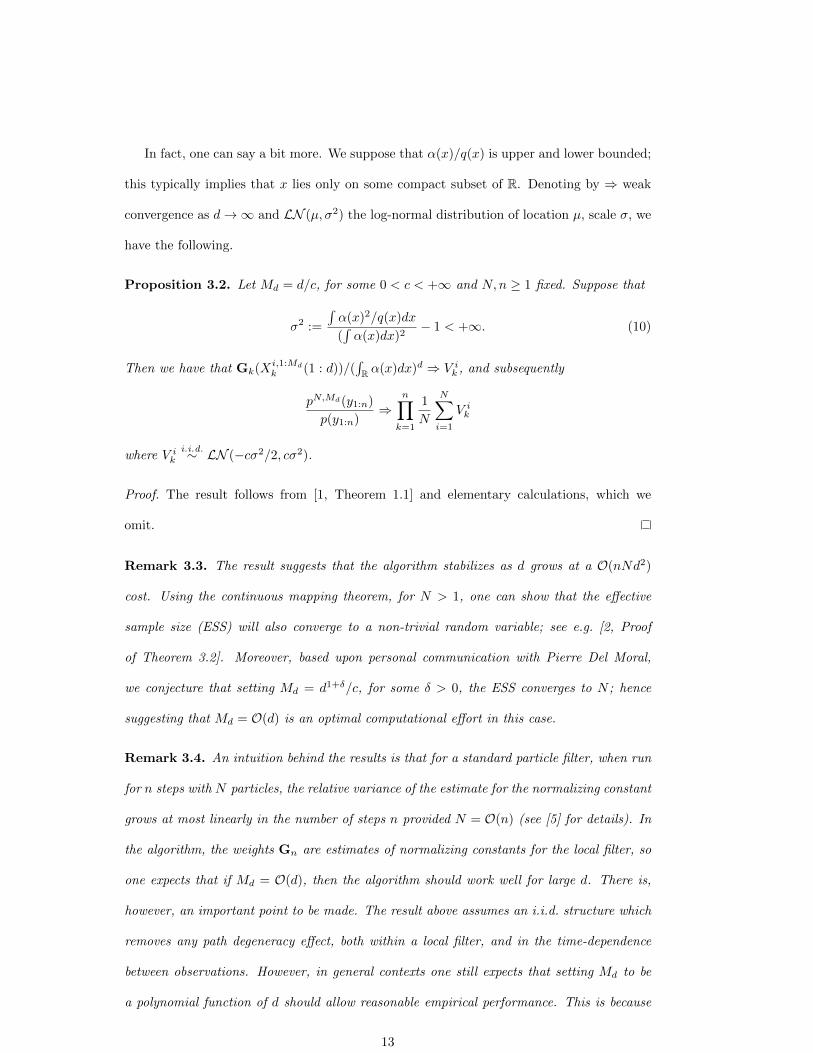
In fact, one can say a bit more. We suppose that α(x)/q(x) is upper and lower bounded;

this typically implies that x lies only on some compact subset of R. Denoting by ⇒ weak

convergence as d→∞ and LN (µ, σ2) the log-normal distribution of location µ, scale σ, we

have the following.

Proposition 3.2. Let Md = d/c, for some 0 < c < +∞ and N,n ≥ 1 fixed. Suppose that

σ2 :=

∫α(x)2/q(x)dx

(∫α(x)dx)2

− 1 < +∞. (10)

Then we have that Gk(Xi,1:Md

k (1 : d))/(∫R α(x)dx)d ⇒ V ik , and subsequently

pN,Md(y1:n)

p(y1:n)⇒

n∏k=1

1

N

N∑i=1

V ik

where V iki.i.d.∼ LN (−cσ2/2, cσ2).

Proof. The result follows from [1, Theorem 1.1] and elementary calculations, which we

omit.

Remark 3.3. The result suggests that the algorithm stabilizes as d grows at a O(nNd2)

cost. Using the continuous mapping theorem, for N > 1, one can show that the effective

sample size (ESS) will also converge to a non-trivial random variable; see e.g. [2, Proof

of Theorem 3.2]. Moreover, based upon personal communication with Pierre Del Moral,

we conjecture that setting Md = d1+δ/c, for some δ > 0, the ESS converges to N ; hence

suggesting that Md = O(d) is an optimal computational effort in this case.

Remark 3.4. An intuition behind the results is that for a standard particle filter, when run

for n steps with N particles, the relative variance of the estimate for the normalizing constant

grows at most linearly in the number of steps n provided N = O(n) (see [5] for details). In

the algorithm, the weights Gn are estimates of normalizing constants for the local filter, so

one expects that if Md = O(d), then the algorithm should work well for large d. There is,

however, an important point to be made. The result above assumes an i.i.d. structure which

removes any path degeneracy effect, both within a local filter, and in the time-dependence

between observations. However, in general contexts one still expects that setting Md to be

a polynomial function of d should allow reasonable empirical performance. This is because

13

the relative variance of the normalizing constant can be controlled in such path dependent

cases, with polynomial cost; see [17] for example.

Remark 3.5. In the case of no global resampling, one would typically use the estimate, for

p(y1:n)

1

N

N∑i=1

n∏k=1

d∏j=1

1

Md

Md∑l=1

α(xik(j))

q(xik(j)).

A weak convergence result also holds in this case.

We now adopt a context of no global resampling and consider the Monte Carlo error of

the following two estimates, for n ≥ 1, l ∈ {1, . . . ,Md} fixed and ϕ ∈ Cb(R),

1

N

N∑i=1

∏nk=1 Gk(xi,1:Md

k (1 : d))∑Nj=1

∏nk=1 Gk(xj,1:Md

k (1 : d))

1

Md

Md∑l=1

ϕ(xi,ln (d))

and

1

N

N∑i=1

∏nk=1 Gk(xi,1:Md

k (1 : d))∑Nj=1

∏nk=1 Gk(xj,1:Md

k (1 : d))ϕ(xi,ln (d)).

We remark that this is the simplest case in terms of analysis, as for example the case of

when global resampling is considered is seemingly more complex. We now give our result;

the technical results for the proof can be found in Appendix C. We set

π(ϕ) =

∫Rα(x)ϕ(x)dx/

∫Rα(x)dx.

For ϕ ∈ Bb(R), we denote ‖ϕ‖∞ := supx∈R |ϕ(x)|. Also Cb(R) are the continuous and

real-valued functions on R.

Theorem 3.2. Let Md = d/c, for some 0 < c < +∞ and n ≥ 1, N > 1 fixed. Then we

have, for any ϕ ∈ Cb(R), 1 ≤ p < +∞

1.

limd→∞

E[∣∣∣ N∑i=1

∏nk=1 Gk(Xi,1:Md

k (1 : d))∑Nj=1

∏nk=1 Gk(Xj,1:Md

k (1 : d))

1

Md

Md∑l=1

ϕ(Xi,ln (d))− π(ϕ)

∣∣∣p]1/p = 0

2. there exists an M(p) < +∞, depending upon p only, such that

limd→∞

E[∣∣∣ N∑i=1

∏nk=1 Gk(Xi,1:Md

k (1 : d))∑Nj=1

∏nk=1 Gk(Xj,1:Md

k (1 : d))ϕ(Xi,l

n (d))− π(ϕ)∣∣∣p]1/p ≤

M(p)‖ϕ‖∞√N

[exp{−cσ2p/2 + cσ2p2/2}+ 1

]1/pwhere σ2 is as in (10).

14

Proof. For Case 1. we have that by Proposition 3.2, and the continuous mapping theorem

that (after scaling the numerator and denominator by (∫α(x)dx)d), for each i∏n

k=1 Gk(Xi,1:Md

k (1 : d))∑Nj=1

∏nk=1 Gk(Xj,1:Md

k (1 : d))⇒

∏nk=1 V

ik∑N

j=1

∏nk=1 V

jk

.

where V ik ∼ LN (−cσ2/2, cσ2), for σ2 as in Proposition 3.2. By standard importance sam-

pling and resampling results (see for instance [15])), we have that

1

Md

Md∑l=1

ϕ(Xi,ln (d))→P π(ϕ).

By Lemma C.1 2., these two terms are asymptotically independent. Thus we have

N∑i=1

∏nk=1 Gk(Xi,1:Md

k (1 : d))∑Nj=1

∏nk=1 Gk(Xj,1:Md

k (1 : d))

1

Md

Md∑l=1

ϕ(Xi,ln (d))⇒ π(ϕ).

The proof of 1. is complete on noting the boundedness of the associated quantities.

For Case 2. by Proposition 3.2, the fact that Xi,ln (d) ⇒ V i ∼ π (see e.g. [15]) and

Lemma C.1 1. we have

N∑i=1

∏nk=1 Gk(Xi,1:Md

k (1 : d))∑Nj=1

∏nk=1 Gk(Xj,1:Md

k (1 : d))ϕ(Xi,l

n (d))⇒N∑i=1

∏nk=1 V

ik∑N

j=1

∏nk=1 V

jk

ϕ(V i)

where the V i are independent of the V ik and have a distribution that has density π. Then,

by the boundedness of the associated quantities we have

limd→∞

E[∣∣∣ N∑i=1

∏nk=1 Gk(Xi,1:Md

k (1 : d))∑Nj=1

∏nk=1 Gk(Xj,1:Md

k (1 : d))ϕ(Xi,l

n (d))− π(ϕ)∣∣∣p]1/p

= E[∣∣∣ N∑i=1

∏nk=1 V

ik∑N

j=1

∏nk=1 V

jk

ϕ(V i)− π(ϕ)∣∣∣p]1/p.

The proof can now be completed by the same calculations as in the proof of [2, Theorem

3.3] and are hence omitted.

Remark 3.6. The main points are, first, that the error in estimation of fixed-dimensional

marginals is independent of d and, second, that averaging over the local particle cloud seems

to help in high dimensions. We repeat that the scaling for Md that stabilises the weights

for the global filter may be over-optimistic for more general models, due to the loss of a

path-degeneracy effect over the observation times in the i.i.d. case.

15

3.3 Stability in High Dimensions for Markov Model

We now consider a more realistic scenario for our analysis in high-dimensions. In order to

read this Section, one will need to consult Appendices B and D; this Section can be skipped

with no loss in continuity.

We consider the interaction of the dimension and the time parameter in the behaviour

of the algorithm. We will now list some assumptions and notations needed to describe the

result.

(A1) For every n ≥ 1 we have

g(xn, yn)f(xn−1, xn) =

d∏j=1

h(yn, xn(j))k(xn(j − 1), xn(j))

where h : Rk → R+, xn(0) = xn−1(d) and for every x ∈ R,∫R k(x, x′)dx′ = 1.

It is noted that even under (A1) a standard particle filter which propagates all d co-ordinates

together may degenerate as d grows. However, as we will remark, the STPF can stabilize

under assumptions, even if N = 1. Our algorithm will use the Markov kernels k(xn(j −

1), xn(j)) as the proposals. Define the semigroup, for p ≥ 1:

qp(xp−1, dxp) = f(xp−1, xp)gp(xp)dxp

where gp(xp) = g(yp, xp). For ϕ ∈ Bb(Rd) define

qp,n(ϕ)(xp) =

∫qp+1(xp, dxp+1)× · · · × qn(xn−1, dxn)ϕ(xn). (11)

(A2) There exists a c <∞, such that for every 1 ≤ p < n and d ≥ 1

supx,y

qp,n(1)(x)

qp,n(1)(y)≤ c.

Note (A2) is fairly standard in the literature (e.g. [7]) and given (A1) it will hold under

some simple assumptions on h and k.

Now, we will consider the global filter with N particles, as standard results in the lit-

erature can provide immediately CLTs and SLLNs for quantities of interest. We will then

investigate the effect of the dimensionality d on the involved terms. Consider the standard

16

estimate for the normalising constant for the global filter

γNn (1) :=

n−1∏p=1

ηNp (Gp)

when ηNp (·) simply denotes Monte-Carlo averages over the N particle systems at time p, see

Appendix B for analytic definitions. From standard particle filtering theory, we have that

ηNp (·) is an unbiased estimator of the corresponding limiting quantity, denoted γn(1), see

e.g. [6, Theorem 7.4.2]. Also, under our assumptions, one has the following CLT as N →∞

(see [6, Proposition 9.4.2])

√N(γNn (1)

γn(1)− 1)⇒ N (0, σ2

n) (12)

where N (0, σ2) is the one dimensional normal distribution with zero mean and variance σ2,

and

σ2n =

1

γn(1)2

n∑p=1

γp(1)2ηp

((Qp,n(1)− ηp(Qp,n(1))

)2).

All bold terms correspond to standard Feynman-Kac quantities and are defined in Appendix

B. We also show in Appendix B that the normalising constant of the global filter coincides

with the one of the original filter of interest, that is

γn(1) ≡ γn(1) =

∫ n−1∏p=1

gp(xp)f(xp−1, xp)dx1:p = p(y1:n−1)

Thus, (12) provides in fact a CLT for the estimate of STPF for p(y1:n−1) proposed in

Theorem 3.1.

We have the following result, whose proof is in Appendix D:

Theorem 3.3. Assume (A1-2). Then there exist a c < ∞ such that for any n, d ≥ 1 and

any Md ≥ cd

σ2n ≤ nc

( d

Md+ 1).

Remark 3.7. Our result establishes that the asymptotic in N variance of the relative value

of the normalizing constant estimate grows at most linearly in n and, if Md = O(d) does

not grow with the dimension. The cost of the algorithm is O(nNd2). The linear growth in

time is a standard result in the literature (see [7]) and one does not expect to do better than

17

this. Note, that a particular model structure is chosen and one expects a higher cost in more

general problems.

Remark 3.8. We expect that to show that the error in estimation of the filter is time uni-

form, under (A1), that one will need to set Md = O(d2). This is because one is performing

estimation on the path of the algorithm; see [7, Theorem 15.2.1 and Corollary 15.2.2]. In-

deed, one can be even more specific; if N = 1, then one can show that, under (A1-2) that the

Lp-error associated to the estimate of the filter (applied to a bounded test function in Rd) at

time n is upper-bounded by c‖ϕ‖∞d/√Md (via [7, Theorem 15.2.1, Corollary 15.2.2]) with

c independent of d and n. Thus setting Md = O(d2), the upper-bound depends on d only

through ‖ϕ‖∞.

4 Numerical Results

4.1 Example 1

We consider the following simple model. Let Xn ∈ Rd be such that we have X0 = 0d (the

d-dimensional vector of zeros) and

Xn(j) =

j−1∑i=1

βd−j+i+1Xn(i) +

d∑i=j

βi−j+1Xn−1(i) + εn

where εni.i.d.∼ N (0, σ2

x) and β1:d are some known static parameters. For the observations,

we set

Yn = Xn + ξn

where ξn(j)i.i.d.∼ N (0, σ2

x), j ∈ {1, . . . , d}. It is easily shown that this linear Gaussian model

has the structure (1).

We consider the standard particle filter and the STPF. The data are simulated from the

model with σ2x = σ2

y = 1 and n = 1000 d-dimensional observations. These parameters are

also used within the filters. Both filters use the model transitions as the proposal and the

likelihood function as the potential. For STPF we use N = 1000 and Md = 100, and for the

particle filter algorithm we use NMd particles. Adaptive resampling is used in all situations

18

(with appropriate adjustment to the formula of calculating the weights for each of the N

particles, as well as the estimates). Some results for d ∈ {10, 100, 1000} are presented in

Figures 1 to 3.

Standard Particle Filter Space−Time Particle Filter

−5

0

5

10

15

20

−2.5

0.0

2.5

5.0

7.5

10.0

0.0

2.5

5.0

7.5

10.0

12.5

d = 10

d = 100

d = 1000

0 250 500 750 1000 0 250 500 750 1000Time

Mea

n of

Est

imat

ors

for

X(1

)

Observation Average of Estimates

Figure 1: Mean of estimators of Xn(1) for Example 4.1 across 100 runs.

The averages of estimators per time step (for the posterior mean of the first co-ordinate

Xn(1) given all date up to time n) across 100 separate algorithmic runs are illustrated

in Figure 1. For STPF, the estimator corresponds to the double average over Md, N as

shown in Section 2. The figure shows that the particle filter collapses when the dimension

become moderate or large. It is unable to provide meaningful estimates when d = 1000 (as

the estimates completely lose track of the observations). In contrast, the STPF performs

19

d = 10

d = 100

d = 1000

0.00

0.25

0.50

0.75

1.00

0.0

0.2

0.4

0.6

0.8

0.00

0.01

0.02

0.03

0.04

0 250 500 750 1000Time

ES

S (

scal

ed b

y th

e nu

mbe

r of

par

ticle

s)

Standard Particle Filter Space−Time Particle Filter

Figure 2: Effective Sample Size plots for Example 4.1 from a single run.

reasonably well in all three cases. In Figure 2 we can observe the ESS (scaled by the

number of particles) for each time step of the two algorithms. The standard filter struggles

significantly even in the case d = 10 and it collapses when d = 1000. The performance of

the new algorithm is deteriorating (but not collapsing) when the dimension increases. This

is inevitably due to the path degeneracy effect that we have mentioned. These conclusions

are further supported in Figure 3 where the variance per time step for the estimators of the

posterior mean of the first co-ordinate Xn(1) (given the data up to time n) across 100 runs

is displayed.

20

d = 10

d = 100

d = 1000

0.001

0.100

0.001

0.100

0.001

0.100

0 250 500 750 1000Time

Var

ianc

e of

Est

imat

ors

for

X(1

)

Standard Particle Filter Space−Time Particle Filter

Figure 3: Variance (on logarithm scale) for estimators of Xn(1) for Example 4.1 across 100

runs.

4.2 Example 2

4.2.1 Model and Simulation Settings

We consider the following model on a two-dimensional graph, which follows that described in

[14]. Let the components of state Xn be indexed by vertices v ∈ V , where V = {1, . . . , d}2.

The dimension of the model is thus d2. The distance between two vertices, v = (a, b) and

u = (c, d), is calculated in the usual Euclidean sense, D(v, u) =√

(a− c)2 + (b− d)2. At

21

time n, Xn(v) follows a mixture distribution,

f(xn−1, xn(v)) =∑

u∈N(v)

wu(v)fu(xn−1(u), xn(v))

where N(v) = {u : D(v, u) ≤ r} for r ≥ 1 is the neighborhood of vertex v. For observations,

Yn = Xn + ξn

where ξn(v), v ∈ V are i.i.d. t-distributed random variables with degree of freedom ν.

In this example, we use a Gaussian mixture with component mean Xn−1(u) and unity

variance. The weights are set to be wu(v) ∝ 1/(D(v, u)+δ) and∑u∈N(v) wu(v) = 1. In other

words, when δ → 0, each vertex evolves as a Gaussian random walk itself. We simulated

data from model r = 1, δ = 1, ν = 10 and d = 32. It results in a 1024 dimensional model.

These parameters are also used in the filters.

We will compare the standard particle filter, the STPF, the marginal STPF algorithm

(as described in Section 2.4) and the block particle filter (BPF) in [14] (notice that the block

particle filter is characterised by space varying bias, by construction). The simulations for

the STPF versions are done with N = Md = 100. The number of particles for the standard

particle filter and BPF are NMd. For the marginal algorithm, we also simulated with N = 1

and Md = 1000. The block size of BPF is set to be b2, b ∈ {1, . . . , d}, and it is partitioned

such that each block is itself a square. The MCMC moves of the marginal algorithm are

simple Gaussian random walks with standard deviation (the scale) being 0.5. The optimal

block size in [14] is about b = 7 for ten thousand particles and a two-dimensional graph.

Thus, we considered the cases b = 4 and 8, the two nearest integers such that d is divisible

by b.

4.2.2 Results

A single run takes around 2 minutes for the standard particle filter and the block filter on an

Intel Xeon W3550 CPU, with four cores and eight threads. It takes around 10 minutes for

the STPF. It takes about 40 minutes for the marginal algorithm with N = 1 and Md = 1000,

and about 7 hours for N = Md = 100.

22

The standard particle filter performs poorly and cannot provide adequate estimates

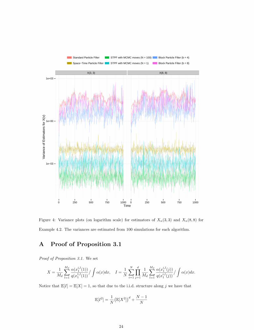
(similar to the d = 1000 case in the previous example). In Figure 4, we observe the variance

per time step of the estimators for two vertices, across 30 runs. The first vertex, Xn(3, 3) is

not on the boundary of either block size and the second, Xn(8, 8) is on the boundary of both

block sizes. In either case, the STPF significantly outperforms the block filter, albeit under

slightly longer run times. The STPF does not collapse in high-dimensions, but perhaps

does not have excellent performance. The marginal STPF performs very well, but the

computational time is substantially higher than all of the other algorithms. However, with

N = 1 and Md = O(d), the marginal STPF provides a good balance between performance

and computational cost in challenging situations where the path degeneracy may hinder

successful application of the new algorithm.

The block filter variance for Xn(8, 8) (boundary vertex) is about twice that of Xn(3, 3)

while the new algorithm performs equally well for both cases.

5 Summary

In this article we have considered a novel class of particle algorithms for high-dimensional

filtering problems and investigated both theoretical and practical aspects of the algorithm.

We believe the article opens new directions in an important and challenging Monte-Carlo

problem, and several aspects of the method remain to be investigated in future research.

There are indeed several possible extensions to the work in this article. In particular, an

analysis of the algorithm when the structure of the state-space model is more complex than

the structures considered in this article. We expect that in such scenarios, that the cost

of the algorithm should increase, but only by a polynomial factor in d. In addition, the

interaction of dimension and time behaviour is of particular interest.

Acknowledgements

Ajay Jasra and Yan Zhou were supported by ACRF tier 2 grant R-155-000-143-112. We

thank Pierre Del Moral for many useful conversations on this work.

23

X(3, 3) X(8, 8)

1e−03

1e+00

1e+03

0 250 500 750 1000 0 250 500 750 1000Time

Var

ianc

e of

Est

imat

ors

for

X(v

)

Standard Particle Filter

Space−Time Particle Filter

STPF with MCMC moves (N = 100)

STPF with MCMC moves (N = 1)

Block Particle Filter (b = 4)

Block Particle Filter (b = 8)

Figure 4: Variance plots (on logarithm scale) for estimators of Xn(3, 3) and Xn(8, 8) for

Example 4.2. The variances are estimated from 100 simulations for each algorithm.

A Proof of Proposition 3.1

Proof of Proposition 3.1. We set

X =1

Md

Md∑l=1

α(xi,l1 (1))

q(x1,l1 (1))

/∫α(x)dx, I =

1

N

N∑i=1

d∏j=1

1

Md

Md∑l=1

α(xi,l1 (j))

q(xi,l1 (j))

/∫α(x)dx.

Notice that E[I] = E[X] = 1, so that due to the i.i.d. structure along j we have that

E[I2] =1

N

(E[X2]

)d+N − 1

N

24

Also, due to the i.i.d. structure along j, l we have

E[X2] =1

Md

∫a2(x)/q(x)dx( ∫a(x)dx

)2 +Md − 1

Md.

Finally, we have that, due to i.i.d. structure along n,

E[(pN,Md(y1:n)

p(y1:n)− 1)2]

= E[( pN,Md(y1:n)( ∫

α(x)dx)nd)2]

− 1

= (E[I2])n − 1.

A synthesis of the above three equations gives the required result.

B Proof of Theorem 3.1

B.1 Further Notation

In order to prove Theorem 3.1, we will first introduce another round of notations. Let

(En,En)n≥0 be a sequence of measurable spaces endowed with a countably generated σ-field

En. The set Bb(En) denotes the class of bounded En/B(R)-measurable functions on En where

B(R) is the Borel σ-algebra on R. We will consider non-negative operators K : En−1×En →

R+ such that for each x ∈ En−1 the mapping A 7→ K(x,A) is a finite non-negative measure

on En and for each A ∈ En the function x 7→ K(x,A) is En−1/B(R)-measurable; the kernel

K is Markovian if K(x, dy) is a probability measure for every x ∈ En−1. For a finite measure

µ on (En−1,En−1) and Borel test function f ∈ Bb(En) we define

µK : A 7→∫K(x,A)µ(dx); Kf : x 7→

∫f(y)K(x, dy).

B.2 Feynman-Kac Model on Enlarged Space

We will define a Feynman-Kac model on an appropriate enlarged space. That is, one Markov

transition on the enlarged space will correspond to one observation time and will collect all

d space-steps of the local filter for this time-step. Some care is needed with the notation, as

we need to keep track of the development of the co-ordinates at time n, together with the

states at time n− 1 as the latter are involved in the proposal.

25

Time-Step 1: Consider observation time 1 of the algorithm. We define a sequence

of random variables Zl1,j with j ∈ {1, . . . , d + 1}, 1 ≤ l ≤ Md, such that Zl1,j ∈ Rj , for

j ∈ {1, . . . , d}, and Zl1,d+1 ∈ Rd. For j ∈ {1, . . . , d} we will write the co-ordinates of Zl1,j as

(Zl1,j(1), . . . , Zl1,j(j)), with the obvious extension for the case j = d+ 1. As x0 is fixed, we

will drop it from our notations, as will become clear below. Also, for simplicity we simply

write q(·) instead of the analytical q1,j(·) as the subscripts are implied by those of Z1,j . We

follow this convention throughout Appendix B. We define the following sequence of Markov

kernels corresponding to the proposal for the co-ordinates at the first time step:

M1,1(dz1,1) = q(z1,1)dz1,1, j = 1,

M1,j(z1,j−1, dz1,j) = q(z1,j(j)|z1,j−1)dz1,j(j) δ{z1,j−1}(dz1,j(1 : j − 1)), j ∈ {1, . . . , d},

M1,j(z1,j−1, dz1,j) = δ{z1,j−1}(dz1,j), j = d+ 1.

Next, we will take under consideration the weights and the resampling. For j ∈ {1, . . . , d}

and a probability measure µ on Rj define

Φ1,j+1(µ)(dz) =

∫Rj µ(dz′)G1,j(z

′)M1,j+1(z′, dz)∫Rj µ(dz′)G1,j(z′)

.

For the local particle filter in observation time 1, write the un-weighted empirical measure

ηMd1,j (dz) =

1

Md

Md∑l=1

δzl1,j (dz), j ∈ {1, . . . , d}.

We also consider all random variables involved at time-step 1 and set

z1 = (z1:Md1,1 , . . . , z1:Md

1,d+1).

The joint law of the samples required by the local filter is

η1(dz1) =(Md∏l=1

M1,1(dzl1,1))( d+1∏

j=2

Md∏l=1

Φ1,j(ηMd1,j−1)(dzl1,j)

)). (13)

Notice, that in the notation we have established herein, the potential G1 defined in the

main text can now equivalently be expressed as

G1(z1) =

d∏j=1

ηMd1,j (G1,j). (14)

We also set zl1,d+1(1) = zl1,d+1.

26

Time-Step n ≥ 2: At subsequent observation times, n ≥ 2, we again work with variables

denoted Zln,j , with j ∈ {1, . . . , d+1}, but this time we have to keep track of the corresponding

paths at time n − 1, thus we will use the notation Zln,j = (Zl,+n,j , Zl,−n,j ), with Zl,+n,j ∈ Rj ,

Zl,−n,j ∈ Rd, with the latter component referring to the ‘tail’ at time n− 1 of the path found

at Z+n,j at time n and space position j. So, we have Zln,j ∈ Rj+d, j ∈ {1, . . . , d} and

Zln,d+1 ∈ R2d. We define the following sequence of kernels:

Mn,1(z+n−1,d+1, dzn,1) = q(z+

n,1|z+n−1,d+1)dz+

n,1 δ{z+n−1,d+1}(dz−n,1), j = 1,

Mn,j(zn,j−1, dzn,j) = q(z+n,j(j)|zn,j−1)dz+

n,j(j) δ{z+n,j−1}(dz+

n,j(1 : j − 1))

· δ{z−n,j−1}(dz−n,j), j ∈ {1, . . . , d},

Mn,d+1(zn,d, dzn,d+1) = δ{zn,d}(dzn,d+1), j = d+ 1.

For j ∈ {2, . . . , d} and a probability measure µ on Rj+d define the measure on Rmin{j+1,d}+d

Φn,j+1(µ)(dz) =

∫µ(dz′)Gn,j(z

′)Mn,j+1(z′, dz)∫µ(dz′)Gn,j(z′)

.

For the local particle filter at space-step j, we write the empirical measure

ηMdn,j (dz) =

1

Md

Md∑l=1

δzln,j(dz), j ∈ {1, . . . , d}.

Set zn = (z1:Mdn,1 , . . . , z1:Md

n,d+1). The transition law of all involved samples in the local particle

filter is

Mn(zn−1, dzn) =(Md∏l=1

Mn,1(zl,+n−1,d+1, dzln,1))( d+1∏

j=2

Md∏l=1

Φn,j(ηMdn,j−1)(dzln,j)

)). (15)

Then, we will work with the potential

Gn(zn) =

d∏j=1

ηMdn,j (Gn,j). (16)

The algorithm described in Section 2 corresponds to a standard particle filter approxi-

mation (with N particles) of a Feynman-Kac model specified by the initial distribution (13),

the Markovian transitions (15) and the potentials in (14), (16). Thus, for the Monte-Carlo

algorithm with N particles, set ηNn for the N -empirical measure of z1:Nn and set, for µ a

probability measure, n ≥ 2

Φn(µ)(dz) =

∫µ(dz′)Gn−1(z′)Mn(z′, dz)∫

µ(dz′)Gn−1(z′).

27

Then our global filter samples from the path measure, up-to observation time n

( N∏i=1

η1(dzi1))( n∏

k=2

N∏i=1

Φk(ηNk−1)(dzik))

not including resampling at observation time n. We use the standard definition of the

normalising constant for any n ≥ 1

γn(ϕ) =

∫η1(dz1)

n∏p=2

Gp−1(zp−1)Mp(zp−1, dzp)ϕ(zn) (17)

and set

ηn(ϕ) =γn(ϕ)

γn(1), (18)

thus ηn corresponds to the predictive distribution at time n for the global filter. Notice,

that from (17), we can equivalently write for the unnormalised measure

γn(ϕ) = η1(G1M2(G2M3 · · · (Gn−1Mn(ϕ)))). (19)

B.3 Calculation of Quantities for Global Filter

We consider functions of the particular form

φ(zp) =1

Md

Md∑l=1

φ(zl,+p,d+1), φ ∈ Bb(Rd).

For functions of the above type, we write φ ∈ Ap. We will illustrate that upon application

on this family, several Feynman-Kac quantities of the global model (with signal dynamics

η1,M2,. . . , and potentials G1,G2 . . . ) coincide with those of the original model of inter-

est (with signal dynamics f1, f2, . . . and potentials g1, g2, . . .). In particular we calculate

Mp(Gpφ) as, from (19), it is the building block for other expressions. Notice we can write

Mp(Gpφ) =

∫Mp(zp−1, dzp)Gp(zp)

1

Md

Md∑l=1

φ(zl,+p,d+1) =

∫ (Md∏l=1

Mp,1(zl,+p−1,d+1, dzlp,1))( d+1∏

j=2

Md∏l=1

Φp,j(ηMdp,j−1)(dzlp,j)

)) d∏j=1

ηMdp,j (Gp,j) · ηMd

p,d+1(φ).

So, the integral concerns now the local particle filter with weights Gp,j and Markov kernels

Mq,j . In particular, the integral corresponds to the expected value of the particle approxi-

mation of the standard Feynamn-Kac unnormalised estimator with standard unbiasedness

28

properties [6, Theorem 7.4.2]. That is, the integral is equal to (here, for each l, the process

zlp,1, zlp,2, . . . , z

lp,d+1 is a Markov chain evolving viaMp,1(zl,+p−1,d+1, dz

lp,1),Mp,2(zlp,1, dz

lp,2), . . . ,

Mp,d+1(zlp,d, dzlp,d+1) respectively)

1

Md

Md∑l=1

E[φ(zlp,d+1)Gp,d(z

lp,d) · · ·Gp,2(zlp,2)Gp,1(zlp,1)|zl,+p−1,d+1

].

From the analytical definition of the kernels and the weights, this latter quantity is easily

seen to be equal to

1

Md

Md∑l=1

∫φ(z)

d∏j=1

αp,j(yp, zl,+p−1,d+1, z(1 : j))dz(1 : j) =

1

Md

Md∑l=1

∫φ(z)fp(z

l,+p−1,d+1, dz)gp(z, yp)dz

= ηMd

p−1,d+1(fp(gpφ)).

So, we have obtained that

Mp(Gpφ) = ηMd

p−1,d+1(fp(gpφ)) ∈ Ap−1. (20)

Thus, applying the above result recursively, we obtain from (19) that

γn(Gnφ) =

∫ n∏p=1

fp(xp−1, dxp)gp(xp, yp)φ(xp). (21)

Using the standard Feynman-Kac notation, this latter integral can be denoted as γn(gnφ)

for the unnormalised measure γn. Thus, for instance, for the normalising constants, we have

that

γn(Gn) = γn(gn) ≡ p(y1:n). (22)

B.4 Proof

We have established that the algorithm is a standard particle filter approximation of a

Feynman-Kac formula on an extended space. Thus, standard results, e.g. in [6], will give

consistency for Monte-Carlo estimates on the enlarged state-space. In only remains to

show that indeed the quantities in the statement of Theorem 3.1 correspond to Monte-

Carlo averages of the global filter in the enlarged space. We look directly at the last two

quantities in the statement of the Theorem, as the derivation for the first two ones is similar

29

and simpler. For the first we set

ϕ(zn) =1

Md

Md∑l=1

ϕ(zl,+n,d+1) ∈ An,

and we immediately have that (denoting by zin the resampled islands, under the weights

Gn(zin))

1

N

N∑i=1

ϕ(zin)→P

∫ηn(dzn)Gn(zn)ϕ(zn)∫ηn(dzn)Gn(zn)

=γn(Gnϕ)

γn(Gn).

Notice now that the quantity on the left is precisely the double average in the statement of

the Theorem and the quantity on the right, from (21), is equal to γn(gnϕ)/γn(gn) = πn(ϕ).

For the last statement in the Theorem, the quantity on the left is γNn (Gn) which, from

standard particle filter theory converges in probability to γn(Gn) = γn(gn) = p(y1:n).

C Monte Carlo Averages

Below let V ∈ R be a random variable with probability density α(x)/∫R α(x)dx. Recall that

Xi,ln (d) is particle i, local particle l at observation time n, dimension d and it has just been

locally resampled using the weights Gn,d(xi,ln (d)). Recall that there is no global resampling.

Throughout Md = d/c (assumed to be integer, for notational convenience).

Lemma C.1. Let n ≥ 1, i ∈ {1, . . . , N}, l ∈ {1, . . . ,Md} be fixed and ϕ ∈ Bb(R). Then

1. Gn(xi,1:Mdn (1 : d))/(

∫α(x)dx)d and ϕ(xi,ln (d))

2. Gn(xi,1:Mdn (1 : d))(

∫α(x)dx)d and 1

Md

∑Md

l=1 ϕ(xi,ln (d))

are asymptotically independent as d→∞.

Proof. We first consider statement 1. Set r =√−1 and consider the standardised quantity

Gn(xi,1:Mdn (1 : d)) = Gn(xi,1:Md

n (1 : d))/(∫α(x)dx)d, then we have that for (t1, t2) fixed,

E[

exp{rt1Gn(Xi,1:Md

n (1 : d)) + rt2ϕ(Xi,ln (d))

}]=

E

[exp

{rt1Gn(Xi,1:Md

n (1 : d))}∑Md

l=1Gn,d(Xi,ln (d))ert2ϕ(Xi,l

n (d))∑Md

l=1Gn,d(Xi,ln (d))

].

By standard SLLN, we have that∑Md

l=1Gn,d(Xi,ln (d))ert2ϕ(Xi,l

n (d))∑Md

l=1Gn,d(Xi,ln (d))

→P

∫R α(x)ert2ϕ(x)dx∫

R α(x)dx.

30

Also, Proposition 3.2 implies that

exp{rt1Gn(Xi,1:Mdn (1 : d))} ⇒ exp{rt1V in}

where V in ∼ LN (−cσ2/2, cσ2) for σ2 defined therein. Hence, from Slutsky’s lemmas we have

exp{rt1Gn(Xi,1:Mdn (1 : d))}

∑Md

l=1Gn,d(Xi,ln (d))ert2ϕ(Xi,l

n (d))∑Md

l=1Gn,d(Xi,ln (d))

⇒ exp{rt1V in}∫R α(x)ert2ϕ(x)dx∫

R α(x)dx.

The proof of 1. is concluded on noting the boundedness of the functions.

For the proof of 2. we have

E[ert1Gn(X

i,1:Mdn (1:d))+rt2

1Md

∑Mdl=1 ϕ(Xi,l

n (d))]

=

E[ert1Gn(X

i,1:Mdn (1:d))

[ert2

1Md

∑Mdl=1 ϕ(Xi,l

n (d)) − ert2π(ϕ)]]

+ ert2π(ϕ)E[ert1Gn(X

i,1:Mdn (1:d))

]=: Ad +Bd (23)

where we have used the short-hand π(ϕ) =∫R α(x)ϕ(x)dx/

∫R α(x)dx. From standard

importance sampling and resampling results (see e.g. [15]), we have that

1

Md

Md∑l=1

ϕ(Xi,ln (d))→P

∫R α(x)ϕ(x)dx∫

R α(x)dx.

So, returning to (23), we have obtained that Ad →P 0, thus

limd→∞

E[ert1Gn(X

i,1:Mdn (1:d))+rt2

1Md

∑Mdl=1 ϕ(Xi,l

n (d))]

= exp{rt2π(ϕ)}E[exp{rt1V in}]

which concludes the proof of 2..

D Proof of Theorem 3.3

Recall the notation for the global filter from Appendix B. We define the semi-group

Qp+1(zp, dzp+1) = Gp(zp)Mp+1(zp, dzp+1)

and we also set

Qp,n(ϕ) =

∫Qp+1(zp, dzp+1)× · · · ×Qn(zn−1, dzn)ϕ(zn). (24)

Recall from the main result in (20) in Appendix B, connecting the global with the local

filter, that Mp(Gp) = ηMd

p−1,d+1(fp(gp)), and upon an iterative application of this result

Qp,n(1) = Gp(zp)ηMd

p,d+1(qp+1,n−1(1)). (25)

31

We also have that γn(1) = γn(1) = γp(gpqp+1,n−1(1)) = πp(qp+1,n−1(1))γp(gp) and, finally,

that γp(gp) = πp−1(fp(gp))γp(1). Using all these expressions, simple calculations will give

σ2n =

n∑p=1

γp(1)2

γn(1)2ηp

((Qp,n(1)− ηp(Qp,n(1))

)2)

=

n∑p=1

ηp

(( Gp(zp)

Mp(Gp)Ap − 1

)2)

(26)

where we have defined

Ap =ηMdp (qp+1,n−1(1))

πp(qp+1,n−1(1))·ηMdp−1(fp(gp))

πp−1(fp(gp)).

The main thing to notice now, is that Gp(zp)/Mp(Gp) corresponds to the standard estimate

of the normalising constant for the p-th local filter divided with its expected value, and we

can use standard results from the literature to control its second moment. Indeed, by

Assumptions (A1-2) and [7, Theorem 16.4.1] (see Remark D.1), there exists c < ∞ (which

does not depend on p or zp) such that for any d ≥ 1 and any Md ≥ cd

Mp

(( Gp(zp)

Mp(Gp)− 1)2)≤ c(2 + e)d

Md,

where the upper-bound only depends on d via the term d/Md. Notice also that fp(gp) ≡

qp−1,p(1), so by (A2) and Jensen’s inequality (so that Md/∑Md

i=1 xi ≤∑Md

i=11xi/Md for

positive xi), we have

0 ≤ Ap ≤ c4.

Thus, returning in (26), and using the last two equations, we get, starting with the C2-

inequality

ηp

(( Gp(zp)

Mp(Gp)Ap − 1

)2)≤ 2ηp

(( Gp(zp)

Mp(Gp)− 1)2

c8)

+ 2ηp((Ap − 1)2

)= 2c8γp−1

(Gp−1Mp

(Gp(zp)

Mp(Gp)− 1)2)/γp(1) + 2ηp

((Ap − 1)2

)≤ 2c8c(2 + e)d

Md+ 2c8.

From here, one can easily complete the proof and hence we conclude.

Remark D.1. In the proof of Theorem 3.3 we have used [7, Theorem 16.4.1]. This is a

result on the relative variance of the particle estimate of the normalizing constant, and as

32

stated in [7] does not include a function, i.e. an estimate of the form∏dj=1 η

Mdp,j (Gp,j)η

Mdp,j (ϕ)

for some ϕ ∈ Bb(Rd). Based on personal communication with Pierre Del Moral, [7, Theorem

16.4.1] can be extended to include a function, by modification of the potential functions and

the use of the final formula in [7, pp. 484].

References

[1] Berard, J., Del Moral, P., & Doucet, A. (2015). A log-normal central limit theorem

for particle approximations of normalizing constants. Elec. J. Probab. (to appear).

[2] Beskos, A., Crisan, D. & Jasra, A. (2014). On the stability of sequential Monte Carlo

methods in high dimensions. Ann. Appl. Probab., 24, 1396-1445.

[3] Beskos, A., Crisan, D., Jasra, A. & Whiteley, N. P. (2014). Error bounds and

normalizing constants for sequential Monte Carlo samplers in high-dimensions. Adv.

Appl. Probab., 46, 279–306.

[4] Bickel, P., Li, B. & Bengtsson, T. (2008). Sharp failure rates for the bootstrap

particle filter in high dimensions. In Pushing the Limits of Contemporary Statistics, B.

Clarke & S. Ghosal, Eds, 318–329, IMS.

[5] Cerou, F., Del Moral, P. & Guyader, A. (2011). A non-asymptotic variance theorem

for un-normalized Feynman-Kac particle models. Ann. Inst. Henri Poincare, 47, 629–

649.

[6] Del Moral, P. (2004). Feynman-Kac Formulae: Genealogical and Interacting Particle

Systems with Applications. Springer: New York.

[7] Del Moral, P. (2013). Mean Field Simulation for Monte Carlo Integration Chapman

& Hall: London.

[8] Del Moral, P., Doucet, A. & Jasra, A. (2006). Sequential Monte Carlo samplers.

J. R. Statist. Soc. B, 68, 411–436.

33

[9] Del Moral, P., Doucet, A. & Jasra, A. (2012). On adaptive resampling procedures

for sequential Monte Carlo methods. Bernoulli, 18, 252-278.

[10] Doucet, A. & Johansen, A. (2011). A tutorial on particle filtering and smoothing:

Fifteen years later. In Handbook of Nonlinear Filtering (eds. D. Crisan et B. Rozovsky),

Oxford University Press: Oxford.

[11] Johansen, A. M., Whiteley, N. & Doucet, A. (2012). Exact approximation of

Rao-Blackwellised particle filters. In Proc. 16th IFAC Symp. Systems Ident.

[12] Kantas, N., Beskos, A., & Jasra, A. (2014). Sequential Monte Carlo for inverse

problems: a case study for the Navier Stokes equation. SIAM/ASA JUQ, 2, 464–489.

[13] Poyiadjis, G., Doucet, A & Singh, S. S. (2011). Particle approximations of the score

and observed information matrix in state space models with application to parameter

estimation. Biometrika, 98, 65–80.

[14] Rebeschini, P. & Van Handel, R. (2015). Can local particle filters beat the curse of

dimensionality? Ann. Appl. Probab. (to appear).

[15] Rubin, D. (1988). Using the SIR algorithm to simulate posterior distributions. Bayesian

statistics 3, 395–402. .

[16] Verge, C., Dubarry, C., Del Moral, P. & Moulines, E. (2014). On parallel imple-

mentation of Sequential Monte Carlo methods: the island particle model. Stat. Comp.

(to appear).

[17] Wang, J., Jasra, A., & De Iorio, M. (2014). Computational methods for a class of

network models. J. Comp. Biol., 21, 141-161.

34