64

A State Machine Design for High Level Control of an
Autonomous Wheel Loader
Niclas Evestedt
January 25, 2011

Abstract
This thesis is done as a part of the Autonomous machine project at Volvo Construction Equipment in
Eskilstuna. The goal is to develop a high level control structure capable of performing one complete
load and haul cycle at NCCs asphalt plant in Kjula at 30% productivity. A state machine which
serially executes the stages necessary to complete the whole cycle is designed and integrated into the
subsystems that are already developed. Due to weather conditions the system were never evaluated
at the asphalt plant, instead a simulated working environment were constructed and the system
reached 37.8% productivity compared to a novice driver at this site. To overcome the issues found
during the development a sketch of a new system, redesigned from scratch, is also included in this
report.

Acknowledgements
I would like to thank Robin Lilja for his nerdy humour that has created many laughs on days were
we saw no hope. I would also like to thank Jonatan Blom who have withstood all my complaints
and questions about the wheel loader during the work and of course Torbjörn Martinsson for his
courage when letting two young students play with his expensive wheel loader!

Contents
1 Introduction 2
1.1 Background . . . . . . . . . . . . . . . . . . . . . . . . . . . . . . . . . . . . . . . . . 2
1.2 Problem description . . . . . . . . . . . . . . . . . . . . . . . . . . . . . . . . . . . . 3
1.2.1 Requirements . . . . . . . . . . . . . . . . . . . . . . . . . . . . . . . . . . . . 3
1.3 Thesis outline . . . . . . . . . . . . . . . . . . . . . . . . . . . . . . . . . . . . . . . . 3
2 Current system 4
2.1 Hardware design . . . . . . . . . . . . . . . . . . . . . . . . . . . . . . . . . . . . . . 5
2.1.1 Sensors . . . . . . . . . . . . . . . . . . . . . . . . . . . . . . . . . . . . . . . 5
2.2 Software design . . . . . . . . . . . . . . . . . . . . . . . . . . . . . . . . . . . . . . . 6
2.2.1 PIP8 . . . . . . . . . . . . . . . . . . . . . . . . . . . . . . . . . . . . . . . . . 7
2.2.2 PC . . . . . . . . . . . . . . . . . . . . . . . . . . . . . . . . . . . . . . . . . . 8
2.3 Limitations and drawbacks . . . . . . . . . . . . . . . . . . . . . . . . . . . . . . . . 10
2.3.1 Sensors . . . . . . . . . . . . . . . . . . . . . . . . . . . . . . . . . . . . . . . 10
2.3.2 Software . . . . . . . . . . . . . . . . . . . . . . . . . . . . . . . . . . . . . . . 10
3 Related work 12
3.1 Introduction . . . . . . . . . . . . . . . . . . . . . . . . . . . . . . . . . . . . . . . . . 12
3.2 DARPA Grand Challenge . . . . . . . . . . . . . . . . . . . . . . . . . . . . . . . . . 13
3.3 Stanley . . . . . . . . . . . . . . . . . . . . . . . . . . . . . . . . . . . . . . . . . . . 13
3.3.1 Hardware . . . . . . . . . . . . . . . . . . . . . . . . . . . . . . . . . . . . . . 13
3.3.2 Software . . . . . . . . . . . . . . . . . . . . . . . . . . . . . . . . . . . . . . . 14
3.3.3 Conclusions . . . . . . . . . . . . . . . . . . . . . . . . . . . . . . . . . . . . . 15
3

Contents
4 Design 17
4.1 The NCC cycle . . . . . . . . . . . . . . . . . . . . . . . . . . . . . . . . . . . . . . . 17
4.1.1 Translation to pile . . . . . . . . . . . . . . . . . . . . . . . . . . . . . . . . . 18
4.1.2 Fill bucket . . . . . . . . . . . . . . . . . . . . . . . . . . . . . . . . . . . . . 18
4.1.3 Translation to pocket . . . . . . . . . . . . . . . . . . . . . . . . . . . . . . . 18
4.1.4 Unload bucket . . . . . . . . . . . . . . . . . . . . . . . . . . . . . . . . . . . 19
4.2 Design problems . . . . . . . . . . . . . . . . . . . . . . . . . . . . . . . . . . . . . . 19
4.3 State machine . . . . . . . . . . . . . . . . . . . . . . . . . . . . . . . . . . . . . . . . 20
4.3.1 Translation to pile . . . . . . . . . . . . . . . . . . . . . . . . . . . . . . . . . 20
4.3.2 Fill bucket . . . . . . . . . . . . . . . . . . . . . . . . . . . . . . . . . . . . . 21
4.3.3 Translation to pocket . . . . . . . . . . . . . . . . . . . . . . . . . . . . . . . 22
4.3.4 Unload state . . . . . . . . . . . . . . . . . . . . . . . . . . . . . . . . . . . . 23
4.4 Sitecontroller . . . . . . . . . . . . . . . . . . . . . . . . . . . . . . . . . . . . . . . . 24
4.5 System design . . . . . . . . . . . . . . . . . . . . . . . . . . . . . . . . . . . . . . . . 24
4.5.1 Overview . . . . . . . . . . . . . . . . . . . . . . . . . . . . . . . . . . . . . . 25
4.5.2 Vision state machine . . . . . . . . . . . . . . . . . . . . . . . . . . . . . . . . 25
4.5.3 Navigation state machine . . . . . . . . . . . . . . . . . . . . . . . . . . . . . 26
4.5.4 Main state machine . . . . . . . . . . . . . . . . . . . . . . . . . . . . . . . . 27
4.5.5 Top level . . . . . . . . . . . . . . . . . . . . . . . . . . . . . . . . . . . . . . 27
4.5.6 NCC cycle . . . . . . . . . . . . . . . . . . . . . . . . . . . . . . . . . . . . . . 28
5 Implementation 32
5.1 State machine . . . . . . . . . . . . . . . . . . . . . . . . . . . . . . . . . . . . . . . . 32
5.1.1 .NET State Machine Toolkit . . . . . . . . . . . . . . . . . . . . . . . . . . . 32
5.1.2 State machine controller . . . . . . . . . . . . . . . . . . . . . . . . . . . . . . 33
5.2 Supplementary functions . . . . . . . . . . . . . . . . . . . . . . . . . . . . . . . . . . 34
5.2.1 Path planning . . . . . . . . . . . . . . . . . . . . . . . . . . . . . . . . . . . . 34
5.2.2 Weight estimation . . . . . . . . . . . . . . . . . . . . . . . . . . . . . . . . . 35
6 Results 36
6.1 Problems and compromises . . . . . . . . . . . . . . . . . . . . . . . . . . . . . . . . 36
6.2 Performance evaluation . . . . . . . . . . . . . . . . . . . . . . . . . . . . . . . . . . 37
4

6.2.1 Test setup . . . . . . . . . . . . . . . . . . . . . . . . . . . . . . . . . . . . . . 37
6.2.2 Test results . . . . . . . . . . . . . . . . . . . . . . . . . . . . . . . . . . . . . 37
6.3 Conclusions . . . . . . . . . . . . . . . . . . . . . . . . . . . . . . . . . . . . . . . . . 39
7 Future work 41
7.1 Proposed system . . . . . . . . . . . . . . . . . . . . . . . . . . . . . . . . . . . . . . 41
7.1.1 Interprocess communication . . . . . . . . . . . . . . . . . . . . . . . . . . . . 41
7.1.2 Sensor layer . . . . . . . . . . . . . . . . . . . . . . . . . . . . . . . . . . . . . 42
7.1.3 Perception layer . . . . . . . . . . . . . . . . . . . . . . . . . . . . . . . . . . 42
7.1.4 Planning and control layer . . . . . . . . . . . . . . . . . . . . . . . . . . . . . 43
7.1.5 Top level control . . . . . . . . . . . . . . . . . . . . . . . . . . . . . . . . . . 45
7.2 Summary . . . . . . . . . . . . . . . . . . . . . . . . . . . . . . . . . . . . . . . . . . 46
8 Conclusions and summary 47
References 47
A Circle splines 49
A.1 Circle splines . . . . . . . . . . . . . . . . . . . . . . . . . . . . . . . . . . . . . . . . 49
A.1.1 Algorithm . . . . . . . . . . . . . . . . . . . . . . . . . . . . . . . . . . . . . . 49
B UML statemachine 51
B.1 De�nition . . . . . . . . . . . . . . . . . . . . . . . . . . . . . . . . . . . . . . . . . . 51
B.2 Mealy and Moore . . . . . . . . . . . . . . . . . . . . . . . . . . . . . . . . . . . . . . 52
B.3 UML statemachine . . . . . . . . . . . . . . . . . . . . . . . . . . . . . . . . . . . . . 52
B.3.1 Extended state machine . . . . . . . . . . . . . . . . . . . . . . . . . . . . . . 52
B.3.2 Hierarchically nested states . . . . . . . . . . . . . . . . . . . . . . . . . . . . 53
B.3.3 Entry and Exit actions . . . . . . . . . . . . . . . . . . . . . . . . . . . . . . . 54
B.3.4 Orthogonal regions . . . . . . . . . . . . . . . . . . . . . . . . . . . . . . . . . 54
C .NET State Machine Toolkit 55

Acronyms
- .NET - A software framework for Microsoft Windows operating systems
- 2D - Two dimensional
- 3-DOF - Three degrees of freedom
- 3D - Three dimensional
- AD - Analogue to digital
- CAN - Controller area network
- DA - Digital to analogue
- DARPA - Defence Advanced Research Projects Agency
- ECU - Electronic control unit
- EKF - Extended Kalman �lter
- GPS - Global positioning system
- I/O - Input/Output
- ID - Identi�cation
- IMU - Inertial measurement unit
- IPC - Inter process communication
- PC - Personal computer
- PID - Proportional-integral-derivative
- PIP8 - A highly integrated and robust Industrial PC
- RPM - Revolutions per minute
- SLAM - Simultaneous localization and mapping
6

Contents
- UKF - Unscented Kalman �lter
- UML - Uni�ed Modelling Language
1

Chapter 1
Introduction
1.1 Background
Volvo CE is one of the largest manufacturers of construction equipment in the world today. The
product line of Volvo machines covers almost any job in the construction industry. The manufactur-
ing and development is spread around the world, in Eskilstuna where this thesis work has been done
Volvo CE has about 2000 employees. About 450 of those are working with research and development
with the main focus on haulers and wheel loaders. This thesis is done at the Emerging Technologies
department which has the role of using cutting edge technology for development of products for the
future market.
Many wheel loaders performs very repetitive work such as loading trucks or moving gravel from
point A to point B. In the future Volvo CE sees a higher demand for more automation of their
machines. In the �rst stage this will help the drivers to get a more comfortable working situation
by introducing more intelligent functions to the machine but the long term goal is to completely
remove the driver, making the whole machine autonomous. To cope with this future demand the
department of Emerging Technologies has started the Autonomous Machine project. The goal is
to have a machine that can work for two hours at 70% productivity compared to human drivers
without human intervention at NCC's asphalt mill in Kjula by 2012. This master thesis is one
part in reaching that goal. Parallel to this thesis there is another student working on a navigation
interface for the machine. We are working towards the same goal but on di�erent parts of the system.
Both parts are needed to make a successful demonstrator.
2

Chapter 1: Introduction
1.2 Problem description
Today the system consists of separately designed subsystems that has control over the machine
functions and the additional sensors. The machine has some form of general control structure
between the subsystems but it's not future proof and hard to overview and maintain. This thesis
will develop a new control structure where the goal is to develop a platform that has a high level
control over the subsystems and prove the design with a demonstrator that will perform at least
one cycle at the asphalt mill in Kjula. The goal is also to make the platform �exible and easy to
maintain for the ease of further development. To achieve these goals a study of the current systems,
control systems for robots in general and the production site in Kjula has been performed.
1.2.1 Requirements
The control structure should be a state machine with the ability to handle certain errors and un-
certain situations. The state machine should have full control over the subsystems and it should
integrate with the already developed subsystems so as much as possible from the old system can be
reused. The new platform should be developed with C++/CLI on the .NET platform. In this stage
of the project the machine is designed for working in restricted areas where no humans are allowed
so there are currently no requirements on safety towards humans.
1.3 Thesis outline
This section gives a brief overview of the content in the chapters of this report.
A presentation and a discussion of the current system is found in chapter 2.
Chapter 3 gives a study of related work done on autonomous systems and a short presentation of
the system used by Stanford University on their car for 2005 Defence Advanced Research Projects
Agency(DARPA) Grand Challenge.
In chapter 4 an investigation of the site at the asphalt plant is done. The structure of the state
machine is also presented.
Chapter 5 explains how the state machine were implemented and integrated into the system.
Chapter 6 continues the report by presenting the results.
In chapter 7 a new system is presented that could solve many of the problems found in the system.
Chapter 8 summarizes the report and presents the conclusions drawn by this work.
3

Chapter 2
Current system
The machine used for this project is a Volvo L120E. It is a midsized wheel loader with a weight of 20
tons, capable of lifting 8 tons during normal operation. It is equipped with articulated steering which
makes the machine very manoeuvrable. Wheel loaders are very versatile machines well suited for
many tasks in di�erent environments. In its standard setup it's equipped with a boom and a tiltable
bucket but there exists a broad range of tools for di�erent work tasks. The model chosen for this
project is well suited for the task because all machine functions except the breaks can be controlled
through one of several electronic control units(ECU). This made the design of the hardware interface
a lot easier.
Figure 2.1: The L120E model used in this project
4

Chapter 2: Current system
2.1 Hardware design
The �rst of several thesis works that has been done for this project designed a hardware interface
for accessing all machine functions and also for reading all sensor values supplied by the machine.
The interface simulates the control signals, such as throttle, steering and bucket manoeuvres, to the
ECUs that usually comes from a control leaver controlled by a human. In this way the system is
easy to disable and all control can be returned to the human operator. For the brake function an
extra electronically controlled brake valve had to be installed.
A rugged industrial PIP8 computer running xPC target, a realtime environment that can down-
load and execute compiled Simulink models, is used to control the low level hardware interface.
The PIP8 is equipped with an Embedded Celeron M CPU running at 1.0GHz, 1GB memory, In-
put/Output(I/O) cards with analogue to digital(AD), digital to analogue(DA) and controller area
network(CAN) bus interfaces which are used to connect to the hardware interface giving the PIP8
full control over the machine functions and sensors. A rugged casing makes the computer suitable
for harsh environments such as the environment in the wheel loader. The main task for the Simulink
model is to execute low level regulators for smooth control of steering, throttle, brake and bucket
manoeuvres but also for noise suppression and pre-�ltering of the sensor readings. The model also
has a bucket �ll controller implemented which is used when �lling the bucket.
Figure 2.2: Picture of PIP8 industrial computer
The PIP8 computer is in turn connected to a PC via TCP/IP. The PC runs Windows XP and is
allocated for non time critical tasks such as high level strategy. The PC has the top level control of the
cycle and acts as a master while the PIP8 acts as a slave and executes the commands supplied from
the PC. The PC also has control over the additional sensors such as global positioning system(GPS),
laser scanner etc. A complete sensor list will be presented in the next section.
2.1.1 Sensors
The machine already has many sensors installed that provide information about the machine. How-
ever to make the machine autonomous additional sensors are required. The additional sensors are
explained in section external sensors below.
5

Chapter 2: Current system
Internal sensors
Below is a list of the most important internal sensors.
- Position sensors: Three potentiometers provides readings for waist, lift and tilt angles.
- Pressure sensors: Pressure sensors provides readings for pressures in the lift and tilt cylin-
ders.
- Velocity sensor: A velocity sensor provides accurate velocity readings.
- RPM sensor: The engine ECU provides a revolutions per minute(rpm) reading.
External sensors
Two additional sensors are added to the machine, one laser scanner and one inertial measurement
unit(IMU) combined with a GPS.
The laser scanner has been installed on the prototype machine for quite a while and the communi-
cation protocol is fully implemented. The scanner used on the machine is a Sick LMS291 capable
of making horizontal scans in 75Hz with a range of 80 meters. To get a three dimensional(3D)
perception of the area the scanner has been mounted on a servo motor that can tilt the scanner in
the horizontal plane.
Figure 2.3: Picture of Sick LMS291
During this thesis an IMU sensor was installed by the student working on the navigation system. The
sensor is a Xsens Mti-G, this sensor provides accurate position and orientation data at high sample
rates. The sensor is equipped with three degrees of freedom(3-dof) gyroscopes, 3-dof accelerometers,
3-dof magnetometers and a GPS sensor. It has onboard processing of the sensors and provides a
fused output from all sensors.
6

Chapter 2: Current system
Figure 2.4: Picture of Xsens's MTI-g IMU sensor
2.2 Software design
The software for the machine is divided into two parts, one part is done in Simulink for the PIP8
computer while the other part for the PC is done in C++/CLI. The work done in this thesis work
mainly considers the software for the PC so the Simulink model for the PIP8 will be explained very
brie�y.
2.2.1 PIP8
As mentioned before the software for the PIP8 is designed in Simulink. The main task for the
Simulink model is to �lter out noise from machine sensors and to run regulators for the machine
functions such as lift, tilt and steering. Simple proportional(P) or proportional-integral(PI) regu-
lators are used and they provide fairly good control in most cases. The Simulink model also has
some high level functions such as a bucket �ll regulator. The bucket �ll regulator is capable of
performing an autonomous bucket �ll sequence if the machine is positioned in front of a pile. A
block for navigation and positioning is being developed in parallel to this thesis by the other thesis
worker [1].
7

Chapter 2: Current system
2.2.2 PC
The current system was designed by a previous thesis worker. The main task was to design a program
capable of performing loading of haulers autonomously, this is called the short loading cycle and
is illustrated in �gure 2.5. To do this a number of subsystems running in di�erent threads were
implemented. The goal of this section is to give an overview of the current system on the PC and
not to go in to details about the implementation.
Figure 2.5: Illustration of the short loading cycle
Overview
The software for the PC is implemented in C++/CLI on the .NET platform. The program is divided
into several threads which each have their own task. A topology of the system is shown in Figure
2.6. Every thread is executed on a speci�ed period, it will do its tasks and then sleep until the next
period starts.
Thread communication
The communication between the threads is done through a mailbox object. The mailbox can be
connected to two di�erent threads, one in each end. The information sent in the mailboxes is a set
of prede�ned messages and each thread has its own set of messages speci�ed. The mail also have a
�eld for data where di�erent variables can be sent. The mailboxes only supply a storage area for the
messages, the thread owning the mailbox must poll the mailbox in order to receive a new message.
8

Chapter 2: Current system
Figure 2.6: Topology of current software system
xPC Host
The communication to the PIP8 computer is always done through this thread. The thread provides
a set of macros for di�erent machine function that can be activated through the mail system but
also function for setting control signals for the controllers. When a mail is received it will decode
the message and send the information to the PIP8 computer where the action will be executed. The
complexity of the macros di�er from turning on the lights to a whole macro for loading a hauler.
Vision thread
The vision thread is responsible for the vision system, in this case the laser scanner. It controls
the communication with the laser scanner but also has a set of vision algorithms that extracts
information from the scan data. In the short loading cycle the laser is used for �nding the location
of the hauler and the pile. The thread receives a message with a request for �nding a pile or �nding
a hauler and runs it's algorithm and returns the result via the mailbox back to the requester.
Orientation task
This thread was reserved for navigation and positioning but nothing is yet implemented.
Supervisor task
The supervisor task was reserved for a watchdog thread but nothing is yet implemented.
9

Chapter 2: Current system
Complete task
This thread is what you can call the intelligence part of the program. It contains a state machine
which controls the �ow during the short loading cycle. The state machine communicates with the
Vision thread and xPC Host thread through the mailboxes and executes the macros in a sequence
speci�ed in the state machine. An example of the �ow in the state machine could be;
- Send a mail to the vision thread to make a search for the loading point in the pile.
- Wait for response from vision thread.
- Request the macro ApproachPileAndFillBucket from the xPC Host at the coordinates received
from the vision system.
- Wait for the macro to �nish.
The state machine will continue with the cycle until it is told to stop.
2.3 Limitations and drawbacks
There are numerous limitations and drawbacks on the current system both in hardware and software
design.
2.3.1 Sensors
The vision system and the positioning of the machine are the two biggest problems for the current
sensor installation. The main limit of the current vision system is the slow update frequency when
scanning in 3D. In order to have full control of the machine in an unload situation it is vital to have
fast continuous feedback of the hauler or pockets location, the current system can not provide this.
The positioning of the machine in the global coordinate frame is also crucial especially when the
machine is navigating without vision feedback. The positioning provided by the new IMU sensor
and the work done by the other thesis worker will hopefully solve this problem.
2.3.2 Software
The current software is designed from bottom and up by a number of previous thesis workers. When
people is in the project for a short time and develops their part of the system it is extremely important
with documentation of the functions that has been developed. One of the biggest problems with
the current system is that there exists almost no documentation, sometimes not even comments
in the source code. This makes it very hard for new people to get an understanding about the
system and a lot of time is spent on �guring out the behaviour of already developed functions. This
10

Chapter 2: Current system
documentation problem exists both in the software for the PIP8 computer and the software on the
PC. Another problem is the lack of a common design strategy for the software. There is no general
plan of how the �nal system should look like and there is no common design speci�cations of how
the interfaces to the low level code blocks should work. This makes the code very unmodular, it is
hard to make changes to the code and to reuse old functions. The system is also very undynamic
due to the extremely large macro functions.
In my opinion the system needs a complete overhaul with a good design plan that is followed from
scratch. Having said that the goal with this master thesis is possible to reach with the current
system but it will not be as dynamic and �exible as a system could be if it was redesigned properly
from scratch.
11

Chapter 3
Related work
3.1 Introduction
During the 80s a lot of research about control systems for autonomous robots were done. A major
breakthrough was when Brooks presented the subsumption architecture [2]. In this architecture
di�erent levels of competence is stacked on top of each other and running asynchronously in parallel.
Figure 3.1 shows the di�erence between brooks approach and the old.
Figure 3.1: Comparison between old architecture and the subsumption architecture[2].
In Brooks design a level has no awareness of the levels above it and the output of a level can
be suppressed by the higher levels. In this way it is easy to add higher level behaviour without
the need of redesign of the lower levels. The subsumption architecture reached it's limit with the
12

Chapter 3: Related work
construction of the robot Herbert [3]. Since then a lot of architectures has been presented, in Three-
Layer Architectures[4] the 3T architecture is presented but also a short historical overview of the
development of control systems. The rest of this chapter is a case study of the 3T related control
system used on Stanford University's car Stanley that won the 2005 DARPA Grand Challenge.
This system was chosen because it is a state of the art control system that obviously proved it's
capabilities by winning the Grand Challenge. The environments in the 2005 challenge are also more
relevant to this thesis than the environments in the more advanced 2007 DARPA Urban Challenge.
The complexity of the DARPA Grand Challenge is not comparable to the easier task that should
be performed by the wheel loader but it should be good inspiration to investigate this state of the
art system.
3.2 DARPA Grand Challenge
DARPA grand challenge is a competition for autonomous vehicles funded by the Defence Advanced
Research Projects Agency. The �rst two races in 2004 and 2005 was held in the Mojave Desert in
the USA. Just before the race the teams were supplied with a waypoint map with the route the cars
were suppose to travel in order to reach the goal. The 2005 route was 210 km through dessert roads
with sharp turns and and three tunnels. Five of the 23 �nalists managed to complete the course,
the winning time of 6 hours and 54 minutes were done by the Stanford University team with their
car Stanley.
3.3 Stanley
This chapter will go through the top level design of the software system and describe how the data
�ows from sensors to actuators. If a more detailed explanation about the di�erent modules and
algorithms is required it can be found in [5] where most of the information in this chapter have been
acquired.
3.3.1 Hardware
Stanley is a modi�ed 2004 Volkswagen Touareg R5 TDI. In order to control the car it has been
equipped with a interface that has control over steering, throttle, brake and gear shift. In the trunk
of the car six Pentium M computers are installed and they communicate over a gigabit Ethernet
connection. A lot of external sensors are also mounted on the roof rack of the car. The sensor list
is found in the next section.
13

Chapter 3: Related work
Sensors
- 5 x SICK laser scanners
- 1 x Color camera
- 2 x 24 GHz RADAR sensors
- 1 x Omnistar HP GPS receiver
- 1 x GPS Compass
- 1 x IMU
3.3.2 Software
The software is built of about 30 modules that run in parallel. The modules is divided into six
layers; sensor interface, perception, control, vehicle interface, user interface and global services.
1. The sensor interface layer is responsible for the communication with the sensors. The
data is time stamped with the time from a synchronized system clock so no distortion between
di�erent data occurs. The layer receives data from each laser scanner at 75Hz, from the camera
at 12Hz, the GPS and GPS compass at 10Hz and the IMU and the vehicles CAN bus in 100Hz.
This layer also has the waypoint map of the course.
2. The perception layer maps sensor data into internal models. The pose of the car is estimated
in this layer by an unscented Kalman �lter(UKF) that provides estimates of the vehicle's
coordinates, orientation and velocities. Three di�erent modules maps the data from the laser
scanners, camera and radar into 2D maps of the environment. The map produced from the
laser data is used in a road �nding module that �nds the center of the road. A road assessment
module uses the IMU to asses the road conditions and uses this to determine a safe forward
speed.
3. The control layer is running the steering, throttle and brake regulators. A path planner
module uses the maps that are produced by the perception layer and creates a path for the
car to follow. This path is then sent to two trajectory following controllers, one for steering
and one for speed control. A top level control module takes input from the user interface and
the emergency stop system and determines the general mode of the vehicle.
4. The vehicle interface layer is the interface to the cars drive-by-wire system. It has control
over the throttle, brake and steering.
5. The user interface layer has a touch screen for system start up and the remote emergency
stop system.
14

Chapter 3: Related work
6. The global services layer provides a set of global services for all modules. It runs a interpro-
cess communication(IPC) server that uses Carnegie Mellon University's interprocess commu-
nication toolkit. The layer also has a database of all vehicle parameters that can be updated
in a consistent way. A health status module monitors the other modules and restarts them if
it detects a problem. This layer is also responsible for clock synchronisation and logging of all
data.
A top level overview of the system can be found in �gure 3.2.
Figure 3.2: Topology view of the software system on Stanley[5].
3.3.3 Conclusions
The sensor equipment on Stanley is far superior to the one available on the wheel loader. However the
environment where the wheel loader will operate is well known and does not have the unpredictable
roads that Stanley has to drive. The price of the sensors is also of key importance if the system will
be sold commercially, the equipment installed on Stanley is almost more expensive than the wheel
loader itself so it would not be feasible to have such a capable sensor system installed on the wheel
loader. The software architecture is what is interesting for this thesis. Stanley's software system
15

Chapter 3: Related work
has no centralized master, instead all modules run at there own pace and information only �ows
in one direction. This increases the information throughput of the system and minimizes latency
problems. The system was built with a design plan where modularity and reliability was of key
importance. The contrast between this system and the system in the wheel loader is huge. In the
wheel loader modules have to ask other modules to perform tasks and then return the answers, this
design strategy has huge latency problems and the information throughput is low because only one
module is active at a time. Stanley's system was developed by dozen of people that has worked with
robotics research for several years so believing that a system of this calibre could be implemented
over the period of a master thesis would be naive. However, understanding the principles in their
design will give inspiration and help in the development of the new system.
16

Chapter 4
Design
To be able to to make a good design for the new system it is important to understand the site where
the machine is supposed to work and the di�erent stages in the working cycle. Several visits to the
asphalt mill has been done to get a better understanding of the site. On the site we have watched
the site during operation and have had some short interviews with the site operators. Torjörn
Martinsson, my supervisor at Volvo, has also provided a lot of information about the working cycle.
With this information a work �ow of the cycle has been constructed. In the following chapter
the working cycle, that henceforth will be referred to as the NCC cycle, will be explained and then
divided into di�erent stages where we can see independent behaviour. These stages will then be used
in the design of the state machine. The system will also contain a simple database with information
about the site and a sitecontroller, these are also explained below.
4.1 The NCC cycle
The asphalt plant needs a constant feed of ingredients during operation. The ingredients are di�erent
kinds of gravel that are stored in big piles near the plant. Depending on the recipe, the plant needs
di�erent amounts of the ingredients. The materials have to be transported from the piles to the
pockets that feed a conveyor belt that in turn feeds the plant with material. There are 12 pockets
and each pocket stores a speci�c ingredient. The wheel loaders task is to transport the material
from the piles and unload the material in the correct pocket. Figure 4.1 shows a schematic overview
of the site. The autonomous machine has to be able to make similar decisions to the ones made
by the human operator during operation. To better understand the di�erent problems that face
the driver during the cycle it was divided into several stages where the problems for each stage was
investigated. The cycle was divided into four main stages; translation to pile, �ll bucket, translation
to pocket and unload bucket, these four main stages where then divided into several sub-stages. The
four main stages are described in detail in the following sections.
17

Chapter 4: Design
Figure 4.1: Overview of the NCC site
4.1.1 Translation to pile
During the translation to pile stage the main objective is to navigate the machine from it's current
position to the desired pile in a safe manner. The �rst part of the translation stage is a simple
translation to the pile area. When the machine is in the correct area the driver has to �nd the
correct pile and then choose a suitable loading point in the pile. When the loading point is located
the driver navigates the machine to this point and positions the machine with the orientation of
the bucket straight for the loading point. A good loading point is a point in the pile where the
neighbouring material lies in a convex arc. The convexity of the pile makes it easier for the bucket
to penetrate the pile and get a good �ll.
4.1.2 Fill bucket
The bucket �ll stage usually starts a couple of meters in front of the pile by letting the bucket scrape
the ground in front of the pile. This is done to prevent the build up of a ramp with the spillage
from previous bucket �lls. The �lling of the bucket is then done by penetrating the pile with the
bucket at the same time as you lift and tilt the bucket to produce a scooping movement. When the
bucket is full the driver leaves the pile by reversing in an arc so a translation towards the pockets is
no longer obstructed by the pile.
4.1.3 Translation to pocket
The di�erence in this stage compared to the translation to pile lies only in deciding a good point
for unload instead of loading. When the pocket area is reached the driver �rst locates the correct
pocket and then navigates the machine to the pocket.
18

Chapter 4: Design
4.1.4 Unload bucket
The unloading procedure is very simple, the driver starts to lift the bucket a couple of meters in front
of the pocket. When the bucket is just in front of the pocket the tilting of the bucket is initiated
and the material falls down into the pocket. When the bucket is empty the machine is reversed in
an arc to position the machine for a new run to the piles.
When the driver is operating the machine this cycle seem to be seamless but still very fast and
accurate. To be able to get the autonomous machine to perform this cycle an analysis of the
software implementation problems that exists in all stages was done.
4.2 Design problems
After the analysis of the NCC cycle a couple of problems can be identi�ed. These problems needs to
be solved and implemented in software in order to get an operational demonstrator. The problems
are listed below.
- Navigation: The machine needs some kind of navigation algorithm that can navigate the
machine from point A to point B. This algorithm is being developed in parallel to this thesis
by the other thesis worker.
- Positioning: To be able to navigate the machine it needs an accurate estimate of its position.
This is done with a number of sensors and this estimation is also under development by the
other thesis worker.
- Path planning: The robot needs to be able to plan paths to the location it want to go to. A
simple path planning solution is included as work for this thesis.
- Obstacle avoidance: When navigating, the machine needs some kind of obstacle avoidance.
In the scope of this thesis the site is considered to be static and no humans are allowed on the
site during operation. Therefore no obstacle avoidance is used in this thesis but the need for
obstacle avoidance in the future is considered in the design.
- Choosing loading point: The choice of loading point is a very important decision to increase
the e�ciency of the machine. Incorrectly chosen loading points a�ects the fuel consumption
and in some cases it could be necessary to re�ll the bucket because of too low �ll rate. A
wisely chosen point should minimize these problems. An algorithm for �nding loading points
is developed as a research project at Örebro University.
- Bucket �ll: When the machine is positioned at the loading point it needs to be able to �ll the
bucket. A regulator for bucket �lling was developed in one of the previous thesis works that
has been done for the project. If the machine is positioned in front of the pile the regulator
can be initiated and it will �ll the bucket.
19

Chapter 4: Design
- Choosing unloading point: The choice of unloading point is a bit easier than the choice of
loading point because the pockets are stationary and always have the same unload point. The
only problem is to identify the correct pocket. The algorithm developed at Örebro University
is also capable of identifying the correct pocket.
- Unloading: The unload sequence can be performed with simple movements of the bucket
and it will be implemented as an unloading macro without any vision feedback. It relies on a
correct positioning of the wheel loader as it approaches the pockets. A more capable unload
function is left for future development.
From the list it can be seen that most problems is either implemented or under development and
with a good coordination of the work a complete system can be implemented during this thesis.
4.3 State machine
The tasks for the state machine is to have a high level control over the subsystems and using these
to make the machine perform the NCC cycle. To identify the states needed in the state machine a
more detailed investigation of the four previously de�ned stages in the cycle was performed. The
focus was to identify the states needed and the entry and exit conditions for each state.
4.3.1 Translation to pile
The translation to pile state is illustrated in �gure 4.2. The distances Rdocking, Rnr and dvision will
be determined through experiments. The translation to pile is divided into two substates.
Translation to pile area
The �rst substate in this state will be called translation to pile area. In this state the machine will
navigate on a prede�ned path from the pockets to the pile area. When the machine is at distance
dvision from the docking point the vision system will be activated. The machine will continue on the
prede�ned path at the same time as the vision system will try to �nd and identify the pile. If no
pile is found before the machine has reached the docking point the machine will stop and do small
movements until the pile is found. If the vision system has locked on the pile and the docking point
has been reached a state transition to dock loading point will occur.
Dock loading point
In this state the vision system will try to �nd a suitable loading point. When a point is found the
machine will calculate a path to this point and start to navigate towards the point. The vision
system will continuously search for a better point in the area around the �rst located point. If the
20

Chapter 4: Design
Figure 4.2: Illustration of the translation to pile state.
system �nds a better point a new path will be calculated to this point. The vision system will try
to �nd better points until the point of no return is reached. When this point is reached the vision
system will be turned o� and the machine will continue to navigate towards the last found loading
point. When this point is reached the translation to pile state is �nished. A transition to the �ll
bucket state will now occur.
4.3.2 Fill bucket
The �ll bucket state is illustrated in �gure 4.3. The �ll bucket state starts at the loading point, at
Figure 4.3: Illustration of the �ll bucket state.
21

Chapter 4: Design
this point the machine should be positioned so the bucket �ll regulator can be activated. The bucket
�ll regulator will be activated and the state machine will transition to the �lling bucket state.
Filling bucket
In this state the bucket �ll regulator will try to �ll the bucket. The regulator can run in to some
problems such as stalling etc. If a problem occurs a transition to a error handling state will occur.
If the regulator �nishes without problems a transition to weight estimation state will occur.
Weight estimation
The weight in the bucket will be estimated to see if the bucket has a high enough �ll grade. If the
bucket is not full enough it should be emptied and a new �ll should be performed. If it's full a
transition to the undock pile state will occur.
Undock pile
In this state the machine will reverse to the undock point. The undock point is a prede�ned point
in the global frame where the machine is supposed to undock the pile. When the point is reached a
transition to translation to pocket will occur.
4.3.3 Translation to pocket
The translation to pocket state is shown in �gure 4.4. The translation to pocket state is also divided
Figure 4.4: Illustration of the translation to pocket state.
22

Chapter 4: Design
into two substates.
Translation to pocket area
This state is almost identical to the translation to pile. The di�erence between the states is that
the vision system tries to locate the pockets instead of the pile. When the machine has reached the
docking point and has a lock on the pockets a state transition to dock unloading point will occur.
Dock loading point
This state starts at the docking point, because the pockets are stationary they always have the same
unload point. The vision system will locate the pockets and send the unload point corresponding
to the correct pocket to the navigation system. When the machine has reached the unload point it
will transition to the unload state.
4.3.4 Unload state
An illustration of the unload state is shown in �gure 4.5. This state starts at the unload point and
Figure 4.5: Illustration of the unload state.
the machine should be positioned in front of the pocket. The unload sequence will be activated and
a transition to the unloading state will occur.
Unloading
In this state the machine will empty the material in the pocket. When the bucket is emptied a
transition to the undock pocket will occur.
23

Chapter 4: Design
Undock pocket
In the undock pocket state the machine will reverse in an arc to the undock point to prepare for the
translation back to the piles. When the point is reached the cycle will restart by a transition back
to the translation to pile state.
The cycle and states presented in the previous sections is the main task for the state machine to
perform. This can be implemented in numerous ways. One of the goals for the new design was to
make the implementation �exible and easy to maintain for future development. To achieve this a
good base structure is critical. Another requirement was the ability for good error handling. Even
though the implementation presented in this thesis will not handle all kinds of errors and uncertain
situations it is important to incorporate a common error handling strategy in the base structure.
4.4 Sitecontroller
During production the operators need to be able to give instructions to the machine, such as which
pile to dig from and witch pocket to put it in. The sitecontroller is mostly allocated for future
development and it's role is to monitor the �ll grade of the pockets and then give instructions to
the machine so the current recipe can be followed. Another future task for the sitecontroller is to
monitor the progress and speed of the working cycle. If the machine is falling behind schedule it's
the sitecontrollers role to tell the machine to speed up. There will always be a tradeo� between fuel
e�ciency and the working speed so sometimes it might be smarter to reduce the production rate in
the asphalt plant instead. In this design the sitecontroller will only contain a hardcoded working
schedule that contains a number of workorders. Every workorder contains information about which
pile to dig and which pocket to unload to. Waypoint roads between piles and pockets and the undock
points is stored in a small database that is used by the state machine when navigating.
4.5 System design
There are many standards for state machine design. In the traditional state machines Mealy or Moore
design is often used. These designs work for small problem but for bigger problems state explosion
often occurs. In appendix B an introduction to state machines and a more detailed presentation of
the Uni�ed Modelling Language(UML)-state machine can be found. The UML-state machine will
be used in the design because of its �exibility, the concept of hierarchically nested states and that
it's used in many state machine development toolkits. To reduce complexity the new design will
incorporate three newly designed state machines that will work together with the old system. The
base design for the system is described in the following sections.
24

Chapter 4: Design
4.5.1 Overview
As mentioned before the new design will have three state machines working together; the main state
machine, the navigation state machine and the vision state machine. The main state machine can
be considered the master while the other two are slaves. The division of the state machines were
done to reduce complexity and make it easier to have parallel functions running simultaneously. An
overview of the system is found in �gure 4.6.
Figure 4.6: Overview of the integration of the state machines in the system.
4.5.2 Vision state machine
The vision state machine has control over the vision system. The vision system can run two di�erent
algorithms one for �nding pockets and one for �nding loading points in a pile. The vision state
machine is very simple and is shown in �gure 4.7.
The vision state machine remains in idle until a scan request is received. Activate vision will be
entered as soon as a request is received, in this state a scan request will be sent to the vision computer
and as soon as a con�rmation is received the scanning state will be entered. In the scanning state
there are two substates; wait for data and send data. Wait for data waits for a new data event from
the vision system, when this event is received the send data state is entered. The send data state
will relay the information to the main state machine and then enter wait for data again as soon as
a con�rmation is received from the main state machine. It will remain in the scanning state until
the main state machine sends a stop scanning event. When this event is received the vision system
will be deactivated and idle will be entered.
25

Chapter 4: Design
Figure 4.7: State chart of the vision state machine.
4.5.3 Navigation state machine
The navigation state machine has control over the interface to the navigation system. The navigation
state machine has two modes; one for navigation in the global coordinate frame and one for navigating
in the local frame. The local frames origo is set in the front axis of the machine at the start of a
local navigation request. The navigation state machine is shown in �gure 4.8.
Figure 4.8: State chart of the navigation state machine.
The navigation state machine is very similar to the vision state machine. It remains in idle until it
receives a navigation request. Depending on the type of request the state machine has two paths.
A global request will trigger a transition to send global path, in this state a waypoint list will be
downloaded from the database and then relayed to the navigation system in the PIP8. When the
list is sent successfully it will enter and remain in the navigating state until it receives a navigation
complete event. The navigation state machine will return to idle and relay the navigation complete
event to the main state machine. A local request will trigger a transition to the send local path state,
in the request message a desired point will be included in the data �eld of the message, a path to
26

Chapter 4: Design
this point will be calculated and sent to the navigation system. This mode will usually be used for
shorter precision navigation in the range of 20-30 meters.
4.5.4 Main state machine
The main state machine is the one that has a high level control over the cycle and the machine. The
main state machine is too big to explain in total right away so it will be explained in sections. The
main state machine is built up of several layers and the top level can be seen in �gure 4.9.
Figure 4.9: Top level states of the main state machine.
4.5.5 Top level
The top level mostly concerns initialization of the computers and the machine. The Init XPC state
is responsible for initializing the PIP8 computer by downloading the Simulink model. If this is
successful the idle state will be entered otherwise the master error state is entered were a restart
can be initiated. The idle state waits for a manual command to start the machine, when the start
event is received start machine will be entered. The start machine state will try to start the machine
if it's not already turned on, if this is successful the operation state will be entered. If the start
sequence fails the master error state is entered. In the operation state there are three substates;
Standby, NCC and Short loading cycle, the user can choose if the machine should perform the NCC
cycle or the short loading cycle. The short loading cycle is not implemented in this thesis. Standby is
entered if the user sends a standby command, this will interrupt the cycle and it has to be restarted.
27

Chapter 4: Design
The top level state also has a state for shutting down the machine and a state for handling master
errors. A master error is a critical error where operation can not continue and has to be stopped.
4.5.6 NCC cycle
The NCC state is the state that has the control over the NCC cycle. It is divided into the di�erent
stages that was explained in the previous sections. In �gure 4.10 the top level of the NCC state can
be seen. The �rst state, receive next workorder, will check the workorder queue for a workorder and
if there is a workorder in the queue it will be executed by entering translation to pile. If the queue
is empty standby will be entered.
Figure 4.10: State chart of the top level in the NCC cycle
Translation to pile
In �gure 4.11 an overview of this state can be seen. The �rst two substates are responsible for
navigating the machine to the pile area. In the request navigation to pile state it will check the
current workorder to see which pile it is supposed to navigate to. The pile number in the workorder
will be sent to the navigation state machine which will check the database and download the waypoint
path to the pile. This path will be sent to the navigation system and a message that the list has
been received correctly will be sent. The navigating to pile substate is a wait state which waits for
a message that the machine has completed the navigation. When this message is received it will
enter the docking pile state. This state has two substates, wait for pile pos and send data to navSM.
When this state is entered it will activate the vision system which will start looking for dig points
in the pile. When a position is received the send data to navSM state will be entered. The position
28

Chapter 4: Design
Figure 4.11: State chart of the translation to pile state
will be sent to the navigation state machine where a path to that position will be calculated and
sent to the navigation system. New paths will be calculated every time a new position is received
and this will go on until the wanted position is reached. The vision system will now be deactivated
and a bucket �ll will be initiated.
Fill bucket
Figure 4.12: State chart of the �ll bucket state
In �gure 4.12 an overview of the �ll bucket state can be seen. In the �rst substate a bucket �ll
request will be sent to the XPC host. If the command is received correctly an acknowledgement
will be sent back. The state machine will now enter the �lling bucket state where it will wait for
the bucket �ll sequence to �nish. The weight in the bucket will now be estimated and depending
on the �ll grade two di�erent paths can be taken. If the �ll grade is too low it will request a move
to a retake position. When this position is reached it will reenter the request bucket�ll state and
the bucket �ll sequence is repeated. When a bucket with a good �ll grade is achieved it will enter
the request undock state. In this state the undock point for the pile will be downloaded from the
29

Chapter 4: Design
database and sent to the navigation state machine. A path will be calculated to this point and when
the undock point is reached the translation to pocket state will be entered.
Translation to pocket
Figure 4.13: State chart of the translation to pocket state
The translation to pocket state is identical to the translation to pile state except that the vision
system will use the algorithm for �nding pockets instead of piles. This state can be seen in �gure
4.13.
Unload bucket
Figure 4.14: State chart of the unload bucket state
The unload bucket state is very small and can be seen in �gure 4.14. In the request unload state a
request for the unload sequence will be sent. When the request has been received it will wait for the
bucket to unload. When the bucket is unloaded a undock sequence identical to the one in the bucket
�ll state will be performed. The undock point for the pocket will be downloaded from the database
30

Chapter 4: Design
and sent to the navigation state machine where a path will be calculated. When the undock point
is reached the cycle is completed and the receive next workorder state is entered.
31

Chapter 5
Implementation
In this chapter the implementation of the state machine is described but also a set of smaller
supplementary functions that were needed to perform the cycle.
5.1 State machine
To decrease implementation time we decided that we should use some kind of state machine de-
velopment environment. A graphical development environment would be preferred but after some
investigation no suitable environment was found that was compatible with C++/CLI. A implemen-
tation compatible with C++/CLI was a requirement because the rest of the project already was
developed in this language. However a non graphical open source toolkit was found that could be
modi�ed to work together with the rest of the system. A short introduction to the toolkit can be
found in Appendix C.
5.1.1 .NET State Machine Toolkit
In the implementation a separation between the architecture of the state machine and the application
code was wanted to make it easier to modify and change the structure of the state machine without
the need of changing any other code. To achieve the separation the state machine only communicates
tasks through the mailbox system and does not run any application code itself. Some modi�cations
to the toolkit were necessary to make this integration to the reset of the system and these are
described in the next section.
32

Chapter 5: Implementation
Modi�cations
Two modi�cations were done to the toolkit. The state machine needed a way to communicate
through the mailbox system so a handle to the mailsystem were added. A time control system that
monitors the time in each state was also added to the toolkit. Every state is given a timeout period
that is de�ned in the construction of a state. Entry times is then registered when a state is entered,
the time spent in the state can then be calculated and compared to the timeout period. When a
state is exited the total time spent in the state is calculated and stored in a time report. The time
report is then put on a queue where a logging system will read and log the information to disk.
5.1.2 State machine controller
A control structure was built around the state machine with the task of reading the mailboxes,
monitor the times in the states and log debug information to disk. The controller is running in its
own thread and is executed on a prede�ned period. Three methods is run every time the controller
executes; CheckTimeOuts, DispatchEvents and TimeLogger. The structure of the controller is shown
in Figure 5.1.
Figure 5.1: Overview of the state machine controller.
33

Chapter 5: Implementation
CheckTimeOuts
This method is responsible for the time monitoring. Every state has a timeout time de�ned and a
maximum number of timeouts that is allowed to happen in that state. The method calculates how
long the current state has spent and compares it to its de�ned timeout time. If it has spent more
time than allowed a timeout event is triggered. If the current state has timed out more times than
its allowed a timeout error event is triggered. All states is handled in a generic manner and its up
to the state machine to handle the timeout events. In most cases a state will just reenter itself on a
timeout and a timeout error event usually produces a master error.
DispatchEvents
The state machine can have a number of mailboxes connected to di�erent systems. The task for
this method is to check all mailboxes and relay the events to the statemahine. Some events contains
data, in those cases the data is also relayed to the state machine.
TimeLogger
The time logger reads the timereport queue in the state machine and writes the report to a log�le.
All three state machines were implemented using this structure and only changes in the de�nition
of the state machine were required. The toolkit also provides a structured way of creating the state
machine de�nition which makes it easy to change or create new state machines if needed in the
future.
5.2 Supplementary functions
Some smaller functions that were needed to perform the cycle were also implemented. A path
planner for shorter distances and a weight estimator had to be implemented to complete the cycle.
5.2.1 Path planning
A path planning algorithm using circle splines were implemented and a description of the algorithm
can be found in appendix A. The implemented function takes the current position of the wheel
loader, a desired position and a desired heading as arguments. The algorithm creates a smooth
waypoint path between the positions that can be sent to the navigation system. It can also be used
to make a smooth path between a sparse waypoint map. The algorithm was �rst implemented in
MATLAB and then translated to C++. The output from the algorithm can be seen in �gure 5.2
and �gure 5.3. The algorithm has no vehicle model included so the paths can be impossible to follow
therefore it is important to supply the algorithm with feasible arguments.
34

Chapter 5: Implementation
0 5 10 15 20 25−10
−5
0
5
10Creation of splines
[m]
0 5 10 15 20 25−10
−5
0
5
10
[m]
[m]
Inital heading of machine
Wanted headingof machine
Rear axelMid tap Front axel
Figure 5.2: Algorithm used to create a path to a wanted position.
0 5 10 15 20 25−10
−5
0
5
10Creation of splines
[m]
0 5 10 15 20 25−10
−5
0
5
10
[m]
[m]
1
2
3
4
5
6
7
8
Figure 5.3: Algorithm used to smooth a sparse waypoint list.
5.2.2 Weight estimation
To get a estimate of the �ll grade after a bucket �ll a very simple weight estimator was created. The
estimator moves the bucket to a prede�ned position and reads the pressure of the lift cylinders. A
function then calculates the weight from the read pressure. The function was obtained by reading
the pressure with di�erent weights in the bucket and doing a linear regression between the points.
The function was not perfectly linear in all regions but it is accurate enough to distinguish a good
�ll from a bad �ll.
35

Chapter 6
Results
In this chapter I present the results from this thesis. It will begin with a section about problems and
compromises that had to be done along the way to get a working demonstrator. The performance of
the demonstrator was investigated in a simulated working environment and the results are presented
below.
6.1 Problems and compromises
During the development we ran in to a number of problems which forced us to deviate from the
design plan presented in chapter 4. The major changes were done in the way the machine docks
the piles and pockets. The problems occurred when the scanner were scanning continuously and
waypoint lists were calculated and sent to the PIP8. The network implementation in the PIP8
computer were not fast enough to receive waypoint lists at these speeds so the continuous scanning
had to be removed. In the new docking procedure a global navigation takes the machine all the
way to the docking point were only one scan is taken. A loading point is extracted from the scan
and a path to the point is calculated and sent to the navigation system. The same procedure is
done for the unloading point in the pocket. In this way all responsibility is put on the navigation
system to follow the path and take the machine to the correct point. The navigation system proved
to be reliable enough if the machine were positioned in a good point about 20 meters in front of the
pile or pocket. A reliable navigation were most important when unloading in the pocket because a
bad navigation would cause a unload of the bucket beside the desired pocket and cause a mixture
of di�erent type of materials in the pockets. When �lling the bucket a navigation miss would only
cause the machine to �ll the bucket in a non optimal point which is not as critical as missing the
pocket.
36

Chapter 6: Results
6.2 Performance evaluation
6.2.1 Test setup
The original plans to do a demonstration at the asphalt plant in Kjula had to be abandoned due to
the weather conditions during the last months of this thesis. The plant were covered in snow and
the roads used to get the machine to the site were too slippery to drive. Instead a simulated site
were constructed at Volvo's Customer Center in Eskilstuna. The customer center has a big area
with some piles but it has no pockets so a wooden pocket were constructed. The test setup is shown
in �gure 6.1 and should be good enough to make a proof of concept.
−40 −20 0 20 40 60 80 100−140
−120
−100
−80
−60
−40
−20
0
East [m]
Nor
th [m
]
Start / StopPocket
Pile
GPSEKF
Figure 6.1: The test site at Volvo Demonstration facility
On site the performance of the system were compared to the performance of a novice driver. By
comparing the times it took for the human and the autonomous system to complete four cycles on
the test site the productivity could be evaluated. Times were measured and compared for all four
main states of the cycle and the results are presented in the next section.
6.2.2 Test results
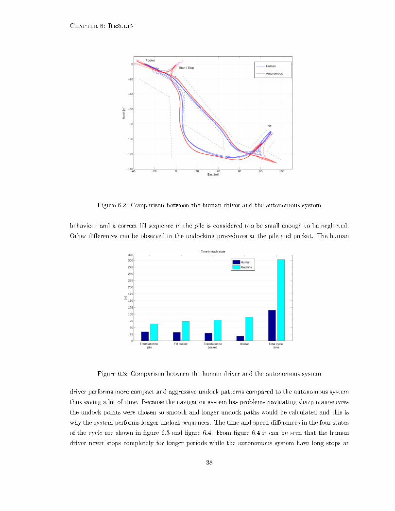
In �gure 6.2 the paths driven by the human and the autonomous system can be seen. At the pile a
problem with the autonomous system can be observed.
A bug in the vision system produced faulty loading points so the machine never �lled the bucket in
the pile, however the bucket �ll sequence were performed in the air. The time di�erence between this
37
Chapter 6: Results
−40 −20 0 20 40 60 80 100−140
−120
−100
−80
−60
−40
−20
0
East [m]
Nor
th [m
]
Start / Stop
Pile
Human
Autonomous
Figure 6.2: Comparison between the human driver and the autonomous system
behaviour and a correct �ll sequence in the pile is considered too be small enough to be neglected.
Other di�erences can be observed in the undocking procedures at the pile and pocket. The human
1 2 3 4 50
25
50
75
100
125
150
175
200
225
250
275
300
320Time in each state
[s]
Human
Machine
Translation to pile
Fill bucket Translation to pocket
Unload Total cycle time
Figure 6.3: Comparison between the human driver and the autonomous system
driver performs more compact and aggressive undock patterns compared to the autonomous system
thus saving a lot of time. Because the navigation system has problems navigating sharp manoeuvres
the undock points were chosen so smooth and longer undock paths would be calculated and this is
why the system performs longer undock sequences. The time and speed di�erences in the four states
of the cycle are shown in �gure 6.3 and �gure 6.4. From �gure 6.4 it can be seen that the human
driver never stops completely for longer periods while the autonomous system have long stops at
38

Chapter 6: Results
0 20 40 60 80 100
−10
0
10
20
30
[s]
[km
/h]
0 50 100 150 200 250 300
−10
0
10
20
30
[s]
[km
/h]
Translation to pile
Translation to pile Bucket fill Translation to pocket Unload
Translation to pocket
Human driver
Autonomous system
Bucket fill Unload
Figure 6.4: Speed comparison between human driver and the autonomous system.
several parts of the cycle. The stops are needed when the machine takes a scan of the environment
and if these could be removed a lot of time could be saved. The human speed is also more smooth
and it almost looks like the whole cycle is done in one sweep compared to the more choppy speed
curve of the autonomous system. The speed both in reverse and forward are faster when the driver
performs the cycle however the speed of the autonomous system are limited so a safe operation is
ensured.
The productivity of the autonomous system were calculated by dividing the mean cycle time for
the human by the mean cycle time of the autonomous system. The calculations showed that the
productivity of the autonomous system were 37.8% compared to a novice driver thus the productivity
goal of 30% for this thesis has been reached.
6.3 Conclusions
When looking at the diagram in �gure 6.3 it can be seen that the states that took the least amount of
time for the human are the states that takes the longest time for the autonomous system. Especially
looking at the unload state it can be seen that the autonomous system uses �ve times more time to
unload the bucket compared to the human. The state contains fast localisation of the pocket and
precision navigation towards it at the same time as a well synchronised movement of the bucket is
performed, for the human novice driver this is not a problem and the unloading can be performed in
a fast and smooth way. The autonomous system solves these problems in a serial way which takes
a lot more time than the parallel processing done by the human. Not much time were put on the
development of the unload sequence so a redesign of the unload sequence can speed up the cycle a
lot. More time could also be saved easily by implementing more aggressive undock patterns both
39

Chapter 6: Results
at the pocket and the pile. In the translation states it can be seen in �gure 6.2 that the human
and autonomous system drives on approximately the same paths so the only way to save time in
these states is to increase the speed. The navigation system has been tested at higher speeds with
promising results but unleashing a 20 ton machine at high speeds with only a human controlled
emergency break can result in dangerous situations. I believe that the productivity of the system
could be increased to 50%-60% with some simple �xes but the real issue that has no simple �x is
the reliability and robustness of the system.
40

Chapter 7
Future work
After working with this system for the last �ve month I still believe that the base structure of the
whole system needs to be reorganised in a more modular and structured system to be able to reach
the robustness and reliability goals for the future. We have proved that the current system is capable
of performing a simple NCC cycle but to reach the speed and reliability needed for continuous work
at a site it is not �t. The state machine designed in this thesis is built upon the old system and
still have the same latency and information throughput problems as the old one. To overcome these
problems the sensor and especially the laser scanner information needs to be processed and fed
through the system in a di�erent way. In this chapter I will present a new system design that I think
will be able to solve the problems of the old system. The system is just a sketch and is inspired by
Stanley's system presented in chapter 3.
7.1 Proposed system
In this section I will explain the structure of the proposed system and it can be seen in �gure 7.1.
The system is built up of the same layers as Stanley's; the sensor layer, the perception layer and the
planning and control layer. All modules run in parallel witch increases the information throughput
and make the system more dynamic than the serial structure of the state machine.
7.1.1 Interprocess communication
One of the �rst changes that should be done is the way the threads are communicating. To min-
imize complexity the system should run the same operating system on all computers so a general
interprocess communication service can exist throughout the whole system. Easy and fast access to
sensor data must be built in to the system in order to get continuous processing of the sensor data.
I believe that the IPC system has a key role so a thorough research of di�erent IPC toolkits should
41

Chapter 7: Future work
Figure 7.1: Schematic overview of the proposed system
be performed. A comparison of di�erent IPC toolkits can be found in [6] and may be used as a start
to �nd a suitable toolkit.
7.1.2 Sensor layer
The sensor layer is responsible for reading sensor data and perform pre�ltering of the data. The
data is then distributed through the system via the IPC service. The reading and pre�ltering will be
performed in the PIP8 computer and then communicated to the PC where it is distributed through
the IPC service. To avoid time skew of the data the data needs to be timestamped with a common
system clock that is synchronized throughout the system. The sensor layer also contains a map of
the site. This map could be a 3D scan of the site done with the laser scanner.
7.1.3 Perception layer
The perception layer consists of �ve modules; the map builder, obstacle detection, object detection,
pose estimation and bucket pose estimation.
Map builder
In the current system the scans are thrown away as soon as the calculations are complete. Due to
the static environment of the site this is a huge waste of information. In this system the map builder
is constantly fed with the scans form the laser. The laser scanner should be pointed about 20 meters
42

Chapter 7: Future work
in front of the machine and use the translation to produce a 3D perception of the environment. It
uses this information and a SLAM algorithm together with the 3D map of the site to produce a
more updated version of the map. The simultaneous localization and mapping(SLAM) algorithm
will also supply the location of the machine in the 3D map and this information is sent to the pose
estimation.
Obstacle detection
Obstacle detection is a very hard problem but as a start this module can be used to detect static
obstacles such as bumps and holes in the ground. During navigation the laser scanner should be
pointed so it scans a line about 20 meters in front of the machine. The height di�erences can then
be used to detect obstacles and non drivable terrain. Information about upcoming obstacles will be
sent to the local path planner.
Pose estimation
The pose estimation is responsible for �nding the machines position and orientation in the coordinate
frame. The current system uses an Extended Kalman �lter(EKF) to fuse the readings from the
di�erent sensors. The �lter is already prepared to use the positions supplied by the SLAM algorithm
and should be su�cient for the future.
Object detection
The object detection is used to �nd objects such as the pocket or a hauler. This function is only
active during a unload sequence and the obstacle detection need to be turned o� while this module
is active. The location of objects is then forwarded to the local path planner.
Bucket pose estimation
This module is responsible for estimating the position of the bucket. Today the bucket position is
represented by the lift angle and the tilt angle. This gives no information about where the bucket tip
is so a conversion from the angles to the actual positions in the Cartesian coordinate frame would
be more intuitive.
7.1.4 Planning and control layer
This layers consists of a planning part and a control part. The planning part has a knowledge about
the site and can plan ahead. The control part then has the low level control of the machine and is
supplied with commands from the planner. The planning part is run on the PC computers while
43

Chapter 7: Future work
the controllers is run on the PIP8 computer. The controllers in the PIP8 only provides a simple
interface where control signals can be streamed down to the regulators.
Pile manager
In the current system the search for a dig point is initiated when the machine has reached the pile
area and a scan is received. This is both a waste of time and information, the job for the pile
manager is to use the 3D scan of the site and prepare a set of suitable dig points in advance. In this
way the pile manager can also control the structure of the pile so the machine does not dig in the
same area every time. The information about the most suitable dig point is then supplied to the
global path planner.
Global path planner
The global path planner uses the 3D map of the site and creates roads between the pockets and
the piles. It has information about the most suitable dig points form the pile manager so it can
create paths straight to the dig point in every pile. A bucket �ll and unload activation point is also
programmed into the path so a state change can occur when they are reached. The roads are then
recalculated every time something changes. The roads are then supplied to the local path planner.
Local path planner
The local path planner is the one that sews all the information together. It uses the road created
by the global path planner as a high level navigation goal but it also uses the information from the
obstacle handler to make small course changes if necessary. The local path planner �nds a drivable
path in the area 20-30 meters in front of the machine and produces steer and velocity commands to
the controllers so the path can be followed. During a unload sequence it receives the location of the
pocket or hauler from the object detector and calculates a path for the bucket which is supplied to
the bucket controller.
Steer controller
The steer controller receives a stream of commands from the local path planner. The controller
regulates the waist angle of the machine and the commands are executed without any concern so
it's up to the local path planner to create feasible commands.
Throttle/Brake controller
To have a good throttle and brake control is important in order to have full control of the machine.
The controller needs to have simultaneous control of both brake and throttle and then use both
44

Chapter 7: Future work
brake and throttle to produce the desired output. The controller has two input control parameters,
the desired velocity and a desired rpm for the engine. The rpm control signal is supplied by the
bucket control system which sometimes need a higher rpm to be able to lift the bucket at the desired
speed. This controller is probably one of the more advanced in this system due to the nonlinear
behaviour of the brake. A good model must be developed and a lot of research is probably needed
to get a working regulator.
Bucket controller
The bucket controller controls the movement of the bucket. Just like the steer controller it has a
stream of control signals that is executed without concern. If the speed of the bucket is too low it will
be regulated by desiring a higher rpm from the throttle and brake controller. To get very accurate
control of the nonlinear hydraulic system a lot of research is needed, however I don't believe that
extremely accurate control of the bucket is necessary to reach the goals. Non of the tasks performed
with the bucket needs very accurate control if enough safety margin is used.
Bucket �ll controller
Some modi�cations should be performed to the bucket �ll controller so it works together with the
rest of the system. The current controller has full control over velocity, rpm, steering and the bucket
which makes it work as a separate part of the system and this makes the design a bit messy. During
a bucket �ll in the new system the local path planner will still be responsible for the movement of
the machine and the bucket �ll controller will only send commands to the bucket controller. In this
way the bucket �ll controller gets a clean interface and works together with the system instead as a
separate system.
7.1.5 Top level control
If the design of the system was done in this way the toplevel control of the system could be simpli�ed
a lot. The statemachine only needs four states in this design and only provides a high level goal to
the system. The statemachine receives a workorder from the site controller containing a pile ID and
a pocket ID. During the translation to pile state it gives the pile ID to the global path planner that
in turn supplies the local path planer with the path to that pile. When the bucket �ll activation
point is reached it will change state to the bucket �ll state. In this state the obstacle avoidance is
ignored and the bucket �ll regulator is activated. When the bucket �ll is complete the translation
to pocket state will supply the global path planner with a pocket ID and a navigation to this point
will start. When the unload activation point is reached the obstacle avoidance is ignored but the
object detection is activated. The local path planner will now calculate a path both for the machine
and for the bucket in order to unload the bucket.
45

Chapter 7: Future work
7.2 Summary
In this chapter I presented a new design that can make the system more �exible and dynamic. To
implement the full design a lot of development and research must be done but if the design is followed
it can be implemented in steps with simpler blocks that can be easily changed when a new module
is developed. If only one part of this system would be implemented I believe that the map builder
and pile manager would have the most positive impact on the current system. The current systems
spends a lot of time just waiting to get the pile examined when this already could have been done
while we were navigating to the pile.
46

Chapter 8
Conclusions and summary
The system performed quite well and the productivity goals were met, however problems with
robustness and reliability can be found in the system. I believe that the productivity of the system
could be increased by simple means to around 50%-60% but to solve the problems with robustness
and reliability I see the need for a redesign where considerations about robustness is taken into
account from the bottom and up. To achieve safe operation and to be able to increase the velocity
during navigation a continuous vision feedback stream is needed so the navigation does not solely
depend on waypoint paths and a correct positioning of the machine.
Modularity and �exibility of the design are also important for the ease of future development. The
developed system in this thesis o�ers some more �exibility but yet again I believe that a redesign is
necessary to get the �exibility wanted for the future.
Even though there are many issues with the system one must keep in mind that the Autonomous
Machine project was never started with the intention to build a commercial system but to show that
it's possible to build autonomous machines with work only done by students. However I believe that
the system could be a lot more organized and structured if documentation were created continuously
and a complete design plan with the di�erent systems were developed from the beginning. We have
proved that it's possible to perform a complete cycle but a lot of work is needed before we see
autonomous wheel loaders on site. Autonomous machines might be the next big revolution in the
construction equipment industry and to fall behind now might leave you there for good therefore I
hope more funding is given to this project so the research can continue.
47

Bibliography
[1] Robin Lilja. Localisation and Navigation of an Autonomous Wheel Loader. Thesis work at
Malardalen University, l 2011.
[2] Rodney A. Brooks. A Robust Layered Control System For A Mobile Robot, March 1986.
[3] Jonathan Connell. A Colony Architecture for an Arti�cial Creature. Massachusetts Institute of
Technology Arti�cial Intelligence Laboratory, l 1989.
[4] Gat Erann. Three-layered architectures. AI-based mobile robots: Case studies of successful robot
systems, pages 195�210, 1998.
[5] S. Thrun, M. Montemerlo, H. Dahlkamp, D. Stavens, A. Aron, J. Diebel, P. Fong, J. Gale,
M. Halpenny, G. Ho�mann, K. Lau, C. Oakley, M. Palatucci, V. Pratt, P. Stang, S. Strohband,
C. Dupont, L.-E. Jendrossek, C. Koelen, C. Markey, C. Rummel, J. van Niekerk, E. Jensen,
P. Alessandrini, G. Bradski, B. Davies, S. Ettinger, A. Kaehler, A. Ne�an, and P. Mahoney.
Stanley: The Robot that Won the DARPA Grand Challenge. Journal of Field Robotics, 23:
661�692, June 2006.
[6] Jay Gowdy. A Qualitative Comparison of Interprocess Communications Toolkits for Robotics,
2000.
[7] Jane Yen Carlo H. Sequin, Kiha Lee. Fair, G2- and C2-continuous circle splines for the interpo-
lation of sparse data points. Computer-Aided Design, 37:201�211, 2005.
[8] http : //en.wikipedia.org/wiki/UML_state_machine.
48

Appendix A
Circle splines
A.1 Circle splines
Circle splines can be used if you have N points and want to calculate a smooth path between these
point. In [7] they present an algorithm for circle splines that uses a trigonometric circle blending
technique. This appendix is a short summary of this article. The concept is shown in �gure A.1. To
Figure A.1: Picture of the PIP8 industrial computer
calculate the path between point p2 and p3 we need the previous and following point. Two circles
are then created, one which intersects points p1, p2 and p3 and one that intersects points p2, p3 and
p4. These circles are then blended with a weighting function that gives higher weight to circle one
close to point p2 and gives a higher weight to circle two closer to point p3. In this way a smooth arc
is created with the tangents in the end points pointing towards points p1 and p4. The algorithm is
described in detail in the next section.
A.1.1 Algorithm
The problem formulation is shown in �gure A.2.
We start by calculating the unit vectors:
49

Appendix A: Circle splines
Figure A.2: Picture of the PIP8 industrial computer
~a =pi − pi−1
|pi − pi−1|~b =
pi+1 − pi|pi+1 − pi|
~c =pi+1 − pi−1
|pi+1 − pi−1|(A.1)
~d =pi+2 − pi+1
|pi+2 − pi+1|
~e =pi+12 − pi|pi+2 − pi|
Next we calculate the tangent angles at pi and pi+1:
τi = arccos (~a • ~c)
τi+1 = arccos (~e • ~d) (A.2)
The blending between the two tangent angles is done with the trigonometric blending function:
τ(u) = τi cos2(uπ/2) + τi+1 sin
2(uπ/2) (A.3)
Where u is a parameter that goes from 0 to 1. A point P (u) on the arc between pi and pi+1 can
now be described as a distance f(u) from point pi and a deviation angle φ(u) form ~b with the
parametrized equations. This can be seen in �gure A.2(b).
f(u) = bsin(uτ(u))
sin(τ(u))(A.4)
φ(u) = (1− u)τ(u) (A.5)
By running this algorithm on all your points and then adding the produced arcs you get a smooth
curve that travels through all points.
50

Appendix B
UML statemachine
B.1 De�nition
A general de�nition of a state machine is: "a state machine is any device that stores the status of
something at a given time and can operate on input to change the status and/or cause an action or
output to take place for any given change". With this de�nition a state machine can be anything
from a light switch to a complete airplane control system. A state machine is said to be built up of
the following elements.
- A set of states
A set of input events
-- A set of output actions
- A function that maps states and input to output actions
- A function that maps states and inputs to states
- A description of the initial state
A state is a unique condition in which the state machine can exist during its life time. For the case
of a light switch the states can be as simple as on and o�. An event is something that happens to
the state machine, it can be the event that someone pushes the button on the light switch. The
function that maps the states and inputs to states is a list of transitions; a transition describes how
the state machine should behave in response to an event based on its current state. For the light
switch di�erent transitions occurs when the button is pressed depending on which state the machine
is currently in, if it is in state on the transition is to state o� and vice versa. The function that
maps states and inputs to output actions is a list of actions that should be performed for a given
state and input, in the light switch case di�erent actions should be performed depending on state
51

Appendix B: UML statemachine
and event. If the switch is in its o� state and a button pressed event is triggered the machine should
transition to the on state and perform a power on action. There are a number of de�ned types of
actions that can be performed:
- Entry action: This action is performed when a state is entered
Exit action: This action is performed when a state is exited
-- Input action: This action is performed depending on present state and input conditions
- Transition action: This action is performed during a transition
B.2 Mealy and Moore
State machines are often divided into two basic models, either a Mealy or a Moore machine. There
is a di�erence between the two but one model can always be converted into the other, the choice
of model will have in�uence on the design but you can't say one is better than the other. In fact
a mix between the two is often used in practice. In the de�nition of a Moore machine there only
exists Entry actions which makes the output only depend on the current state. A Mealy machine
only uses Input actions which makes the output depend on both the state and input. The Moore
machine often needs more states that the Mealy machine.
B.3 UML statemachine
To overcome the main limitations of the traditional state machine UML has introduced an extended
de�nition introducing new concepts such as hierarchically nested states and orthogonal regions.
Below some useful additions are explained.
B.3.1 Extended state machine
In the UML standard an extended state machine is a machine that is supplemented with some
variables and guards. A guard is a simple Boolean evaluation that has to be true or false before a
transition or action is allowed to happen. To give an example of a system where variables and guards
are good to use we can think of a system that counts the number of keystrokes from a keyboard and
after 10000 strokes the system tells the user to take a break. To implement this without variables
we would need over 10000 states, one state for every number of strokes hit so far. This becomes
unpractical very fast but with the use of a guard and variable the system can be implemented as in
Figure B.1:
52

Appendix B: UML statemachine
Figure B.1: Picture of the PIP8 industrial computer
B.3.2 Hierarchically nested states
The biggest addition to the UML state machine compared to the traditional state machine is the
concept of hierarchically nested states. The concept is pretty simple; states can contain states called
substates so a nested structure of states can be created. A state that contains states is called a
composite state. This makes it harder to say which state the machine is in because it can actually
be in several states at the same time, its superstates and substate. A superstate is a state above
the current state in the hierarchy. The nesting provides a great way of sharing behaviour among
several states. An event in a nested state machine is �rst handled by the substate, if the substate
has no description of how to handle the event the event will be sent to its superstate where it might
be handled. An event can be sent all the way to the top of the hierarchy but the handling always
starts in the current state and gets sent up the tree. A calculator example is explained below??.
If we were to design the calculator using a traditional state machine we would get a design as in
Figure B.2: As we can see a lot of transitions are the same no matter which state you are currently
Figure B.2: Implementation of calculator using traditional state machine design.
in. In this case you have to specify the transitions in every states transition table. The C and OFF
events are certainly states that are shared between all the states, this is a typical situation where
the advantages of a nested structure is shown. In �gure B.3 a nested design of the same calculator
are shown. In this design we see that there is one super state, ON and its di�erent substates that
handles the actual calculator. Here the only state that needs to handle the C and OFF state is
the superstate ON. If a C or OFF event occurs the current substate have no speci�cation of how
53

Appendix B: UML statemachine
Figure B.3: Implementation of calculator using nested state machine design.
to handle that event and therefore the event is sent to its super state, ON, where it is handled in
the correct manner. This structure gives the opportunity to program the state machine with the
concept of programming by di�erence. Instead of creating a new state every time, you only de�ne
the di�erences from its super state. This type of inheritance is called behavioural inheritance.
B.3.3 Entry and Exit actions
Every state in the UML standard can have an entry action which is executed on entrance to the
state and an exit action which is executed when exiting the state. Regardless of how the state is
entered or exited the actions will always execute. This provides a great way of dealing with the
initialization and cleanup in every state. When programming a UML state machine the allocation
and deallocation of memory would be a great examples of how to use these actions.
B.3.4 Orthogonal regions
An orthogonal region gives a composite state the ability to be in two independent states at the same
time. This is used when you have behaviour that is completely independent from each other in the
same super state. An example of this could be a keyboard, it has two independent regions. One
region for the numerical keypad which can be both in arrow or numerical mode and one region for
the main keyboard which can be in the modes caps locked or default mode. In �gure 6 this system
is shown. Here the states in the orthogonal regions can change independent of each other. This is
Figure B.4: Example of orthogonal states.
often implemented in software using a threaded design.
54

Appendix C
.NET State Machine Toolkit
The toolkit has no fancy name but it implements most of the functions described in the UML-
statemachine and it is easy to use. The toolkit was developed by Leslie Sanford and released under
the CPOL licence which allows use of the code in commercial projects. To get a taste of how
the toolkit works I will explain it through a small example. We will look at a automatic door
statemachine. The door can either be in state opened or closed and the door can be opened if's in
the closed state or closed if it's in the opened state.
First we de�ne the base of the statemachine. To start with we de�ne the identi�cation number foreach state and for each event by de�ning two enumerations, StateID and EventID. We then de�nethe AutomaticDoor class which inherits the behaviour from the ActiveStateMachine that is de�nedin the toolkit. When this is done we de�ne a constructor, the states and �nally the entry and exitmethods for each state. The code can be found below.
enum class StateID{Open , Closed } ;
enum class EventID{Close , Open} ;
public r e f class AutomaticDoor : ActiveStateMachine
{
public :
AutomaticDoor ( ) ;
private :
State ^Open , ^Closed ;
void EntryOpen (void ) ;
void EntryClosed (void ) ;
void ExitOpen (void ) ;
void ExitClosed (void ) ;
}
The next stage is to implement what we de�ned before. In the constructor the behaviour of the
55

Appendix C: .NET State Machine Toolkit
statemachine is de�ned. To start with we instantiate the states and give them a handle to a entryand a exit method that will be called when the state is entered and exited. The transitions betweenstates is then easily de�ned by binding a transition to a event in each state. The structure of thestate machine is now complete.
AutomaticDoor ( ){
Open = gcnew State ( ( int ) StateID : : Open , gcnew EntryHandler ( this ,&EntryOpen ) ,
gcnew ExitHandler ( this ,&ExitOpen ) ) ;
Closed = gcnew State ( ( int ) StateID : : Closed , gcnew EntryHandler ( this ,&EntryClos
ed ) , gcnew ExitHandler ( this ,&ExitClosed ) ) ;
Trans i t i on t rans ;
t rans = new Trans i t i on ( Closed ) ;
Open . Trans i t i on s .Add( ( int ) EventID . Close , t rans ) ;
t rans = new Trans i t i on (Open ) ;
Closed . Trans i t i on s .Add( ( int ) EventID .Open , t rans ) ;
I n i t i a l i z e ( Closed ) ;
}
void EntryOpen (void ){
Console : : WriteLine ( "Enter ing Open" ) ;
}
void EntryClosed (void ){
Console : : WriteLine ( "Enter ing Closed " ) ;
}
void ExitOpened (void ){
Console : : WriteLine ( " Exi t ing Opened" ) ;
}
void ExitClosed (void ){
Console : : WriteLine ( " Exi t ing Closed " ) ;
}
}
The state machine can now be used by creating a instance of the automatic door and sending eventsto it.
void Main( s t r i n g [ ] a rgs )
{
AutomaticDoor ad = new AutomaticDoor ( ) ;
l s . Send ( ( int ) AutomaticDoor . EventID .Open ) ;
l s . Send ( ( int ) AutomaticDoor . EventID . Close ) ;
l s . Send ( ( int ) AutomaticDoor . EventID .Open ) ;
56

Appendix C: .NET State Machine Toolkit
l s . Send ( ( int ) AutomaticDoor . EventID . Close ) ;
}
The output from the code above is shown here.
Enter ing Closed
Exi t ing Closed
Enter ing Open
Exi t ing Opened
Enter ing Closed
Exi t ing Closed
Enter ing Open
Exi t ing Opened
Enter ing Closed
57


