A STATISTICAL APPROACH TO VIEW SYNTHESIS

by

PHILLIP ELLIOTT BERKOWITZ B.S. University of Central Florida, 2005

A thesis submitted in partial fulfillment of the requirements for the degree of Master of Science

in the Department of Electrical and Computer Engineering in the School of Electrical Engineering and Computer Science

at the University of Central Florida Orlando, Florida

Summer Term 2009

Major Professor: Mubarak Shah

© 2009 Phillip Berkowitz

ii

ABSTRACT

View Synthesis is the challenging problem of predicting a new view or pose of an

object given an exemplar view or set of views. This thesis presents a novel approach for

the problem of view synthesis. The proposed method uses global features rather than

local geometry to achieve an effect similar to that of the well known view morphing

method [1].

While previous approaches to the view synthesis problem have shown impressive

results, they are highly dependent on being able to solve for epipolar geometry and

therefore have a very precise correspondence between reference images. In cases where

this is not possible such as noisy data, low contrast data, or long wave infrared data an

alternative approach is desirable.

Here two problems will be considered. The proposed view synthesis method will

be used to synthesis new views given a set of reference views. Additionally the

algorithm will be extended to synthesis new lighting conditions and thermal signatures.

Finally the algorithm will be applied toward enhancing the ATR problem by creating

additional training data to increase the likelihood of detection and classification.

iii

I dedicate this work to all of my family and friends that continued to support

me throughout the last two years even though I was largely unavailable in many ways while working on my graduate degree.

iv

ACKNOWLEDGMENTS

I would like to thank my advisor Dr. Mubarak Shah for allowing me to be part of

his research group without any experience in his area of research and being patient with

me during my development, and not giving up on me after all of this time. I would also

like to acknowledge Dr. Abhijit Mahalanobis for taking so much time out of his schedule

to guide me with my thesis research. Additionally I would like to thank my committee

Dr. Sam Richie and Dr. Marshall Tappen not only for attending my committee but for

being a big part of my educational development throughout my coursework.

v

TABLE OF CONTENTS

LIST OF FIGURES ....................................................................................................... VIII

LIST OF TABLES............................................................................................................. X

LIST OF ACRONYMS .................................................................................................... XI

CHAPTER ONE: INTRODUCTION................................................................................. 1

Previous Work ................................................................................................................ 1

Problem Statement .......................................................................................................... 1

Overview......................................................................................................................... 3

Organization of the Thesis.............................................................................................. 5

CHAPTER TWO: RELATED WORK............................................................................... 7

View Morphing............................................................................................................... 7

Pre-warping................................................................................................................. 8

Correspondence....................................................................................................... 8

Epipolar Geometry.................................................................................................. 9

Rectification.......................................................................................................... 10

Morphing................................................................................................................... 11

Post-warping ............................................................................................................. 12

Limitations of View Morphing ..................................................................................... 13

Detection and Classification ......................................................................................... 16

Correlation using MACH.......................................................................................... 16

Support Vector Machines ......................................................................................... 20

CHAPTER THREE: PROSPOSED VIEW SYNTHESIS METHOD.............................. 26

vi

Mathematical Formulation............................................................................................ 26

Creating a Predictor ...................................................................................................... 29

Novel Views Prediction ................................................................................................ 32

Novel Signature Prediction........................................................................................... 35

Sources of Data Degradation ........................................................................................ 38

Sensor Type .............................................................................................................. 39

SNR: Its Affect on Synthesis .................................................................................... 40

Noisy Data ............................................................................................................ 40

Low Contrast or Blurred Data............................................................................... 42

CHAPTER FOUR: EXPERIMENTS & RESULTS......................................................... 43

Datasets......................................................................................................................... 43

Experiments .................................................................................................................. 45

Varying the Number of Basis Vectors Used to Create the Predictor........................ 45

Prediction Quality as a Function of Added Noise and Blur...................................... 47

Predicting Views from a New Signature Type ......................................................... 48

CHAPTER FIVE: CONCLUSION................................................................................... 50

Summary....................................................................................................................... 50

Future Work.................................................................................................................. 51

LIST OF REFERENCES.................................................................................................. 53

vii

LIST OF FIGURES

Figure 2-1: A Point in 3d space as seen from epipolar geometry...................................... 9

Figure 2-2: Using the Fundamental Matrix to map a point to a line................................. 11

Figure 2-3: The non-rectified image interpolation problem.. ........................................... 12

Figure 2-4: A view rectification example with no deformities......................................... 13

Figure 2-5: A view rectification example with blur and noise added............................... 14

Figure 2-6: Training and testing data for MACH experiments......................................... 18

Figure 2-7: Resultant MACH filter................................................................................... 18

Figure 2-8: Results for first experiment using MACH filter. ........................................... 19

Figure 2-9: Results for second experiment using a single ‘X’.......................................... 20

Figure 2-10: Linearly separable two class classification problem.................................... 21

Figure 2-11: Non-linearly separable two class classification problem............................. 22

Figure 2-12: A sample of the characters from the NIST handwriting database [30]........ 24

Figure 2-13: Histogram of characters from training and testing dataset .......................... 24

Figure 3-1: Virtual cameras representing multiple views of an object. ............................ 30

Figure 3-2: Estimating a view from an arbitrary image.................................................... 33

Figure 3-3: Block diagram of linear prediction with feedback......................................... 35

Figure 3-4: Comparison of thermal signatures.. ............................................................... 37

Figure 3-5: Problem images for automatically finding and refining correspondences..... 39

Figure 3-6: Effects of noise and blur on feature point correspondence............................ 41

Figure 4-1: This figure shows subsets of the major datasets used in this paper ............... 44

Figure 4-2: Results from experiment 1. ............................................................................ 46

viii

Figure 4-3: Results from experiment 2. ............................................................................ 47

Figure 4-4: Results from experiment 3. ............................................................................ 49

ix

LIST OF TABLES

Table 2-1: Affect of image deformity on accuracy of epipolar geometry ........................ 15

Table 2-2: Types of kernels used in SVM ........................................................................ 23

Table 2-3: Results for SVM character classification ........................................................ 25

Table 3-1: Comparison of model with principle component reduction vs. no reduction . 34

x

LIST OF ACRONYMS

ATR

CAD

EO

IBR

IR

KL

LLS

MACH

MMSE

PCA

PSR

RANSAC

SIFT

SNR

SVM

Automatic Target Recognition

Computer Aided Design

Electro-Optic

Image Based Rendering

Infrared

Karhunen Loeve

Linear Least Squares

Maximum Average Correlation Height

Minimum Mean Squared Error

Principle Component Analysis

Peak to Side Lobe Ration

Random Sample Consensus

Scale Invariant Feature Transform

Signal to Noise Ratio

Support Vector Machine

xi

CHAPTER ONE: INTRODUCTION

Previous Work In many pattern recognition applications, it becomes necessary to predict the

shape or appearance of an object from several views. It is imperative to estimate new

views of an object under varying imaging conditions, such as when there are changes in

lighting and thermal levels, or when the viewing geometry has shifted. Specifically, the

goal is to estimate a singular view of the object consistent with any imaging conditions

present in the reference view. For example, an object that has already been examined for

training data in several ways could potentially yield new data in subsequent observations.

In IR, the thermal condition of the new exemplar of an existing object could be

drastically different from the training data, requiring views from the new condition to be

estimated. Similarly in visible images, conditions in illumination could alter the

appearance of the object to such a degree that standard classification algorithms would

have difficulty recognizing it. In this case, the new illumination condition would also

need to be estimated.

Problem Statement

Of course many methods have been proposed in attempts to address these types of

challenging problems before. In the most general case where prior information about the

object is unavailable, conventional approaches may extract edges and employ wire frame

1

models. These tactics geometrically manipulate the data in a 3D sense. Alternately

epipolar geometry could be solved for by first solving precise correspondence between

reference images. Once the geometry is known, pre- and post-warping could be used to

interpolate synthetic images of a view between the reference views. This is known as

view-morphing [1] and will be further discussed in CHAPTER TWO. This thesis deals

with a more bounded problem where is it assumed that the prior knowledge about the

object (such as representative views) is available.

We are concerned with estimating or predicting new views of the same object.

This concept is known in general as View Synthesis although specific implementations

may take on other names. Previously established methods can work well in many

situations. View-morphing for example can create very realistic synthesized views based

off of reference images.

In order to use the traditional approaches, regardless of which implementation is

chose, they all seem to require establishing precise correspondence between reference

images an initial step. At the time of this thesis the state of the art method of finding this

type of accurate correspondence without human interaction was to first use feature point

correspondence such as SIFT [11] followed by a refinement step to remove outlier

matches keeping only the most likely correspondences using a method like RANSAC

[13].

While this type of technique might be convenient in many types of images, there

are several applications where this technique will fail. Such applications would include

applications with various amounts of noise present in the data, motion blur present in the

2

data, low contrast data, and most long wave infrared data. Although manual

correspondence could be used to get around this problem, it is not only tedious but in

many cases unreliable due to the lack of precision accompanied by manual selection.

CHAPTER THREE will examine data types in much detail and show how the ability to

accurately discover correspondence in pairs of reference images deteriorates with

different types of data.

Overview

In this thesis we describe a novel approach to the view synthesis problem, one

that does not depend at all on image correspondence or epipolar geometry. The approach

was motivated by two major considerations. The first consideration is the need for multi-

view-morphing similar in concept to [18] for boosting a learning algorithm with the

ability to generate high-quality synthesized views which are not stored in the training set.

This concept was accomplished using a modified view-morphing technique known as tri-

view-morphing [7], however as mentioned prior, it depends on precise correspondence.

The IR and noisy data are what is motivating a new approach to that problem. The

second consideration is the case where we have images spanning the set of needed views

already in the training database. The goal here is to predict views of that object from new

thermal or illumination conditions. Therefore looking at the two major considerations for

the proposed view-synthesis method, it becomes clear that it would be better suited and

more appropriate to restrict the use of this algorithm to applications that are limited by

low contrast or damaged data.

3

More specifically our approach is able to solve the problem without

correspondence and epipolar geometry by treating the problem as a 2-D linear prediction

process. As previously mentioned, it is assumed that the representative training views of

the desired object are available. The first step is obtaining a basis set representing the

training data, which is accomplished in this thesis by computing the Karhunen Loeve

(KL) expansion of the data. The training images are represented in terms of their

principle components (although other basis representations could be used). Purportedly,

using the principle components will constitute a reasonable basis for the unknown views.

This assumption implies that there is a certain amount of similarity between the predicted

view and the training data. The projections of the training images onto the basis set are

treated as features that will be used for estimating the linear predictor. It is well known

that the number of principle components may be reduced while still well representing the

data. Using fewer principle components allows a predictor to be estimated with less

training data. Then given an arbitrary image of the object, its features can be the input

for the linear predictor which will estimate the output features of the desired synthesized

view. The features can either be reconstructed into an image of this view, or left in

feature-space to be classified if the actual image is not required. In addition to creating

and using a linear predictor to estimate the appearance of the object from new views, this

approach can also effectively estimate new signatures. These signatures can be

illuminations or lighting conditions in visible data or could be thermal states in IR data.

This effort may be accomplished simply by adding data from multiple signature types

and using the new training data to create the basis set and estimate the predictor.

4

While the main problem to be solved by this thesis is to synthesize new views and

signature types, it is not the only focus. Other literature such as Xiao et al [18] have used

synthesized or morphed views to enhance the performance of Automatic Target

Recognition. Since one of the motivations of this thesis was to focus on data that is noisy

or low contrast, it seemed natural to try to apply this to the ATR problem; a problem

which commonly has IR data or long range-data with noise present. This thesis will use

the proposed method of synthesis to enhance completely independent approaches to the

ATR problem and show promise.

Organization of the Thesis

The remainder of the thesis is organized as follows. CHAPTER TWO: will

review previous approaches to view synthesis problem along with some intermediate

results showing when it can be successfully used as well as when it will not be effective.

This will demonstrate the motivation for the proposed method. In addition to reviewing

other approaches, it is necessary to review some prerequisite related works that were

needed to develop the proposed solution and to run all subsequent experiments.

CHAPTER THREE will develop the view-synthesis problem as a prediction process in

terms of predicting the principle component-based features. This effect will be evident

when a system of linear equations is established by relating the principle component

features of different views. A minimum mean square error (MMSE) model can be solved

for using well-known regression techniques. This portion will conclude with a

demonstration of this model to estimating new views and new signature types.

5

CHAPTER FOUR contains all of the experiments performed in this thesis. It will show

examples of the proposed view-synthesis approach used on data to predict views as well

as predict new signature conditions. Additionally there will be an example using the

predicted views in an ATR application. Finally CHAPTER FIVE will summarize the

thesis making conclusions that compare these experiments performed to other

approaches. This section will also discuss future directions and applications for our

findings.

6

CHAPTER TWO: RELATED WORK

Several disciplines have approaches to solving the Image Based Rendering

problem. The two predominant ones are computer graphics and computer science. Each

of them has their own associated advantages and disadvantages. It is important to

understand the state-of-the-art approaches at some level to better appreciate the work and

contribution in this thesis. This chapter will begin by reviewing one of the more popular

approaches to View Synthesis, showing some results, and demonstrating the motivation

for an alternate solution such as the one proposed. This will be followed by a review of

ATR techniques that will be used in later chapters.

View Morphing

View Morphing [1], [20], [1] as described by Seitz, is the problem of synthesizing

realistic images of a real scene from new virtual camera view points by warping a pair of

basis images. The algorithm should be able to produce convincing novel views as long as

the constraints are satisfied while being versatile enough to handle change in lighting and

non-static scenes. The main constraints being that a reasonable correspondence can be

solved for or manually provided such that the epipolar geometry can be recovered.

Additionally, only a minimal amount of occlusion may be present or artifacts will be

introduced making the synthesized results not very convincing. Finally the object of

interest should be rigid between each of the basis images.

7

The main issues resolved by this method, described in [21], are uniqueness, correctness,

registration, uncalibrated cameras, and synthesis. Uniqueness implies that the each novel

viewpoint must be uniquely determined from the basis images. Correctness is used to

state that the resultant image should be reasonable and convincing as if a real, not virtual

camera had seen the object from the new viewpoint. Registration of the basis images

should be possible as mentioned in the above constraint description. This should be

possible without prior knowledge of camera parameters such as position and focal length

making them Uncalibrated Cameras. Synthesis of images should not only be correct by

the above definition of correctness, they should be general enough to work with any

object satisfying the aforementioned constraints. Seitz and Dyer describe a generalized 3

step algorithm for solving these issues in [20]. Below, each of the steps will be described

with some intermediate results shown.

Pre-warping

Pre-warping is a term used by Seitz and Dyer to describe the process of finding

correspondence between the two basis images, using the correspondence to recover the

epipolar geometry, and finally using the epipolar geometry to rectify the images into

parallel images with aligned scan lines.

Correspondence

It is important to be able to establish correspondence between the two basis

images. Correspondence may either be user provided or automatically recovered. It is

8

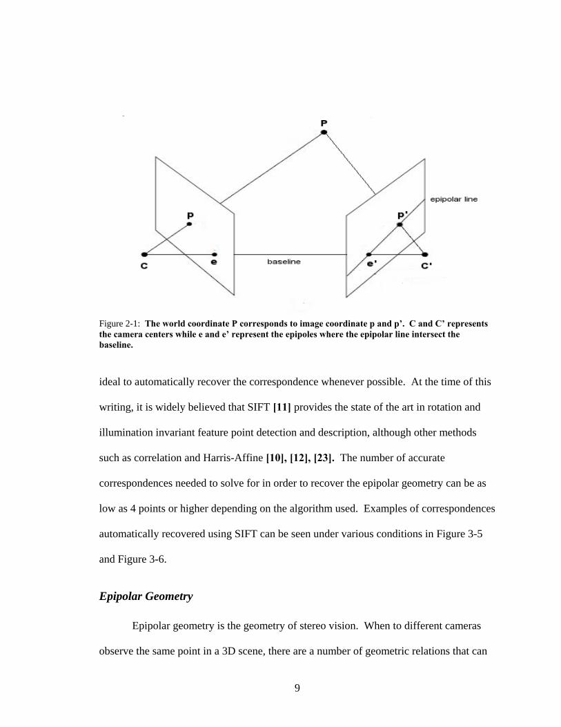
Figure 2-1: The world coordinate P corresponds to image coordinate p and p’. C and C’ represents the camera centers while e and e’ represent the epipoles where the epipolar line intersect the baseline.

ideal to automatically recover the correspondence whenever possible. At the time of this

writing, it is widely believed that SIFT [11] provides the state of the art in rotation and

illumination invariant feature point detection and description, although other methods

such as correlation and Harris-Affine [10], [12], [23]. The number of accurate

correspondences needed to solve for in order to recover the epipolar geometry can be as

low as 4 points or higher depending on the algorithm used. Examples of correspondences

automatically recovered using SIFT can be seen under various conditions in Figure 3-5

and Figure 3-6.

Epipolar Geometry

Epipolar geometry is the geometry of stereo vision. When to different cameras

observe the same point in a 3D scene, there are a number of geometric relations that can

9

be made between the 3D point and its projections onto the 2D images. This can be

observed in Figure 2-1. Corresponding points in the two images can be related by (2-1)

where and ' are corresponding points in the basis images, is the fundamental

matrix

p p F

[24] which can be computed by several algorithms such as Hartley’s 8 point

algorithm [14]. The Fundamental matrix is a 3x3 matrix which represents intrinsic

parameters as well as relative translation and rotation. Using the Fundamental matrix,

Seitz and Dyer can modify these two basis images such that they become parallel views

meaning that their horizontal scan lines are aligned, this process is called rectification.

0'=FppT (2-1)

Rectification

Observing Figure 2-3 (a) you can see that middle image is not a realistic view

between the outer reference images. This incorrect trajectory exists because when

linearly interpolating between two points, interpolation takes place along the most direct

10

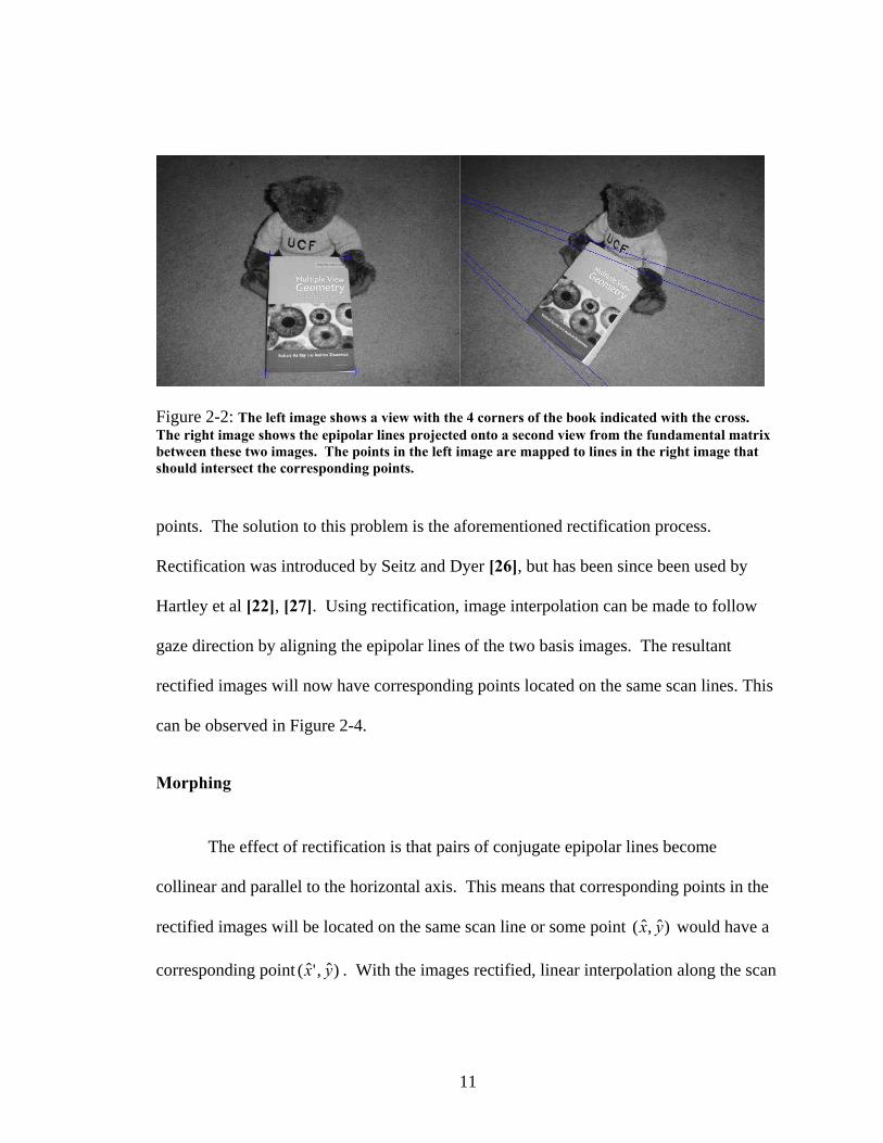
Figure 2-2: The left image shows a view with the 4 corners of the book indicated with the cross. The right image shows the epipolar lines projected onto a second view from the fundamental matrix between these two images. The points in the left image are mapped to lines in the right image that should intersect the corresponding points.

points. The solution to this problem is the aforementioned rectification process.

Rectification was introduced by Seitz and Dyer [26], but has been since been used by

Hartley et al [22], [27]. Using rectification, image interpolation can be made to follow

gaze direction by aligning the epipolar lines of the two basis images. The resultant

rectified images will now have corresponding points located on the same scan lines. This

can be observed in Figure 2-4.

Morphing

The effect of rectification is that pairs of conjugate epipolar lines become

collinear and parallel to the horizontal axis. This means that corresponding points in the

rectified images will be located on the same scan line or some point would have a

corresponding point . With the images rectified, linear interpolation along the scan

)ˆ,ˆ( yx

)ˆ,'ˆ( yx

11

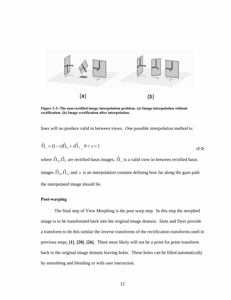
Figure 2-3: The non-rectified image interpolation problem. (a) Image interpolation without rectification. (b) Image rectification after interpolation.

lines will no produce valid in between views. One possible interpolation method is:

10ˆˆ)1(ˆ Π+Π−=Π sss , 10 << s (2-2)

where are rectified basis images, is a valid view in between rectified basis

images , and is an interpolation constant defining how far along the gaze path

the interpolated image should lie.

10ˆ,ˆ ΠΠ sΠ̂

10ˆ,ˆ ΠΠ s

Post-warping

The final step of View Morphing is the post warp step. In this step the morphed

image is to be transformed back into the original image domain. Sietz and Dyer provide

a transform to do this similar the inverse transforms of the rectification transforms used in

previous steps, [1], [20], [26]. There most likely will not be a point for point transform

back to the original image domain leaving holes. These holes can be filled automatically

by smoothing and blending or with user interaction.

12

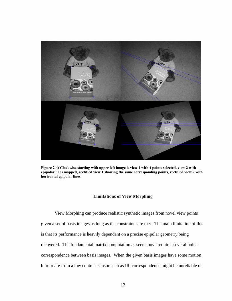
Figure 2-4: Clockwise starting with upper left image is view 1 with 4 points selected, view 2 with epipolar lines mapped, rectified view 1 showing the same corresponding points, rectified view 2 with horizontal epipolar lines.

Limitations of View Morphing

View Morphing can produce realistic synthetic images from novel view points

given a set of basis images as long as the constraints are met. The main limitation of this

is that its performance is heavily dependant on a precise epipolar geometry being

recovered. The fundamental matrix computation as seen above requires several point

correspondence between basis images. When the given basis images have some motion

blur or are from a low contrast sensor such as IR, correspondence might be unreliable or

13

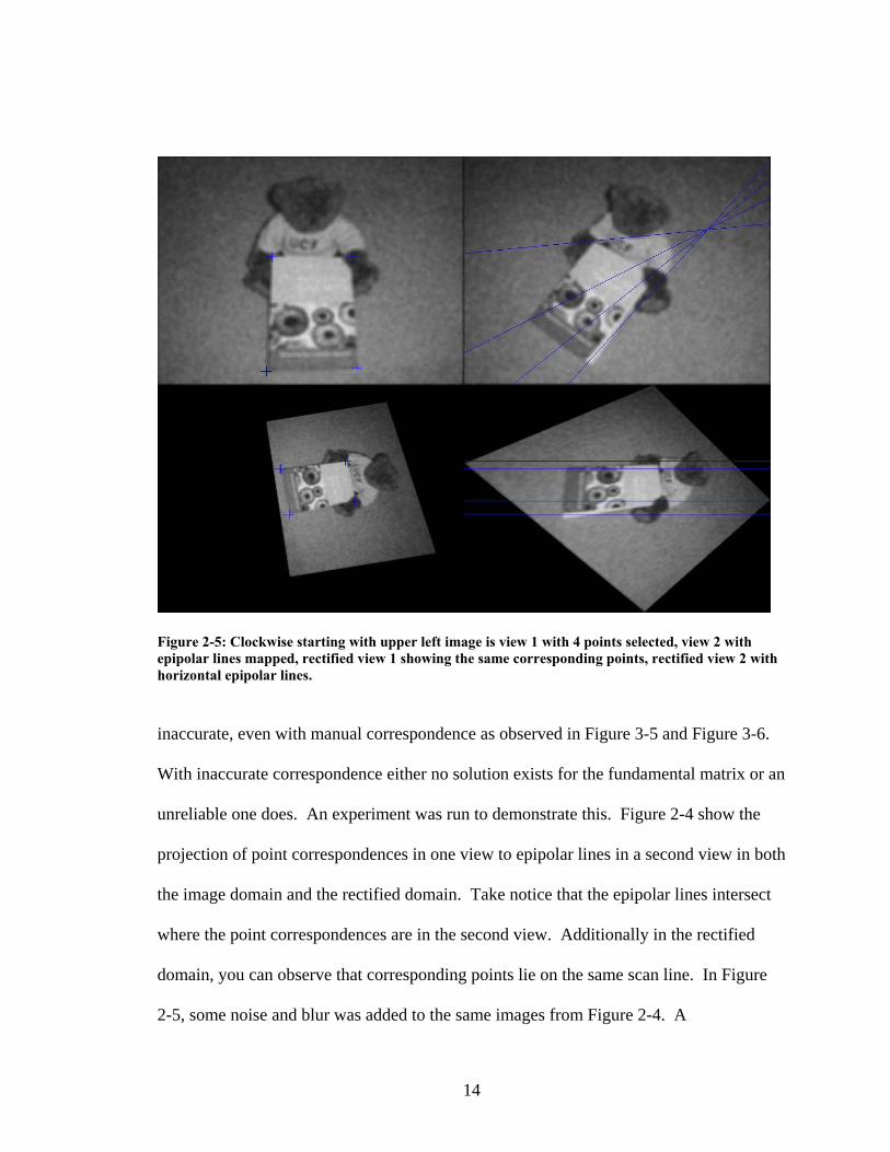
Figure 2-5: Clockwise starting with upper left image is view 1 with 4 points selected, view 2 with epipolar lines mapped, rectified view 1 showing the same corresponding points, rectified view 2 with horizontal epipolar lines.

inaccurate, even with manual correspondence as observed in Figure 3-5 and Figure 3-6.

With inaccurate correspondence either no solution exists for the fundamental matrix or an

unreliable one does. An experiment was run to demonstrate this. Figure 2-4 show the

projection of point correspondences in one view to epipolar lines in a second view in both

the image domain and the rectified domain. Take notice that the epipolar lines intersect

where the point correspondences are in the second view. Additionally in the rectified

domain, you can observe that corresponding points lie on the same scan line. In Figure

2-5, some noise and blur was added to the same images from Figure 2-4. A

14

correspondence procedure was used iteratively with SIFT with RANSAC [13] to ensure

only inlier correspondences were used to solve for the Fundamental matrix. It can be

observed that the epipolar lines do not intersect all of the points they were mapped from,

and in the rectified domain, not all of the corresponding points occur on the same scan

line. This will lead to an incorrect morph since morphing takes place along the scan line

in the rectified domain. Due to the impact of blur and noise on the epipolar geometry it

should be apparent that an alternate method of creating new views that does not depend

on geometry for this type of data. Below Table 2-1 shows the impact of deformities on

the accuracy of the fundamental matrix. The Samson distance is used to measure

accuracy as Gaussian noise and blur are introduced.

Table 2-1: Affect of image deformity on accuracy of epipolar geometry

Deformity Sampson Distance

None 0.2735194725

5x5 Gaussian Blur 0.4055758822

10x10 Gaussian Blur 0.6384753291

15x15 Gaussian Blur 2.0534070628

.025 Variance Noise 0.5182768764

.050 Variance Noise 0.8883337633

.075 Variance Noise 1.1168403824

5x5 Blur + .025 Noise 1.2433494125

5x5 Blur + .050 Noise 7.2159075410

5x5 Blur + .075 Noise 10.1189762729

15

Detection and Classification

While the main focus of this thesis is the proposed View Synthesis algorithm, it is

a hope that using this algorithm to create novel observations of an object will improve

results from well known ATR frameworks. Two such frameworks were chosen, MACH

correlation filters [8] and Support Vector Machines [28]. These frameworks will be

reviewed and demonstrated below.

Correlation using MACH

The correlation based approach requires no image segmentation as compared to a

machine learning classifier due to the fact that it compares the entire image to a template

or filter. In general correlation based approached can suffer from the filter deviating even

slightly from the target. The maximum average correlation height (MACH) filter used by

Mahalanobis et al [8] is a good choice because it can incorporate a set of images into the

filter to allow more variance while maintaining high and sharp peaks. This will give the

MACH filter some view and illumination invariance in correlation assuming the right set

of images was used in the creation of the filter.

Given a set of training images, the MACH filter is given by:

mCSh 1)( −+= (2-3)

16

where represents the average training image, represents the spectral variance of the

data, and C is the power spectrum of the background. Performance for the MACH filter

is measured in terms of peak to side lobe ratio (PSR) which is defined by:

m S

σμ−

=pPSR

(2-4)

where represents the maximum value returned from cross correlation between the filter

and the test image, and

p

μ and σ represent the mean and standard deviation of the cross

correlation respectively. One of the appealing characteristics of the MACH filter was

that accounting for some variation between the filter and the test image, cross correlation

should still return high sharp peaks. That being the case it is expected that the PSR

should be high when an image has qualities similar to the filter and should be low

otherwise.

To demonstrate this, we present an experiment where we will use correlation to

detect and classify an alphanumeric character. We will run the experiment twice, once

with one exemplar character as the correlation template and a second time using many

characters to train a MACH filter. Finally we will compare the resulting correlation maps

as well as detection based on the PSR threshold. Figure 2-1 shows the input for the

experiment. Both experiments will share the left image as a test image to try to find all

instances of the character ‘X”. In the first experiment we will use all of the ‘X’s on the

right side to generate a MACH filter, while in the second we will use the single ‘X” at the

bottom for standard template based correlation.

17

Figure 2-6: The left side shows a test image. The right hand side is the set of characters to train a MACH filter. The single character will be used for standard template based correlation. To create the MACH filter the first step was to interpolate all training images to the same

size. After that we simply apply the equation seen in (2-4). This gives us the MACH

filter represented by Figure 2-7. Once we have this filter we can simply use

Figure 2-7: Resultant MACH filter

18

Figure 2-8: Results for first experiment using MACH filter. The Right shows the correlation map, while the left thresholds PSR to show detection results.

normalized cross correlation as in equation (2-5), where I is the test image and is the h

∑ −−− yx hI

hyxhIyxIn ,

)),()(),((1

1σσ

(2-5)

MACH filter. Figure 2-8 shows the resulting correlation map on the right. Using

equation (2-4) on the correlation map we can computer the PSR for every pixel in the

correlation map and use this value to threshold detections. The left side shows the

detections after applying a threshold. All ‘X’s were detected. The darker red bounding

boxes means that the MACH filter had adjacent pixels with a PSR higher then the

threshold. The second part of this experiment was to repeat the process using normalized

cross correlation using a single ‘X’ as the template and compare results. The results for

this can be seen in Figure 2-9. As expected the filter response was dull compared to the

19

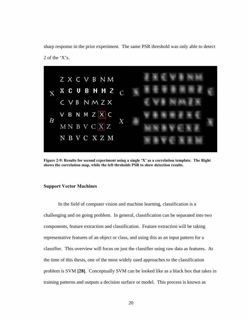
sharp response in the prior experiment. The same PSR threshold was only able to detect

2 of the ‘X’s.

Figure 2-9: Results for second experiment using a single ‘X’ as a correlation template. The Right shows the correlation map, while the left thrsholds PSR to show detection results.

Support Vector Machines

In the field of computer vision and machine learning, classification is a

challenging and on going problem. In general, classification can be separated into two

components, feature extraction and classification. Feature extraction will be taking

representative features of an object or class, and using this as an input pattern for a

classifier. This overview will focus on just the classifier using raw data as features. At

the time of this thesis, one of the most widely used approaches to the classification

problem is SVM [28]. Conceptually SVM can be looked like as a black box that takes in

training patterns and outputs a decision surface or model. This process is known as

20

training. Following training unknown patterns can be presented and compared to this

model and assigned a class and confidence based of how it compared to the model. This

process is known as testing or classifying.

Theoretically, inside of the black box, SVM is hyperplane classifier which will try

to learn a hyperplane that can best separate the input patterns. In the most general case,

consider a two class problem that is linearly separable such as in Figure 2-10. In this case

an optimal linear boundary can be solved using, for example, the perceptron learning

algorithm [31].

0 2 4 6 8 100

5

10

15

20

25

30

35Two Class Classification Problem

wTx+b < 0

wTx+

b >

0

class 1class 2

wTx+b = 0

Figure 2-10: Linearly separable two class classification problem.

21

−4 −3 −2 −1 0 1 2 3 4 5 6−10

−5

0

5

10

15Input Space

−3 −2 −1 0 1 2 3 4 5−10

−5

0

5

10Feature Space

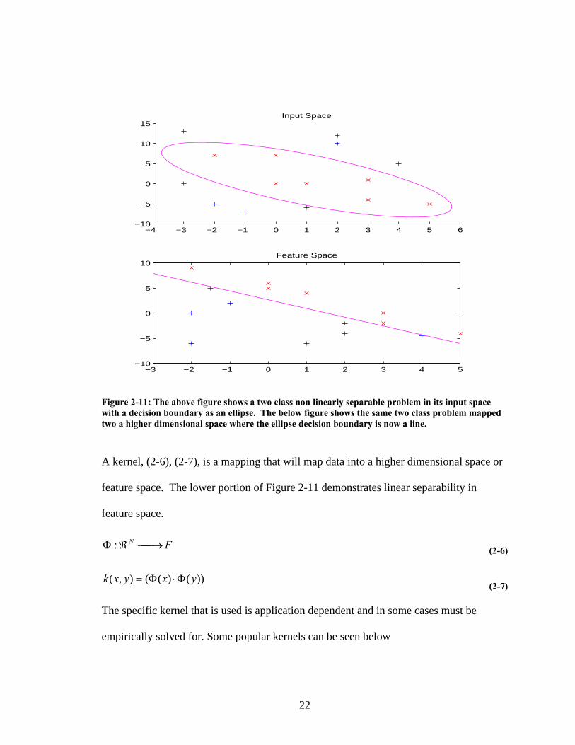
Figure 2-11: The above figure shows a two class non linearly separable problem in its input space with a decision boundary as an ellipse. The below figure shows the same two class problem mapped two a higher dimensional space where the ellipse decision boundary is now a line.

A kernel, (2-6), (2-7), is a mapping that will map data into a higher dimensional space or

feature space. The lower portion of Figure 2-11 demonstrates linear separability in

feature space.

FN ⎯→⎯ℜΦ : (2-6)

))()((),( yxyxk Φ⋅Φ= (2-7)

The specific kernel that is used is application dependent and in some cases must be

empirically solved for. Some popular kernels can be seen below

22

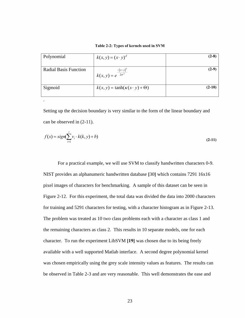
Table 2-2: Types of kernels used in SVM Polynomial dyxyxk )(),( ⋅= (2-8)

Radial Basis Function 2

2

2),( σ

yx

eyxk−−

= (2-9)

Sigmoid ))(tanh(),( Θ+⋅= yxyxk κ (2-10)

.

Setting up the decision boundary is very similar to the form of the linear boundary and

can be observed in (2-11).

∑=

+⋅=l

1)),(()(

ii bykkvsignxf

(2-11)

For a practical example, we will use SVM to classify handwritten characters 0-9.

NIST provides an alphanumeric handwritten database [30] which contains 7291 16x16

pixel images of characters for benchmarking. A sample of this dataset can be seen in

Figure 2-12. For this experiment, the total data was divided the data into 2000 characters

for training and 5291 characters for testing, with a character histogram as in Figure 2-13.

The problem was treated as 10 two class problems each with a character as class 1 and

the remaining characters as class 2. This results in 10 separate models, one for each

character. To run the experiment LibSVM [19] was chosen due to its being freely

available with a well supported Matlab interface. A second degree polynomial kernel

was chosen empirically using the grey scale intensity values as features. The results can

be observed in Table 2-3 and are very reasonable. This well demonstrates the ease and

23

power of SVM. Features such as PCA could yield better results gray scale were chosen

for ease of explanation.

Figure 2-12: A sample of the characters from the NIST handwriting database [30].

1 2 3 4 5 6 7 8 9 100

100

200

300

400Training Character Histogram

1 2 3 4 5 6 7 8 9 100

200

400

600

800

1000Testing Character Histogram

Figure 2-13: Histogram of characters from training and testing dataset

24

Table 2-3: Results for SVM character classification

Precision Recall Accuracy 0 0.955828 0.967702 0.995086 1 0.978229 0.988270 0.998488 2 0.819521 0.870841 0.987526 3 0.856287 0.842829 0.984880 4 0.850211 0.791749 0.979966 5 0.876993 0.848018 0.986959 6 0.949580 0.907631 0.991306 7 0.929019 0.961123 0.996598 8 0.723150 0.789063 0.984691 9 0.792233 0.857143 0.987148

25

CHAPTER THREE: PROSPOSED VIEW SYNTHESIS METHOD

One of the main focuses of this thesis is the proposed algorithm for view-

synthesis. This section formulates the algorithm and describes several applications for

this method. Since there are other approaches for estimating an object’s view from

different poses, lighting conditions, or thermal states, we will also discuss when and

where it is most appropriate to use the proposed algorithm. Variables such as noise, blur,

and the characteristics of imaging sensors will be taken into consideration in the process,

and the effect of those variables on the data and resulting prediction will be discussed in

detail.

Mathematical Formulation It is well known that techniques such as the Karhunen Loeve (KL) decomposition

(also known as Principle Component Analysis) can be used to represent data as a linear

combination of a set of orthonormal basis functions. The coefficients of linear

combinations are readily obtained by projecting the data onto the basis set. We develop a

statistical model to characterize the relationship between the coefficients (or features)1

associated with different views so that given a new view, the model can estimate the

features of other views. We now describe a mathematical formulation for this approach.

Basic notation for this section will consist of the following, vectors will have an arrow

1 The coefficients used for reconstructing the image can be treated as features, as we shall use the term “features” interchangeably with the term “coefficients” in this paper.

26

above them, for example, vectorbr

. On the other hand, scalars will be italicized but not

bold, for example, scalar s. Finally, a matrix will be expressed as a capital letter, with an

arrow it above such as Mr

.

In the following discussion, we treat images as vectors. Thus, a two dimensional

image of dimensions),( nmXr

21 dd × is represented by a data vector of

dimensions . We express the vector

xr

21 ddd ⋅= xr as a linear combination of a set of

orthonormal basis vectors diqi ≤≤1,r , i.e,

∑=

==d

iii aQqax

1

rrrr (3-1)

where Q [ ]r

dqqqr r r...21= ddis a × matrix with basis vectors as its columns.

Additionally, the vector [ ]Tdaaaa ...21=r is the coefficient (or feature) vector that

satisfies:

xQa T rrr= (3-2)

27

It should be noted that we have used the identity stated in (3-3), where I is the identity

matrix, in order to rearrange (3-1) as

IQQQQ TT ==rrrr

(3-3)

The KL basis set and other compact representations of the data allow us to

approximate using fewer basis sets, i.e, M ≤ d columns can be included in the definition

of

xr

Qr

. It is well known that the KL expansion provides a useful ordering of the basis

vectors which minimizes the mean square error for any given choice of M.

Let us now consider an image vector yr that represents another view of the object

that differs from the view in xv . Furthermore, let us assume:

∑=

==M

iii bQqby

1

rrrr (3-4)

where the vector br

is a vector of length M that contains the weights as its elements.

The question now becomes, if we are given an image vector

ib

xr (and therefore given

from ar (3-2)), can we estimate br

and hence recover yr by using (3-4)? One simple

approach to achieving this would be to postulate that a linear relation exists between

andbarr

, and that there exists a matrix Ar

such that:

28

aAb rrr= (3-5)

Creating a Predictor The previous section described a mathematical formulation for estimating the

features of one image given the features of another, then recovering the predicted image.

It suggested that this is possible by using a linear model or predictor matrix as in (3-5).

We now describe a method for constructing such a linear model that may be used for

relating the images from different viewing angles.

We begin by assuming that a set of N images of the object is available, as in

Figure 3-1, that can be used to estimate a linear relation between the views that are

separated by a fixed increment of oΔ . Let vector θxr denote the object at a pose of with

respect to the imaging sensor. This image vector would have a corresponding feature

vector

oθ

θθ xQa T rrr= . Furthermore, let Δ+θxr represent another view of the object separated

by from whose feature vector is given byoΔ θxr Δ+Δ+ = θθ xQa T rrr .

We now seek a matrix ΔAr

that maps the features of one view to the features of a

second view offset from the first view by oΔ , i.e,

Δ+Δ = θθ aaA rrr (3-6)

29

Figure 3-1: Virtual cameras representing multiple views of an object.

Assuming that M basis vectors are used to represent the data, it is implied that the linear

model is a ΔA MM × matrix. It should be observed that by using the features instead of

the intensity values of the pixels, the linear model can be represented with

dimensions MM × as opposed to PP × , where P is the total number of pixels in the

image. In most cases this results is the linear model being of exponentially lower

dimension while still adequately representing the original data. This property will be

exploited later in our discussion.

For pairs of images, of which have the same offset by , we can obtain a

system of linear equations given by:

1−N oΔ

[ ] [ ]Δ+Δ+Δ+Δ−+Δ+Δ = NN aaaaaaA θθθθθθrrrrrrr

...... 2)1( (3-7)

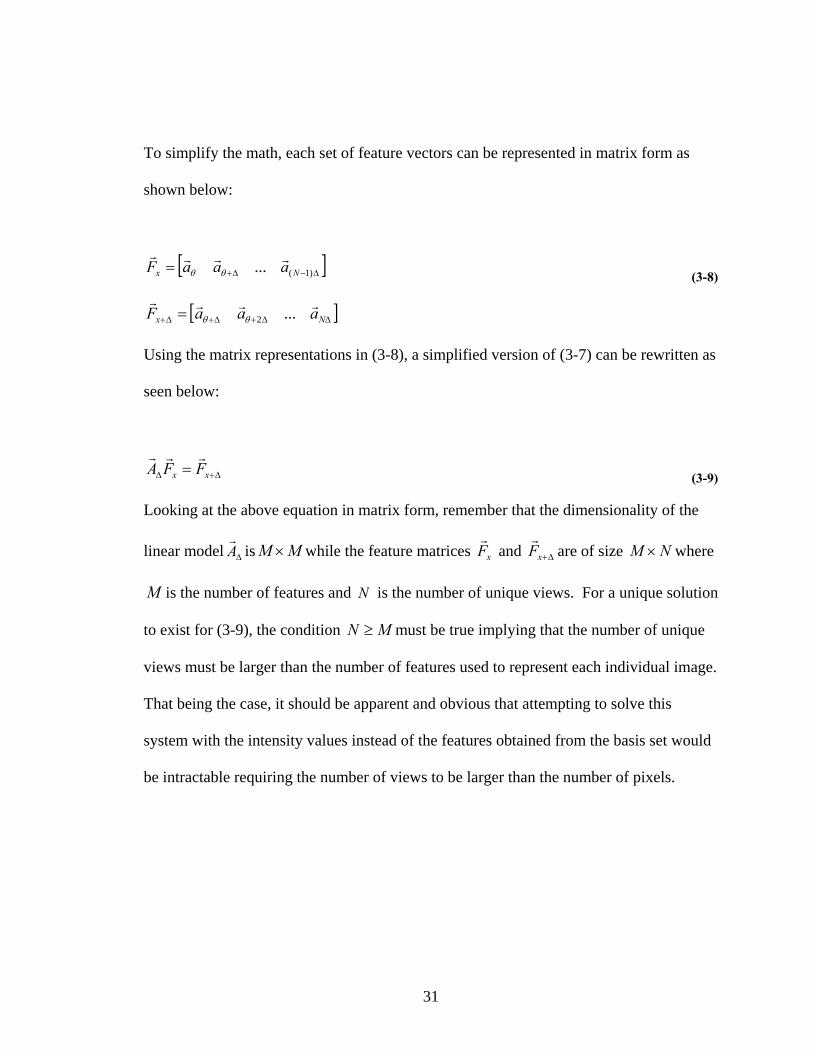
30

To simplify the math, each set of feature vectors can be represented in matrix form as

shown below:

[ ]Δ−Δ+= )1(... Nx aaaF rrrrθθ

(3-8)

[ ]ΔΔ+Δ+Δ+ = Nx aaaF rrrr...2θθ

Using the matrix representations in (3-8), a simplified version of (3-7) can be rewritten as

seen below:

Δ+Δ = xx FFArrr

(3-9)

Looking at the above equation in matrix form, remember that the dimensionality of the

linear model ΔAr

is MM × while the feature matrices xFr

and Δ+xFr

are of size where NM ×

M is the number of features and is the number of unique views. For a unique solution

to exist for

N

(3-9), the condition must be true implying that the number of unique

views must be larger than the number of features used to represent each individual image.

That being the case, it should be apparent and obvious that attempting to solve this

system with the intensity values instead of the features obtained from the basis set would

be intractable requiring the number of views to be larger than the number of pixels.

MN ≥

31

Therefore, by using the features to represent the image, we anticipate that

is satisfied so that the system may be solved. The minimum mean square error

solution for the linear model

MN ≥

ΔAr

is given by:

1)( −Δ+Δ =

Txx

Txx FFFFA

rrrrr (3-10)

Novel Views Prediction

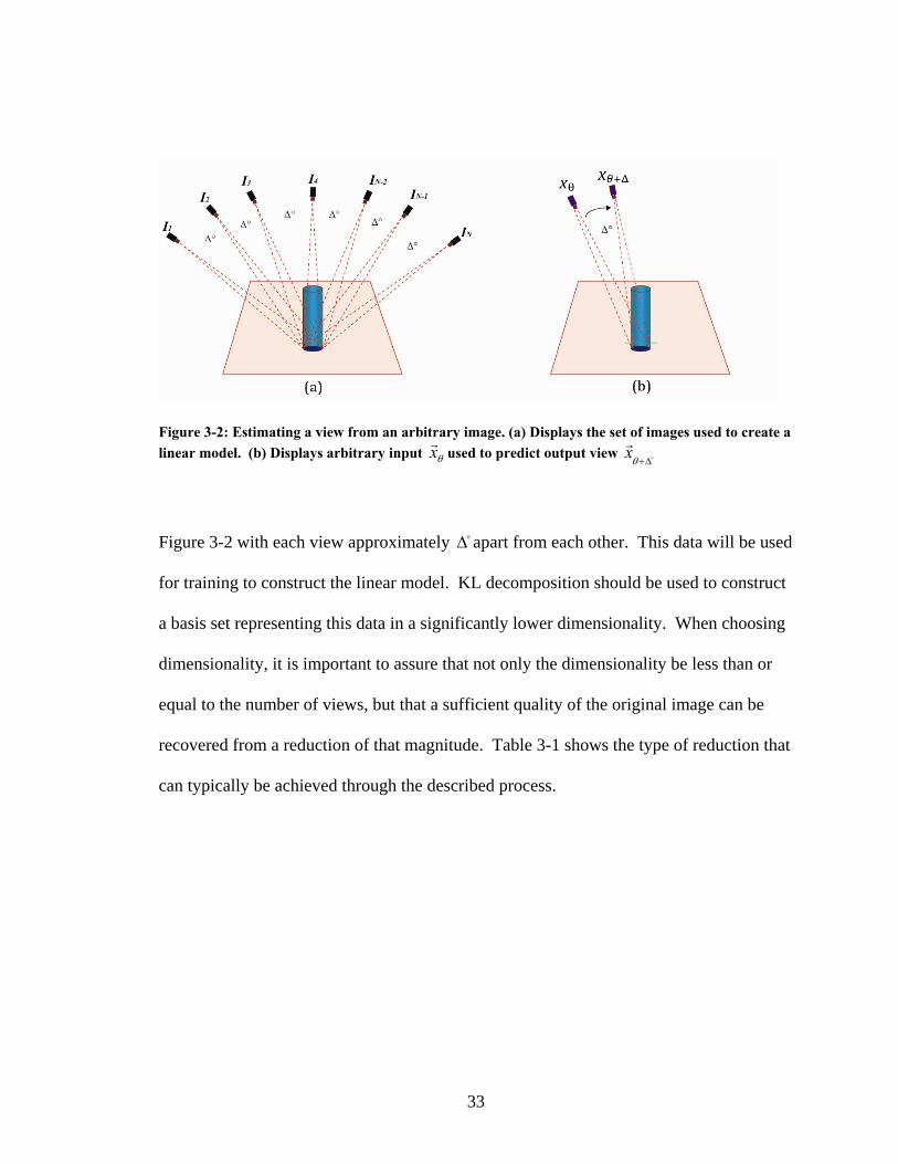
Given a limited amount of two dimensional data from views of an object, consider

the problem of estimating new views of the object while maintaining rigidness in a three

dimensional space. Figure 3-2 helps visualize the problem showing both the set of data

as well as predicting a novel view. Although this problem has been previously solved by

Seitz et al. [1] as mentioned earlier, in certain situations (covered more thoroughly in the

following sections) the view morphing algorithm will either be impractical to use or will

not work. One of the goals of the proposed view synthesis algorithm is to work under

such conditions where conventional view morphing is unlikely to succeed.

In order to predict views using this procedure there are two major steps required,

where the first is to construct a linear model. This is fairly straight forward using the

technique described in the previous section. Specifically, the data should be arranged as

in

32

Figure 3-2: Estimating a view from an arbitrary image. (a) Displays the set of images used to create a linear model. (b) Displays arbitrary input θxr used to predict output view o

rΔ+θ

x

Figure 3-2 with each view approximately oΔ apart from each other. This data will be used

for training to construct the linear model. KL decomposition should be used to construct

a basis set representing this data in a significantly lower dimensionality. When choosing

dimensionality, it is important to assure that not only the dimensionality be less than or

equal to the number of views, but that a sufficient quality of the original image can be

recovered from a reduction of that magnitude. Table 3-1 shows the type of reduction that

can typically be achieved through the described process.

33

Table 3-1: Comparison of model with principle component reduction vs. no reduction

Image Resolution Number of Pixels Required Views (no reduction)

≈Required Views2 (with reduction)

80 x 60 4800 4800 6160 x 120 19200 19200 9320 x 240 76800 76800 13640 x 480 307200 307200 18

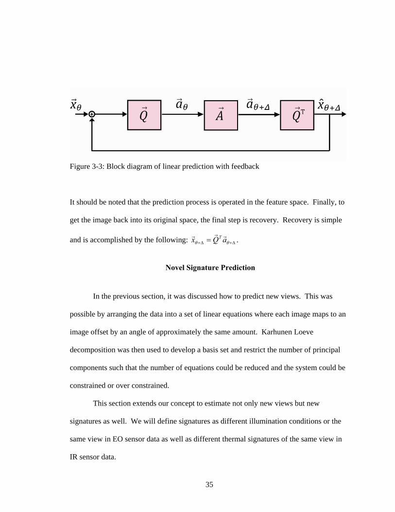
With the basis set solved for and the features extracted, a system of equations can

be established as in the mathematical formulation which can be used to solve for the

linear model. Once the linear model is created it is very simple to estimate a view

apart from any arbitrary view which is the second step. This is observed in oΔ Figure 3-3

which shows a block diagram that takes an input and yields an estimate of that input

rotated by . Additionally, in the figure we observe that that the prediction can be fed

back into the input to generate an estimate of the input rotated by

oΔ

oΔ2 .

2 The amount of required views were solved for experimentally by compressing an arbitrary number of images of the given resolutions using PCA, and observing the average minimum principle components needed to retain an acceptable representation of the original image.

34

Figure 3-3: Block diagram of linear prediction with feedback

It should be noted that the prediction process is operated in the feature space. Finally, to

get the image back into its original space, the final step is recovery. Recovery is simple

and is accomplished by the following: Δ+Δ+ = θθ aQx T rrr .

Novel Signature Prediction

In the previous section, it was discussed how to predict new views. This was

possible by arranging the data into a set of linear equations where each image maps to an

image offset by an angle of approximately the same amount. Karhunen Loeve

decomposition was then used to develop a basis set and restrict the number of principal

components such that the number of equations could be reduced and the system could be

constrained or over constrained.

This section extends our concept to estimate not only new views but new

signatures as well. We will define signatures as different illumination conditions or the

same view in EO sensor data as well as different thermal signatures of the same view in

IR sensor data.

35

Figure 3-4 shows an example of what different signatures of the same object at the same

view can look like. From these examples it is not difficult to visualize that even if

training data exists in a specific object at a specific view, different signatures can make

object recognition a challenge. This being the case, it is an interesting problem to predict

different views of an object, given a new signature.

The process for predicting a new signature is very similar to that of predicting a

new view with the only difference existing in the creation of the linear model. In order to

adequately describe this process a new convention must be established that accounts for

signatures. Let the number of apostrophes indicate a signature identifier with a total of

signatures in the example. All other notations used will be as described previously.

Below we will modify the system described in

3

(3-9) to be a more generalized form

allowing for a linear model that supports multiple signatures.

36

Figure 3-4: Comparison of thermal signatures. The columns show 3 different views while the rows represent different thermal states. This figure is intended to illustrate how different the same object at the same view can look from different thermal states.

⎥⎥⎥⎥⎥⎥⎥⎥

⎦

⎤

⎢⎢⎢⎢⎢⎢⎢⎢

⎣

⎡

=

⎥⎥⎥⎥⎥⎥⎥⎥

⎦

⎤

⎢⎢⎢⎢⎢⎢⎢⎢

⎣

⎡

ΔΔ+Δ+

ΔΔ+Δ+

ΔΔ+Δ+

ΔΔ+Δ+

ΔΔ+Δ+

ΔΔ+Δ+

PM

PPPP

M

M

PM

PPPP

M

M

bbbbb

bbbbbbbbbb

aaaaa

aaaaaaaaaa

A

'''.''''''...........''''''''''''.''.''''

'''.''''''...........''''''''''''.''.''''

*

1111

221

21

21

21

111

11

11

11

1111

221

21

21

21

111

11

11

11

r

(3-11)

The process for creating the general linear predictor that simultaneously handles

multiple signatures and views is very similar to the approach described. Once the linear

predictor has been solved for which supports multiple signature prediction, it can be used

in the same way that the single signature prediction was employed. Figure 3-2 shows the

views used to create the linear model, and how an arbitrary view is used to predict a new

view. Including both signatures and aspect in the estimation process improves (reduces)

the condition number of the matrix and leads to a more numerically stable solution.

37

Sources of Data Degradation

Previous methods in one way or another are heavily dependent on geometric

transformations and perspective principles. In order to adequately achieve this one of the

most basic steps is to establish precise correspondence between training images. This is

typically done by using a feature point extraction method such as Harris corners [12] or

SIFT interest points [11]. Following initial correspondence RANSAC [13] is typically

used to remove any outliers and leave the most likely points corresponding in the training

images. This correspondence can then be used to solve the fundamental matrix from

which geometric transformation will depend on.

This potentially creates a problem because in order to make convincing geometric

transformations, the correspondence must be very precise. This can be difficult

depending on that sensor that captured the data, noise present, and several other concerns.

The remainder of this chapter will discuss these concerns describing when it would be

useful to use an approach to view synthesis that does not depend on establishing

correspondence.

38

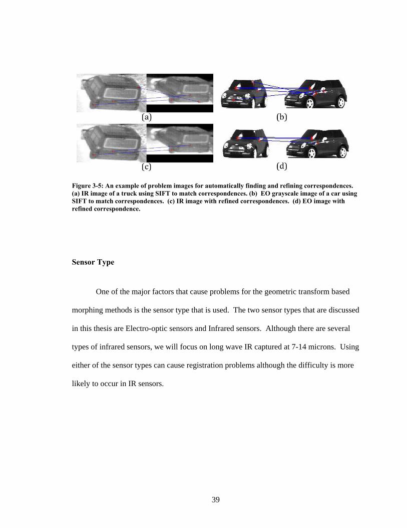
Figure 3-5: An example of problem images for automatically finding and refining correspondences. (a) IR image of a truck using SIFT to match correspondences. (b) EO grayscale image of a car using SIFT to match correspondences. (c) IR image with refined correspondences. (d) EO image with refined correspondence.

Sensor Type

One of the major factors that cause problems for the geometric transform based

morphing methods is the sensor type that is used. The two sensor types that are discussed

in this thesis are Electro-optic sensors and Infrared sensors. Although there are several

types of infrared sensors, we will focus on long wave IR captured at 7-14 microns. Using

either of the sensor types can cause registration problems although the difficulty is more

likely to occur in IR sensors.

39

SNR: Its Affect on Synthesis

In this section, we will focus on noisy data and low contrast data. It is important

to understand the limitations of the data to use the best algorithm for the job. Figure 3-5

shows an example of two problem images which have difficulty finding correspondences.

There are less than 8 correspondences found which is essential for most standard

algorithms such as Hartley et al [14] to compute the fundamental matrix. In order to

achieve good geometric transformations, no false positives can be introduced in

correspondences, and it is difficult to precisely select additional points by manual

techniques.

Noisy Data

While there are many ways to reduce noise in the data, it is not always convenient

to do so. There are several factors that could leave data obtained from both visible and

infrared sensors susceptible to noise. One of the most likely candidates for causing noise

is having a high exposure index, or simply a legacy digital camera shot without the

proper lighting. Of course any digital camera could have noise due to electrical

interference.

40

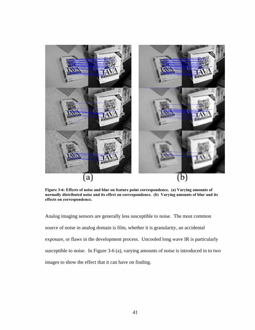
Figure 3-6: Effects of noise and blur on feature point correspondence. (a) Varying amounts of normally distributed noise and its effect on correspondence. (b) Varying amounts of blur and its effects on correspondence.

Analog imaging sensors are generally less susceptible to noise. The most common

source of noise in analog domain is film, whether it is granularity, an accidental

exposure, or flaws in the development process. Uncooled long wave IR is particularly

susceptible to noise. In Figure 3-6 (a), varying amounts of noise is introduced in to two

images to show the effect that it can have on finding.

41

Low Contrast or Blurred Data

Aside from noise, the blur effect (or low contrast) can also be a problem for image

processing. It can have an effect similar to low pass filtering an image, which makes it

more difficult to precisely identify edges and other high frequency characteristics in

images. There are many factors that introduce blur in images. In electro-optic sensors,

factors such as poor focus, camera shake, and motion blur can all create this type of effect

In infrared sensors most accept for upper end sensors cannot come close to matching the

contrast offered in electro-optic sensors. Similarly to noise present in images, Figure 3-6

(b) illustrates the difficulty in finding correspondence with varying amount of blur in the

images.

42

CHAPTER FOUR: EXPERIMENTS & RESULTS

In order to demonstrate the benefits and affects of the proposed algorithm, several

experiments were carried out using multiple datasets. Standard datasets as well as

controlled datasets collected in the lab are represented. Experiments were designed to

test the functionality of the algorithm on normal data as well as data corrupted by noise

and blur. It was also desired to see how varying parameters of the algorithm would affect

the learning of the predictor as well as the output of the algorithm. In addition to analysis

that test prediction quality, we will attempt to show that synthesis can be used to improve

the performance of ATR algorithms. The following section will describe the datasets

used throughout this thesis.

Datasets

Two main datasets were used for the majority of the experiments discussed in this

thesis. You can see a subset of the data used for the experiments in Figure 4-1. It was

important to have a controlled dataset which could show an object of interest from every

possible view for 360 degrees, and hence one of the datasets was collected in the lab.

One of the benefits of a controlled dataset is that ground truth is available for every

possible experiment, and multiple illumination conditions are available which would not

be otherwise.

43

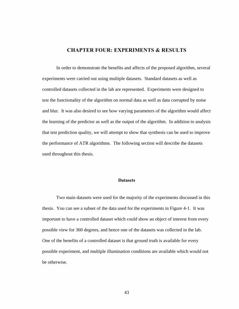
Figure 4-1: Subsets of the major datasets used in this thesis. (a) Sample of the dataset which was collected in lab. (b) Sample of the well known COIL – 100 dataset. (c) Sample of IR data collected

Additionally, it is important to show results from a standard database that is

publicly available. The COIL – 100 dataset [6] was chosen for this purpose. It is

convenient to use for synthesis because it is comprised of 100 objects divided into

categories where each object is shown from 72 different views each having 5 degrees of

separation between the views. The only characteristic about the COIL-100 dataset that

makes it less than ideal is that the scale of the object varies as the view changes.

Unfortunately, this limits the amount of images suitable for our experiments.

Additionally, this dataset was used because other view synthesis and morphing

publications have used the dataset such as Xiao et al [18].

44

Experiments

Varying the Number of Basis Vectors Used to Create the Predictor

The purpose of this experiment is to show the affect on prediction quality as a

function of the number of basis vectors used to estimate the predictor. The measure of

prediction quality is observed by minimizing the mean squared error and maximizing the

correlation between the predicted output and the ground truth. Consider equation (3-10),

where the predictor matrix A is a set of coefficients that will predict the principle

component features corresponding to the appearance of the input rotated by a constant

offset . The number of coefficients in the predictor matrix that need to be estimated is

dependent on the number of principle component features chosen to represent the images.

This relationship between the number of principle components chosen and the number of

coefficients in the predictor is exponential such that if principle components were

chosen, the predictor would be of size . Intuitively this should imply that since the

number of coefficients grow exponentially with the number of principle components

chosen, the error in each predicted coefficient should also grow exponentially. This

would imply that while choosing too few principle component features might not

adequately retain enough of the image to represent it (resulting in poor prediction and

appearing heavily smoothed), choosing too many principle component features could

cause the error grow exponentially with each coefficient resulting in a noisy prediction.

Δ

n

2n

45

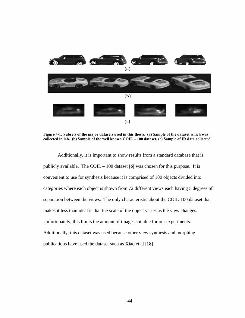
Figure 4-2: Results from experiment 1. (a) Input image. (b) Ideal output image. (c) Predicted output image using the amount of basis vectors that produced the lowest mean squared error. (d) Predicted output image using the amount of basis vectors producing the highest mean squared error. (g) Plot of the mean squared error as a function of the percentage of available basis vectors used.

To test this intuition we have chosen an experiment that learns multiple views as

well as several illumination conditions. This experiment will vary the number of

principle component features used to estimate the predictor. Due to the constraints

established in CHAPTER THREE the upper limit for the number of potential principle

component features is restricted to the number of views multiplied by the number of

signature types or in this case, illumination conditions. Figure 4-2 shows the results of

this experiment described in this section. Observing the results clearly substantiates the

hypothesis that using too few or too many features both result in poor predictions.

46

Figure 4-3: Results from experiment 2. Column 1 is the input, column 2 is the ideal output, and column 3 is the predicted output. (a) Experiment performed with no corruption. (b) Experiment performed with zero mean and standard deviation of 15 white noise corrupting data. (c) Experiment performed with zero mean and standard deviation of 30 white noise corrupting data. (d) Experiment performed with Gaussian blur with radius of 3 corrupting data. (e) Experiment performed with Gaussian blur with radius of 6 corrupting data.

Prediction Quality as a Function of Added Noise and Blur

As suggested in previous chapters, one of the primary benefits of using this

approach to view-synthesis as compared to previous approaches is in the case of blurry

data, noisy data, or data with poor contrast. For this reason it was believed prudent to

have an example that could show prediction quality as a function of data corrupted by

motion and blur. It should be kept in mind that images with large amounts of this type of

corruption cannot have correspondence found by standard methods, making it very

47

difficult or in some cases impossible to use traditional morphing and synthesis

approaches. In this experiment, 4 different synthesis’ were performed which included an

experiment on data with no corruption, corruption by noise, corruption by blur, and

corruption by both noise and blur. The results of this experiment can be seen below in

Figure 4-3.

Predicting Views from a New Signature Type

Many computer vision applications use object recognition to compare a new

object to some sort of training data in order to classify it for some purpose. In these types

of applications, even when a substantial training database exists, it is difficult to

adequately capture all possible variations of the object. Changes in signature type for

example could alter the appearance of the object in such a way to make it difficult to

compare to training data. Of course by signature types this is referring to changes in

illumination in visible and changes in thermal state in infrared.

This experiment is designed to test that the proposed algorithm could effectively

learn a model for an object representing its appearance from multiple signatures.

Furthermore we will demonstrate that using this learned model, we can predict the

appearance of this object from a new signature not present in training data from multiple

views.

For this experiment we use data of the same object from many separate thermal

states and used them as training data. We then introduce a new thermal state no in

48

training and try to predict views from this new thermal state. The setup of the experiment

was fairly simple using the training data to construct a basis set. Then, by following

equations described in previous chapters such as (3-11) an estimate of the predictor is

made. With the predictor solved for, any view of the object from the new thermal state

can be used as input to estimate views from this new illumination condition. Figure 4-4

shows the results for predicting 2 different views. You can see in the predicted outputs

that hot spots match for same location as in the ideal output.

Figure 4-4: Results from experiment 3. In each of the two results a view is predicted from a new thermal state. The left column is the input image, the center column is the ideal image, and the right column is the predicted image. (a) Example 1 input is 80 degrees with a predicted output of 20 degrees. (b) Example 2 input is 135 degrees with a predicted output of 75 degrees.

49

CHAPTER FIVE: CONCLUSION

Summary

This thesis has introduced a novel approach to view synthesis using linear

prediction techniques to estimate the features that represent a synthesized view. We have

shown how to use this algorithm to estimate the appearance of new views for an object.

Additionally, we have shown how to estimate views of an object in new illumination

conditions for visible data and new thermal states for infrared data. All of the constraints

are well described indicating when it would be appropriate to use this algorithm for view

synthesis and when it a more traditional approach may be better suited.

In addition to introducing this novel approach and showing results for its

synthesis, this thesis also demonstrates how a linear prediction technique can be used to

improve the performance of ATR applications. A correlation based approach as well as a

machine learning based approach both realized a boost in performance using the

proposed algorithm to synthesize images that were not adequately represented by training

data.

While the proposed method for view synthesis is not the only method available,

there are several cases where it makes sense to use this approach. It has been well

documented that most previous approaches require a solution for the epipolar geometry

between the reference images which in turn requires an accurate correspondence between

the reference images before it can synthesize new views. We have demonstrated that

50

when noise, blur, and other corruptions are introduced into data, it is difficult to find

accurate correspondences. Additionally, we have shown the difficulties in finding

accurate correspondences in the case of most long wave infrared data. Most algorithms

use a modified version of the 8-point algorithm to obtain the fundamental matrix required

to solve for the epipolar geometry. When the data is corrupted as previously described, it

is difficult to find even a few accurate correspondences let alone the eight accurate

correspondences can be found. In these cases, the proposed algorithm has demonstrated

the ability to synthesize new views and does not depend on correspondences or geometry.

Additionally, new signature types can be estimated. Given that this approach works well

with noisy blurred data and can estimate new signatures, it seems appropriate for use in

the infrared domain where images are commonly low in contrast with some noise present.

In these types of images, a change in the thermal condition can drastically change their

appearance.

Future Work

While the results shown in this thesis are promising, further tests need to assess

the robustness of this approach and its impact on other ATR algorithms. While using

principle components to represent the images in lower dimensions was convenient and

worked well, there may exist a different basis set that could offer better predictions. For

the case where results are to be inputted directly into a machine learning classifier, basis

spaces (that cannot be recovered into their original space or are inconvenient to do so)

51

may be used alternatively. It is also desired to further show improvements in ATR using

the proposed method of View Synthesis. To accomplish this, more time should be spent

collecting appropriatedatasets and setting up scenarios for these experiments.

52

LIST OF REFERENCES

[1] S. Seitz and C. Dyer “View Morphing”, Proceedings of ACM SIGGRAPH 11996,

21-30, 1996

[2] S.E. Chen and L. Wiliams, “View Interpolation for. Image Synthesis,” Proc.

Siggraph 93, ACM Press,. New York, 1993, pp. 279-288

[3] C. Buehler, M. Bosse, L. McMillan, S. Gortler M. Cohen “Unstructured lumigraph

rendering”. in: Proc. ACM SIGGRAPH 2001, 2001, pp. 425–432

[4] McMillan, L., and G. Bishop “Plenoptic Modeling: An Image-Based Rendering

System”, Proceedings of SIGGRAPH 95, (Los Angeles, CA August 6-11, 1995),

pp. 39-46

[5] S. Laveau and O. Faugeras “3-D scene representation as a collection of images” In

Proc. International Conference on Pattern Recognition (1994), 689-691, 1994

[6] S. A. Nene, S. K. Nayar and H. Murase, "Columbia Object Image Library (COIL-

100)," Technical Report CUCS-006-96, February 1996

[7] J. Xiao and M. Shah “Tri-view Morphing”, Special issue of "Computer Vision and

Image Understanding" on Model-based and Image-based 3D Scene Representation

for Interactive Visualization Vol. 96, issue 3 (2004), .345-366, 2004

[8] A. Mahalanobis, B.V.K. Vijaya Kumar, S.R.F. Sims, and J. Epperson,

"Unconstrained Correlation Filters, " Applied Optics , Vol. 33, pp. 3751-3759,

1994

[9] J. Xiao and M. Shah “Two-Frame Wide Baseline Matching”, The Ninth IEEE

International Conference on Computer Vision, Nice, France, 2003

53

[10] K. Mikolajczyk, C. Schmid “An Affine Invariant interest point detector”, Proc.

ECCV, 2002

[11] D. Lowe “Distinctive Image Features from Scale-Invariant Keypoints”, Proc. IJCV

2004

[12] C. Harris and M. Stephens. “A combined corner and edge detector.”, In Alvey

Vision Conference, pages 147-151,1988

[13] M. A. Fischler, R. C. Bolles. “Random Sample Consensus: A Paradigm for Model

Fitting with Applications to Image Analysis and Automated Cartography.”, Comm.

of the ACM, Vol 24, pp 381-395, 1981

[14] R. Hartley, “In Defense of the 8-Point Algorithm”, IEEE Transactions on Pattern

Analysis and Machine Intelligence, 19(2), 133-137, 1997

[15] R. A. Calvo, M. G. Partridge, and M. A. Jabri “A comparative study of principal

component analysis techniques”. In Proc. Ninth Australian Conf. on Neural

Networks, Brisbane, QLD, Feb. 1998

[16] Omar Javed, Khurram Shafique, and Mubarak Shah, "A Hierarchical Approach to

Robust Background Subtraction using Color and Gradient Information", IEEE

Workshop on Motion and Video Computing, Orlando, Dec 5-6 2002.

[17] Omar Javed, Zeeshan Rasheed, Orkun Alatas, and Mubarak Shah, "M-Knight: A

Real Time Surveillance System for Multiple Overlapping and Non-Overlapping

Cameras", Invited paper in IEEE conference on Multimedia and Expo, Special

Session on Multi-Camera Surveillance Systems, Baltimore, July 6-9, 2003.

54

[18] J. Xiao and M. Shah “Automatic Target Recognition Using Multi-View

Morphing”, Conferences of SPIE Automatic Target Recognition XIV, Orlando,

USA, April 13-15, 2004.

[19] Chih-Chung Chang and Chih-Jen Lin “LIBSVM : a library for support vector

machines”, 2001.

[20] S Seitz and C Dyer “Physically-valid view synthesis by image interpolation”,

Workshop on Representations of Visual Scenes, 1995.

[21] S. Seitz, “Image-Based Transformation of viewpoint and scene appearance”,

Dissertation, Computer Science, University of Wisconsin, 1997.

[22] R.I. Hartley, “Theory and practice of projective rectification”, International Journal

of Computer Vision 35 (1999)(2), pp. 115–127

[23] K. Mikolajczyk and C. Schmid, “A performance evaluation of local descriptors”,

Proceedings of IEEE Conference on Computer Vision and Pattern Recognition,

Madison, Wisconsin, USA, 2003.

[24] Q. T. Luong, "Fundamental matrix and self-calibration", PhD Thesis, University of

Paris, Orsay

[25] R. I. Hartley, A. Zisserman, “Multiple View Geometry in Computer Vision”, 2nd

Edition, Cambridge University Press, 2003.

[26] S. M. Seitz, C. R. Dyer, “Complete structure from four point correspondences”, in

Proc. Intl. Conf. on Computer Vision, 1995.

55

[27] John Mallon, Paul F. Whelan, "Projective Rectification from the Fundamental

Matrix", Image and Vision Computing, Volume 23, Issue 7, July 2005, Pages 643-

650

[28] C. Cortes and V. Vapnik, "Support vector networks_ Machine Learning", 20:273-

297, 1995.

[29] Marti A. Hearst, "Support Vector Machines," IEEE Intelligent Systems, vol. 13,

no. 4, pp. 18-28, July/Aug. 1998

[30] P.J. Grother, "Handprinted Forms and Character Database, NIST Special Database

19", NISTIR March 1995

[31] F. Rosenblatt, “The Perceptron: A Probabilistic Model for Information Storage and

Organization in the Brain”, Cornell Aeronautical Laboratory, Psychological

Review, v65, No. 6, pp. 386-408

56