WATER RESOURCES RESEARCH, VOL. 27, NO. 9, PAGES 2401-2414, SEPTEMBER 1991

A Stochastic Analysis of Pumping Tests in Laterally Nonuniform Media

JAMES J. BUTLER, JR. 1

Kansas Geological Survey, University qœ Kansas, Lawrence

Conventional pumping test analysis methodology assumes that aquifer transmissivity is invariant in space. The ramifications of this assumption are examined for hypothetical units whose variations in transmissivity are considered to be reasonable representations of variations possible in natural systems. The dependence of pumping test transmissivity on spatial (angular and radial) and temporal location of observations and the method of drawdown analysis is assessed. The dependence on the angular position of an observation well appears of little significance. Dependence on radial position, however, can be strong. The dependence on the interval of time used in the pumping test analysis is only important in highly variable systems. Methods of drawdown analysis that yield identical estimates in uniform units yield differing estimates in nonuniform ones as a result of a difference in data-fitting procedures. A reasonable estimate of transmissivity at a regional scale can be obtained from a Cooper-Jacob analysis applied at a large duration of pumpage. In general, conventional approaches for pumping test analysis should be viable in the nonuniform aquifers of the type considered here.

INTRODUCTION

A pumping test is the primary means of assessing the transmissive and storage properties of subsurface material c•n a scale of significance for issues involving water supply or the gross movement of a contaminant plume. The parame- ters characterizing the transmissive and storage nature of a unit are estimated from pumping-induced drawdown using a•ytical solutions to the partial differential equation gov- erning the flow of groundwater to a central pumping well. These analytical solutions assume that the aquifer is uniform or can be subdivided into, at most, two or three uniform regions [Streltsova, 1988]. Although most hydrogeologists recognize that natural systems are characterized by a con- siderable degree of spatial variability, only limited work has been done to evaluate the ramifications of that variability for pumping test analyses [e.g., Warren and Price, ! 961; Van- denberg, 1977]. This article describes an attempt to address these ramifications in more depth than previous work.

The major purpose of the work reported here is to examine theoretically the applicability of conventional pumping test an/'•ysis methodology, developed for uniform units, to units ',•hose properties vary in space. Specifically, this examina- tion focuses on the impact of lateral variations in the transmissive properties of a unit on the transmissivity esti- mates obtained from conventional pumping test analysis raethodotogy. The impact of these lateral variations is quan- tified using the dependence of the estimated transmissivity •n The spatial and temporal location of the drawdown data employed in the analysis (in this work spatial location refers t:0 position of the observation well, and temporal location refers to the interval of time represented by the drawdown da•.a). Only behavior in perfectly confined aquifers is con- :s'dered here. This simplification allows the effect of lateral ¾mations in transmissivity to be more readily evaluated. !•he emphasis of this study is on conditions in units that

•are representative of those that might be found in natural

• Formerly at the Department of Applied Earth Sciences, Stanford Ut•.iver.sity, Stanford, California.

Copyright !99! by the American Geophysical Union. l•aPer n 'tan•r 91WR01371. 00t•. ! '397/91/91WR-0137 ! $05.00

systems. Thus an effort is made to employ mathematical representations of units whose spatial variations in transmis- sivity can be considered to be reasonably similar to those of aquifers in the field. Since detailed deterministic descriptions of variations in transmissivity over a field area are not available, a stochastic process representation is employed to incorporate the limited existing field data into this study. An important advantage of a stochastic representation is that it allows the uncertainty concerning the actual spatial varia- tions in natural systems to be incorporated into the analysis. The results of this work are therefore phrased in terms of behavior in the class of units that can be represented by a specific stochastic process.

Since conventional pumping test analysis methodology is often used to provide estimates of the regional properties of a flow system, this work also examines the viability of the transmissivity calculated from a pumping test analysis for use in a regional flow model. The aim of this aspect of the work is to define appropriate procedures for estimation of the regional transmissivity from drawdown data collected during a pumping test.

METHODOLOGY

The basic approach of this research is to numerically simulate a pumping test in a realization drawn from a stochastic process characterizing the variations in transmis- sivity over the modeled area. A pumping test transmissivity is then estimated from the simulated drawdown data using conventional analytical approaches. The dependence of the estimated transmissivity on the spatial and temporal location of observations, and the method of drawdown analysis (the various forms of transmissivity dependence are henceforth denoted as dependence relationships), is then calculated for that realization. Monte Carlo simulation is employed to repeat this procedure over a sample of realizations drawn from the stochastic process. The average and variability of the dependence relationships over the realizations drawn from the stochastic process are then used to assess the viability of conventional pumping test analysis methodology in the class of units represented by that process. Four stochastic processes are examined in the work discussed here. Given the large computational demands of Monte

2401

2402 BUTLER: A STOCHASTIC ANALYSIS OF PUMPING TESTS

Carlo simulation, the emphasis of this study will be on obtaining a general understanding of these dependence rela- tionships, rather than the definition of highly precise expres- sions describing their form.

A finite element model, the FE3DGW model of Gupta et al. [1984], is employed for the simulations of this work. Equation (1) is the form of the flow equation used here:

•+---+ T --S-- + r Or 2 r Or • •-• (1)

where

T transmissivity, equal to/•B, L2/T; S storage coefficient, equal to So B, dimensionless; ? integrated vertical average of drawdown, L; B aquifer thickness, L;

K, So integrated vertical average of hydraulic conductivity and specific storage, respectively;

r radial direction, L; 0 angular direction, rad.

The initial and boundary conditions used in the simulations are

?(r, 0, 0)=0 rw<r<r b 0-< 0-<2,r (2a)

?(r b, 0, t) = 0 0 <-- 0 --< 2,r t > 0 (2b)

rwr dO = -Q t > 0 (2c)

where Q is the pumpage from the central well, L3/T; r w is the radius of the pumping well, L' and rb is the radius of the outer aquifer boundary, L.

For the simulations of this work a pumping well with a radius of 0.07 m, an outer aquifer boundary that is 1930 m from the pumping well, and a pumpage rate of 6250 m3/d are employed. The finite element grid, which consists of quad- rilateral elements, utilizes an equal log spacing in the radial direction, with approximately four elements per log cycle. Sixteen elements are employed in the angular direction. A pumping period of 2.7 days is used in the majority of the simulations, a duration considered adequate to represent conditions faced in many pumping tests. One set of simula- tions is carried out for a significantly longer duration (43.25 days) in order to evaluate behavior at very large times. In neither case does the constant head boundary at 1930 m significantly influence the observation well drawdown.

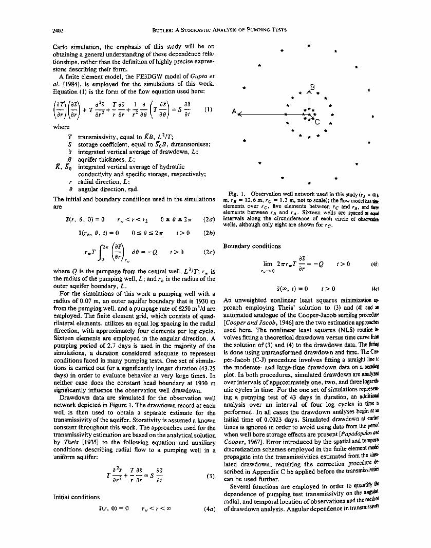
Drawdown data are simulated for the observation well network depicted in Figure 1. The drawdown record at each well is then used to obtain a separate estimate for the transmissivity of the aquifer, Storativity is assumed a known constant throughout this work. The approaches used for the transmissivity estimation are based on the analytical solution by Theis [1935] to the following equation and auxiliary conditions describing radial flow to a pumping well in a uniform aquifer:

O 2? T O• To7+ = S -- (3) r Or Ot

Initial conditions

•(r, 0) = 0 r•. < r < m (4a)

Fig. 1. Observation well network used in this study (rA = 49,• m, re = 12.6 m, rc = 1.3 m, not to scale); the flow model has ..'me elements over r c, five elements between r c and re, and three elements between r e and r A. Sixteen wells are spaced at • intervals along the circumference of each circle of observatim wells, although only eight are shown for r c.

Boundary conditions

0•

lim 2Z'rwT • = -Q r,,,--> 0 Or

t > 0

•(m, t)=o t>o

An unweighted nonlinear least squares minimization a½ proach employing Theis' solution to (3)and (4} and '• automated analogue of the Cooper-Jacob semilog procedure [Cooper and Jacob, 1946] are the two estimation approac• used here. The nonlinear least squares (NLS) routine i•, volves fitting a theoretical drawdown versus time curve fro• the solution of (3) and (4) to the drawdown data. The is done using untransformed drawdown and time. The Coo- per-Jacob (C-J) procedure involves fitting a straight line • the moderate- and large-time drawdown data on a plot. In both procedures, simulated drawdown are analyze• over intervals of approximately one, two, and three logamY mic cycles in time. For the one set of simulations represe•' ing a pumping test of 43 days in duration, an additional analysis over an interval of four log cycles in time performed. In all cases the drawdown analyses begin at • initial time of 0.0023 days. Simulated drawdown at earlier times is ignored in order to avoid using data from the pem• when well bore storage effects are present [Papa&•pulos an Cooper, !967]. Error introduced by the spatial and tempor• discretization schemes employed in the finite element model propagate into the transmissivities estimated from the simu lated drawdown, requiring the correction procedure scribed in Appendix C be applied before the transmissivitie:• can be used further.

Several functions are employed in order to quantify t• dependence of pumping test transmissivity on the angu radial, and temporal location of observations and the met• of drawdown analysis. Angular dependence in tran.s rnissiv•

BUTLER: A STOCHASTIC ANALYSIS OF PUMPING TESTS 2403

values is assessed using a coefficient of variation and the •xmMized absolute value of the transmissivity difference.

•is coefficient of variation consists of the standard devia- tion of transmissivity values calculated at individual wells about the circumference of a circle of observation wells (see F:•are 1) over the mean of these values. The normalized .•erence consists of the absolute difference between trans- mssivity values calculated at two wells spaced at a given •ar separation normalized by the value at the first well. Both wells are at the same radial distance from the pumping •vell. In this paper the coefficient of variation is primarily employed for describing the angular dependence, since it ;more succinctly summarizes the studied relationships. Note :•at the observation well network displayed in Figure 1 results in drawdown being measured at equal angular inter- vals at different radial distances from the pumping well. :•easurement at equal angular intervals produces sampling schemes that are not strictly comparable from one circle of observation wells to the next, because the sampling interval relative to the correlation structure of the stochastic process •:reases with radial distance from the pumping well. Given the goals of this work, however, the differences between •ampling schemes are considered insignificant.

Rad'ml and temporal dependence are characterized by the mmalized absolute value of the transmissivity difference. h each case a transmissivity value calculated from draw- rtown at the pumping well is considered the base value for the realization, The absolute value of the difference between

dis base value and a transmissivity computed at a different ,radi;al or temporal location is normalized by the base value. I1• normalized absolute value of the transmissivity differ- ence is also used to characterize parameter dependence on

t• method of drawdown analysis, with the NLS transmis- •vity being used as the normalizing value for the difference between the NLS and C-J parameters.

The mean and standard deviation of these functions over a

stochastic process are the quantities of interest in this work. !n order to estimate these statistics, the procedure of pump- •,'• test simulation and drawdown analysis is repeated for a :sample of realizations drawn from a given stochastic pro- ½ess. The TUBA program [Mantoglou and Wilson, !98!], •hich implements a two-dimensional form of the turning bands method of Matheron [ 1973], is used for the generation

of realizations of spatially correlated transmissivity values. T• TUBA program generates rectangular elements in a 'Cartesian grid system. As is described in Appendix A, the

Cartesian coordinate output from the TUBA program is transformed into the polar coordinate grid system used in the pumping test simulations. A stratified sampling scheme &scribed in Appendix A is employed to reduce the number of reflizations required for the repetitive Monte Carlo sim- '•lation. A stratified sample of twenty realizations is used in all but one of the cases examined here. This sampling procedure is considered appropriate, given the earlier-stated emesis of this work on general understanding rather than •,ed description. The stochastic processes employed in this work are based

m the Quadra Sands data of Smith [ 1978]. As is described in .•4•pendix B, the core-scale data of Srnith[ 1978] are regular- 'm•d to the scale of a block 10 m by 10 m in lateral extent in On•r to reduce the computational demands of the realiza- L•'•on-•.r}eration procedure. The stochastic process defined by the regu!arized Quadra Sands data is then modified by

TABLE 1. Stochastic Processes Employed in This Work

Case Number Process

1 E{Y} = -3.32 •4r) = 0.04537•I - e

2 E{Y} = -3.32 •4r) = 0.04537(i - e

3 ElY} = -3.32 •(r) = 0.1589(1 - e

4 E{Y} = -3.32 •r) = 0.3452(1 - e

E{ } is the expected value operator; Y = In /•, /• (hydraulic conductivity averaged over a 10 by 10 by 30 m (xyc) block) is measured in centimeters per second; and •r) is the semivariogram value for separation distance r(see (B1) and (B4)of Appendix B for further details). Since all the stochastic processes are Gaussian, isotropic, and second-order stationary, the expected value and semivariogram expressions given for each case are sufficient to fully describe that process. A double-exponential semivariogram model is employed for all cases in order to allow the greater continuity at the origin produced by regularization to be included in the analysis.

decreasing the distance over which values are correlated and increasing the variance in order to allow behavior under conditions of greater variability to be assessed. These mod- ifications are based on geologic considerations and a litera- ture review of existing laboratory and field data. Table 1 lists the Quadra Sands-based stochastic process (case !) and the modifications used in this work. The stochastic processes of Table 1 are written in terms of the hydraulic conductivity averaged over the block. Given the aquifer thickness of 30 m used here, this translates into an expected value for trans- missivity between 959 and 1114 m2/d for the four cases examined in this work. The span of conditions represented by these four cases allows pumping test behavior in laterally nonuniform units to be assessed over conditions that might be met in the field. Further details concerning these cases and the motivation for their selection can be found in

Appendix B. Note that a constant storativity of 0.0795 is used throughout this work.

RESULTS

Dependence on Angular Location

The dependence of pumping test transmissivity on the angular location of observation wells is the first issue to be examined. Figure 2 is a dimensionless plot for the results of an analysis using the first stochastic process (case 1) of Table 1. This graph depicts the mean coefficient of variation as a function of the normalized distance from the pumping well to the ring of observation wells. Throughout this work, the distance between the pumping and observation wells is normalized by the range of the semivariogram of the sto- chastic process. This normalization is used only to relate the observation well location to the correlation structure of the

stochastic process and does not indicate that the results are independent of the specific semivariogram range used in the analysis. Note that the confidence intervals shown on Figure 2 and following figures are approximate 95% confidence intervals calculated assuming a finite sample drawn from a normal distribution of an unknown mean and variance,

Figure 2 clearly shows that the coefficient of variation increases with distance from the pumping well. This rela- tionship is seen in all the cases examined here, and it

2404 BUTLER: A STOCHASTIC ANALYSIS OF PUMPING TESTS

1

1 0 -• 1 0 -2 1 0 -• DISTANCE (DIMENSIONLESS)

Fig. 2. Mean coefficient of variation versus distance plot for case 1 of Table 1 (distance normalized by semivariogram range); duration of analysis is three log cycles in time.

14-

o12 o

10

z

8

6

CASE THREE 4

2 CASE TWO

, , ,,i , 1, , , 0.001 0.01 0.1 1

DISTANCE (DIMENSIONLESS)

CASE FOUR

Fig. 3. Mean coefficient of variation versus distance plot for cases 2-4 of Table 1 (distance normalized by semivariogram duration of analysis is three log cycles in time.

essentially reflects the greater variability in transmissivity that is being met about the circumference of the ring of observation wells as this circumference increases in size.

Note that the pumping test transmissivity values employed in the analysis of angular and radial dependence are deter- mined using the NLS procedure. The C-J procedure is only used for the analysis of temporal dependence, as is explained shortly.

Figure 3 summarizes the results of the analysis of angular dependence for cases 2-4 of Table 1. Clearly, as the variance of the stochastic process increases, the mean coefficient of variation also increases. These increases in the coefficient of

variation are expected, as greater variability is being met over the same separation distance. The Monte Carlo simu- lation for case 3 is carried out for thirty realizations. Table 2 details how the statistics change with the number of realiza- tions. The magnitude of Sc• relative to CV demonstrates that the number of realizations employed in this study is reasonable, given the previously stated goals of this work. Note that the relative magnitude of S cv indicates that, although the estimate of the mean might be acceptable, there may be considerable uncertainty concerning the applicability of this mean value to characterize behavior in any single realization.

For case 4 of Table 1 a ring of observation wells is als0 placed at a distance of 124 m from the pumping well. TI•s additional ring of wells allows behavior at distances of t• order of the range of the semivariogram of the stochast/c process to be examined. As shown in Figure 3, the me.a• coefficient of variation continues to increase through dis- tances close to the range of the stochastic process. Alth0ug not examined further here, such increases in the mea• coefficient of variation with distance would be expected m continue until the portion of the aquifer controlling the response at each observation well reaches a size at which the degree of correlation between volumes of that size begins t• overwhelm the effect of the separation distance. Note tha• the analytical solution described by Butler and Liu [!989: ,• analytical solution for flow to a well in radially asymmet 'r• nonuniform media, submitted to Water Resources Research, !991 (hereinafter J. Butler and W. Liu, submitted manu- script, 1991)] and Butler [1990] for flow in a radially asym- metric nonuniform aquifer can be used to study how the portion of the aquifer controlling the response at an obser- vation well increases with radial distance from the purnpi• well. On the basis of results from a study using that analyt- ical solution (J. Butler and W. Liu, submitted manuscrip• 1991) it is clear that for a circle of observation wells at a large

TABLE 2. Dependence of Monte Carlo Results on the Number of Realizations for Case 3 of Table 1

Radius of Number of

Observation,* m Realizations CVt S cv$ S•'põ

1.3 (0.008) 10 9.91 X 10 -4 6.56 X 10 -4 , 2.07 x 10 -4 20 9.50 x 10-4 5.30 x 10-4 1.19 x 10-4 30 9.75 x 10 -4 4.89 x 10 -4 0.89 x 10 -4

12.6 (0.08) !0 2.35 x 10 -2 1.48 x 10 -2 4.68 x 10 -3 20 2.34 X 10 -2 !.33 X 10 -2 2.97 x 10 -3 30 2.36 x 10 -2 1.20 x 10 -2 2.19 x 10 -3

49.6 (0.3) i0 4.36 x 10 -2 1.33 x 10 -2 4.21 x 10 -3 20 4.52 X !0 -2 1.92 X 10 -2 4.29 x 10 -3 30 4.51 x 10 -2 1.96 x 10 -2 3.58 x 10 -3

*Normalized radius in parenthesis. ?CV is the mean coefficient of variation. $Scv is the standard deviation of the coefficient of variation. õS•-• is the standard deviation of the mean coefficient of variation.

BUTLER: A STOCHASTIC ANALYSIS OF PUMPING TESTS 2405

10

z 2

-' 'i'd -: i'S -' DISTANCE (DIMENSIONLESS)

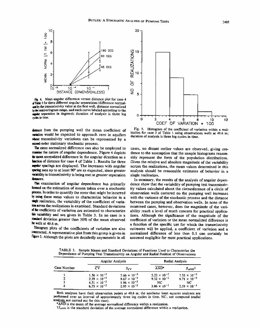
Fig. 4. Mean angular difference versus distance plot for case 4 •f?.able I for three different angular separations (difference normal- • by the transmissivity value at the first well, distance normalized • ,the semivariogram range, and each curve labeled according to the ,•,ar separation in degrees); duration of analysis is three log cycles in time.

2O

I180 DEC; O3 15 Z

//e0 9_O 45 DEG "-i

0 '

•-•e from the pumping well the mean coefficient of -.variation would be expected to approach zero in aquifers •:•se transmissivity variations can be represented by a second-oMer stationary stochastic process.

The mean normalized difference can also be employed to e. * •..x•ne the nature of angular dependence. Figure 4 depicts the mean normalized difference in the angular direction as a '•Mmion of distance for case 4 of Table 1. Results for three

a• •ge!ar spacings are displayed. The increases with angular •ie•g seen up to at least 90 ø are as expected, since greater va•itity in transmissivity is being met at greater separation

This examination of angular dependence has primarily f.•sed on the estimation of means taken over a stochastic process. In order to quantify the error that might be incurred by usiag these mean values to characterize behavior in a ½:• realization, the variability of the coefficient of varia- '".ta• across the realizations is examined. Standard deviations ff the coefficients of variation are estimated to characterize 'Ms variability and are given in Table 3. In no case is a ':•ard deviation greater than 50% of the mean observed for wells at 49.6 m.

Histogram plots of the coefficients of variation are also co•stmcted. A representative plot from this group is given in F•re 5. Although the plots are decidedly asymmetric in all

o

z 5-

0

0 | II I III I •

2 z

,,

i ! I i i

6 1 I'--'--''•i '' I I I l

8 10 12

COEF OF VARIATION ß 100

Fig. 5. Histogram of the coefficient of variation within a real- ization for case 3 of Table 1 using observations wells at 49.6 m; duration of analysis is three log cycles in time.

cases, no distant outlier values are observed, giving cre- dence to the assumption that the sample histograms reason- ably represent the form of the population distributions. Given the relative and absolute magnitude of the variability across the realizations, the mean values determined in this analysis should be reasonable estimates of behavior in a single realization.

In summary, the results of the analysis of angular depen- dence show that the variability of pumping test transmissiv- ity values calculated about the circumference of a circle of observation wells centered on the pumping well increases with the variance of the stochastic process and the distance between the pumping and observation wells. In none of the examined cases, however, does the magnitude of the vari- ability reach a level of much concern for practical applica- tions. Although the significance of the magnitude of the coefficient of variation or the mean normalized difference is a function of the specific use for which the transmissivity estimates will be applied, a coefficient of variation and a normalized difference of less than 0.! can certainly be assumed negligible for most practical applications.

TABLE 3. Sample Means and Standard Deviations of Functions Used to Characterize the Dependence of Pumping Test Transmissivity on Angular and Radial Position of Observations

Angular Analysis Radial Analysis ,,

Case Number C--V Scv •ND* SAND?

1 1.56 x 10 -2 7.66 x 10 -3 2.22 x 10 -2 7.55 x !0 -3 2 2.39 x 10 -2 9.67 X 10 -3 9.32 x 10 -2 6.71 x 10 -2 3 4.51 x 10 -2 !.96 x 10 -2 NC NC 4 6.73 x 10 -2 2.95 x 10 -2 3.06 x 10 -• 2.53 x !0 -l

Both analyses have their observation points at 49.6 m; the nonlinear least squares analyses are performed over an interval of approximately three log cycles in time. NC, not computed {radial anal sz.5•not carried out for this case).

*AND is the mean of the average normalized difference within a realization. ?S,•r• is the standard deviation of the average normalized difference within a realization.

2406 BUTLER: A STOCHASTIC ANALYSIS OF PUMPING TESTS

5O

. 40

m 3o

¸

ZlO

CASE FOUR

- , , , 1,,,, , , , ,,,,, , , , 0

1 o -• 1 o -2 10 -• 1 DISTANCE (DIMENSIONLESS)

Fig. 6. Mean radial difference versus distance plot for cases 2 and 4 of Table 1 (difference normalized by the transmissivity value at the pumping well and distance normalized by the semivariogram range); duration of analysis is three log cycles in time.

Dependence on Radial Location

The dependence of pumping test transmissivity on the radial location of observation wells is the next issue to be examined. As discussed earlier, the normalized absolute value of the difference in transmissivity between that calcu- lated at an observation well and that at the pumping well is the quantity employed to characterize radial dependence. Figure 6 depicts the radial dependence relationships ob- served for cases 2 and 4 of Table 1. The relationships are similar to those illustrated in Figure 3, with increases in the variance of the stochastic process and the distance to the observation well leading to a larger mean difference. Al- though the general form of the relationships is similar to that observed in the angular analysis, the magnitude of the dependence is considerably greater. If, as in the angular analysis, a mean normalized difference of less than 0.1 can be assumed negligible, Figure 6 indicates that the difference between a transmissivity value calculated at the pumping well and one calculated at a distant observation well may be significant in the more variable aquifers. Unlike the angular case, this difference should not decrease to zero at a very large distance from the pumping well. Although not demon- strated here, theoretical considerations indicate that the difference should stabilize near the mean value of the fol-

lowing quantity [see Butler and Liu, 1989, also submitted manuscript, 1991 ]:

T•m

] (5) where Tg m is the geometric mean of the transmissivities employed in the realization, and Tpw is the transmissivity calculated from drawdown at the pumping well. The geomet- ric mean is used in (5) as a surrogate for the value toward which the transmissivity of increasingly larger volumes of the aquifer will converge as a result of the methodology employed in this study, an issue that is discussed further in succeeding pages.

The analysis of radial dependence is incomplete without considering the error that may be introduced when employ- ing an estimate of the mean radial dependence to character-

ize behavior in a single realization. The sample standa-• deviations, employed to quantify the variation in the ized difference across the sampled realizations, are listed ix Table 3. Note that standard deviations greater than 7•,• the mean are calculated for cases 2 and 4. Such large relaiYe values coupled with the magnitude of the estimated imply that there is considerable uncertainty when estirn• behavior in a single realization using the mean relationsh½s• Histogram plots of the absolute normalized difference w'ith• a realization reinforce this point. For case 4 the mean over the sampled realizations is shown to have relatively lirnite• value for characterizing behavior in a single realization w'he• considering observations at 49.6 m (Figure 7, line AI, Tk average difference from one realization indicates that at leaI an order of magnitude change in transmissivity is possible over that separation distance. Although the average norrr,d- ized differences are smaller closer to the pumping (Figure 7, line B) or for a less variable process at the .sa• radial distance (Figure 7, line C), even in these instar•es• differences of over 3 times the mean value are seen. Thus mean values must be used cautiously when characterizir! the radial dependence in any single realization. Note that tk form of the histogram given by line A of Figure 7 indicaief that more realizations would be required in the Monte Carlo simulation to better estimate the nature of the distribution

the average normalized difference in the more variabk cases.

In summary, the results of the above analysis show • for case 4 the issue of radial dependence is of concern for distances greater than about 15 m. For case 2, however, issue of radial dependence is only a concern at much lar•r distances, although considerable variations are possible a distances as small as 50 m. Note that a much greater variability across realizations is seen in the radial analy•s than in the angular. This is due to small areas of anomalous character in the vicinity of the pumping well having

20-

zs- i O ,

I N '

i

la.. .

O Z 5

0 20 40 I'• 80 ,00 AV NORM DIF[ ß 100 Fig. 7. Histograms of the average radial difference

realization for a duration of analysis of three log cycles (difference normalized by the transmissivity value at the well; line A, results for case 4 of Table I using observation 49.6 m; line B, results for case 4 of Table 1 using ob•ervatkm at 12.6 m; and line C, results for case 2 of Table 1 wells at 49.6 m).

BUTLER: A STOCHASTIC ANALYSIS OF PUMPING TESTS 2407

./•.• CASE FOUR ••__• CASE TWO

10' .... i'•)' i'6' ..... i'(• ,o DURATION (DIMENSIONLESS)

Fig. 8. Mean temporal difference versus duration of analysis for cases 2 and 4 of Table 1 (difference normalized by the transmissivity calculated over one log cycle in time and duration normalized as .::&•cussed in text); observation point is the pumping well.

20-

'15'

•1o

o

z 5- z

,,1

:• o• lO

c-J

DURATION (DIMENSIONLESS) Fig. 9. Mean temporal difference versus duration of analysis for

case 4 of Table 1 (difference normalized by the transmissivity calculated over one log cycle in time, duration normalized as discussed in text, and curves labeled according to the method of drawdown analysis); observation point is the pumping well.

ccesWerable influence on the radial dependence as a result of their large impact on drawdown at or near the pumping well. Such small anomalous areas have much less influence

o• drawdown when located near observation wells placed a•ong the circumference of a circle at a distance from the •mping well. This radial dependence in the impact of small areas of anomalous properties on drawdown, which is con- sidered further by Butler and Liu [1989, also submitted manuscript, !991], results in greater variability being seen across the realizations for the radial analysis.

Dependence on Temporal Location

•te issue of temporal dependence can only be partially addressed using the simulation results, owing to discretiza- tion effects propagating into the transmissivity calculations •d producing sizable uncertainties at small dimensionless times, as discussed in Appendix C. Therefore only the temporal dependence at the pumping well is considered :•here. The normalized absolute difference described earlier is employed to characterize temporal variations in transmissiv- ;•ty. In this case the transmissivity calculated over the first bg cycle in time serves as the normalizing quantity.

Figure 8 is a dimensionless plot of the mean normalized absolute transmissivity difference versus the duration of the '•,•ysis. This plot shows that tlae mean difference does not exceed 5% for either case. Thus for observation points near t.he •mping well the calculated transmissivity is essentially L•ependent of the duration over which the analysis is pedbrmed. Note that the analysis is carried out for a larger •aration for case 4, owing to the longer pumping period used h• that case. Note also that the duration of the analysis is •t• as a dimensionless quantity (4Tœvt/Sr2), where TL. v is the expected value of the stochastic process. Up to this point, only pumping test transmissivities calcu-

.'•ted using the nonlinear least squares routine have been ,•oyed. Often, however, the Cooper-Jacob approach is '.•zed for analysis of pumping-induced drawdown. Though •.•se two methods produce identical results in uniform units •1 •.mensionless times greater than 100, the question of their :.•ity in nonuniform units needs to be addressed. This :•'• • equality is evaluated here by comparing results from

the two approaches using drawdown at the pumping well, where dimensionless times are much greater than the sug- gested limiting value of 100.

The temporal dependence of transmissivity values calcu- lated using the NLS and C-J approaches is illustrated in Figure 9 for case 4. Though, clearly, the transmissivities calculated using the C-J approach display a greater temporal dependence, the magnitude of the mean normalized differ- ence does not merit a great deal of concern. An analysis of the variability of the normalized difference across the sam- pled realizations, however, indicates that temporal depen- dence may be important in the C-J case for the more variable aquifers. This is shown by the histogram plot of Figure 10, where normalized differences of greater than 0.30 are ob- served for the C-J estimates. Variability across the sampled realizations is not important for the NLS estimates. Al- though not demonstrated here, theoretical considerations

20-

•15 o

0 6 12 T ! 24 NOMI lOO 30 36

Fig. 10. Histograms of the temporal difference within a realiza- tion for case 4 of Table 1 for a duration of analysis of four log cycles in time (difference normalized by the transmissivity calculated over one log cycle in time: solid line, results for transmissivity calculated using the Cooper-Jacob approach and dashed line, results for transmissivity calculated using the nonlinear least squares ap- proach); observation point is the pumping well.

2408 BUTI.œR: A STOCI•AS'rIC ANALYSIS OF PUMPING TESTS

30-

---- 20

olo z

z

DURATION (DIMENSIONLESS) Fig. !1. Mean difference between transmissivities calculated

using Cooper-Jacob and nonlinear least squares methodologies versus duration of analysis for case 4 of Table 1 (difference normal- ized by the nonlinear least squares transmissivity value and duration normalized as discussed in the text); observation point is the pumping well.

60-

i

_ 40

o 20 z

z

NLS

C-J

10' 10' '{'•)8 'i'6 •" ' 10'ø DURATION (DIMENSIONLESS)

Fig. 12. Mean difference between pumping test transmissivit'es and the geometric mean of the realization versus duration of analysis for case 4 of Table 1 (difference normalized by the geometric meam duration normalized as discussed in the text, and labels as deft _ned i:• the text); observation point is the pumping well. Note that the C-J plot has been artificially offset a small amount in time in order to distinguish the difference in confidence intervals.

indicate that the C-J plot of Figure 9 should eventually stabilize at a level near that given in (5) (see J. Butler and W. Liu, submitted manuscript, 199 !).

The actual difference between the NLS and C-J transmis-

sivities is shown in Figure 11, a plot of the mean normalized absolute transmissivity difference versus the duration of the analysis. The NLS transmissivity serves as the normalizing quantity for this plot. Figure 11 indicates that the normalized difference between the NLS and C-J parameters increases with the duration of the analysis. This difference is solely a function of aquifer nonuniformity, since experiments with the same numerical model produced identical transmissivity estimates from NLS and C-J analyses in a uniform aquifer. Butler [1990] provides a lengthy discussion of the basis for the difference in parameter estimates produced by these two analytical techniques. Essentially, these two procedures provide dissimilar estimates in nonuniform aquifers because of their emphasis on properties of material in different portions of the aquifer. This difference in emphasis arises from the fact that the NLS procedure involves the fitting of a theoretical drawdown versus time curve to the data, while the C-J procedure, as conventionally performed, simply involves fitting a straight line to data on a semilog plot. The result is that the NLS approach places a heavier emphasis on the transmissivity of material in the vicinity of the observa- tion well, while the C-J approach emphasizes the transmis- sivity of material in the front of the cone depression (the leading edge of the cone of depression from which the majority of the pumped water originates). As discussed by Butler [1990], one consequence of this difference in emphasis is that the NLS procedure is more appropriate for parame- ters used to estimate pumping-induced drawdown, while the C-J procedure is more appropriate for parameters used to estimate aquifer yield. Another consequence of this differ- ence is that parameters estimated from the NLS approach display a greater angular and radial dependence, while the C-J parameters display a greater temporal dependence. It should be noted that the relationships depicted in Figure 1 ! pertain to observation wells located near the pumping well. As Butler [1990] shows, the difference between the NLS and

C-J parameters will decrease with increases in the distance between the observation and pumping wells.

Estimation of Regional Transmissivity

An important use of transmissivities estimated from a pumping test is as inputs into regional flow models, with the test estimates being employed to characterize the transmis- sivity over an area of considerable extent. The results of the temporal dependence analysis of case 4 can be employed to briefly assess the viability of using pumping test transmis- sivities to characterize regional properties. The geometric mean of the realization is used here to represent the regional transmissivity as a result of the methodology employed this study. As described in Appendix A, the geometric me.a• is used in this work to combine the block transmissivifies produced by the turning bands generation into effective transmissivities for elements of the flow model. At a very

large distance from the pumping well, the increasing size of the elements of the flow model results in the convergence of the element transmissivity on the geometric mean of the realization. Thus if a pumping test transmissivity is a rea- sonable representation of the property at the regional scale, the test estimate should converge on the geometric mean the realization with increases in the duration of the analysis.

Figure 12 is a plot of the mean absolute norm•ized difference between the pumping test transmissivities and the geometric mean of the realization versus duration of !l•e pumping test analysis. The geometric mean of the realizafic•m serves as the normalizing quantity in this plot. Note that C-J transmissivity appears to approach the geometric much faster than the NLS parameter. The apparent conver- gence of C-J transmissivities on the geometric mean of the realization, coupled with the assertion that the C-J approach emphasizes the material in the front of the cone of depres• sion [Butler, 1988, 1990], suggests that a possible approach for estimating transmissivity on a regional scale would be analyze the drawdown data over a single log cycle at lar• times of pumpage (assuming boundary effects are negligibte•.

BUTLER: A STOCHASTIC ANALYSIS OF PUMPING TESTS 2409

6O

•_ 40

NL$

o 2O

,5 c-J

, , ,, , , ,, ,,i , , ,, , , , ,'",,,,i 10' '•'•) ' 'iO" '1"(• ' 10,0

DURATION (DIMENSIONLESS) Fig. 13. Mean difference between the pumping test transmissiv-

'•es md the geometric mean of the realization at a large duration of am!ysis for case 4 of Table I (difference normalized by the geomet- ric mean, duration normalized as discussed in the text, and labels as • in the text); observation point is the pumping well.

Ir•re 13 displays the markedly better estimates achieved •hrough this approach and the analogous results produced .asi• the NLS methodology. The C-J approach applied at a •arge •mensionless time thus appears to yield a viable •ximation of the regional transmissivity. This result is in keeping with an earlier suggestion [Toth, 1967] that late time

arelyes of the drawdown record using the Cooper-Jacob .methodology would be a reasonable approach for evaluation

:• '• aquifer properties. An analysis of the variation of the normalized difference

across the sampled realizations is useful to assess the general '•ab'dity of the findings of the previous paragraph. Line A of Figure 14 is a histogram plot depicting the spread of v.ahtes corresponding to the leftmost point of Figure 12, valid for both the NLS and C~J analyses. This spread does not decrease substantially with increases in either duration or •&e initial time of a NLS analysis. For a C-J analysis, •ver, a notable decrease in the variability across real- batms is seen with increases in both the duration and the • •'• time of the analysis. Line B of Figure 14 illustrates the spread corresponding to the rightmost point of Figure 12 for aC-J .analysis, while line C displays the dramatic decreases observed when a C-J analysis is carried out over a single log cycle at a large time of pumpage. The results of this analysis •f • variation across the sampled realizations thus support •:•e conclusion of the previous paragraph that a C-J analysis at a large dimensionless time would be a reasonable ap-

t•ch for estimation of transmissivity on a regional scale. It ß s•hoald be noted that, as with Figures 9-11, these results •n to observation wells located near the pumping well. The NLS •nethodo!ogy applied to pumping-induced draw- ß-• at a distant observation well should produce a better .estimate of the regional transmissivity than that given by the NLS results in Figures 12 and 13.

SUMMARY AND CONCLUSIONS

•is •:a•ele has examined the dependence of the transmis- •iv!t:v estimated from a pumping test in a nonuniform aquifer o• [he spatial and temporal location of observations and the

method of drawdown analysis. The results of this work can be summarized as follows:

1. For the network of observation wells employed hem the variability of pumping test transmissivity values calcu- lated about the circumference of a circle of observation wells centered on the pumping well increases with the variance of the stochastic process and the distance between the pumping and observation wells. The magnitude of the variability, however, never reaches a level of practical concern in any of the cases examined here. Although this conclusion concern- ing angular dependence is based on the mean behavior over the sampled realizations, it is considered a reasonable de- scription of conditions within a single realization, since the variability over the sampled realizations is small. In addi- tion, theoretical considerations and the analytical results discussed by Butler [1990] indicate that the angular varia- tions should go to zero at a large distance from the pumping well for aquifers of the type considered here. Therefore in such aquifers a transmissivity value calculated from draw- down at a single well should adequately characterize the property in the angular direction for most practical applica- tions.

2. The variability of pumping test transmissivity values in the radial direction also increases with the variance of the

stochastic process and the radial distance from the pumping well. Unlike the angular dependence, however, the radial dependence is large enough to be of concern for practical applications. In addition, the variability over the sampled realizations is large enough to cause the mean estimates to be of limited value at large distances from the pumping well. Transmissivity values calculated using drawdown from dis- tant observation wells must therefore be used with caution to

characterize conditions close to the pumping well.

20-

Z15 0

A B

0 80 100 ! 20 * !00

Fig. 14. Histograms of the difference within a realization be- tween the pumping test transmissivities and the geometric mean of the realization for case 4 of Table 1 (difference normalized by the geometric mean; line A, results for leftmost position of Figure 12, valid for both C-J and N LS analyses, where duration of analysis is one log cycle in time; line B, results for rightmost position of Figure 12, valid only for C-J analysis, where duration of analysis is four log cycles in time; and line C, results for C-J analysis of Figure 13, where duration of analysis is one log cycle in time); observation point is the pumping well.

2410 BUTLER: A STOCHASTIC ANALYSIS OF PUMPING TESTS

3. Transmissivity values calculated from observation points near the pumping well have a relatively weak depen- dence on the duration of the drawdown analysis. This dependence is a function of the specific methodology em- ployed in the analysis. Variability over the sampled realiza- tions is large enough in the case of the Cooper-Jacob methodology to merit some concern when employing the results obtained from a test of a short duration to character-

ize aquifer response to pumpage of a much greater duration, even in the absence of boundary effects. Although not directly examined here, Figures 12 and 13 indicate that parameter dependence on the initial time of the analysis is much greater than the dependence on the total duration of pumpage for the Cooper-Jacob approach.

4. Analytical approaches that are equivalent in uniform aquifers yield differing parameters in nonuniform units as a result of different data-fitting procedures. This difference in fitting procedures causes the nonlinear least squares and Cooper-Jacob approaches to heavily weight properties of material in different portions of the aquifer. As Butler [1990] discusses, the superiority of one approach over the other depends upon the specific use of the parameters (e.g., drawdown predictions versus yield predictions). Note that the magnitude of this difference decreases with distance from the pumping well.

5. A transmissivity value obtained from a Cooper-Jacob analysis applied at large dimensionless times is, given that boundary effects are negligible, a reasonable representation of the transmissivity on the regional scale. The viability of a NLS analysis for characterization of regional properties is dependent on the distance of the observation well from the pumping well.

The general conclusion resulting from this work is that the conventional approaches for the analysis of pumping- induced drawdown, for the most part, appear viable in nonuniform aquifers of the type considered here. Viable is used here in the sense that drawdown at one observation

well can be used to calculate a transmissivity value that is a reasonable estimate for most practical applications. Clearly, however, the dependence of pumping test transmissivity on the spatial and temporal location of observations, and the method of drawdown analysis, must be understood in order that the design, performance, and analysis of a pumping test be directed toward answering the questions of most rele- vance for the particular application.

Clearly, the results and conclusions of this work must be viewed within the context of the assumptions that are employed in the research. Further work is required to remove some of these assumptions and increase the gener- ality of the analysis. The most important limitations arising from the assumptions employed here are the following:

1. The results are only applicable to aquifers with a considerable degree of horizontal continuity, since the semi- variogram ranges employed here are quite large. Although it would be instructive to extend this analysis to systems with considerably smaller ranges, the results of this work do give a clue as to what might be expected in such systems. Comparison of cases I and 2 of this study indicates that the angular dependence should change relatively little while the radial dependence should increase greatly, over the dis- tances considered here, with a decrease in the semivario- gram range. The distance at which the angular dependence becomes negligible should also decrease. Similarly, radial

and temporal dependence relationships should stabilize near the level given in (5) at smaller distances and times, respec. tively. If the semivariogram range is very small (on the or• of a few meters), pumping test transmissivity should disptay only a very weak dependence on spatial and tern• location of observations, and Tp•. of (5) should be approx/• mately equal to Ta, n . Thus the worst case condition sh• be an aquifer with a moderate degree of horizontal contin•}• (i.e., ranges of the order of tens of meters).

2. This analysis only considers the impact of variatims in the transmissive properties of an aquifer on pumping tes• transmissivity. Additional work is required in order to assess the impact of variations in the storage properties of • aquifer on pumping test parameters. A major issue in such a• extension would be the definition of the cross-correlatim relationships between the storage and transmissive proper. ties of a unit.

3. The results of this work are limited to aquifers whose transmissivity variations can be represented by a spe :c• class of stochastic processes. These stochastic processes m composed of random variables (ln K) characterized by normal marginal probability density functions (pdfs)with first- and second-order moments that are stationary in space and coefficients of variation that are relatively small. I• addition, the correlation between the random variables be represented by isotropic semivariograms. Further workis necessary to extend the analysis to units that can be repre, sented by nonstationary marginal pdfs, marginal pdfs wkh large coefficients of variation, and/or anisotropic semiv• grams. Systems with large coefficients of variation aad anisotropic correlation, such as systems of sand and clay lenses in alluvial aquifers, would be expected to .hawe significantly different dependence relationships than • observed here. The analytical solution developed by But:ie'r and Liu [ 1991 ] for the case of pumping-induced drawdown i• the vicinity of a strip of one material embedded in a matrix of differing properties can provide some information concern- ing the dependence relationships that would be expected i• such systems. Note that this analytical solution also cates that temporal dependence in parameter values could be very large in units that can be represented by nonstati marginal pdfs.

4. The analyses of this work are limited to pumping in confined flow systems or in unconfined systems in which the pumping-induced drawdown is small relative to the t• saturated thickness. Considerable additional work would be required for the analysis of pumping tests in unconfine•l systems in which pumping-induced drawdown is large re'h- tive to the total saturated thickness. A three-dimension• representation of the property variations would be necessa0 in the unconfined case since the vertical variations in draulic conductivity within the aquifer cannot be ignored as in the confined case [Javandel and Witherspoon, 1969; Butler, 1986].

Finally, it must be emphasized that the research in this article focuses on the viability of conventional • ing test analysis methodology in nonuniform aquifers. Littie direct attention is given to the issue of how the results fr0•. pumping test analyses can be used to characterize the nat.• of aquifer nonuniformities. The definition of obsercafm well networks and pumping strategies to help define !• nature of property variations over an area are the subject ongoing work.

BUTLER: A STOCHASTIC ANALYSIS OF PUMPING TESTS 2411

APPENDIX A

An estimate of the dependence of pumping test transmis- sivity on spatial and temporal location of observations is ,_•:ned in this work by using Monte Carlo simulation. One of the primary attractions of this methodology lies in its (•,kity. Realizations of a stochastic process representing • transmissivity vaxiations within the modeled area are .$•t•emted, and the deterministic flow equation is solved over

each realization. The procedure is repeated until the sum- ,a•ty output statistics are considered an acceptable approx- ;,•:•n of the parameters of the output stochastic process. W•in this process of repetitive generation and solution lie two major issues associated with Monte Carlo simulation' (1) criteria for terminating the procedure, and (2) the large ••r of computations necessary to achieve an acceptable soiat•. This appendix briefly describes how these issues • .addressed in this work.

The standard approach for terminating Monte Carlo sim-

pumping well. The error introduced by considering the variability within 100 m of the pumping well (the near-well variance) as playing the major role in determining the dependence relationships is assumed minimal for the aquifer and observation well configurations of this work. Computa- tional reductions achieved by using this assumption are significant.

2. The pdf of the near-well variance is then subdivided into disjoint intervals of approximately equal probability. Ten intervals are used here, based on the deciles of the generated pdf. Variance values are selected randomly from each interval. Realizations of the entire aquifer with the selected near-well variances are then generated. It is impor- tant to note that, although the selection of realizations is based on the near-well variance, the realizations generated for the flow simulations cover the entire aquifer. The vari- ance of the portion of the generated realizations at a distance from the pumping well is just not considered in the sampling process. This variation, however, is included in the realiza-

:'.•on is to evaluate the estimates of the moments of the 'tions. o•,,•t stochastic process. When the standard deviations of tlese estimates decrease to a level defined as acceptable, the •:procedure is terrninated. The dependence of the standard •w'mkms on the inverse square root of the number of realizations often results in a large number of realizations '•beiag required in order to achieve an acceptable level of error. A major thrust of research on Monte Carlo simulation has iavolved the development of realization (or variance) redaction techniques, methods designed to reduce the num-

ber of realizations required to achieve a certain level of error [H..ammersley and Handscomb, 1964; Rubinstein, 1981]. •,ed sampling is the realization-reduction technique •Ioyed in this work. This approach involves the subdivi- •tm of a probability density function describing some char- •efistic of realizations of the input stochastic process {•t pdf) into disjoint intervals and then the selection {raMore m- otherwise) of a certain number of samples from •h interval. This method forces the sampling of values in e, aeh of the intervals and thus relatively rapidly approxi- mates •e input pdf.

• Monte Carlo simulation approach employed here .•iz.es the utilization of a stratified-sampling scheme, in

c•'uaction with a method for approximating the sampled •t pdf, in order to greatly reduce both the realization- geaeration and the flow simulation computations. Essen- t;•y, the approach can be divided into the following three

1. The form of the input pdf that is to be sampled by the '.'mat',•ed-sampling scheme is determined. For this work the sa•p!ed quantity is the variance of the transmissivities •t'•a a realization. This variance is considered to suc- ,/•m..!y characterize the variability of transmissivity within a •i•tion. The form of the pdf for the realization variances /s approximated by repeated generation of realizations until •'• inte•als of the pdf can be reasonably estimated. One '/•.'•d realizations is considered a sufficient number for '.•is work. Since, in a pumping test, the significance of :•9erty variations decreases with distance from the pump- •'• w'e• [McElwee and Yukler, 1978; Butler, 1990], the above <:he: • is modified so that each of the generated realizations •Y'encompasses a portion of the circular (1930 m in radius) :•er u..sed in the pumping test simulations. The portion • here is the 200 by 200 m square centered on the

3. Each of the generated realizations is then input into the finite element flow model. A pumping test is simulated, and the computed drawdown at the observation wells is analyzed using one of the procedures described in the text. The mean and standard deviation of the various functions

employed to characterize spatial and temporal dependence over the sampled realizations are the statistics of primary interest. It is assumed that the mean is approximately normally distributed, at least in the central portions of its distribution, by invoking the central limit theorem [Hunts- berger and Billingsley, 1973]. This assumption allows confi- dence intervals about the expected value of the various functions to be calculated. These confidence intervals are

then employed as part of the criteria to determine whether the Monte Carlo simulation should be terminated.

The convergence criteria employed to terminate the Monte Carlo procedure, although based on the confidence intervals described above, are rather subjective in nature. These criteria are the width of the confidence intervals, the clarity of the studied relationships, and the magnitude of the involved quantities. For example, consider the plot of Figure 2. Even though the confidence intervals are relatively wide, termination of the computations occurs because the distance dependence of the coefficient of variation is clearly displayed and the magnitude of the coefficient of variation is small. In this work the convergence criteria are considered met in most cases after two rounds of stratified sampling (one sample per interval per round) from the input pdf of the near-well transmissivity variance. Note that several rounds of stratified sampling allow the variations both between and within intervals of the input pdf to be sampled, thus facili- tating convergence.

As noted in the text, a realization of transmissivities is first generated in a Cartesian coordinate system. This output is then transformed into the polar coordinate system used in the pumping test simulations. Essentially, the polar coordi- nate grid of elements is lain directly over the grid of rectangular blocks generated by the TUBA program. The portion of each rectangular block lying within an element of the flow model is calculated, and element transmissivities are computed as area-weighted geometric averages of the block contributions. Note that the use of the geometric mean to compute the effective transmissivities of the elements of

2412 BUTLER: A STOCHASTIC ANALYSIS OF PUMPING TESTS

the flow model should be viewed as a measure of conve-

nience. Further work is required to actually define the appropriate form for effective transmissivity in transient simulations.

Ar,?•mx B

The Quadra Sands data set of Smith [1978] is the basis of the stochastic processes employed in this study. The portion of the data set used here consists of hydraulic conductivity measurements taken on repacked cores collected every 0.3 m during vertical and horizontal traverses along the outcrop of the formation. Both traverses were 30 m in length, resulting in 100 cores being collected in each direction. The bedding plane was subhorizontal so that the vertical and horizontal traverses are considered to be perpendicular and parallel to bedding, respectively. A considerable amount of data processing is required before the traverse data are in a form that allows the definition of a stochastic process that can be used in the Monte Carlo simulation. This appendix briefly outlines the major steps in this processing effort.

Since this data set is to be used to characterize the variability in the transmissive properties of a unit, the first step is to quantify that variability. The semivariogram [Jour- nel and HuO'bregts, 1978] is chosen here as the statistic to quantify the degree of correlation between property values at different points within a unit. Theoretical exponential semivariogram models of the following form are fit to the experimental data:

y(r) = cr 2(1 - e -r/a) (B 1)

where •(r) is the semivariogram value for separation vector 0 -2 r, is the sill (variance), a is the normalizing parameter

(equal to range/3), and the range is the distance beyond which correlation can be considered essentially zero. The two semivariograms resulting from the fitting of the vertical and horizontal traverse data are

y•,(r) = 0.400 + 0.297(1 - e -r/1'33) (B2)

ya(r) = 0.0394(1 - e -r/ø'9) (B3)

where y•,(r), •,•(r) are semivafiograms based on data from the vertical and horizontal traverses, respectively. Note that a nugget effect [Journel and Huijbregts, !978] has been included in (B2) in order to consider the large variations at a scale smaller than the sampling interval.

As shown by (B2) and (B3), the variance in the vertical direction is significantly greater than that in the horizontal over the scale of measurement. This is to be expected since data from a sampling traverse perpendicular to bedding should generally display much greater variability than data from a traverse of equal length in the bedding plane. This occurs because the traverse perpendicular to bedding crosses a significantly greater number of beds. For purposes of this work, property variations are divided into those observable over the scale of a single bed (intrabed varia- tions) and those observable over a collection of beds (inter- bed variations). Equation (B2) is assumed to be a reasonable representation of the variations over the interbed scale within the Quadra Sand. Given the much smaller variation seen in the horizontal traverse, it is assumed that (B3) is a representation of the variations over the intrabed scale. A

fundamental question therefore is how to represent variability in the horizontal direction at an interbed scale. is assumed here that the variance in the vertical direct'm would be reproduced in the bedding plane if a large enough separation distance is employed. This is somewhat ar•~k• gous to Walter's law of sedimentology [Miall, 1984], whk• states that lateral facies relationships will be reproduced vertical section.

Given the variance (sill plus nugget) of the verfica• traverse, the question then becomes, what is the form a• range of the interbed horizontal semivariogram? An expo. nential form is chosen here to model the nested stmctt•-e that would be expected on the horizontal interbed scale [de Marsily, !984]. It is assumed that the nested structm consists of a series of intrabed semivariograms, each the same variance. Given the interbed sill, (B1) can be used to calculate the interbed range if the relationship between and r is known at one point on the interbed semivafiogv•. The approach used here is to set r equal to an estimate oft• average length of a bed and set •r) equal to the intrabed variance, thus forcing the interbed semivariogram to roughly approximate the variability observed on the intrabed An average bed length of 12 m is used, based on • experimental horizontal semivariogram of the Quadra Sand data, which shows no indication of a bed boundary pr•r to that separation distance [see Butler, 1986]. At larger sepm. tion intervals the experimental semivariogram is more ficult to interpret because of the considerable fluctuatms arising as a result of the small number of samples at such separation intervals. This approach results in an interbed range of 619 m for the Quadra Sand data.

A core-scale stochastic process can now be defined on t• basis of the two interbed semivariograms. It is not com• tationally feasible, however, to generate realizations of L• size necessary for this work from core-scale data. Theref• the core-scale stochastic process is regularized over a rect- angular block (10 m by 10 m by 30 m (xyz)) in order to reduce the computational demands of the realizatiov generation procedure. This block size is chosen from computational and geologic considerations and is not sidered to introduce a significant amount of bias into the results since the horizontal range of the core-scale semivar4- ogram is quite large. The horizontal component of t• semivariogram model fit to the regularized core-scale is the following:

y(r) = 0.0454(1 - e -(r/380')")

The horizontal component of the regularized semivariogrm is all that is required for this study, since the focus of this work is on the ramifications of variations in transmissivity, a vertically integrated property. Note that the theo.r_•ic• semivariogram model used.in (B4) is of a double-exponent/• (Gaussian) form in order to better represent the incre.a• continuity near the origin [Journel and HuO'bregts, 1978]. For a double-exponential semivariogram model, the nomal- izing parameter is equal to the range over the square root of three. Also note that, as expected, the regu!arization pr0cv dure has greatly reduced the variance of the semivariogrm model.

A stochastic process based on the Quadra Sands data now be defined. The mean and variance, determined fro• the natural logarithm of the regularized hydraulic con.ducti•'

BUTLER: A TOCHASTIC ANALYSIS OF PUMPING TESTS 2413

ay {centimeters per second), are -3.32 and 0.0454, respec- trely. The semivariogram describing correlation in the horizontal plane is given by (B4). A semivariogram that is isotopic in the horizontal plane is employed since there are insut•cient data to characterize directional dependence in •be horizontal plane. Vector notation is therefore not used in {B4). The stochastic process is Gaussian (characterized by a j0iatly normal distribution of random variables) and second- order stationary. This stochastic process, which serves as

• base case for the Monte Carlo simulations of this work, •s listed as case 1 in Table 1. The other stochastic processes of lable 1 are modifications of this base case. The modifi- cations consist of decreasing the range of the semivariogram by a factor of 4 and increasing the variance up to the taximum value reported for sandy units by Freeze [1975]. Farther details concerning these modifications can be found m the work by Butler [1986]. Finally, it must be reempha- sized that the stochastic processes used to characterize the i•erbed variability of this work are assumed to represent the .safionary intrinsic variability of the unit. No trends in either t• mean or covariance of the random variable components of the stochastic processes are employed. This interbed variability can be considered to represent the residual vari- ety after major trends have been removed. Hantush [1962] and Butler and Liu [1991] describe the impact of trends in transmissivity on pumping-induced drawdown.

APPENDIX C

The mathematical model employed for the pumping test simulations discussed in the text is a finite element model

[Gupta et al., 1984], discrete in both space and time. The spatiff and temporal discretization schemes used in this model introduce an error into the calculation of the pumping- '_•rduced drawdown. The discretization error propagates into the transmissivities estimated from the simulated drawdown.

!•s appendix briefly outlines the approach used in this stady to correct the estimated transmissivities for the dis- cretization error.

The approach employed for transmissivity correction is •te straightforward. A pumping test simulation is run for the uniform aquifer case using the same spatial and temporal '•h•retization schemes employed in the nonuniform aquifer '4mlations. The simulated drawdown are analyzed using the NLS or C-J procedure, and the calculated transmissivity Ir.•) is compared to the known transmissivity of the model tY•o•). A plot of the normalized difference (Tea t - Tknown)/ irk•,n versus dimensionless time (4Tknowntinitial/r2S) is pre- ln•red, where tinitia I is the beginning time of the drawdown a'alysis. A separate plot is prepared for each radial location "and each duration (in terms of log cycles) and method of •rawdown analysis.

•,e basic procedure used for the correction is to estimate the normalized difference from the plots and then apply equation (C 1 ):

Teal rcorrecte d =

1 + normalized difference

Note that normalized differences can be estimated to within 0.0t for all the results reported on here. If the normalized "ti•½reace cannot be estimated to within 0.01, transmissivi- • are not calculated for that radial location and duration of

analysis. For cases when the initial dimensionless time and the duration of the analysis are small, it may be difficult to estimate the normalized difference to within 0.01. Thus, for

example, the analysis of temporal dependence is confined to drawdown at the pumping well where the normalized differ- ences can be estimated to within 0.0025. For analyses of small durations using drawdown at large radial distances from the pumping well, the normalized difference cannot be estimated to within 0.1, an unacceptably large error for this work. Note that experimental simulations indicate that the majority of the discretization error arises because of the spatial discretization scheme. A considerably finer spatial discretization scheme would be required in order to signifi- cantly reduce the uncertainty in the normalized differences for analyses of small durations beginning at small dimension- less times. The increased computational burden produced by a much finer discretization scheme was not feasible given the computer resources available to the author at the time of this study.

Finally, it must be noted that the transmissivity correction schem& used here is based on discretization error relation-

ships developed for uniform aquifers. The focus of this work, however, is on simulations performed in nonuniform aquifers. Therefore it is necessary to assess whether the character of the discretization error for simulations in uni-

form units is essentially the same as that for simulations in nonuniform units. This question is addressed here by com- paring the model output to an analytical solution for flow to a pumping well in a nonuniform aquifer. As described by Butler [1986], the analytical solution presented by Barker and Herbert [ 1982] is employed to assess the performance of the numerical model in the presence of a single radial discontinuity in transmissivity. In this case a transmissivity contrast of 2 orders of magnitude is employed, and no grid refinement is used in the vicinity of the discontinuity {radial distance 7.84 m). The discretization error does not appear to be affected by the radial discontinuity. Thus it is assumed that the correction plots developed for uniform units are essentially equally applicable for nonuniform units. Note that the transmissivity contrast between neighboring ele- ments never exceeds 2 orders of magnitude in this work.

REFERENCES

Barker, J. A., and R. Herbert, Pumping tests in patchy aquifers, Ground Water, 20(2), 150-155, 1982.

Butler, J. J., Jr., Pumping tests in nonuniform aquifers: A determin- istic and stochastic analysis, Ph.D. dissertation, 220 pp., Stanford Univ., Stanford, Calif., 1986.

Butler, J. J., Jr., Pumping tests in nonuniform aquifers•The radi- ally symmetric case, J. Hydrol., 101(1/4), 15-30, 1988.

Butler, J. J., Jr., The role of pumping tests in site characterization: Some theoretical considerations, Ground Water, 28(3), 394-402, 1990.

Butler, J. J., Jr., and W. Z. Liu, Analytical solutions for flow to a pumping well in nonuniform aquifers, Kans. Geol. Surv. Open File Rep. 89-32, 12 pp., 1989.

Butler, J. J., Jr., and W. Z. Liu, Pumping tests in nonuniform aquifers•The linear strip case, J. Hydro!., in press, 199 I.

Cooper, H. H., Jr., and C. E. Jacob, A generalized graphical method for evaluating formation constants and summarizing well- field history, Eos Trans. AGU, 27{4), 526-534, 1946.

de Marsily, G., Spatial variability of properties in porous media: A stochastic approach, in Fundamentals •' Transport Phenotnena in Porous Media, NATO Adv. Sci. ln,•t. Ser. E, vol. 82, edited by J. Bear and M. Y. Corapcioglu, pp. 71%769, Martinus Nijhoff, Dordrecht, Netherlands, 1984.

2414 BUTLER: A STOCHASTIC ANALYSIS OF PUMPING TESTS

Freeze, R. A., A stochastic-conceptual analysis of one-dimensional groundwater flow in nonuniform homogeneous media, Water Resour. Res., 11(5), 725-741, 1975.

Gupta, S. K., C. R. Cole, F. W. Bond, and A.M. Monti, Finite- element three-dimensional groundwater (FE3DGW) flow model: Formulation, computer source listing, and user's manual, BMI/ 0NWI-548, 336 pp., Battelle Mem. Inst., Columbus, Ohio, 1984.

Hammersley, J. M., and D.C. Handscomb, Monte Carlo Methods, 178 pp., Methuen, London, 1964.

Hantush, M. S., Flow of groundwater in sands of nonuniform thickness, 3, Flow to wells, J. Geophys. Res., 67(4), 1527-1534, 1962.

Huntsberger, D. V., and P. Billingsley, Elements of Statistical Inference, 349 pp., Allyn and Bacon, Boston, 1973.

Javandel, I., and P. A. Witherspoon, A method of analyzing transient fluid flow in multilayered aquifers, Water Resour. Res., 5(4), 856-869, 1969.

Journel, A. G., and Ch. J. Huijbregts, Mining Geostatistics, 600 pp., Academic, San Diego, Calif., 1978.

Mantoglou, A., and J. L. Wilson, Simulation of random fields with the turning band method, Rep. 264, 199 pp., R. M. Parson Lab., Mass. Inst. of TechnoI., Cambridge, 1981.

Matheron, G., The intrinsic random functions and their applica- tions, Adv. Appl. Probab., 5, 439-468, 1973.

McElwee, C. D., and M. A. Yukler, Sensitivity of groundwater models with respect to variations in transmissivity and storage, Water Resour. Res., I4(3), 451-459, 1978.

Miall, A.D., Principles of Sedimentary Basin Analysis, 490 rS Springer-Verlag, New York, 1984. ' Papadopulos, I. S., and H. H. Cooper, Jr., Drawdown in a wet•

large diameter, Water Resour. Res., 3(1), 241-244, 1967. Rubinstein, R. Y., Simulation and the Monte Carlo Method,

pp., John Wiley, New York, 1981. Smith, J. L., A stochastic analysis of steady-state groundwater fk•

in a bounded domain, Ph.D. dissertation, 325 pp., Univ. of Brit•s• Columbia, Vancouver, 1978.

Streltsova, T. D., Well Testing in Heterogeneous Formathms.• pp., John Wiley, New York, 1988.

Theis, C. V., The relation between the lowering of the piezometm surface and the rate and duration of discharge of a well ground-water storage, Eos Trans. AGU, 16, 519-524, 1935.

Toth, J., Groundwater in sedimentary (clastic) rocks, Proc. Ground Water Hydrol. 1967, 91-102, 1967.

Vandenberg, A., Pump testing in heterogeneous aquifers, J. drol., 34, 45-62, 1977.

Warren, J. E., and H. S. Price, Flow in heterogeneous por•as media, Soc. Pet. Eng. J., 1(3), 153-169, 1961.

J. J. Butler, Jr., Kansas Geological Survey, University of Kans• 1930 Constant Avenue, Lawrence, KS 66047.

(Received April 4, 1990; revised May 9, 1991;

accepted May 14, 1991.)