A Stochastic Differential Equation Model for the Height Growth of Forest Stands

A Stochastic Differential Equation Model for the Height Growth of Forest StandsAuthor(s): Oscar GarciaSource: Biometrics, Vol. 39, No. 4 (Dec., 1983), pp. 1059-1072Published by: International Biometric SocietyStable URL: http://www.jstor.org/stable/2531339 .

Accessed: 03/02/2014 08:46

Your use of the JSTOR archive indicates your acceptance of the Terms & Conditions of Use, available at .http://www.jstor.org/page/info/about/policies/terms.jsp

.JSTOR is a not-for-profit service that helps scholars, researchers, and students discover, use, and build upon a wide range ofcontent in a trusted digital archive. We use information technology and tools to increase productivity and facilitate new formsof scholarship. For more information about JSTOR, please contact [email protected].

.

International Biometric Society is collaborating with JSTOR to digitize, preserve and extend access toBiometrics.

http://www.jstor.org

This content downloaded from 66.77.17.54 on Mon, 3 Feb 2014 08:46:47 AMAll use subject to JSTOR Terms and Conditions

http://www.jstor.org/action/showPublisher?publisherCode=ibs

http://www.jstor.org/stable/2531339?origin=JSTOR-pdf

http://www.jstor.org/page/info/about/policies/terms.jsp


BIOMETRICS 39, 1059-1072 December 1983

A Stochastic Differential Equation Model for the Height Growth of Forest Stands

Oscar Garcia Forest Research Institute, Rotorua, New Zealand

SUMMARY

A model and an estimation procedure for predicting the height growth of even-aged forest stands was developed as part of a methodology for modelling stand growth in forest plantations [Garcia, 1979, in Mensuration for Management Planning of Exotic Forest Plantations, FRI Symposium No. 20, D. A. Elliott (ed.), 315-353. New Zealand: Forest Research Institute]. The data consist of heights measured at several ages in a number of sample plots. The ages and the number of measurements may differ among plots, and the measurements may not be evenly spaced in time. The height-growth model is assumed to have some parameters that are common to all plots and others that are specific to individual plots. In addition to random environmental variation affecting the growth, there are random measurement errors.

The height growth is modelled by a stochastic differential equation in which the deterministic part is equivalent to the Bertalanffy-Richards model (von Bertalanffy, 1949, Nature 163, 156-158; 1957, Quarterly Review of Biology 32, 217-231; Richards, 1959, Journal of Experimental Botany 10, 290-300). The model also includes a component representing the measurement errors. Explicit expressions for the likelihood function are obtained. All the parameters are estimated simultaneously by a maximum likelihood procedure. A modified Newton method that exploits the special structure of the problem is used.

1. Introduction

A model and an estimation procedure for predicting the height growth of even-aged forest stands has been developed as part of a methodology for modelling growth in forest plantations. The techniques developed may also be useful in other applications.

The essential characteristics of the problem can be described as follows. Heights are measured at several ages in a number of sample plots. The ages and the number of measurements may differ among plots, and the measurements may not be evenly spaced in time. The height-growth model is assumed to have some parameters that are common to all plots ('global' parameters) and others that are specific to each plot ('local' parameters). In addition to environmental fluctuations that affect the growth, random measurement errors may be present.

A brief review of the uses and methods of height-growth prediction in forestry is given in ?2. In ?3 the proposed growth model is presented; it consists of a stochastic differential equation related to the Bertalanffy-Richards growth model, and a measurement-error component. Explicit expressions and an efficient computational procedure for the likelihood function are obtained.

In ?4 a method for the simultaneous maximum likelihood estimation of global and local parameters is outlined. The log likelihood function is maximized by a modified Newton method. The special structure of the problem is exploited in order to handle the very large number of variables involved in the optimization. The approach presented has been success- fully implemented, and some computational experience is reported in ?5.

Key words: Richards model; Von Bertalanffy model; Maximum likelihood estimation; Time series; Statistical computing; Optimization.

1059



1060 Biometrics, December 1983

For reasons of space, some mathematical details have been omitted; an expanded version of this paper is available from the author. A computer program for implementing the estimation procedure is also available.

2. Height Growth and Site Index

The predicted height growth in even-aged forest stands is used for two related purposes: as a component of stand-growth models and for assessing site quality. By the height of a stand we refer to some measure of 'top height', such as the average height of the 100 largest trees per hectare. Top height has the advantage over mean height of being little affected (within limits) by manipulation of the stand density through low thinnings in which mainly small and malformed trees are extracted.

Stand-growth models are used to predict the development of forest stands that are subject to different silvicultural regimes. In addition to equations for predicting height growth, stand models include relationships for predicting other variables, such as mean diameter and natural mortality. Since top height can be considered as approximately independent of these other variables, the height-prediction component constitutes a self-contained submodel and can be developed separately (Garcia, 1979).

As already mentioned, height growth is also used for assessing the potential productivity of forest land (i.e. the site quality). Top height is used in preference to more direct measures such as volume production, because it is more easily measured and is relatively independent of variations in stand density and thinning treatments. The 'site index' is defined as the height that a stand would have at a specified age, e.g. 20 years for radiata pine in New Zealand. A family of height-age curves (site-index curves) is used to estimate the site index, given the age and height of a stand (see Figs 1 and 2). See Spurr (1952, Ch. 20), Jones (1969) and Carmean (1975) for a review of this and other approaches to site-quality evaluation.

70 -

60 40 X

50 _...~ .24.. .... ) 32 z

0 1 0 ~ ~ ~ ~ ~ ~ ~ ~ ~~~~~~~~~~~~~~~2

E 40 -

Fu 30 -

0. 20-

H=56-5(1-e-bt)1 611

10

U0 ~1 0 20 30 40 50 60 70 AGE (years)

Figure 1. Data and site-index Curves for radiata pine in Kaingaroa Forest, New Zealand.



A Stochastic Differential Equation Model 1061

Although there has been some discussion about the need for different estimation procedures for height prediction and for site classification (Curtis, De Mars and Herman, 1974), the problems are essentially the same. Site-index curves are height-growth curves. The site-index concept, however, depends on the assumption that, for a given species and region, variations in the height-growth pattern can be described by a one-parameter family of curves.

A large variety of procedures for developing site-index (height-age) curves has been used, and a review of these will not be attempted here. Site-index curves can be obtained by cross- sectional analysis of a large number of single height-age measurements on different sample plots. This approach has severe limitations and, whenever possible, curves based on a number of consecutive measurements on each plot are preferred (Spurr, 1952, Ch. 20). These sequences of measurements may be obtained by repeated measurements on permanent sample plots, or by stem analysis in which the past growth of trees is reconstructed from the annual growth ring patterns up the tree. In some tree species the data can also be obtained from the positions of branch whorls, which mark the course of annual height growth.

Some methods for deriving site-index curves do not use height-age equations; an example of this is an interesting nonparametric method developed by Tveite (1969). Among the procedures that do involve such equations, that used by Burkhart and Tennent (1977) is typical: they first estimated the site index for each plot by interpolation or extrapolation; only plots with measurements close to the index age were used. Then an equation expressing the height as a function of age and site index was fitted to the data by means of nonlinear least squares. Bailey and Clutter (1974) used an approach based on the idea of a one-parameter family of curves, which does not depend on the arbitrary index age and which allows the use of all the data available. Some concern has been expressed about the use of least squares with repeated measurements (Sullivan and Reynolds, 1976; Ferguson and Leech, 1978).

We propose a model and estimation procedure for height growth, based on a stochastic differential equation and maximum likelihood estimation. Some advantages over existing

70

60 26A

'.~~~~~~~~~~~~~~~~~~~~2 0e .

22

1o~~~~~~~~~~~~~~~~~~~~~~~1 30 1- 0 20 30 40 50 60 20

0 20

10

20

0 10 20 30 40 50 60 70 AGE (years)

Figure 2. Data and site-index curves for radiata pine in Southland Conservancy, New Zealand.




methods are: (i) the error structure generated by repeated measurements is recognized; (ii) different parametrizations of the height-age curves can be tried and compared, including multiparametric families of curves; (iii) atypical variation in early growth caused by frosts, weed competition, establishing techniques etc., can be handled by shifting or leaving free the origin of the curves.

3. Model

3.1 Linear Diferential Equations, Power Transformations and the Bertalanffy-Richards Model

There are advantages in taking differential equations as the basis for growth models, specifically equations of the form dH/dt = f (H), where H is the height (or any other size variable) and t is time (Hottelling, 1927; Garcia, 1979). Deterministic models are discussed first.

One of the simplest differential equations is the linear equation dH/dt =b(a - H). This is the well-known Mitscherlich or monomolecular model; on integration it yields the growth function

H = a[I - (1 - Ho/a)exp{-b(t -tofl, where Ho is the height at Time to. The height tends to an upper asymptote a and there is no inflection point.

Much greater flexibility is attained by substituting a power transformation, Hc, for H:

dHc/dt = b(ac - Hc). (1)

If the derivative on the left-hand side is calculated, (1) can be rewritten as

dH/dt = (b/c)H{(a/H)C -1}

or

dH/dt = qH 71H1 -KH, (2)

a model proposed by von Bertalanffy (1949, 1957) and studied by Richards (1959). The integrated form is

H= a[I - (1 - H8/aC)expf-b(t - to)}]l/c. (3)

This function has generally a sigmoid shape, with upper asymptote a and an inflection point at H = a(l - c)l/c. In most applications to = Ho = 0.

The Bertalanffy-Richards model is very flexible and includes as special cases several well- known growth functions such as the Mitscherlich (c = 1), logistic (c = -1), exponential (c = 1, a = 0), and Gompertz (limit when c -> 0; see below) (Richards, 1959). It has been frequently used for site-index curves (for example, Burkhart and Tennent, 1977) and for modelling the development of other forest variables (Pienaar and Turnbull, 1973). It has also been used for describing animal growth (von Bertalanffy, 1949, 1957), and in fisheries research (Beverton and Holt, 1957; Chapman, 1961).

Note that Equations (1) to (3) break down for c = 0. This value can be included if, instead of Hc, we use the transformation

f(Hc -ac)/c if c t0, (4) Y ln(H/a) if c = 0,

and

dy/dt = -by. (5)

Equation (4), as a function of c, is continuous at c = 0, and it is the modification of the




Box-Cox transformation (Box and Cox, 1964) suggested by Schlesselman (1971). Equations (4) and (5) are equivalent to (1)-(3) for c $ 0, and to the Gompertz model for c = 0. We will not need to consider the case c = 0 because, for height-age curves, c is normally between 0:3 and 1; however, the model in the form given by (4)-(5) is slightly more convenient in some of the development that follows.

If needed, a model that is even more flexible may be obtained by adding to (1) a term in H2c: a Riccati-type differential equation in HC is obtained, which can still be integrated to obtain an explicit form for the H versus t equation. Levenbach and Reuter (1976) used a Riccati equation in H for the forecasting of time series.

3.2 Stochastic Components

We adopt the Bertalanffy-Richards model, defined by (1) or (2) or by (4) and (5), to describe the most probable course of the top-height development of a forest stand. Even if we are interested only in point estimates of height, and not in the stochastic aspects of height growth, some assumptions about the nature of the random deviations from the model are necessary for a rational selection of parameter-estimation procedures. For example, the usual approach of fitting the integrated equation by nonlinear least squares can be shown to have some optimality properties if the deviations from the curve are independently distributed with zero mean and common variance. It is widely acknowledged, however, that repeated measurements on an individual or sample plot are correlated, and that the deviations tend to increase with time (see, for example, Hottelling, 1927; Sullivan and Reynolds, 1976; Ferguson and Leech, 1978; Sandland and McGilchrist, 1979).

As pointed out by Hottelling (1927), apart from possible measurement errors which may be considered as independent, deviations from the most probable growth curve can be regarded as resulting from the accumulative effect of numerous random disturbances operating for brief periods. It is, therefore, natural to attempt to model the process through stochastic differential equations (Sandland and McGilchrist, 1979; Garcia, 1979).

We then modify (1) by adding a Brownian motion or Wiener process which represents the effects of the fluctuating environment (to simplify the notation we assume cf 0):

dHc(t) = b ac - Hc(t)} dt + a(t) dw(t). (6)

This is a stochastic differential equation, where w is a Wiener process and a is some function of age, possibly containing unknown parameters. Essentially, this means that the variation or error in Hc accumulated over a short time interval is normally distributed with zero mean and a variance that increases with the interval length, and that errors for nonoverlapping time intervals are independent (Karlin, 1966, Ch. 10; Gihman and Skorohod, 1972, Ch. 1). In the present application we will assume that a is a constant, except possibly for a few years after planting (and before the first measurement) when we might expect a larger variation to occur. A multivariate generalization of this model has been discussed by Garcia (1979).

In addition to the environmental variation, we allow for measurement or observation errors. It is mathematically convenient to assume that for a given sample plot the observed heights, hi, at Ages ti are such that

hiC= Hc(t.) + -i, i= 1, . . ., n, (7)

where the c, are independent normal variables with means of zero and variance ij2. This implies that the variance of hi is approximately _j2/(dh C/dh )2, that is, (Tqhi-c)2. In our application, c is typically around 0.7, which would make the standard deviation of hi proportional to h-c = h?3, which seems reasonable.

Any of the parameters, possibly after reparametrization, may have the same value for all plots or different values for different plots. We will also assume statistical independence between plots.




The stochastic aspects of the model are a compromise between realism and mathematical tractability. Several oversimplifications and assumptions that are not completely satisfactory should be mentioned. The error term in (6) could conceivably cause the height to decrease with time or even cause Hc to become negative. The additive effect of environmental fluctuations in (6) is questionable; perhaps a multiplicative effect would be more realistic. Environmental fluctuations are not necessarily serially independent (Tomlinson, 1976). More importantly, height increments for the same year in different plots are not independent because they are affected by similar weather conditions. Nevertheless, the stochastic structure of the model is intended to be used only for the development of estimation procedures. The widespread and successful use of linear models in statistics suggests that in most cases the performance of estimators is not too badly affected by moderate deviations from the distributional assumptions on which they are based.

An as yet untried alternative to (6) that has a multiplicative perturbation structure and is also tractable is, in the notation of (4) and (5),

dy(t) =-by(t) dt + a(t)y(t) dw(t)

or

dlnIy(t)j =-b dt + a(t) dw(t).

3.3 The Likelihood Function

Many estimation methods require the knowledge of the likelihood function, i.e. the probability density of the observations considered as a function of the parameters. Because of the assumed independence between plots, the likelihood will be the product of the densities for each of the sample plots. First we find the probability distribution of the observations for one plot.

The model is

dHc(t) = bfac - Hc(t)} dt + a(t) dw(t),

H(to) = Ho, (6')

and

f= Hc(ti) + c1,

N(0, 22) Cov(-i, cj) = 0 if i j, (7')

where w is a Wiener process and hi is the height observed at Age ti, tl < t2 < . . t,-. The measurements are not necessarily evenly spaced in time. Moreover, the ti may not be integers when, for example, seasonal adjustments (Garcia, 1979) or artificial time scales (Nelder et al., 1960) are used. The linear stochastic differential equation (6) is a special case of those considered by Erickson (1971) and by Gihman and Skorohod (1972, pp. 36-38). It may be simplified by using (4). Integrating between to and ti and using (7), we get

ff = ac - (ac - Ho) exp{-b(t. - to)} + S. + c1, (8)

where

rt i= f exp{-b(ti - s)})a(s) dw(s) (9)

is a normal random variable with zero mean [cf (3)]. Heuristically, this result may be obtained by integrating (6) as an ordinary linear differential equation, with w taken as a fixed function




of t. The covariances for the 61 are

cov(Si, j) =E(86, dj) min f t,- tj

- jmin~t1,i~,expt-b(ti + tj - 2s)}a2(s) ds. (10)

Equations (7), (8) and (10) completely define the joint (normal) distribution of the hK. The joint density for the observations hi, and hence the likelihood function, can be obtained by multiplying the density of the hK and the Jacobian of the transformation.

A simpler expression can be found, however, by defining

Z= (ac - h) - exp(-b(t - ti-))(ac

- K1C), i= 1, . .. , n, with ho = Ho. (11)

From (8) and (9) it can be shown that the zi are normal random variables with E(zi) = 0 and

f tl f exp{-2b(ti - s)} 2(s) ds + [,2 i= =-2t to

cov(zi, Zj) =. f_ exp{-2b(t - s)}uJ2(S) ds + [1 + exp{-2b(t1 - t11)}1r72, i =] + 1, (12)

-exp(-b Iti - j I),2 I l-Oi A 1

0, otherwise.

In the special case where a(t) is a constant for t > X and some t- < t1, a2 (t) = 2b U2, say, and for t < T, a2(t) = 2bu2 + 42(t), then the environmental component in (12) is given by

t [f i- exp{-2b(ti - t_l)}]u2 + a0 for (13) A exp -2b (tiS)} a (s) ds =1. [I -exp{-2b(t- - til-)} ia for i > 1,

where a2 = ft exp -2b (t _ s)} 2 (5) ds. The joint density of the observations for one plot is then

f(h.l h v hn) = (27r)-n exp(-I z 'Cz)J,

where z = (z1, . . ., zn)', C is the covariance matrix with elements ci- cov(zi, zj) given by (12), and J is the Jacobian of the transformation (11):

J = I det(az-/ahj)I

= ICIn ( hi

It is often convenient to work with the negative log likelihood:

-In L = n ln(27) + InI C I + z'C-1z-2n lnI c I + 2(l-c) In hi}. (14) i=l

The sum is over the N plots. An efficient procedure for evaluating ln C I + z'C1 z in (14) has been obtained by using

Cholesky factorization and exploiting the fact that the matrix C is tridiagonal. It can be shown




that Q lIlt C I + z'C -z may be computed recursively as follows:

s <- qi,

U *- Z1,

Q *-In s + u2/s

for i =2 ton, (15)

r <-pi Is,

s qi-rpi,

u *- zi - ru,

Q <- Q + In s + u2/s,

where qi = cov(zi, zi) andpi = cov(zi, z-i) are given by (12).

4. Parameter Estimation

4.1 Maximum Likelihood Estimation

If (13) is used, the proposed model contains eight parameters for each sample plot: a, b, c, ao, a, ij, to and Ho. In specific 'versions' of the model, some of these are assumed known, others may be common to all plots (global parameters), and others may be specific to each plot (local parameters). Functional relationships between parameters may also be imposed through reparametrization of the model. The data consist of pairs of age-height observations for each sample plot, ti, hi, . . ., t,1, h,, where n may differ among plots. We are interested in estimating the parameters for different model versions.

The parameters have been estimated by the method of maximum likelihood (ML). The ML estimates are the values of the parameters for which the likelihood function reaches a maximum for the given data. The statistical properties of the ML estimates in this case are not clear (see ?4.2). Nevertheless, besides usually producing reasonable estimates, the ML method has two attractive characteristics: it specifies an objective well-defined procedure for estimating parameters, no matter how complicated the model might be, and it is invariant under parameter transformations. The invariance property means that any quantity which is a function of the parameters is estimated by substituting the parameter ML estimates.

The estimates were computed through minimization of the negative log likelihood (14), by using a modified Newton method similar to that described by Murray (1972). This function has the general form

N F(G) = EFk (0k vo), (16)

1=1

where 0 = (01, .. ., ON, 0o), Oa is the vector of local parameters for Plot k, and Go is the vector of global parameters. A direct application of a Newton-type method for minimizing (16) would be impractical due to the large size of the Hessian (matrix of second derivatives). The special structure of this matrix, however, can be exploited by partition and by manipulation of the submatrices. Thus, the computations can be arranged in a sequential form, with one plot being processed at a time.

The derivatives are computed by what amounts to a hand-coded version of an automatic technique for computing derivatives devised by Wengert (1964). See also Wilkins (1964) and Lesk (1967).

The methods developed here are applicable to any model containing global and local parameters, such that the function to be minimized is of the form (16). The same procedures




could also be used with criteria other than ML. For example, Bayesian estimates would involve minimizing (14) minus the logarithm of the prior distribution, the resulting function also being of the form (16).

4.2 Statistical Inference

The conditions under which most results on ML estimators have been proved are not satisfied in this model, so the properties of the estimates are uncertain. For inference about the global parameters, the situation is similar to a class of problems studied by Kiefer and Wolfowitz (1956) and by Kalbfleisch and Sprott (1970) (see also Cox and Hinkley, 1974, pp. 292, 298). For the local parameters, ignoring the global parameters, we have the case of dependent observations discussed by Weiss (1971), Cox and Hinkley (1974, pp. 293, 299) and Crowder (1976). In any case, for the local parameters, asymptotic results would be of doubtful value due to the small number of observations in each sample plot.

If one accepts the ideas of likelihood inference, it is possible to make use of the ML estimates, likelihood ratios and second derivatives of the log likelihood in a very direct way (Barnett, 1973, ?8.2; Edwards, 1972). The computed minimum of the negative log likelihood may be used as an aid in comparing different versions of the model. Edwards (1972) indicated that a difference of about two units in the negative log likelihood might be taken as 'significant'. When comparing models with different numbers of parameters, Edwards suggested adding half a unit for each additional parameter; other workers have suggested adding one unit (Akaike, 1973; Stone, 1977).

5. Implementation and Computational Experience

5.1 Computer Program

The parameter estimation procedure has been implemented in Fortran. The program contains approximately 800 lines and is available from the author.

The log likelihood and derivatives for each sample plot are computed as described in ??3.3 and 4.1, using the eight parameters a, b, c, ao, a, cij, to and Ho. Particular versions of the model are specified through two user-supplied subroutines. One computes the eight basic parameters, a to Ho, given the global and local parameters in Ok and 00. The second subroutine transforms the derivatives with respect to the basic parameters into derivatives with respect to Ok and Go. Some care is needed to ensure that there are no errors in these subroutines, and that the model is identifiable. For example, either to or Ho must be fixed, and the possible number of local parameters is limited by the smallest number of observations in any sample plot. Approximate variances and covariances for the parameters, based on the inverse Hessian, are computed.

5.2 Results

Experience with two sets of data will be discussed. One set consists of 91 sample plots with a total of 543 measurements of radiata pine in Kaingaroa Forest, New Zealand (Fig. 1). The other contains 58 plots with 247 measurements of radiata pine in Southland Conservancy (Fig. 2). Only plots with three or more measurements were used for some model versions.

Convergence is satisfactory, provided that reasonable starting points are used. Most of the time is spent in regions of the parameter space where the Hessian is not positive-definite. In these regions the step length often has to be reduced several times in each iteration. Once the Hessian becomes positive-definite the rate of convergence tends to be much faster. The use of good starting points seems important. The best approach appears to be to start with a version of the model that has a small number of parameters, and then to use the estimates for this model as a starting point for the next more complex version of the model.




The number of iterations needed varies widely, depending on the starting point and the number of parameters. As a general guide, the number of iterations is typically between 10 and 50, and a run with the Southland data, using three global and two local parameters and requiring 18 iterations, took less than 20 seconds on an ICL 2980 computer.

The most complete analysis was carried out with the Southland data, and results have been reported by Garcia (1979). The main tests involved versions of the model with to = Ho = ao = 0, c and q global, a local, and three alternatives for parameters a and b: (i) a global and b local, (ii) b global and a local, and (iii) S local and a = a + AS, where a and /8 are global parameters and S = a{l - exp(-20b)}1/c is the site index. Case (iii) covers (i) and (ii) as special cases (/3 = 0 and a = 0, respectively), at the cost of one additional parameter. The maximum log likelihoods were found to be 374.6, 377.3 and 377.9, for (i), (ii) and (iii), respectively. No appreciable improvement was observed when to was allowed to take nonzero values. No alternative local minima have been found other than the trivial ones obtained by changing the sign of the standard deviations.

An unexpected result was that in all cases, including runs with the Kaingaroa data, the estimate of a was zero. This prompted a thorough check of the whole system, and eventually the writing of a completely new version of the program with ao included as an additional parameter. In order to test if the effect was due to the data, artificial data sets were generated by taking the ages in the Southland and Kaingaroa data sets, and computing heights according to the model (with ao 0), with pseudorandom numbers. In all cases the estimate of a was found to be zero.

Finally, a simplified discrete version of the model, with only one sample plot, has been studied by simulation and likelihood plotting (see Appendix). It was found that, depending on the true values of the parameters, the maximum likelihood estimate of either a or q is usually zero. Difficulties in estimating the variances then occur even in cases where the data are generated according to the model, the stochastic process is discrete in time, and there are no local parameters. This indicates that the effect is probably not caused by the use of the Wiener process, by the presence of both global and local parameters, by the minimization algorithm, or by lack of fit of the model to the data. The most likely explanation appears to be simply that the data do not provide enough information for a reliable separation of the random variation into the 'environmental' and the 'measurement' components. It is also possible that the ML estimator performs poorly for this model and that other estimators might be more appropriate.

5.3 Discussion

The use of stochastic differential equations for approximating the stochastic structure of growth data should be conducive to better estimators than an indiscriminate use of least squares. It would be interesting to study other stochastic differential equations, such as that at the end of ?3.2.

The failure in the simultaneous estimation of a and rj has been somewhat disappointing. One possible way of approaching this problem is to use an independent estimate of the measurement error rq. In data from stem analysis, rj may be negligible. The other parameters may then be estimated with -q fixed at a given value, although this may still give a = 0. Different values of rj could be tried in order to examine the sensitivity of the parameters of interest with respect to changes in a and q. Limited experience with the simplified model described in the Appendix indicates that the parameters of interest may be rather insensitive to changes in the variances. Another possibility is a Bayesian approach, with the logarithm of a prior density for a and aq added to the log likelihood.

In the development of site-index curves the local parameters are nuisance parameters, and techniques based on partial likelihood might be worth investigating (Kalbfleisch and Sprott,




1970; Cox, 1975). In any case, some research on the properties of estimators for this class of models, starting with the simple model given in the Appendix, would be desirable.

The procedure outlined in ?4.1 is a feasible and reasonably efficient estimation method for models containing both 'global' and 'local' parameters.

REsuME

Un module et une procedure d'estimation pour predire la hauteur de peuplements forestiers de meme age a 6t6 d6velopp6 comme faisant partie de la m6thodologie dans la mod6lisation de la croissance de plantations forestieres [Garcia, 1979, dans Mensuration for Management Planning of Exotic Forest Plantations, FRI Symposium No. 20, D.A. Elliott (ed.), 315-353, New Zealand: Forest Research Institute]. Les donnees sont les hauterus mesurees a differents ages dans un certain nombre de parcelles echantillonnees. Les ages et le nombre de mesures peuvent differer d'une parcelle a l'autre, et les mesures peuvent ne pas etre egalement espacees dans le temps. On suppose que le module de croissance en hauteur a quelques parametres communs a toutes les parcelles et d'autres specifiques aux parcelles. Aux variations aleatoires dues a l'environnement affectant la croissance, on ajoute des erreurs de mesure aleatoires. La croissance en hauteur est modelisee par une equation differentielle stochastique dans laquelle la partie deterministe est equivalente au module de Bertalanffy-Richards (von Bertanlanffy, 1949, Nature 163, 156-158; 1957, Quarterly Review of Biology 32, 217-231; Richards, 1959, Journal of Experimental Botany 10, 290-300). Le module inclut aussi une composante representant les erreurs de mesure. On a obtenu des expressions explicites de la fonction de vraisemblance. Tous les parametres sont estimes simultanement par la methode du maximum de vraisemblance. On utilise une methode de Newton modifiee qui exploite la structure particuliere du problem.

REFERENCES

Akaike, H. (1973). Information theory and an extension of the maximum likelihood principle. In Second International Symposium on Information Theory, B. N. Petrov and G. Czaki (eds), 267-281. Budapest: Akademiai Kiad6.

Bailey, R. L. and Clutter, J. L. (1974). Base-age invariant polymorphic site curves. Forest Science 20, 155-159.

Barnett, V. (1973). Comparative Statistical Inference. London: Wiley. Beverton, R. J. H. and Holt, S. J. (1957). On the Dynamics of Exploited Fish Populations. Fishery

Investigation Series II, Vol. 19 (Ministry of Agriculture, Fisheries and Food). London: Her Majesty's Stationery Office.

Box, G. E. P. and Cox, D. R. (1964). An analysis of transformations. Journal of the Royal Statistical Society, Series B 36, 211-252.

Burkhart, H. E. and Tennent, R. B. (1977). Site index equations for radiata pine in New Zealand. New Zealand Journal of Forestry Science 7, 408-416.

Carmean, W. H. (1975). Forest site quality evaluation in the United States. In Advances in Agronomy, Vol. 27, N. C. Brady (ed.), 209-269. New York: Academic Press.

Chapman, D. G. (1961). Statistical problems in dynamics of exploited fisheries populations. In Proceedings of the Fourth Berkeley Symposium on Mathematical Statistics and Probability, Vol. IV, J. Neyman (ed.), 153-168. Berkeley: University of California Press.

Cox, D. R. (1975). Partial likelihood. Biometrika 62, 269-276. Cox, D. R. and Hinkley, D. V. (1974). Theoretical Statistics. London: Chapman and Hall. Crowder, M. J. (1976) Maximum likelihood estimation for dependent observations. Journal of the Royal

Statistical Society, Series B 38, 45-53. Curtis, R. O., DeMars, D. J. and Herman, F. R. (1974). Which dependent variable in site index-height

regressions? Forest Science 20, 74-90. Edwards, A. W. F. (1972). Likelihood. Cambridge: Cambridge University Press. Erickson, R. V. (1971). Constant coefficient linear differential equations driven by white noise. Annals

of Mathematical Statistics 42, 820-823. Ferguson, I. S. and Leech, J. W. (1978). Generalized least squares estimation of yield functions. Forest

Science 24, 27-42. Garcia, 0. (1979). Modelling stand development with stochastic differential equations. In Mensuration

for Management Planning of Exotic Forest Plantations, FRI Symposium No. 20, D. A. Elliott (ed.), 315-333. Rotorua: Forest Research Institute, New Zealand Forest Service.




APPENDIX

A Simplfied Model In order to investigate the difficulties experienced in trying to separate the 'environmental' and 'measurement' components of the random variation, a simplified model using only one sample plot was studied. This model is obtained by applying (5) to evenly spaced observations. The model assumes that x, Xn is a set of n observations such that

Xi = Yi + ei

and (A.1) yi = by +, i=l S.i

Gihman, I. J. and Skorohod, A. V. (1972). Stochastic Differential Equations. New York: Springer- Verlag.

Hottelling, H. (1927). Differential equations subject to error, and population estimates. Journal of the American Statistical Association 22, 283-314.

Jones, J. R. (1969). Review and comparison of site evaluation methods. Research paper RM -51. U.S. Forest Service, Rocky Mountain Forest and Range Experiment Station.

Kalbfleisch, J. D. and Sprott, D. A. (1970). Application of likelihood methods to models involving large numbers of parameters (with Discussion). Journal of the Royal Statistical Society, Series B 32, 175-208.

Karlin, S. (1966). A First Course in Stochastic Processes. New York: Academic Press. Kiefer, J. and Wolfowitz, J. (1956). Consistency of the maximum likelihood estimator in the presence

of infinitely many incidental parameters. Annals of Mathematical Statistics 27, 887-906. Lesk, A. M. (1967). Dynamic computation of derivatives. Communications of the Association for

Computing Machinery 10, 571-572. Levenbach, H. and Reuter, B. E. (1976). Forecasting trending time series with relative growth rate

models. Technometrics 18, 261-271. Murray, W. (1972). Second derivative methods. In Numerical Methodsfor Unconstrained Optimization,

W. Murray (ed.), 57-71. London: Academic Press. Nelder, J. A. and Mead, R. (1965). A simplex method for function minimization. The Computer Journal

7, 308-313. Nelder, J. A., Austin, R. B., Bleasdale, J. K. A. and Salter, P. J. (1960). An approach to the study of

yearly and other variation in crop yields. Journal of Horticultural Science 35, 73-82. Pienaar, L. V. and Turnbull, K. J. (1973). The Chapman-Richards generalization of von Bertalanffy's

growth model for basal area growth and yield in even-aged stands. Forest Science 19, 2-22. Richards, F. J. (1959). A flexible growth function for empirical use. Journal of Experimental Botany 10,

290-300. Sandland, R. L. and McGilchrist, C. A. (1979). Stochastic growth curve analysis. Biometrics 35,

255-27 1. Schlesselman, J. (1971). Power families: A note on the Box and Cox transformation. Journal of the

Royal Statistical Society, Series B 33, 307-31 1. Spurr, S. H. (1952). Forest Inventory. New York: Ronald Press. Stone, M. (1977). An asymptotic equivalence of choice of model by cross-validation and Akaike's

criterion. Journal of the Royal Statistical Society, Series B 39, 44-47. Sullivan, A. D. and Reynolds, M. R. (1976). Regression problems from repeated measurements. Forest

Science 22, 382-385. Tomlinson, A. I. (1976). Short period fluctuations of New Zealand rainfall. New Zealand Journal of

Science 19, 149-161. Tveite, B. (1969). A method for construction of site-index curves. Meddelelser fra det Norske

Skogforsoksvesen 28, 131-159. von Bertalanffy, L. (1949). Problems of organic growth. Nature 163, 156-158. von Bertalanffy, L. (1957). Quantitative laws in metabolism and growth. Quarterly Review of Biology

32, 217-231. Weiss, L. (1971). Asymptotic properties of maximum likelihood estimators in some non-standard cases.

Journal of the American Statistical Association 66, 345-350. Wengert, R. E. (1964). A simple automatic derivative evaluation program. Communications of the

Association for Computing Machinery 7, 463-464. Wilkins, R. D. (1964). Investigation of a new analytical method for numerical derivative evaluation.

Communications of the Association for Computing Machinery 7, 465-471.

Received September 1981; revised September and November 1982




where the &i and ci are all independent normal random variables with zero means, and var(61) = a2, var(ci) = q2 (b and 6 here are related to, but not the same as, the b and 6 in the body of the paper). We assume that yo < 0 is known, and we want to estimate b, a and 71, given xl . x.

With the definitions

zi = - bxi>1

= - bci- 1 + n,, i= 2. z = x- byo

= El + 61,

it is easy to see that the log likelihood is

-{n ln(2T) + ln C I+ z'C-1z,

where z = (zi, ... , zn)' and the elements of the covariance matrix C are

2+a +25 i=j=l, 2 + (I + b2)'q2, =j + 1,

<]-byq, li-il = 1,

Op, otherwise.

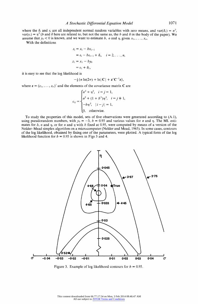
To study the properties of this model, sets of five observations were generated according to (A.1), using pseudorandom numbers, with yo = -3, b = 0.95 and various values for a and 'q. The ML estimates for b, a and a, or for a and i with b fixed at 0.95, were computed by means of a version of the Nelder-Mead simplex algorithm on a microcomputer (Nelder and Mead, 1965). In some cases, contours of the log likelihood, obtained by fixing one of the parameters, were plotted. A typical form of the log likelihood function for b = 0.95 is shown in Figs 3 and 4.

0-045

k. 3*97 Ao2-75

468 004 True

45 0,035 4- 4*45

C. -0 04 -0 03 -0-02 -0 01 0 01 0 02 003 0 04 0

Figure 3. Example of log likelihood contours for b = 0.95.




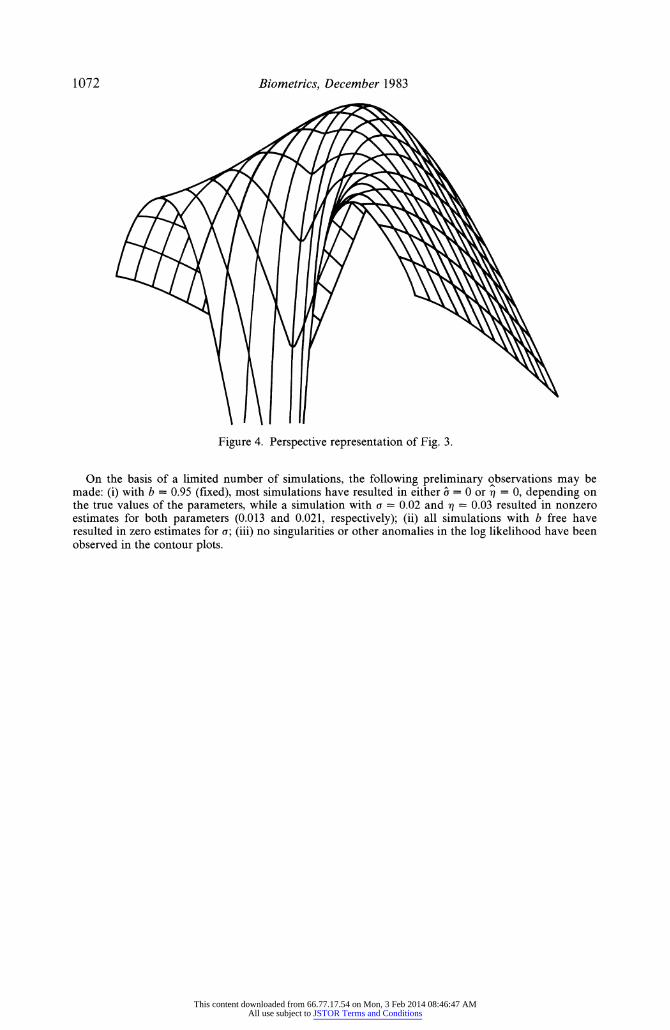
On the basis of a limited number of simulations, the following preliminary observations may be made: (i) with b = 0.95 (fixed), most simulations have resulted in either 'a = 0 or q = 0, depending on the true values of the parameters, while a simulation with a = 0.02 and q = 0.03 resulted in nonzero estimates for both parameters (0.013 and 0.021, respectively); (ii) all simulations with b free have resulted in zero estimates for a; (iii) no singularities or other anomalies in the log likelihood have been observed in the contour plots.

Figure 4. Perspective representation of Fig. 3.



Date post:	22-Dec-2016
Category:	Documents
Upload:	oscar-garcia
View:	212 times
Download:	0 times

A Stochastic Differential Equation Model for the Height Growth of Forest Stands

Documents