A Stochastic Version of Colonel Blotto Game Yosef Rinott * Department of Statistics and Center for the Study of Rationality Hebrew University of Jerusalem Mount Scopus Jerusalem 91905, Israel and LUISS, Roma [email protected]Marco Scarsini Dipartimento di Scienze Economiche e Aziendali LUISS Viale Romania 12 I–00197 Roma, Italy and HEC, Paris [email protected]Yaming Yu Department of Statistics University of California, Irvine CA 92697-1250, USA [email protected]July 26, 2011 * Partially supported by the Israel Science Foundation grant No. 473/04
Transcript
A Stochastic Version of Colonel Blotto Game
Yosef Rinott∗
Department of Statisticsand Center for the Study of Rationality
∗Partially supported by the Israel Science Foundation grant No. 473/04
Abstract
We consider a stochastic version of the well-known Blotto game, called thegladiator game. In this zero-sum allocation game two teams of gladiators en-gage in a sequence of one-to-one fights in which the probability of winning isa function of the gladiators’ strengths. Each team’s strategy consist the allo-cation of its total strength among its gladiators. We find the Nash equilibriaand the value of this class of games and show how they depend on the totalstrength of teams and the number of gladiators in each team. To do this, westudy interesting majorization-type probability inequalities concerning linearcombinations of Gamma random variables. Similar inequalities have been usedin models of telecommunications and research and development.
Keywords and phrases: Allocation game, gladiator game, David and Goliath,sum of exponential random variables, Nash equilibrium, probability inequali-ties, unimodal distribution.
Borel (1921) proposed a game, later dubbed Colonel Blotto game by Gross andWagner (1950). In this game Colonel Blotto and his enemy each have a given (possiblyunequal) amount of resources, that have to be allocated to n battlefields. The sidethat allocates more resources to field j is the winner in this field and gains a positiveamount aj which the other side loses. The war is won by the army that obtains thelargest total gain.
The relevance of Borel precursory insight in the theory of games was discussed inan issue of Econometrica that contains three papers by Borel, including the translationof the 1921 paper (Borel, 1953), two notes by Frechet (1953b,a) and one by vonNeumann (1953).
Borel and Ville (1938) proposed a solution to the game when the two enemieshave an equal amount of resources and there are n = 3 battlefields. The problem wasthen taken up by several authors, including several other famous mathematicians.Gross and Wagner (1950); Gross (1950) provided the solution for a generic n, keepingthe amount of resources equal and the gain in each battlefield constant (ai = aj).Blackett (1954, 1958) considered the case where the payoff to Colonel Blotto in eachbattlefields is an increasing function of his resources and a decreasing function of hisenemy’s resources. Bellman (1969) showed the use of dynamic programming to solvethe Blotto game. Shubik and Weber (1981) studied a more complex model wherethere exist complementaries among the fields being defended. In this case the total
2
payoff depends on the relative value of capturing various configurations of targets.Roberson (2006) used n-copulas to determine the mixed equilibrium of the game undergeneral conditions on the amount of resources for each player. His analysis is based onan interesting analogy with the theory of all-pay auctions (see also Weinstein (2005)for the equilibrium of the game and Sahuguet and Persico (2006) for the connectionbetween all-pay auctions and allocation of electoral promises).
Hart (2008) considered a discrete version of the Blotto game, where player A hasA alabaster marbles and player B has B black marbles. The players are to distributetheir marbles into K urns. One urn is chosen at random and the player with thelargest number of marbles in the chosen urn wins the game. In another version of thegame, called Colonel Lotto game, each player has K urns where she can distributeher marbles. Two urns (one for each player) are chosen at random and the urn withthe larger number of marbles determines the winner. The discrete Colonel Blottogame and the Colonel Lotto game have the same value. In a third version, calledGeneral Lotto game, given a, b > 0, player A chooses a nonnegative integer-valuedrandom variable X with expectation E[X] = a and player B chooses a nonnegativeinteger-valued random variable Y with expectation E[Y ] = b. The payoff for A isP(X > Y )− P(X < Y ), where X and Y are assumed independent. The value of thegame and the optimal strategies are determined.
Other authors who dealt with the Blotto game and its applications include, forinstance, Tukey (1949); Sion and Wolfe (1957); Friedman (1958); Cooper and Restrepo(1967); Penn (1971); Heuer (2001); Kvasov (2007); Adamo and Matros (2009); Powell(2009); Golman and Page (2009) and many more. We refer to Kovenock and Roberson(2010); Chowdhury, Kovenock, and Sheremeta (2010) for some history of the ColonelBlotto game and a good list of references.
In this paper we deal with a stochastic version of the Colonel Blotto game, calledgladiator game by Kaminsky, Luks, and Nelson (1984). In their model two teams ofgladiators engage in a sequence of one-to-one fights. Each gladiator has a strengthparameter. When two gladiators fight, the ratio of their strengths determines theodds of winning. The loser dies and the winner retains his strength and is ready fora new duel. The team that is wiped out loses. Each team chooses the order in whichgladiators go to the arena.
We construct a zero-sum two-team game where each team also has to allocatea fixed total strength among its players. The payoff is linear in the probability ofwinning. We find the Nash equilibria and compute the value of the game. The mainresults are:
(i) the order according to which gladiators fight has no relevance, moreover knowingthe order chosen by the opponent team does not provide any advantage;
(ii) the stronger team always splits its strength uniformly among its gladiators,whereas the weaker team splits the strength uniformly among a subset of itsgladiators;
3
(iii) when the two teams have roughly equal total strengths, the optimal strategy forthe weaker team is to divide its total strength equally among all its members;
(iv) when the total strength of one team is much larger than that of the other, theweaker team should concentrate all the strength on a single member.
De Schuymer, De Meyer, and De Baets (2006) consider a dice game that has someanalogies with ours. Both players can choose one of many dice having n faces andsuch that the total number of pips on the faces of the die is σ. The two dice aretossed and the player with the highest score wins a dollar.
The model described below for the probability that gladiator i defeats j, is equiv-alent, with different parametrization, to the well-known Rasch model in educationalstatistics, (Rasch, 1980), in which the probability of correct response of subject i toitem j is eαi−βj /(1 + eαi−βj) (see Lauritzen, 2008, for a recent mathematical study ofRasch models). A similar model has been used also in the theory of contests proposedby Tullock (1980) (see Corchon, 2007, for a recent survey).
Finding the Nash equilibria of the gladiator game involves an analysis of theprobability of winning. The key step is a result in Kaminsky et al. (1984) thattranslates the calculation of this probability into an inequality involving the sum ofindependent but not necessarily identically distributed exponential random variables.
The main theorems are demonstrated through interesting and hard probabilityinequalities, whose proofs are of independent interest and turned out to be morecomplicated than expected. Much of the paper consists of these proofs. We relyon Szekely and Bakirov (2003) for some of the technical machinery. The problem iscast as a minimization problem involving convolutions of exponential variables and issolved by perturbation arguments. A key identity, derived using Laplace transforms,directs our perturbation arguments to the analysis of the modal location of Gammaconvolutions.
Our inequalities are related to majorization type inequalities for probabilities ofthe form P(Q < t), where Q is a linear combinations of Exponential or Gammavariables, that appear in Bock, Diaconis, Huffer, and Perlman (1987); Diaconis andPerlman (1990); Szekely and Bakirov (2003) and in Telatar (1999); Jorswieck andBoche (2003); Abbe, Huang, and Telatar (2011). The motivation in the last three pa-pers, and numerous others, is the performance of some wireless systems that dependson the coefficients of the linear combination Q. For stochastic comparisons betweensuch linear combinations see Yu (2008, 2011) and references therein.
Linear combinations of exponential variables appear in various other applications.For instance Lippman and McCardle (1987) consider a two-firm model in which learn-ing is stochastic and the research race is divided into a finite number N of stages, eachhaving an exponential completion date. The invention is discovered at the completionof the N -th stage. If the exponential times for one firm have parameters that can becontrolled by the firms subject to constraints, then our results apply to the problemof best response and equilibrium allocation strategies for such races.
4
Finally, it is well known that the first passage time from 0 to N of a birth and deathprocess on the positive integers is distributed as a linear combination of exponentialrandom variables, with coefficients determined by the eigenvalues of the process’generator. For a clear statement, a probabilistic proof, and further references seeDiaconis and Miclo (2009). This allows one to consider R&D type races in which onecan also move backwards, and applies, for example, to the study of queues, where onecompares the time until different systems reach a given queue size.
The paper is organized as follows. In Section 2 we describe the model. In Section 3we determine the Nash equilibria and the value of the game for different values of theparameters. Section 4 contains the main probability inequalities used to compute theequilibria, together with related probability inequalities, that follow from our mainresult and have some interest per se. Section 5 is devoted to proofs.
2 The model
We formalize the model described in the Introduction. Two teams of gladia-tors fight each other according to the following rules. Team A is an ordered setA1, . . . , Am of m gladiators and team B is an ordered set B1, . . . , Bn of n glad-iators. The numbers m,n and the orders of the gladiators in the two teams areexogenously given. At any given time, only two gladiators fight, one for each team.At the end of each fight only one gladiator survives. In each team gladiators go tofight according to the exogenously given order. First gladiators A1 and B1 fight. Thewinner remains in the arena and fights the following gladiator of the opposing team.Assume that for i < m and j < n at some point, Ai fights Bj. If Ai wins, the follow-ing fight will be between Ai and Bj+1; if Ai loses, the following fight will be betweenAi+1 and Bj. The process goes on until a team is wiped out. The other team is thenproclaimed the winner. So if at some point, for some i ≤ m, gladiator Ai fights Bn
and wins, then team A is the winner. Symmetrically if, for some j ≤ n, Am fights Bj
and loses, then team B is the winner.Team A has total strength cA and team B has total strength cB. The values cA
and cB are exogenously given. Before fights start the coach of each team decideshow to allocate the total strength to the gladiators of the team. These decisionsare simultaneous and cannot be altered during the play. Let a = (a1, . . . , am) andb = (b1, . . . , bn) be the strength vectors of team A and B, respectively. This meansthat in team A gladiator Ai gets strength ai and in team B gladiator Bj gets strengthbj. The vectors a, b are nonnegative and such that
m∑i=1
ai = cA,
n∑j=1
bj = cB,
namely, each coach distributes all the available strength among the gladiators of histeam.
5
When a gladiator with strength ai fights a gladiator with strength bj, the firstdefeats the second with probability ai/(ai + bj), all fights being independent. Whena gladiator wins a fight his strength remains unaltered. The rules of the play and itsparameters, i.e., the teams A and B and the strengths cA, cB, are common knowledge.Call Gm,n(a, b) the probability that team A with strength vector a wins over teamB with strength vector b.
The above model gives rise to the zero-sum two-person game
G (m,n, cA, cB) = 〈A (m, cA),B(n, cB), Hm,n〉 (2.1)
in which team A chooses a ∈ A (m, cA) and B chooses b ∈ B(n, cB), where
A (m, cA) =
(a1, . . . , am) ∈ Rm
+ :m∑i=1
ai = cA
, (2.2)
B(n, cB) =
(b1, . . . , bn) ∈ Rn
+ :n∑i=1
bi = cB
, (2.3)
Hm,n = Gm,n −1
2. (2.4)
The payoff of team A is then its probability of victory Gm,n(a, b) minus 1/2. Wesubtracted 1/2 to make the game zero-sum.
As will be shown in Remark 4.2 below, other models with different rules of en-gagement for the gladiators give rise to the same zero-sum game.
3 Main results
Consider the game G defined in (2.1). The action a∗ is a best response against bif
a∗ ∈ arg maxa∈A
Hm,n(a, b).
A pair of actions (a∗, b∗) is a Nash equilibrium of the game G if
Hm,n(a, b∗) ≤ Hm,n(a∗, b∗) ≤ Hm,n(a∗, b), for all a ∈ A (m, cA) and b ∈ B(n, cB).
A pair of actions (a∗, b∗) is a minmax solution of the game G if
maxa∈A (m,cA)
minb∈B(n,cB)
Hm,n(a, b) = minb∈B(n,cB)
maxa∈A (m,cA)
Hm,n(a, b) = Hm,n(a∗, b∗).
Since we are dealing with a finite zero-sum game, Nash equilibria and minmaxsolutions coincide (see, e.g., Osborne and Rubinstein, 1994, Proposition 22.2). Thequantity Hm,n(a∗, b∗) is called the value of the game G .
The next theorem characterizes the structure of Nash equilibria of the gameG (m,n, cA, cB).
6
Theorem 3.1. Consider the game G (m,n, cA, cB) defined in (2.1). Assume thatcA ≤ cB.
(a) Any equilibrium strategy profile (a∗, b∗) of G is of the following form: there existsJ ⊆ 1, . . . ,m such that
a∗i = cA/|J | for i ∈ J, a∗i = 0 for i ∈ J c, (3.1)
b∗i = cB/n for i ∈ 1, . . . , n. (3.2)
(b) If
cB ≤n
n− 1cA, (3.3)
then J = 1, . . . ,m, so that a∗1 = · · · = a∗m = cA/m and b∗1 = · · · = b∗n = cB/n.
(c) If
cB ≥3n
2(n− 1)cA, (3.4)
then J = i, that is a∗i = cA for some i ∈ 1, . . . ,m and a∗j = 0 for all j 6= i,and b∗1 = · · · = b∗n = cB/n.
Theorem 3.1 shows that if a vector a∗ is an equilibrium strategy, then so is anypermutation of a∗. Moreover the team with the highest total strength always dividesit equally among its members, whereas the other team divides its strength equallyamong a subset of its members. This subset coincides with the whole team if thetotal strengths of the two teams are similar, and it reduces to one single gladiator ifthe team has a much lower strength than the other team (see Figures 1, 2, and 3).
FIGURES 1, 2, AND 3 ABOUT HERE
Thus, the strategies proposed by the Philistine Goliath to the Israelites to send outa champion of their own to decide the outcome in a single combat with him (Samuel1, chapter 17) was not optimal for the Philistines, as being the stronger side theyshould have divided their strength equally rather than concentrate it in one Goliath;it was optimal for the much weaker Israelites. For n = 1, i.e., when team B has asingle player, equal strength is always team A’s best strategy.
In order to compute the value of the game G (m,n, cA, cB), we need the regularizedincomplete beta function
I(x, α, β) =1
B(α, β)
∫ x
0
tα−1(1− t)β−1 dt, (3.5)
where
B(α, β) =
∫ 1
0
tα−1(1− t)β−1 dt =Γ(α)Γ(β)
Γ(α + β).
7
When α and β are integers, then
I(x, α, β) =
α+β−1∑j=α
(α + β − 1
j
)xj(1− x)α+β−1−j. (3.6)
For properties of incomplete beta functions see, for instance, Olver, Lozier, Boisvert,and Clark (2010).
Theorem 3.2. Consider the game G (m,n, cA, cB). Assume that cA ≤ cB.
(a) The value of the game is
1
2− I
(rcB
rcB + ncA, r, n
), (3.7)
where r is the number of positive a∗i in the vector a∗. In particular
(b) if (3.3) holds, then the value of the game is
1
2− I
(mcB
mcB + ncA,m, n
), (3.8)
(c) if (3.4) holds, then the value of the game is
1
2− I
(cB
cB + ncA, 1, n
). (3.9)
In general, to compute the value of the game, one only needs to maximize (3.7)over r = 1, . . . ,m; any maximizing r gives an optimal strategy for team A. Figure 4shows the value of the game as cB varies. Different values of cB imply differentnumbers of positive a∗i .
FIGURE 4 ABOUT HERE
FIGURE 5 ABOUT HERE
We mention the following consequence of Theorem 3.1 (see Figure 5).
Corollary 3.3. In the game G (m,n, cA, cB), if the two teams have equal strength(i.e., cA = cB), then the value is positive if m > n, namely, the team with moreplayers has an advantage over the other team. Moreover, the value of the game isincreasing in m and decreasing in n.
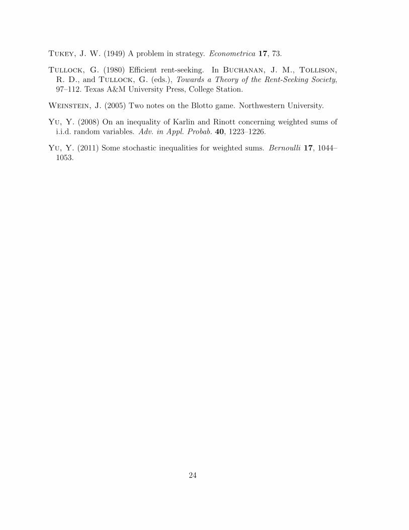
FIGURE 6 ABOUT HERE
8
Figure 6 shows an interesting implication of Theorem 3.2: team B may be at adisadvantage even if cA < cB, and this happens if the number n of its gladiators ismuch smaller than the number m of gladiators in A. As the relative difference instrength between the two teams increases, it takes a larger number of gladiators tocompensate for the lower strength.
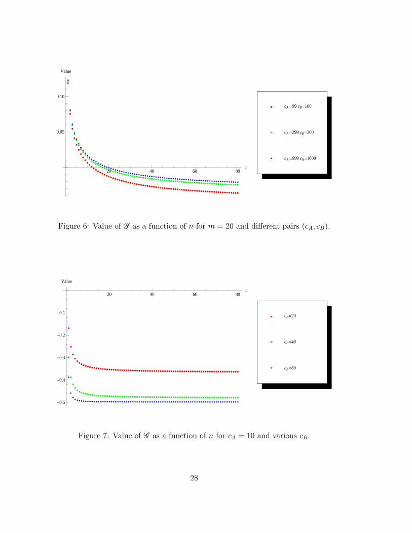
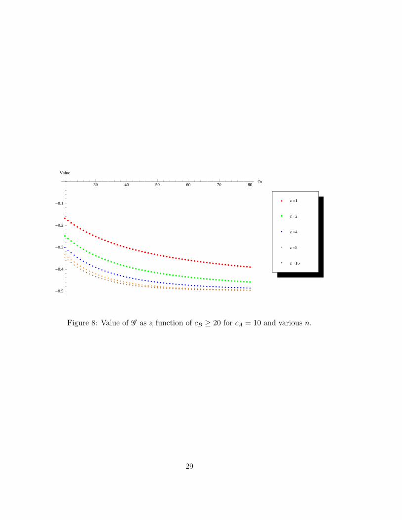
FIGURES 7 AND 8 ABOUT HERE
As Figures 7 and 8 show, if condition (3.4) holds, then team A is at a strongdisadvantage. The disadvantage increases with the total strength cB and the numbern of gladiators of team B. The number m of gladiators of team A is totally irrelevant,since, in equilibrium, the whole strength cA is assigned to only one gladiator.
4 Probability inequalities
We say that X ∼ Exp(1) if X has a standard exponential distribution, i.e., P(X >x) = e−x for x > 0.
The main theorems of this paper rely on the following result.
Proposition 4.1. [Kaminsky et al. (1984)] The probability Gm,n(a, b) of team Adefeating B is
Gm,n(a, b) = P
(m∑i=1
aiXi >n∑j=1
bjYj
), (4.1)
where X1, . . . , Xm, Y1, . . . , Yn are i.i.d. random variables, with X1 ∼ Exp(1).
Remark 4.2. The implication of Proposition 4.1 is that two vectors a,a′ of strengthsthat are equal up to a permutation produce the same probability of victory, that is,the same payoff function (2.4). The same holds for two vectors b, b′. Therefore variousmodels, with different rules for the order in which gladiators fight, give rise to thesame game (2.1). This happens, for instance, in a model where the winning gladiatordoes not stay in the arena to fight the following opponent, but, rather, goes to thebench at the end of his team’s queue, and comes back to fight when his turn comes.This happens also when, at the end of each fight, each coach chooses one of the livinggladiators in his team at random and sends him to fight. Basically, provided theallocations of strength in the two teams is decided simultaneously at the beginningand is not modified throughout, any rule governing the order of descent of gladiatorsin the arena leads to the same game (2.1). This is true also for nonanticipative rulesthat depend on the history of the battles so far. The key assumption for this is thefact that a winning gladiator does not lose (or gain) any strength after a victoriousbattle. This is parallel to the lack-of-memory property in many reliability models, andexplains why the probability of winning (4.1) involves sums of exponential randomvariables.
9
Note that the main result (Theorem 3.1) does not go through if the allocationscan also be decided dynamically as battles unfold. In this case the resulting gameis more complicated and optimal allocations may change according to the observedhistory. For instance consider the case where cB is slightly larger than cA. At thebeginning, suppose team B spreads the strength uniformly across all its players. Ifteam B keeps losing some battles, then it may become optimal to spread the strengthamong only a subset of the surviving players.
The following theorem is the main tool to prove Theorem 3.1.
Theorem 4.3. Let X1, . . . , Xm and Y1, . . . , Yn, m,n ≥ 1, be i.i.d. random variableswith X1 ∼ Exp(1). For fixed b > 0, let A be as in (2.2) and let
(a∗1, . . . , a∗m) ∈ arg min
a∈A (m,m)P
(m∑i=1
aiXi ≤ b
n∑j=1
Yj
).
Then
(a) all nonzero values among a∗1, . . . , a∗m are equal;
(b) if m ≥ (n− 1)b, then a∗1 = · · · = a∗m = 1;
(c) if m ≤ 2(n− 1)b/3, then a∗i = m for a single i, 1 ≤ i ≤ m, and a∗j = 0, for j 6= i.
4.1 Related probability inequalities
If X1, . . . , Xm, and Y1, . . . , Yn are i.i.d. random variables with X1 ∼ Exp(1), and
X =1
m
m∑i=1
Xi, Y =1
n
n∑j=1
Yj, Z =mX
mX + nY,
then Z has a Beta(m,n) distribution. Hence
P(X < Y ) = P(Z <
m
m+ n
)= I
(m
m+ n,m, n
). (4.2)
For m > n, by Corollary 3.3, we have
P(X < Y ) <1
2. (4.3)
Since E[Z] = m/(m + n), (4.3) is equivalent to P (Z < E[Z]) < 1/2, that is, E[Z] <Med[Z]. This is a well known mean-median inequality for beta distributions (seeGroeneveld and Meeden, 1977).
The inequality (4.3) has the following interesting statistical implication. If twostatisticians estimate the mean of exponential variables, and use the sample mean as
10
their unbiased estimate, then the statistician with the larger sample tends to havea larger (unbiased) estimate. If the two of them bet on who has a larger estimate,the one with the larger sample tends to win. For normal variables, or any symmetricvariables, this clearly cannot happen and P(X < Y ) = 1/2.
Suppose now that the two statisticians share the first n variables, that is, for i =1, . . . , n we have Xi = Yi, and the remaining variables Xn+1, . . . , Xm are independentof the previous ones. Then
P(X < Y ) = P
(1
m
[n∑j=1
Yj +m∑
i=n+1
Xi
]<
1
n
n∑j=1
Yj
)
= P
(1
m− n
m∑i=n+1
Xi <1
n
n∑j=1
Yj
). (4.4)
By (4.3) the last expression in (4.4) is less than 1/2 if and only if m− n > n, that is,m > 2n. It equals 1/2 if m = 2n, and it is larger than 1/2 if m < 2n, in which case(4.3) is reversed. Thus in the bet between the statisticians, if most of the variablesare in common, the odds are against the one with the larger sample, contrary to theprevious situation. This was noted by Abram Kagan.
Our main results can be presented in terms of various other distributional inequal-ities or monotonicity. Using (3.6) and Corollary 3.3 we obtain further results thatcannot easily be proved more directly. We say that X ∼ Gamma(α, β) if X has adensity
f(x) =βα
Γ(α)e−βx xα−1, x > 0.
Corollary 4.4. The following properties hold:
(a) The function
I
(m
m+ n,m, n
)is decreasing in m for fixed n, and increasing in n for fixed m.
(b) Let T ∼ Binom(m+ n− 1,m/(m+ n)). Then P(T ≥ m) is decreasing in m andincreasing in n.
(c) Let S ∼ Poisson(m). Then P(S ≥ m) is decreasing in m.
(d) Let R ∼ Gamma(m, 1). Then P(R ≤ m) is decreasing in m.
We say that a random variable Q ∼ Geom(p) if P(Q1 = k) = (1 − p)kp, k =0, 1, 2, . . . .
Proposition 4.5. Let Q1, . . . , Qm be independent random variables such that Qi ∼Geom(1/(1 + ai)). Define Q =
∑mi=1Qi.
11
(a) We have1−Gm,n(a,1n) = P (Q ≤ n− 1) , (4.5)
where a = (a1, . . . , am) and 1n denotes the n-dimensional vector of ones.
(b) If∑m
i=1 ai = n, then the probability in (4.5) is minimized when all ai’s are equal.In this case Qi are i.i.d. and Q has a negative binomial distribution.
(c) If E[Q] = m, then E[Q] > Med[Q].
5 Proofs
The long path to the proof of Theorem 3.1 goes through the following steps: firstwe provide a short proof of Proposition 4.1 for the sake of completeness. Then westate and prove three lemmas needed for the proof of Theorem 4.3. Then we proveTheorem 4.3, and, resorting to it, we finally prove Theorem 3.1.
Proof of Proposition 4.1. First note that if X, Y are i.i.d. random variables withX ∼ Exp(1), then P(aX > bY ) = a/(a + b). Therefore, one can see a duel be-tween gladiators i and j as a competition in which the probability of winning is theprobability of living longer, when their lifetimes are aiX and bjY , respectively. It isthen easy to understand that the teams’ total lives are
∑mi=1 aiXi and
∑nj=1 bjYj, and
the probability that team A wins is that it lives longer, which is Gm,n(a, b), so (4.1)follows.
In order to prove Theorem 4.3 we need several preliminary results. LetG1, G2, Z1, Z2
be independent with Gi ∼ Gamma(ui, 1), Zi ∼ Exp(1), for i = 1, 2. For ui = 0 wedefine Gi = 0 with probability 1.
Lemma 5.1. Given a∗1, a∗2, set a1 = a∗1 + δ/u1 and a2 = a∗2 − δ/u2. Then
∂
∂δP(a1G1 + a2G2 ≤ x) = (a1 − a2)
∂2
∂x2P(a1(G1 + Z1) + a2(G2 + Z2) ≤ x). (5.1)
Proof. Let
F (x) = P(a1G1 + a2G2 ≤ x)
H(x) = P(a1G1 + a2G2 + a1Z1 + a2Z2 ≤ x)
and let f and h denote the corresponding densities. Let L denote the Laplacetransform, that is,
For the left hand side of (5.2) note that we can interchange differentiation and inte-gration, and also that
∂
∂δL (F (x)) = L (F (x))
∂
∂δlog L (F (x)).
Again by integration by parts we have
L (F (x)) =1
tL (f(x)) =
1
tE[exp−t(a1G1 + a2G2)].
It follows that (5.2) is equivalent to
1
t
∂
∂δlog L (f(x)) = (a1 − a2) t E[exp−t(a1Z1 + a2Z2)]. (5.3)
Explicitly this becomes
1
t
∂
∂δlog[(1 + a1t)
−u1(1 + a2t)−u2 ] = (a1 − a2)t(1 + a1t)
−1(1 + a2t)−1. (5.4)
Using a1 = a∗1 + δ/u1, and a2 = a∗2 − δ/u2, (5.4) is verified by a straightforwardcalculation.
A related result to Lemma 5.1, with a similar type of proof, appears in Szekelyand Bakirov (2003).
Lemma 5.2. Given a nonnegative vector (a∗1, . . . , a∗m), let
a1 = a∗1 + δ/u1, a2 = a∗2 − δ/u2, ai = a∗i for 3 ≤ i ≤ m.
Define
Q(a,u) =m∑i=1
aiGi − bn∑j=1
Yj, (5.5)
where (a,u) := (a1, . . . , am, u1, . . . , um), G1, . . . , Gm, Y1, . . . , Yn are independent ran-dom variables with Gi ∼ Gamma(ui, 1), for i = 1, . . . ,m and Yj ∼ Exp(1), forj = 1, . . . , n. Let Zi ∼ Exp(1), for i = 1, 2 be independent of all other variables.Then
∂
∂δP(Q(a,u) ≤ x) = (a1 − a2)
∂2
∂x2P(Q(a,u) + a1Z1 + a2Z2 ≤ x). (5.6)
13
Proof. Set T =∑m
i=3 aiGi − b∑n
j=1 Yj. Then
∂
∂δP(Q(a,u) ≤ x|T ) = (a1 − a2)
∂2
∂x2P(Q(a,u) + a1Z1 + a2Z2 ≤ x|T ), (5.7)
which is equivalent to (5.1) with a different x. Taking the expectation in (5.7) overT yields (5.6).
Lemma 5.3. Let X and Y be independent random variables where Y ∼ Exp(1) andX has a density f(x) such that
(i) f(x) is continuously differentiable with a bounded derivative on (−∞,∞),
(ii) f(x) > 0 for sufficiently small x ∈ (−∞,∞),
(iii) f(x) is unimodal, i.e., there exists a ∈ (−∞,∞) such that f ′(x) ≥ 0 if x < aand f ′(x) ≤ 0 if x > a.
For λ > 0, denote the density of X + λY by fλ(x). Then fλ(x) is unimodal and iff ′λ(x0) = 0 then x0 is a mode of fλ. Moreover, if λ > λ0 > 0, then any mode of fλ(x)is strictly larger than any mode of fλ0(x).
Proof. This result is similar to Szekely and Bakirov (2003, Lemma 1). We provide aquick proof using variation diminishing properties of sign regular kernels (see Karlin,1968). First, since the density of λY is log-concave (a.k.a. strongly unimodal) itsconvolution with the unimodal f(x) is also unimodal, that is, the pdf of X + λY isunimodal (see Ibragimov, 1956; Karlin, 1968).
Differentiating yields
f ′λ(x) =
∫ ∞0
f ′(x− z)1
λe−z/λ dz
=
∫ x
−∞f ′(z)
1
λe(z−x)/λ dz
=e−x/λ
λ
∫1(−∞,x)(z)f ′(z) ez/λ dz.
Suppose f ′λ(x0) = 0. Since f ′(z) ≥ 0 for z ≤ a, we know from the representationabove that f ′λ(x) > 0 if x ≤ a, and hence x0 > a. The representation also showsthat the function ex/λ f ′λ(x) is nonincreasing in x ∈ (a,∞). Therefore f ′λ(x) ≥ 0 ifx ∈ (a, x0) and f ′λ(x) ≤ 0 if x > x0. It follows that x0 is a mode of fλ(x).
For fixed x, the function 1(−∞,x)(z)f ′(z) as a function of z has at most one signchange from positive to negative, and the kernel ez/λ is strictly reverse rule (seeKarlin, 1968). It follows that
∫1(−∞,x)(z)f ′(z) ez/λ dz has at most one sign change
from negative to positive, as a function of λ. Thus, if for a given x, f ′λ0(x) = 0 andλ > λ0, then f ′λ(x) > 0, and the result follows.
14
Proof of Theorem 4.3. LetQ(a) := Q(a,1m) as in (5.5). Consider minimizing P(Q(a) ≤0) over
Ω =
a : 0 ≤ ai,
m∑i=1
ai = m
.
Since Ω is compact, and P(Q ≤ 0) is continuous in a, the minimum is attained, say,at a∗ ∈ Ω.
Claim 5.4. In any minimizing point a∗ of P(Q ≤ 0) the a∗i ’s take at most two distinctnonzero values. Moreover, in the case of two distinct nonzero values, the smaller oneappears only once.
Proof. Assume the contrary, say 0 < a∗1 ≤ a∗2 < a∗3. We show below in Case 1 thatmore than two distinct values are impossible by showing that a∗1 < a∗2 leads to acontradiction. Similarly Case 2 implies the impossibility of repetitions of the smallestof two distinct values. Let a1 = a∗1 + δ, a2 = a∗2 − δ, ai = a∗i , 3 ≤ i ≤ m. Then by(5.6) we have
∂
∂δP(Q(a) ≤ x) = (a1 − a2)
∂2
∂x2P(Q(a) + a1Z1 + a2Z2 ≤ x), (5.8)
where Z1 and Z2 are i.i.d. random variables with Z1 ∼ Exp(1), independent of Q.We can focus on x = 0.
Case 1. a∗1 < a∗2. Since δ = 0 achieves the minimum, both sides of (5.8) with x = 0vanish at δ = 0. The density function of Q(a∗) + a∗1Z1 is positive everywhere andis log-concave and hence unimodal. By Lemma 5.3, S = Q(a∗) + a∗1Z1 + a∗2Z2 has amode at zero. Following Case 2 we show that this leads to a contradiction.
Case 2. a∗1 = a∗2. Then (5.8) gives
limδ↓0
∂P(Q(a) ≤ 0)
∂δ= 0
and∂2
∂δ2P(Q(a) ≤ 0)
∣∣∣∣δ=0
= 2 limδ→0
∂2
∂x2P(Q(a) + a1Z1 + a2Z2 ≤ x)
∣∣∣∣x=0
.
A minimum at δ = 0 entails
∂2
∂x2P(Q(a∗) + a∗1Z1 + a∗2Z2 ≤ x)
∣∣∣∣x=0
≥ 0,
showing that S = Q(a∗) + a∗1Z1 + a∗2Z2 has a mode that is nonnegative.
15
Thus S has a nonnegative mode in either case. By Lemma 5.3 and a∗2 < a∗3, anymode of Q(a∗) + a∗1Z1 + a∗3Z2 is strictly positive, i.e.,
∂2
∂x2P(Q(a∗) + a∗1Z1 + a∗3Z2 ≤ x)
∣∣∣∣x=0
> 0.
The latter expression, multiplied by (a∗1−a∗3) is negative. Using (5.8) with a∗3 in placeof a∗2, however, this implies that P(Q(a) ≤ 0) strictly decreases under the perturbation(a∗1, a
∗3)→ (a∗1 + δ, a∗3 − δ) for small δ > 0, which is a contradiction to the minimality
at δ = 0. Note that the crux of the proof is in comparing two perturbations.
Claim 5.5. In any minimizing point a∗ of P(Q ≤ 0) the a∗i ’s are either all equal, ortake only two distinct values, in which case one of them is zero.
Proof. Assume the contrary, and in view of Claim 5.4, suppose we have
with X ∼ Exp(1), G ∼ Gamma(k, 1), Y ∼ Gamma(n, 1) independently. We showthat the minimum of P(Q(a) ≤ 0) cannot be achieved in the open interval δ ∈ (0, 1/k),contradicting the assumption that a∗ is a minimizer. We have
P(Q(a) ≤ 0) = P(
1 + δ(1− (k + 1)B) ≤ λY
X +G
),
where B := X/(X + G). Note that B has a Beta(1, k) distribution, Y/(X + G) hasa scaled F (2n, 2(k + 1)) distribution, and B and Y/(X +G) are independent. Thus
P(Q(a) ≤ 0) = C1 E[∫ ∞
1+δ(1−(k+1)B)
yn−1
(λ+ y)n+k+1dy
].
where above and below, Ci > 0 denote constants that do not depend on δ, andDi(δ) > 0 denote functions of δ ∈ (0, 1/k), and both may depend on other constantssuch as λ, k, etc. It follows that
It is helpful to determine the sign of g(δ) for small δ > 0 and large δ < 1/k. Let usdenote the integral in (5.9) by g(δ), which has the same sign as g(δ) for δ ∈ (0, 1/k).A Taylor expansion yields
g(δ) =
∫ 1
−k
[x(x+ k)k−1
(λ+ 1)n+k+1+
(λ(n− 1)− k − 2)δ
(λ+ 1)n+k+2x2(x+ k)k−1
]dx+ o(δ)
= C3(λ(n− 1)− k − 2)δ + o(δ), as δ ↓ 0.
By direct calculation,g(1/k) = C4(λ(n− 1)− k − 1).
We distinguish three cases:
(i) λ(n− 1) > k+ 2. Then g(δ) > 0 and hence g(δ) > 0 for sufficiently small δ > 0.Moreover, by (5.11), g′(δ) > D3(δ)g(δ), δ ∈ (0, 1/k). It follows that g(δ) > 0for all δ ∈ (0, 1/k), i.e., P(Q(a) ≤ 0) decreases in δ ∈ [0, 1/k]. The same holdsin the boundary case λ(n− 1) = k + 2.
17
(ii) k+1 < λ(n−1) < k+2. Then g(δ) < 0 for sufficiently small δ > 0, and g(δ) > 0for sufficiently large δ < 1/k. If the minimum of P(Q(a) ≤ 0) is achieved atδ∗ ∈ (0, 1/k), then g(δ∗) = 0 ≥ g′(δ∗), and g(δ) has at least one root in (0, δ∗),say δ∗∗, such that g′(δ∗∗) ≥ 0. This contradicts (5.11), however, because theterm in square brackets strictly increases in δ.
(iii) λ(n−1) < k+1. Then g(δ) < 0 for both sufficiently large δ < 1/k and sufficientlysmall δ > 0. Suppose g(δ∗) > 0 for some δ∗ ∈ (0, 1/k). If λn > k then acontradiction results as in Case (ii). Otherwise the term in square brackets in(5.11) is no more than
(λ+ 1)(k − 1)k−1 + (λ+ 1)(λ(n− 1)− k − 2) < 0.
Thus any δ ∈ (0, 1/k) such that g(δ) = 0 entails g′(δ) < 0. This is impossibleas g(δ) cannot cross zero from above without first doing so from below. Henceg(δ) ≤ 0, i.e., P(Q(a) ≤ 0) increases in δ ∈ [0, 1/k]. The same holds in theboundary case λ(n− 1) = k + 1.
We now prove the three statements of Theorem 4.3.
(a) This is an immediate consequence of Claim 5.5.
(b) Let h(k) = P(Q(a) ≤ 0) with
a1 = · · · = ak =m
k, 1 ≤ k ≤ m, and ak+1 = · · · = am = 0.
Comparing P(Q(a) ≤ 0) in Case (iii) of the proof of Claim (5.5) at δ = 0 andδ = 1/k, we see that if m ≥ b(n− 1), i.e.,
b(k + 1)(n− 1)
m≤ k + 1,
then h(k + 1) < h(k), 1 ≤ k < m. Thus h(k) achieves its minimum at k = m.
(c) Suppose now m < b(n−1). According to Case (i), if b(k+ 1)(n−1)/m ≥ k+ 2,i.e.,
k + 1 ≥ m
(b(n− 1)−m), (5.12)
then h(k + 1) > h(k). In particular, (5.12) holds for all k if m ≤ 2b(n − 1)/3,which yields h(m) > · · · > h(2) > h(1), i.e., h(k) is minimized at k = 1. Ingeneral h(k) is minimized at some k ≤ dm/(b(n− 1)−m)− 1e.
18
Proof of Theorem 3.1. (a) Using Proposition 4.1 and Theorem 4.3(a), once all theai are multiplied by a factor cA/m, we can prove that a strategy profile thatsatisfies (3.1) and (3.2) is a Nash equilibrium. Assume ad absurdum the exis-
tence of an equilibrium (a, b) that does not satisfy (3.1) and (3.2). Because thegame is zero-sum, we have
Hm.,n(a, b) ≥ Hm,n(a∗, b) > Hm,n(a∗, b∗)
andHm,n(a, b) ≤ Hm,n(a, b∗) < Hm,n(a∗, b∗),
which is a contradiction. Therefore any equilibrium satisfies (3.1) and (3.2).
(b) Theorem 4.3(b) guarantees that if a∗1 = · · · = a∗m = cA/m and b∗1 = · · · = b∗n =cB/n, then a∗ is the unique best response to b∗ and vice versa. This provesthat (a∗, b∗) is a Nash equilibrium of the game. Applying the same reductio adabsurdum used in part (a) we prove that the equilibrium (a∗, b∗) is unique.
(c) Theorem 4.3(c) guarantees that if a∗i = cA for some i ∈ 1, . . . ,m and a∗j = 0for all j 6= i, and b∗1 = · · · = b∗n = cB/n, then a∗ is a best response to b∗
and Theorem 4.3(b) guarantees that b∗ is the unique best response to a∗. Thisproves that (a∗, b∗) is a Nash equilibrium of the game. Again the argumentused in part (a) shows that all Nash equilibria are of this form.
Proof of Theorem 3.2. (a) Using Theorem 3.1(a) we know that for some 1 ≤ r ≤ mand some permutation π we have a∗π(1) = · · · = a∗π(r) = cA/r, aπ(r+1) = · · · =
aπ(m) = 0, and b∗1 = · · · = b∗n = cB/n. Hence
m∑i=1
a∗iXi ∼ Gamma(r, r/cA),n∑j=1
b∗jYj ∼ Gamma(n, n/cB).
Therefore, (see, e.g, Cook and Nadarajah, 2006; Cook, 2008)
P
(m∑i=1
a∗iXi >
n∑j=1
b∗jYj
)= 1− I
(rcB
rcB + ncA, r, n
),
where I is the regularized incomplete beta function defined in (3.5).
(b) By Theorem 3.1(b) in this case r = m.
(c) By Theorem 3.1(c) in this case r = 1.
19
Proof of Corollary 3.3. The team with more players always has the option of notusing them all. Therefore it cannot be worse off than the team with fewer players.However, since equal allocation is the unique best response, using them all is strictlybetter. The same argument proves the monotonicity in m and n. Note that directlyverifying this from the properties of the incomplete beta function appears nontrivial.
Proof of Corollary 4.4. (a) is a restatement of the last part of Corollary 3.3.
(b) follows from (a) and (3.6).
(c) follows from (b) by letting n→∞.
(d) follows from (c) and the identity
P(S ≥ m) =1
Γ(m)
∫ m
0
e−t tm−1 dt.
Proof of Proposition 4.5. (a) The relation (4.5) can be explained directly: team Aloses if all its gladiators together defeat at most n − 1 opponents. Gladiator ifrom team A defeats a geometric random number, Qi, of gladiators of strength1 from team B since he fights until he loses, and he loses a fight with probability1/(1+ai). Thus if
∑mi=1Qi ≤ n−1, then team A defeats at most n−1 gladiators
altogether, and loses.
(b) This follows directly from Theorem 4.3.
(c) Note that E[Q] =∑m
i=1 ai. Letting n = m, and using (4.5) and part (b), weconclude that P(Q ≤ n − 1) ≥ 1 − Gm,n(1m,1n) = 1/2. We obtain P(Q ≤E[Q]) = P(Q ≤ n) > 1/2, and therefore E[Q] > Med[Q].
Acknowledgements
The gladiator game of Kaminsky et al. (1984) was pointed to us by Gil Ben Zvi.We are grateful to Sergiu Hart, Pierpaolo Brutti, Abram Kagan, Paolo Giulietti, andChris Peterson for their interest and excellent advice.
References
Abbe, E., Huang, S.-L., and Telatar, E. (2011) Proof of the outage probabilityconjecture for MISO channels. ArXiv 1103.5478.
20
Adamo, T. and Matros, A. (2009) A Blotto game with incomplete information.Econom. Lett. 105, 100–102.
Bellman, R. (1969) On “Colonel Blotto” and analogous games. SIAM Rev. 11,66–68.
Blackett, D. W. (1954) Some Blotto games. Naval Res. Logist. Quart. 1, 55–60.
Blackett, D. W. (1958) Pure strategy solutions of Blotto games. Naval Res. Logist.Quart. 5, 107–109.
Bock, M. E., Diaconis, P., Huffer, F. W., and Perlman, M. D. (1987)Inequalities for linear combinations of gamma random variables. Canad. J. Statist.15, 387–395.
Borel, E. (1921) La theorie des jeux et les equations integrales a noyau symetrique.C. R. Acad. Sci. Paris 173, 1304–1308.
Borel, E. (1953) The theory of play and integral equations with skew symmetrickernels. Econometrica 21, 97–100.
Borel, E. and Ville, J. (1938) Application de la Theorie des Probabilites auxJeux de Hasard. Gauthier-Villars. Reprinted in Borel, E., and Cheron, A. (1991).Theorie Mathematique du Bridge a la Portee de Tous, Editions Jacques Gabay.
Chowdhury, S. M., Kovenock, D., and Sheremeta, R. M. (2010) An experi-mental investigation of Colonel Blotto games. Working Paper 2688, CESifo.
Cook, J. D. (2008) Numerical computation of stochastic inequality probabilities.Technical Report 46, UT MD Anderson Cancer Center Department of Biostatistics.
Cook, J. D. and Nadarajah, S. (2006) Stochastic inequality probabilities foradaptively randomized clinical trials. Biom. J. 48, 356–365.
Cooper, J. N. and Restrepo, R. A. (1967) Some problems of attack and defense.SIAM Rev. 9, 680–691.
Corchon, L. (2007) The theory of contests: a survey. Review of Economic Design11, 69–100.
De Schuymer, B., De Meyer, H., and De Baets, B. (2006) Optimal strategiesfor equal-sum dice games. Discrete Appl. Math. 154, 2565–2576.
Diaconis, P. and Miclo, L. (2009) On times to quasi-stationarity for birth anddeath processes. J. Theoret. Probab. 22, 558–586.
21
Diaconis, P. and Perlman, M. D. (1990) Bounds for tail probabili-ties of weighted sums of independent gamma random variables. In Top-ics in Statistical Dependence (Somerset, PA, 1987), volume 16 of IMS Lec-ture Notes Monogr. Ser., 147–166. Inst. Math. Statist., Hayward, CA. URLhttp://dx.doi.org/10.1214/lnms/1215457557.
Frechet, M. (1953a) Commentary on the three notes of Emile Borel. Econometrica21, 118–124.
Frechet, M. (1953b) Emile Borel, initiator of the theory of psychological gamesand its application. Econometrica 21, 95–96.
Friedman, L. (1958) Game-theory models in the allocation of advertising expendi-tures. Operations Res. 6, 699–709.
Golman, R. and Page, S. (2009) General Blotto: games of allocative strategicmismatch. Public Choice 138, 279–299. 10.1007/s11127-008-9359-x.
Groeneveld, R. A. and Meeden, G. (1977) The mode, median, and mean in-equality. Amer. Statist. 31, 120–121.
Gross, O. and Wagner, R. (1950) A continuous Colonel Blotto game. TechnicalReport RM-408, RAND Corporation, Santa Monica.
Gross, O. A. (1950) The symmetric Blotto game. Technical Report RM-424, RANDCorporation, Santa Monica.
Hart, S. (2008) Discrete Colonel Blotto and General Lotto games. Internat. J.Game Theory 36, 441–460.
Heuer, G. A. (2001) Three-part partition games on rectangles. Theoret. Comput.Sci. 259, 639–661.
Ibragimov, I. A. (1956) On the composition of unimodal distributions. TheoryProbab. Appl. 1, 255–260.
Jorswieck, E. and Boche, H. (2003) Behavior of outage probability in MISOsystems with no channel state information at the transmitter. In InformationTheory Workshop, 2003. Proceedings. 2003 IEEE, 353–356.
Kaminsky, K. S., Luks, E. M., and Nelson, P. I. (1984) Strategy, nontransitivedominance and the exponential distribution. Austral. J. Statist. 26, 111–118.
Karlin, S. (1968) Total Positivity. Vol. I. Stanford University Press, Stanford, Calif.
Kovenock, D. and Roberson, B. (2010) Conflicts with multiple battlefields.Working paper 3165, CESifo.
22
Kvasov, D. (2007) Contests with limited resources. J. Econom. Theory 136, 738 –748.
Lauritzen, S. L. (2008) Exchangeable Rasch matrices. Rend. Mat. Appl. (7) 28,83–95.
Lippman, S. A. and McCardle, K. F. (1987) Dropout behavior in R&D raceswith learning. RAND J. Econ. 18, 287–295.
von Neumann, J. (1953) Communication on the Borel notes. Econometrica 21,124–127.
Olver, F. W. J., Lozier, D. W., Boisvert, R. F., and Clark, C. W. (eds.)(2010) NIST Handbook of Mathematical Functions. U.S. Department of CommerceNational Institute of Standards and Technology, Washington, DC.
Osborne, M. J. and Rubinstein, A. (1994) A Course in Game Theory. MITPress, Cambridge, MA.
Penn, A. I. (1971) A generalized Lagrange-multiplier method for constrained matrixgames. Operations Res. 19, 933–945.
Powell, R. (2009) Sequential, nonzero-sum “Blotto”: allocating defensive resourcesprior to attack. Games Econom. Behav. 67, 611–615.
Rasch, G. (1980) Probabilistic Models for Some Intelligence and Attainment Tests.Chicago: The University of Chicago Press. Expanded version of the 1960 editionpublished by Danish Institute for Educational Research, Copenhagen.
Roberson, B. (2006) The Colonel Blotto game. Econom. Theory 29, 1–24.
Sahuguet, N. and Persico, N. (2006) Campaign spending regulation in a modelof redistributive politics. Econom. Theory 28, 95–124.
Shubik, M. and Weber, R. J. (1981) Systems defense games: Colonel Blotto,command and control. Naval Res. Logist. Quart. 28, 281–287.
Sion, M. and Wolfe, P. (1957) On a game without a value. In Contributionsto the Theory of Games, vol. 3, Annals of Mathematics Studies, no. 39, 299–306.Princeton University Press, Princeton, N. J.
Szekely, G. J. and Bakirov, N. K. (2003) Extremal probabilities for Gaussianquadratic forms. Probab. Theory Related Fields 126, 184–202.
Telatar, E. (1999) Capacity of multi-antenna Gaussian channels. European Trans-actions on Telecommunications 10, 585–595.
23
Tukey, J. W. (1949) A problem in strategy. Econometrica 17, 73.
Tullock, G. (1980) Efficient rent-seeking. In Buchanan, J. M., Tollison,R. D., and Tullock, G. (eds.), Towards a Theory of the Rent-Seeking Society,97–112. Texas A&M University Press, College Station.
Weinstein, J. (2005) Two notes on the Blotto game. Northwestern University.
Yu, Y. (2008) On an inequality of Karlin and Rinott concerning weighted sums ofi.i.d. random variables. Adv. in Appl. Probab. 40, 1223–1226.
Yu, Y. (2011) Some stochastic inequalities for weighted sums. Bernoulli 17, 1044–1053.


![Colonel Blotto On Facebook: The Effect of Social Relations ...€¦ · The Colonel Blotto game was proposed by Borel [5]. It attracted a lot of research after it was used to model](https://static.documents.pub/doc/80x56/5f04bd957e708231d40f7868/colonel-blotto-on-facebook-the-effect-of-social-relations-the-colonel-blotto.jpg)

