Title A stochastic view on the deterministic Navier-Stokes equation Stochastic differential geometry and mathematical physics - Rennes, June 2021 Ana Bela Cruzeiro . Dep. Mathematics IST and Grupo de Física-Matemática Univ. Lisboa 1 / 24
Transcript
Title
A stochastic view on the deterministicNavier-Stokes equation
Stochastic differential geometry and mathematical physics -Rennes, June 2021
Ana Bela Cruzeiro.
Dep. Mathematics IST andGrupo de Física-Matemática Univ. Lisboa
1 / 24
Title
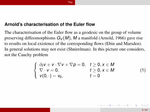
Arnold’s characterisation of the Euler flow
The characterisation of the Euler flow as a geodesic on the group of volumepreserving diffeomorphisms GV (M), M a manifold (Arnold, 1966) gave riseto results on local existence of the corresponding flows (Ebin and Marsden).In general solutions may not exist (Shnirelman). In this picture one considers,not the Cauchy problem
∂tv + v · ∇v +∇p = 0, t ≥ 0, x ∈ M∇ · v = 0, t ≥ 0, x ∈ Mv(0, ·) = v0, t = 0
(1)
2 / 24
Title
but rather ∂tv + v · ∇v +∇p = 0, 0 ≤ t ≤ 1∇ · v = 0, 0 ≤ t ≤ 1gv
1 = h(2)
where gt is the Lagrangian flow gt = v(gt ), g0 = x ∈ M, h a vol.preserving diffeom.
The Lagrangian flow solves the variational problem in GV
min12
∫[0,1]×M
|∂tgt (x)|2dtdx , g0 = Id , g1 = h
and v is recovered by v(t , x) = (∂tgt )(g−1t (x)).
3 / 24
Title
From the Geometric Mechanics point of view, Euler equation is aparticular case of Euler-Poincaré equations, which, in a general (rightinvariant) Lie group read
∂tv(t) = −ad∗v(t)v(t)
when applied to the diffeomorphisms group GV .
4 / 24
Title
Navier-Stokes
The variational principle was extended to the Navier-Stokes equation, usingstochastic flows (ABC, Cipriano, Arnaudon...)Let gv be an incompressible L2 stochastic flow with covariance 2νg−1, whereg is the metric on M , and drift v ; denote Dgv
t (x) = v(t ,gvt (x)).
dgvt (x)⊗ dgv
t (x) = 2νg−1(gvt (t)(x))dt
GeneratorLv = ν∆ + ∂v ,
∆ Laplace-Beltrami.Such flows are known to exist on compact symmetric spaces and on compactLie groups.
5 / 24
Title
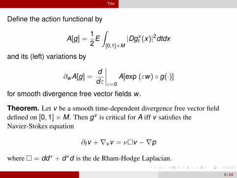
Define the action functional by
A[g] =12
E∫[0,1]×M
|Dgvt (x)|2dtdx
and its (left) variations by
∂wA[g] =ddε
∣∣∣∣ε=0
A[exp (εw) g(·)]
for smooth divergence free vector fields w .
Theorem. Let v be a smooth time-dependent divergence free vector fielddefined on [0,1]×M . Then gv is critical for A iff v satisfies theNavier-Stokes equation
∂tv +∇v v = νv −∇p
where = dd∗ + d∗d is the de Rham-Hodge Laplacian.
6 / 24
Title
In Stochastic Geometric Mechanics, this equation is, as in the classicalcase, an application to GV of the stochastic Euler-Poincaré reductionmethod:
∂tv(t) = −ad∗v(t)v(t) + K (v(t))
where K is some second order positive operator.
Many other dissipative systems can be studied in this way(Camassa-Holm, MHD, etc).
7 / 24
Title
Probabilistic methods for existence of solution:
a possible approach is via forward-backward sde’s, since, after achange of sign, u(t , x) = −v(1− t , x), the solution of
In the rest of the talk we adopt a weaker approach.
8 / 24
Title
Brenier’s generalised framework (for Euler)
One minimises a kinetic energy, but now averaged by probability measures Qon the path space Ω = C([0,1]; M)
min12
EQ
∫ 1
0‖Xt‖2dt , Q01 = π,
Q01 := (X0,X1)∗Q.Here dQt = dx ∀t (Qt = (Xt )∗Q) and π is a probability measure onM ×M s.t. its marginals satisfy dπ0 = dπ1 = dx . The solutions P onlycharge absolutely continuous paths, since the kinetic energy is understood tobe∞ otherwise.
Then
dPt = dx ∀t and P01 = π
Xt +∇p(t ,Xt ) = 0, ∀t , P − a.e.
9 / 24
Title
In this approach one recovers the velocity field by defining a probabilitymeasure σ on [0,1]×M × TM,∫
f (t , x , v)σ(dt ,dx ,dv) :=
∫ 1
0
∫f (t ,Xt , Xt )dP
as DiPerna-Majda solutions;
From now on we consider M = T the torus.
Introducing viscosity
In the spirit of the stochastic approach before, we consider Brownian-typepaths (not abs. continuous). For Q the crresponding law on the path space,kinetic energy is replaced by the forward “mean" velocity:
v
Qt := lim
h→0+
1h
EQ(Xt+h − Xt | X[0,t])
10 / 24
Title
Consider the reference measure R
R =
∫Rxdx ,
Rx the law of the Brownian motion starting from x with diffusionconstant
√2ν.
On the other hand recall the notion of relative entropy of a measure Qwith respect to a measure R
H(Q|R) :=
∫log(
dQdR
) dQ ∈ (−∞,∞]
11 / 24
Title
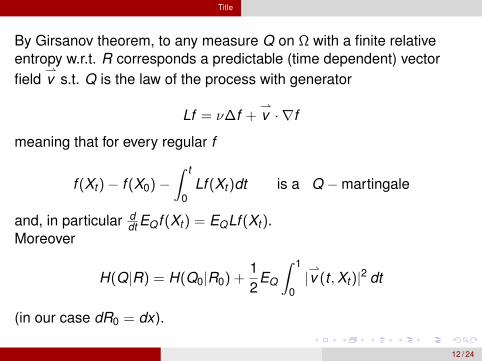
By Girsanov theorem, to any measure Q on Ω with a finite relativeentropy w.r.t. R corresponds a predictable (time dependent) vectorfield
v s.t. Q is the law of the process with generator
Lf = ν∆f +v · ∇f
meaning that for every regular f
f (Xt )− f (X0)−∫ t
0Lf (Xt )dt is a Q −martingale
and, in particular ddt EQf (Xt ) = EQLf (Xt ).
Moreover
H(Q|R) = H(Q0|R0) +12
EQ
∫ 1
0|v (t ,Xt )|2 dt
(in our case dR0 = dx).
12 / 24
Title
So we naturally consider the problem
min12
EQ
∫ 1
0|v (t ,Xt )|2 dt
with Q01 = π and Qt = µt prescribed measures on T (Lebesguemeasure for incompressibility constraint), which is the entropyminimisation problem. We may ask only Qt = µt for t ∈ S ⊂ [0,1](π(· × T) = µ0, π(T× ·) = µ1).
Here A is a dense set of bounded measurable functions on (S × T)× T2, α isa probability measure supported in S and µt is a flow of probability measures,weakly continuous in t .
This is a particular case of a general convex duality result.
15 / 24
Title
Theorem.
1) If the inf is finite, the primal problem admits a unique solution.
In the case of the torus the primal problem admits a unique solution.
16 / 24
Title
2) If p and η are are bounded measurable functions on S × T and T2
resp., if only a finite number of marginals µtk is prescribed (plus sometechnical assumptions on the reference measure R, satisfied by thelaw of the reversible Brownian motion) both the primal problem and thedual problem are attained respectively at P and (p, η) if also the constraintP01 = π is satisfied. Then P has the form
P = exp(η(X0,X1) +
∑sk
θsk (Xsk ) +
∫S
p(t ,Xt ) dt)
R
where θs are some measurable functions.
17 / 24
Title
In the case where an infinite number of marginal laws is prescribed(Navier-Stokes) we can prove that
P = exp(
A(X ) + η(X0,X1))
R
with A an additive functional, but we could not prove thatA(X ) =
∫T p(t ,Xt )dt for some function p.
More recently, A. Baradat could prove the existence of a function p,using pde methods.
18 / 24
Title
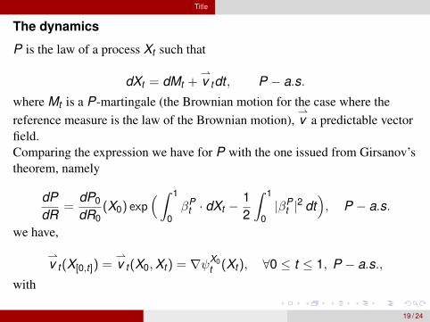
The dynamics
P is the law of a process Xt such that
dXt = dMt +v tdt , P − a.s.
where Mt is a P-martingale (the Brownian motion for the case where thereference measure is the law of the Brownian motion),
v a predictable vector
field.Comparing the expression we have for P with the one issued from Girsanov’stheorem, namely
dPdR
=dP0
dR0(X0) exp
(∫ 1
0βP
t · dXt −12
∫ 1
0|βP
t |2 dt), P − a.s.
we have,
v t (X[0,t]) =
v t (X0,Xt ) = ∇ψX0
t (Xt ), ∀0 ≤ t ≤ 1, P − a.s.,
with
ψx (t , z) := log ER
[exp
(η(x ,X1)+
∑s∈S,s>t
θs(Xs)+
∫T∩(t ,1]
p(r ,Xr ) dr) ∣∣∣Xt = z
], Rt−a.s.
19 / 24
Title
ψx (t , z) := log ER
[exp
(η(x ,X1) +
∑s∈S,s>t
θs(Xs)
+
∫T∩(t ,1]
p(r ,Xr ) dr) ∣∣∣Xt = z
], Rt − a.s.
Note that for t = 1, we have ψx (1, ·) = η(x , ·). Furthermore ψx is thesolution of the Hamilton-Jacobi-Bellman equation
[(∂t + ν∆)ψ +
12|∇ψ|2 + p
](t , z) = 0, 0 ≤ t < 1, t 6∈ S, z ∈ X ,
ψ(t , ·)− ψ(t−, ·) = −θ(t , ·), t ∈ S,
ψ(1, ·) = η(x , ·), t = 1.
20 / 24
Title
The forward velocity satisfies the equation
(∂t +v
x· ∇)(
v
x) = −ν∆(
v
x)−∇p, t < 1, t 6∈ S,
v
xt −
v
xt− = −∇θt , t ∈ S
v
x1 = ∇yη(x , ·), t = 1
(notice the “wrong sign")
21 / 24
Title
The backward velocity of P(·|X1 = y) solves
(∂t +v
y· ∇)(
v
y) = ν∆(
v
y)−∇p, t > 0, t 6∈ S,
v→,yt − v←,yt− = ∇θt , t ∈ S
v←,y0 = ∇yη(·, y), t = 0
Moreoverv
yt = ∇ϕy
t (z), t 6∈ S, with
(∂t − ν∆)ϕ+12|∇ϕ|2 + p = 0, t > 0, t 6∈ S
ϕ(t , ·)− ϕ(t−, ·) = θ(t , ·), t ∈ S,
ϕ(0, ·) = −η(·, y), t = 0.
22 / 24
Title
Remarks.
1. The current velocity vt = 12(v t +
v t ) solves the continuity equation
∂tµt +∇.(µtvt ) = 0
2. t → P0,t = (X0,Xt )∗P , probability measure on T2 is a relaxation of theLagrangian paths gt (·).
3. The pressure and the potentials θ do not depend on the final position, onlyon the actual position.
23 / 24
Title
The general solution of our generalization of Brenier’s type problemcan be described by
P =
∫X
P(·|X1 = y)
(corresponding to the gradient drift field v←,y = ∇ϕy ) but the averagebackward velocity
v t (z) =
∫∇z ϕ
yt (z) P tz
1 (dy)
P tz1 := P(X1 ∈ dy |Xt = z), is not a gradient, due to the nonlinearity of
the equations.This superposition phenomenon is reminiscent of Brenier’s multiphasevortex sheets model.
Final remark: This problem can be regarded as an infinite-dimensionalversion of a Schrödinger problem.
24 / 24
References
M. Arnaudon, A.B.C., Lagrangian Navier-Stokes diffusions onmanifolds: variational principle and stability, Bull. Sci. Math., 2012.
M. Arnaudon, A.B.C., C. Léonard, J.-C. Zambrini, An entropicinterpolation problem for incompressible viscid fluids, Ann. Inst. H.Poincaré Probab. Statist., 2020.