A Strategic Ideological Vote Raymond M. Duch raymond.duch@nuffield.ox.ac.uk Nuffield College University of Oxford 0X1 1NF Oxford UK Jeff May [email protected]Department of Political Science University of Houston Houston, TX 77204-3011 David A. Armstrong II [email protected]University of Oxford Dept of Politics and International Relations Manor Road Oxford OX1 3UQ * December 11, 2008 * Prepared for presentation at the Political Science and Political Economy Conference on ”Designing Demo- cratic Institutions”, London School of Economics. May 13-14, 2008 1
University of OxfordDept of Politics and International Relations
Manor RoadOxford OX1 3UQ
∗
December 11, 2008
∗Prepared for presentation at the Political Science and Political Economy Conference on ”Designing Demo-cratic Institutions”, London School of Economics. May 13-14, 2008
1
2
Abstract
Ideology is widely considered to be an important factor in shaping policy outcomes
and in influencing election outcomes. This essay confirms the importance of ideology in
explaining vote choice, based on 245 voter preference surveys world wide, from 30 countries,
and over a 25 year period. We also demonstrate, though, that the importance of ideology
in the vote function varies quite significantly across countries and, within countries, over
time. We propose a theory of the strategic ideological vote to explain this variation. The
argument suggests voters anticipate the post-election bargains negotiated amongst members
of the governing coalition and these anticipated policy agreements inform their vote choice.
Our analysis confirms that voters exercise a strategic ideological vote and that it frequently
differs from what would be predicted using sincere ideological voting models.
3
“However, many Danes are now worried by the power of the People’s party and
the racist attitudes of some of its supporters. Mr. Khader hopes to win votes by
promising to rebalance politics, with his own party acting as the fulcrum. “Blok
politik is not Danish,” he says. “The majority should be around the centre. The
veto power must be taken away from the People’s party.”
1 Introduction
This description of the 2007 Danish election illustrates a pervasive phenomenon in countries
with coalition governments: strategic ideological voting. In this particular case, Mr. Khader’s
New Alliance party gained considerable support from voters who favored the centre-right coali-
tion but were concerned that the conservative influence of the People’s Party over coalition
policy (immigration policy in particular) needed to be counter-balanced in a more centrist
direction. It became quite clear early in the campaign that New Alliance had a very high
probability of entering a post-election cabinet that would be lead by the centre-right Venstre
party (FT November 13, 2007, page 16; FT November 7, 2007, page 8). Accordingly, voters who
wanted to shift the governing coalition’s policy position in a more centrist direction, particularly
on immigration policy, had an incentive to vote strategically – for example abandoning their
sincere preference for the centre-right Venstre in favor of the New Alliance which would ensure
a government with a more centrist policy agenda.
The Danish example illustrates two features of the vote calculus that are pervasive in demo-
cratic contexts: First, vote choice conforms to a variant of the classic Downsian model (Downs
1957) in which voters locate themselves and candidates in a salient issue space and make choices
based on their proximity to the issue positions of competing candidates (Enelow and Hinich
1994). And second, the left-right ideological continuum is arguably the most important policy
dimension shaping vote choice. These observations build on a literature suggesting that ideology
plays a central role in contemporary democratic politics. There is overwhelming evidence that
the left-right continuum shapes party competition (Laver and Budge 1993, Budge and Robert-
son 1987, Huber and Inglehart 1995, Knutsen 1998, Adams et al. 2004); that it determines
4
legislative voting (Poole and Rosenthal 1997) and government spending priorities (Blais, Blake
and Dion 1993); and that it affects coalition outcomes (Warwick 1992, N.d.). Most importantly
we know that the ideological vote is important in certain countries (Kedar 2005, Adams, Merrill
and Grofman 2005, Merrill and Groffman 1999, Blais et al. 2001, Westholm 1997, Inglehart and
Klingemann 1976). Nevertheless, we do not have comparative evidence from a large number
of countries confirming our intuition about 1) the magnitude of the ideological vote; and 2)
the pervasiveness of ideological voting across democratic contexts. We propose to address this
lacuna in this essay.
The Danish example above raises a second interesting theoretical and empirical question re-
garding the ideological vote: If voters are behaving in a rational instrumental fashion, ideological
voting of a proximate kind should not be pervasive – voters in some contexts should strategically
abandon the parties to which they are ideologically proximate. And since we know that these
strategic incentives are strong in some contexts and non-existent in others, the magnitude of
the proximate ideological vote should vary across contexts. A second major contribution of this
essay is to demonstrate, based on a large number of cases, considerable contextual variation in
sincere ideological voting.
Our expectation is that the proximate ideological vote varies considerably across contexts
because features of these different contexts lead instrumentally rational voters to condition
their ideological vote on the coalitions, and their ideological compromises, that form after an
election. And we have evidence of contextual variation in the importance of ideology for political
behavior (Inglehart and Klingemann 1976). More recently, scholars have explored institutional
explanations for this variation. Kedar (2005), in particular, finds that voters in contexts with
coalition governments engage in compensational voting, i.e., certain voters will vote for more
extreme parties with the goal of shifting the policy position of governing coalitions closer to their
ideal points. And there have been recent findings in individual countries suggesting that voters
do respond in an instrumentally rational fashion to the strategic incentives associated with post-
election coalition formation possibilities – Gschwend (2007), Bowler and Karp (2006), Blais and
Levine (2006). Similarly, there is evidence that voters engage in vote discounting whereby
voters support more extreme candidates because they anticipate the moderating impact of the
5
legislative process on policy outcomes Tomz and Houweling (2007), Adams, Bishin and Dow
(2004), Merrill and Groffman (1999), Alesina and Rosenthal (1995). The third contribution of
this essay is to 1) propose a theory of the strategic ideological vote that builds on these recent
contributions; and 2) test empirically these theoretical propositions with a unique data base
that includes 245 voter preference studies.
We begin with a theory of the ideological vote that suggests how voters condition their
ideological vote on strategic incentives associated with coalition formation after the election
results are announced. The second part of the essay describes how we empirically estimate the
strategic ideological vote. We then summarize the results of our estimation: first comparing
estimates of sincere versus strategic ideological voting; and then comparing our strategic ideo-
logical estimates with those generated by discounting and directional models of the ideological
vote.
2 Theory
Our theoretical point of departure is Down’s (1957) notion that individuals make vote choices
based on their comparison of expected utilities for each of the competing parties. Voters are
instrumentally rational which implies that voters are motivated to select parties that are ideo-
logically proximate. This translates into the the conventional characterization of the ideological
vote in terms of Euclidean distance,
u(ji) = U − (xi − pj)2 (1)
where xi represents the ideological position of voter i and pj represents the ideological position
of party j and U is the upper bounds of (xi − pj)2 to ensure the lower bound of utility is zero
and the utility is positive. A smaller Euclidean distance translates into more utility and hence
contributes to the likelihood that a voter would vote for that party. This is what we characterize
as sincere ideological voting. If all voters adopt this proximate ideological voting decision rule,
we would find homogeneity in the importance of ideology in explaining vote choice across all
democratic contexts. And we entertain this possibility that the ideological vote is similar across
6
political contexts; think of this as a our null hypothesis.
But of course this simplicity is rarely the case. Downs (1957, 146) points out that one of the
factors complicating the voter’s decision calculus is coalition governments. Since rational voters
should only look upon elections as a means for selecting governments they should anticipate the
likely policy compromises that are negotiated after the election and they should cast a vote that
will ensure a coalition policy outcome that is most proximate to their ideal point. Downs (1957)
in fact was less than sanguine about the average voters ability to undertake these calculations
(Downs 1957, 256). If voters in coalition contexts ignore these second-order strategic consider-
ations, they effectively invite serious agency loss because parties have weakened incentives to
respond to voter preferences. Our intuition here is that Downs may have underestimated the
typical voter.
In these coalition contexts, coalitions form after elections as a result of bargain amongst
parties over the policies to be enacted by the government (Austen-Smith and Banks 1988, Pers-
son and Tabellini 2000). Policy outcomes in coalition government reflect the policy preferences
of the parties forming the governing coalition weighted by their legislative seats (Indridason
2007, Duch and Stevenson 2008).1 We believe that in coalition contexts voters anticipate these
policy outcomes and they use these to condition their ideological vote calculus represented
in Equation 1.2 Strategic voters, concerned with final policy outcomes (as opposed to party
platforms), condition their vote choices on coalition bargaining outcomes that occur after the
election(Austen-Smith and Banks 1988). In multiparty contexts with coalition governments,
Austen-Smith and Banks (1988) argue, sincere ideological voting is not rational. The implica-
tion of the Austen-Smith and Banks (1988) insight here is that the link between ideology and
vote choice is conditioned by rational voters engaging in strategic voting. Voters anticipate the1An alternative, and in our view less plausible, perspective is that the policy outcomes adopted in multiparty
contexts reflect the weighted preferences of all parties elected to the legislature (Ortuno-Ortin 1997, De Sinopoliand Iannantuoni 2007). This of course significantly reduces the second-order strategic incentives for voters.
2This anticipation of post-election policy compromises is not restricted to multiparty coalition contexts.Alesina and Rosenthal (1995), for example, suggest that voters in the U.S. context exercise a policy balanc-ing vote, anticipating the policy differences between Congress and the President. Kedar (2006) makes a moregeneral claim suggesting that this occurs in all Presidential regimes. Adams, Bishin and Dow (2004) analyzeindividual and aggregate-level data related to U.S. Senate elections and find support for the argument that vot-ers anticipate the moderating effect of the legislative process and hence vote for candidates with more extremepositions. Although they are careful to point out that their data could not distinguish this discounting argumentfrom a directional voting explanation.
7
likely coalition formation negotiations that occur after the election and they condition their
vote choices accordingly in order to maximize the likelihood that a coalition government forms
that best represents their policy preferences.
These formal statements that link coalition outcomes and vote choice present a challenge:
How do we precisely characterize this voter calculus that anticipates coalition outcomes after
the election? Grofman (1985) proposed a modification to the proximate ideological model that
takes into consideration what politicians are actually able to accomplish after an election. Voters
in the Grofman (1985) discounting model anticipate that candidates, if elected, will be able to
move policy only part way from the status quo position to their bliss point. This intermediate
distance between the candidates ideal point and the status quo is determined by a common
discounting factor shared by all voters. Hence, rather than the voters assessing the Euclidean
distance between their ideal point and pj in Equation 1, they employ a discounted version of pj ,
i.e., pj ∗ d where d varies between 0 and 1. When d = 1 we have a simple proximate ideological
model and when d approaches 0, Euclidean distance does not matter.
A related line of reasoning regarding the vote calculus suggests that voters focus on the
direction of policy movement. Voters in these directional models of ideological voting implicitly
understand that there is a status quo bias in the post election policy making process. Hence, as
Matthews (1979) argues, voters prefer candidates who move policy from the status quo toward
their ideal point. In a uni-dimensional policy world where left-right self identification is the
only policy dimension determining vote choice, the candidate’s location relative to the status
quo point is the only consideration that matters to voters – intensity does not come into play.
Rabinowitz and Macdonald (1989) explicitly add intensity to their directional model of vote
choice. The voter utility function is a scalar or dot product of the vectors representing the
policy positions of voters (V) and candidates (C): U(V,C) = V ·C =∑n
i=1 vici. If we assume
that vote choice is determined by a single left-right ideology dimension then the vote utility is
simply the product of the voter and candidate’s ideal points, both calculated relative to the
neutral point. Take the case where there are two conservative parties located to the right of the
neutral point on a left-right continuum. Voters to the right of the neutral point will give all of
their votes to the conservative party with the most extreme location to the right of the neutral
8
point – the other conservative party would receive none of the votes of voters to the right of
the neutral point.
Adams, Merrill and Grofman (2005) and Merrill and Groffman (1999) convincingly argue
that voters employ mixed strategies of discounted and directional voting that likely vary by
context. Clearly voters are conditioning their ideological vote on their expectations regarding
post-election policy outcomes. But the nature of voter expectations in both the directional and
discounting models resembles a relatively naive heuristic: Voters anticipate political and institu-
tional resistance to changing the status quo and therefore vote for parties that are ”directionally
proximate” but have more extreme ideal points.
Voter reasoning may be somewhat more informed than simply discounting or voting direc-
tionally; they may be reasonably well-informed about post-election coalition formation outcomes
and this may condition the ideological vote. Kedar (2005) argues that the rational voter focuses
on policy outcomes and hence on the issue positions that are ultimately adopted by the coalition
government that forms after an election. And she demonstrates that in political systems with
coalition governments this leads to “compensational voting”, rather than ideological proximity
voting, aimed at minimizing the policy distance between the policy compromises negotiated by
the governing coalition and the voters ideal policy position.
Duch and Stevenson (2008) develop a contextual theory of economic voting in which voters
anticipate the likely coalitions that form after an election and they assess the impact of their
vote choice on the likelihood of different coalitions coming to power after an election. And this
information is used by instrumentally rational voters to weight the importance of an economic
competency signal in their vote choice function. Hence, parties that are certain to enter a
governing coalition (i.e., perennial coalition partners) should, all things being equal, get no
economic vote since a vote for this party has no impact on the coalition that ultimately forms.
Both Kedar (2005) and Duch and Stevenson (2008) go to considerable length to formalize how
post-election coalition formation enters into the vote choice function. Building on these works,
we propose a model of the ideological vote in which voters anticipate the coalitions that form
after the election – what we call the strategic ideological vote.
To capture the impact of this post-election coalition formation bargaining on the ideolog-
9
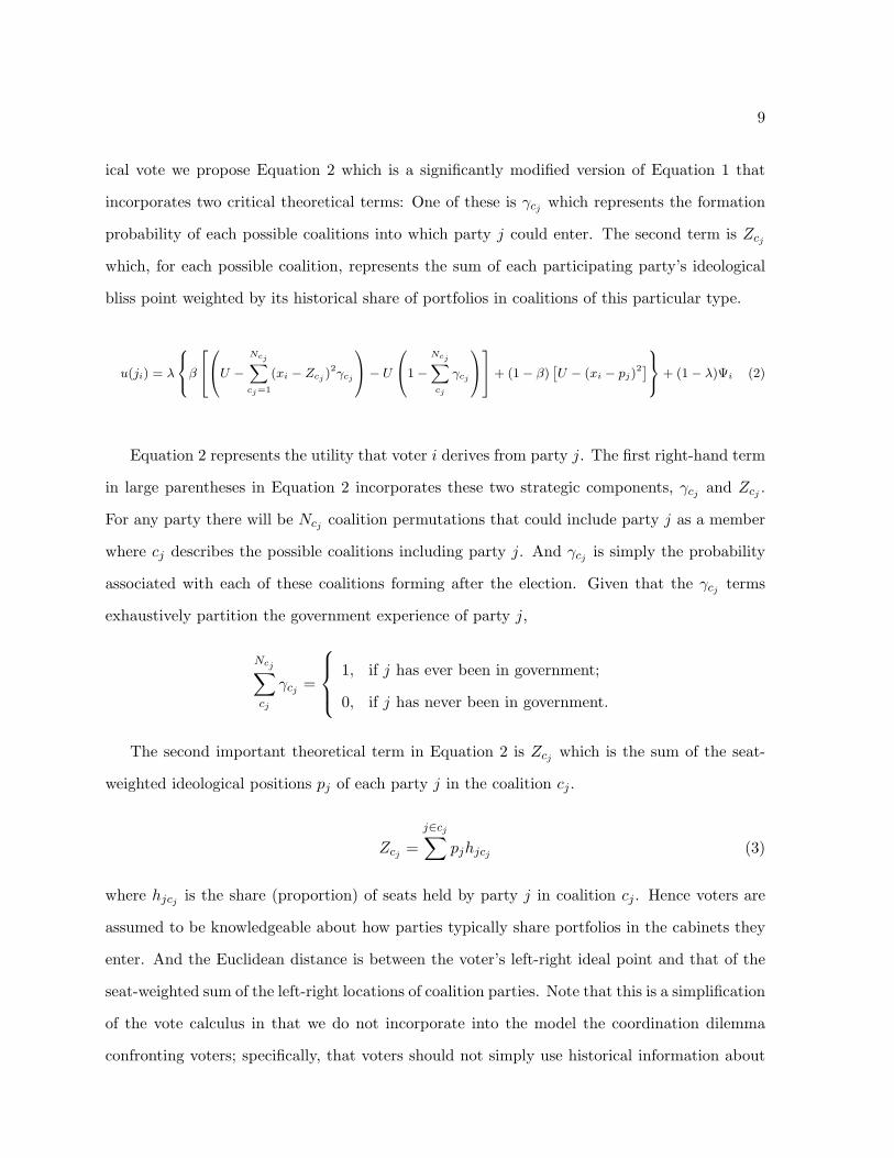
ical vote we propose Equation 2 which is a significantly modified version of Equation 1 that
incorporates two critical theoretical terms: One of these is γcj which represents the formation
probability of each possible coalitions into which party j could enter. The second term is Zcj
which, for each possible coalition, represents the sum of each participating party’s ideological
bliss point weighted by its historical share of portfolios in coalitions of this particular type.
u(ji) = λ
βU −
Ncj∑cj=1
(xi − Zcj )2γcj
− U
1−Ncj∑cj
γcj
+ (1 − β)[U − (xi − pj)2
]+ (1 − λ)Ψi (2)
Equation 2 represents the utility that voter i derives from party j. The first right-hand term
in large parentheses in Equation 2 incorporates these two strategic components, γcj and Zcj .
For any party there will be Ncj coalition permutations that could include party j as a member
where cj describes the possible coalitions including party j. And γcj is simply the probability
associated with each of these coalitions forming after the election. Given that the γcj terms
exhaustively partition the government experience of party j,
Ncj∑cj
γcj =
1, if j has ever been in government;
0, if j has never been in government.
The second important theoretical term in Equation 2 is Zcj which is the sum of the seat-
weighted ideological positions pj of each party j in the coalition cj .
Zcj =j∈cj∑
pjhjcj (3)
where hjcj is the share (proportion) of seats held by party j in coalition cj . Hence voters are
assumed to be knowledgeable about how parties typically share portfolios in the cabinets they
enter. And the Euclidean distance is between the voter’s left-right ideal point and that of the
seat-weighted sum of the left-right locations of coalition parties. Note that this is a simplification
of the vote calculus in that we do not incorporate into the model the coordination dilemma
confronting voters; specifically, that voters should not simply use historical information about
10
coalition formation but also anticipate how other voters will use this information about post-
election coalition bargaining. Voters in these models anticipate how the strategic ideological
vote of other voters will affect post-election coalition outcomes and vote accordingly (McCuen
and Morton (2000) is one of the few efforts to our knowledge that addresses the modeling
challenges posed by such behavior).
To ensure that parties with no governing experience,∑Ncj
cj γcj = 0, gain no utility from the
strategic part of the model, we subtract U(
1−∑Ncj
cj γcj
). This acts as a switch that makes
β [. . .] = 0 in Equation 2, for parties with no governing experience. Finally, note that the full
strategic component of the model that falls within the square brackets is weighted by β which
indicates the importance of strategic considerations and is assumed to vary between 0 and 1.
Equation 2 also includes the sincere ideological expression that we saw earlier in Equation
1. Note that this “expressive” Euclidean distance term is weighted by 1 − β. As β gets large,
i.e., voters put more weight on strategic ideological considerations, this expressive component
of the ideological vote gets smaller. Hence voters in this model can give varying weight to
ideological considerations that are entirely expressive (or sincere) which is captured by the
standard Euclidean distance term weighted by 1− β.
The decision to vote for a particular political party is of course not simply guided by the
voter’s perceived left-right spatial distance from the party. Accordingly, we include in Ψi to
control for the range of other factors that typical enter into a voter utility function.3 We add a
λ term, that varies from 0 to 1 which represents the weight of the ideological vote overall (both
strategic and sincere) in the voter preference function. This implies that the relative importance
of other factors, Ψi, in the vote utility function is captured by the weight 1− λ.
The voter utility function sketched out in Equation 2 is a precise statement of how ideology
enters into the voter preference function: Voters in this model can give varying weight to
ideological considerations that are entirely expressive (or sincere) which is captured by the
standard Euclidean distance term weighted by 1−β. On the other hand, a large β term implies3The inclusion of Ψi here makes sense on both theoretical and methodological grounds (see Adams, Merrill
and Grofman (2005) who make a strong case for the inclusion of such non-policy variables in spatial models ofvote choice). The Ψi is a vector of factors that varies by individual, but not across parties. Further, the effectsof these variables within country do not vary either by party or by individual.
11
that voters condition their ideological vote on strategic considerations related to post-election
coalition formations. We suggest that there are two key elements to this strategic calculus: γcj
which represents the probability of each possible coalitions into which party j could enter; and
Zcj which represents the sum of each participating party’s ideological bliss point weighted by
its historical share of portfolios in coalitions of this particular type. Finally, the vote utility
function includes the host of other non-ideological factors, Ψi, that enter into the vote calculus –
the importance of these factors in vote choice, relative to ideological considerations, is captured
by the 1−λ term. Our theory suggests that, in general, ideology matters for vote choice; hence
λ for some important number of cases is non-zero. It also suggests that there are contexts in
which the strategic components of our model have a significant impact on the vote calculus –
that β is non-zero in many contexts and that we have correctly captured the strategic calculus
with the two terms Zcj and γcj . We now turn to these empirical efforts in the next section.
The γcj term in Equation 2 represents the likelihood of different possible coalitions forming
with party j. We assume that voters know the historical frequency with which all possible
governing coalitions have occurred. Hence, when a party that has no chance of participating in
a post-election government, i.e., γcj = 0 (for cj = 1, 2, ..., Ncj ) its ideological voting is entirely
sincere and therefore determined by the weight (1−β).4 (1−β) captures the utility that voters
get from simply expressing an ideological preference for a political party.
Note that when β is zero or when all the elements of γcj = 0, we get the same result –
proximity voting. There is a subtle difference though: If in fact β is zero then no parties should
receive a second-order strategic ideological vote. The situation when γcj = 0 for cj = 1, 2, ..., Ncj
implies a different set of outcomes. Clearly for a subset of our sampled countries, there will be
some parties for whom γcj = 0 (no chance of participating in a governing coalition) and hence
4Meffert and Gschwend (2007a) speculate that median voters might support extreme parties in order to forcemajor parties, more proximate to the median voter, into a coalition government. This is motivated by concernsother than ideology though – it seems more motivated by a taste for grand coalitions – and in fact generatesexactly the opposite prediction to the one in our model.
12
the ideological vote they receive will be entirely expressive. But in any political system with
multi-party governing coalitions there will be at least two parties with a non-zero probability
of participating in the governing coalition i.e., (γcj > 0 for some combination of parties j) and
this should make it possible to distinguish empirically between whether the absence of strategic
ideological voting is the result of β = 0 or γcj = 0 for all combinations of j.
Voters use this historical information regarding participation in governing coalitions to es-
tablish the probabilities that parties will participate in the government after an election. Hence,
we assume that voters are knowledgeable about γcj , i.e., the likelihoods of different combinations
of parties making up the governing coalition that forms after an election. And there is evidence
to suggest in fact that they are quite knowledgeable about these probabilities (Bargsted and
Kedar 2007, Duch and Stevenson 2008, Irwin and van Holsteyn 2003).
The hjcj term in Equation 2 represents party j′s share of the portfolios in a governing
coalition – what we have labeled administrative responsibility. Voters are informed about the
likely contribution of each party to governing coalitions into which the party typically enters.5
Hence, for example, voters know that the People’s Party for Freedom and Democracy (VVD)
in the Netherlands typically commands about 65 percent of the portfolios when it enters a
governing coalition with the Christian Democratic Appeal (CDA). This is important in our
theory because shares of portfolios essentially determine the contribution of each governing
party to the government’s policy positions. The left-right policy compromise amongst the
coalition partners (Zcj ) is determined by the sum of their ideological positions weighted by each
party’s share of the cabinet portfolios. This “contribution” of a party’s left-right position to
the coalition compromise on the left-right continuum will affect the size of its ideological vote.
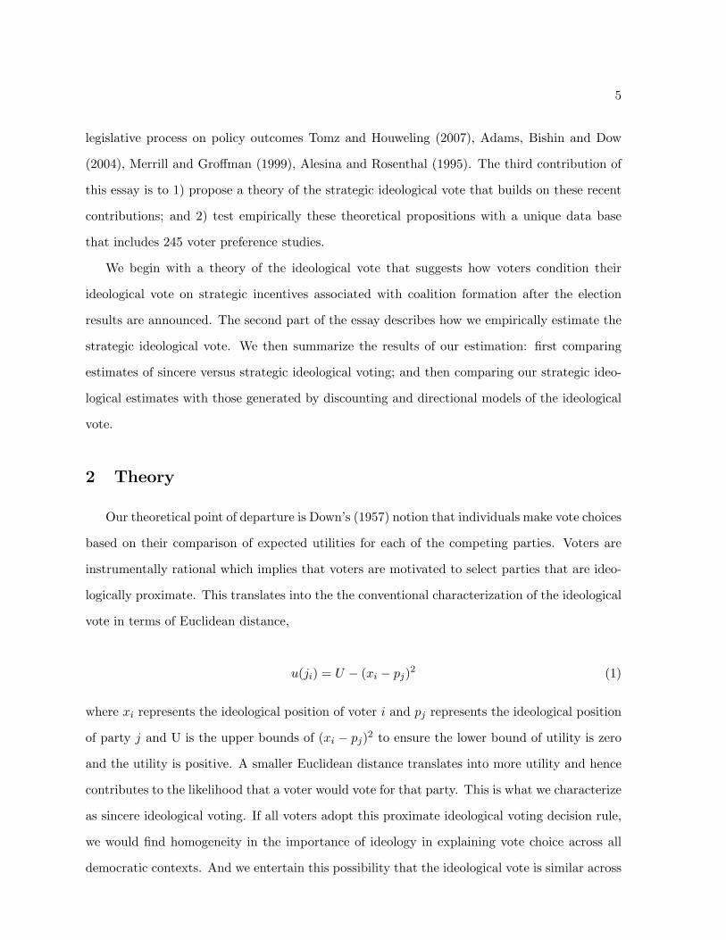
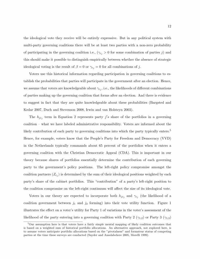
Voters in our theory are expected to incorporate both hjcj and γcj (the likelihood of a
coalition government between j1 and j2 forming) into their vote utility function. Figure 1
illustrates the effect on a voter’s utility for Party 1 of variations in the voter’s assessment of the
likelihood of the party entering into a governing coalition with Party 2 (γ1,2) or Party 3 (γ1,3)
5Our assumption here is that voters have a fairly simple mental mapping of likely coalition outcomes thatis based on a weighted sum of historical portfolio allocations. An alternative approach, not explored here, isto assume voters anticipate portfolio allocations based on the ”pivotalness” and formateur status of competingparties at the time these surveys are conducted (Snyder and Ansolabehere 2005, Morelli 1999).
13
and variations in j2 and j3’s share of cabinet portfolios. These two variables have interactive
effects on the voter’s utility – for example, if Party 2 has a very small expected share of the
cabinet portfolios then the impact of variations in γ1,2 on the voter’s utility for Party 1 will
likely be quite small.
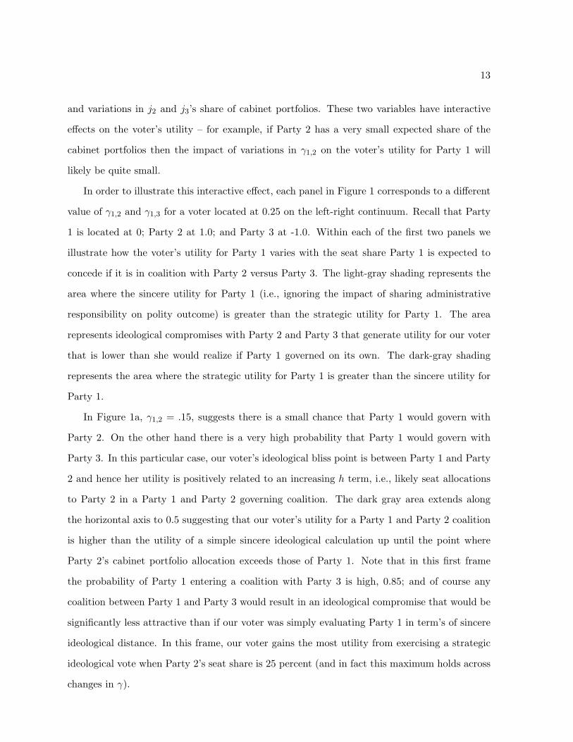
In order to illustrate this interactive effect, each panel in Figure 1 corresponds to a different
value of γ1,2 and γ1,3 for a voter located at 0.25 on the left-right continuum. Recall that Party
1 is located at 0; Party 2 at 1.0; and Party 3 at -1.0. Within each of the first two panels we
illustrate how the voter’s utility for Party 1 varies with the seat share Party 1 is expected to
concede if it is in coalition with Party 2 versus Party 3. The light-gray shading represents the
area where the sincere utility for Party 1 (i.e., ignoring the impact of sharing administrative
responsibility on polity outcome) is greater than the strategic utility for Party 1. The area
represents ideological compromises with Party 2 and Party 3 that generate utility for our voter
that is lower than she would realize if Party 1 governed on its own. The dark-gray shading
represents the area where the strategic utility for Party 1 is greater than the sincere utility for
Party 1.
In Figure 1a, γ1,2 = .15, suggests there is a small chance that Party 1 would govern with
Party 2. On the other hand there is a very high probability that Party 1 would govern with
Party 3. In this particular case, our voter’s ideological bliss point is between Party 1 and Party
2 and hence her utility is positively related to an increasing h term, i.e., likely seat allocations
to Party 2 in a Party 1 and Party 2 governing coalition. The dark gray area extends along
the horizontal axis to 0.5 suggesting that our voter’s utility for a Party 1 and Party 2 coalition
is higher than the utility of a simple sincere ideological calculation up until the point where
Party 2’s cabinet portfolio allocation exceeds those of Party 1. Note that in this first frame
the probability of Party 1 entering a coalition with Party 3 is high, 0.85; and of course any
coalition between Party 1 and Party 3 would result in an ideological compromise that would be
significantly less attractive than if our voter was simply evaluating Party 1 in term’s of sincere
ideological distance. In this frame, our voter gains the most utility from exercising a strategic
ideological vote when Party 2’s seat share is 25 percent (and in fact this maximum holds across
changes in γ).
14
Figure 1: Utility for Party 1 as γ1,2, γ13, h212and h213 Change∗
Seat Shares of Party 2 in Coalition with Party 1
Sea
t Sha
res
of P
arty
3 in
Coa
litio
n w
ith P
arty
1
0.0 0.2 0.4 0.6 0.8 1.0
0.00
0.25
0.50
0.75
1.00
(a) γ12 = .15, γ13 = .85, x = 0.25
Seat Shares of Party 2 in Coalition with Party 1
Sea
t Sha
res
of P
arty
3 in
Coa
litio
n w
ith P
arty
1
0.0 0.2 0.4 0.6 0.8 1.0
0.0
0.2
0.4
0.6
0.8
1.0
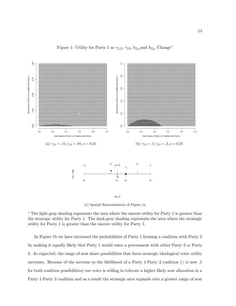
(b) γ12 = .5, γ13 = .5, x = 0.25
c(0, 1)
c(1,
1.3
5)
−1 p1 == 0 1
p2p3
x
●
z13 ' z12
'
z13 z12
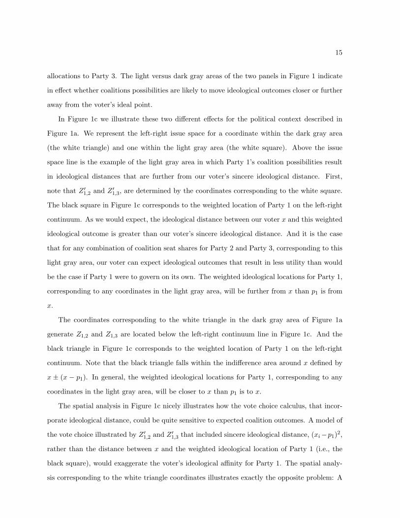
(c) Spatial Representation of Figure 1a
∗ The light-gray shading represents the area where the sincere utility for Party 1 is greater thanthe strategic utility for Party 1. The dark-gray shading represents the area where the strategicutility for Party 1 is greater than the sincere utility for Party 1.
In Figure 1b we have increased the probabilities of Party 1 forming a coalition with Party 2
by making it equally likely that Party 1 would enter a government with either Party 2 or Party
3. As expected, the range of seat share possibilities that favor strategic ideological voter utility
increases. Because of the increase in the likelihood of a Party 1-Party 2 coalition (γ is now .5
for both coalition possibilities) our voter is willing to tolerate a higher likely seat allocation in a
Party 1-Party 3 coalition and as a result the strategic area expands over a greater range of seat
15
allocations to Party 3. The light versus dark gray areas of the two panels in Figure 1 indicate
in effect whether coalitions possibilities are likely to move ideological outcomes closer or further
away from the voter’s ideal point.
In Figure 1c we illustrate these two different effects for the political context described in
Figure 1a. We represent the left-right issue space for a coordinate within the dark gray area
(the white triangle) and one within the light gray area (the white square). Above the issue
space line is the example of the light gray area in which Party 1’s coalition possibilities result
in ideological distances that are further from our voter’s sincere ideological distance. First,
note that Z ′1,2 and Z ′1,3, are determined by the coordinates corresponding to the white square.
The black square in Figure 1c corresponds to the weighted location of Party 1 on the left-right
continuum. As we would expect, the ideological distance between our voter x and this weighted
ideological outcome is greater than our voter’s sincere ideological distance. And it is the case
that for any combination of coalition seat shares for Party 2 and Party 3, corresponding to this
light gray area, our voter can expect ideological outcomes that result in less utility than would
be the case if Party 1 were to govern on its own. The weighted ideological locations for Party 1,
corresponding to any coordinates in the light gray area, will be further from x than p1 is from
x.
The coordinates corresponding to the white triangle in the dark gray area of Figure 1a
generate Z1,2 and Z1,3 are located below the left-right continuum line in Figure 1c. And the
black triangle in Figure 1c corresponds to the weighted location of Party 1 on the left-right
continuum. Note that the black triangle falls within the indifference area around x defined by
x ± (x − p1). In general, the weighted ideological locations for Party 1, corresponding to any
coordinates in the light gray area, will be closer to x than p1 is to x.
The spatial analysis in Figure 1c nicely illustrates how the vote choice calculus, that incor-
porate ideological distance, could be quite sensitive to expected coalition outcomes. A model of
the vote choice illustrated by Z ′1,2 and Z ′1,3 that included sincere ideological distance, (xi−p1)2,
rather than the distance between x and the weighted ideological location of Party 1 (i.e., the
black square), would exaggerate the voter’s ideological affinity for Party 1. The spatial analy-
sis corresponding to the white triangle coordinates illustrates exactly the opposite problem: A
16
model of the vote choice illustrated by Z1,2 and Z1,3 that included sincere ideological distance,
(xi − p1)2, rather than the distance between x and the weighted ideological location of Party 1
(i.e., the black triangle), would underestimate the voter’s ideological affinity for Party 1. And
this underestimation or overestimation of ideological outcomes can lead to an inaccurate rep-
resentation of the vote choice calculus and an incorrectly predicted ideological vote, although
this depends on where the other parties and their likely coalition partners were located in the
issue space.
Our ability to empirically distinguish between the sincere and strategic ideological models
requires that voters and parties locate themselves such that strategic and sincere predictions
are quite distinct. Whether these strategic incentives materialize in any particular context or
for any group of political parties of course depends on the coalition history of parties and the
location of parties and voters in the ideological space. We can see this by referring back to
Figure 1c. The ideological distance between x and p1 is actually quite a bit smaller than the
distance between x and the weighted ideological outcome. But this may have no consequences
for x’s vote choice. Lets assume the weighted ideological outcomes associated with all other
coalition possibilities fell somewhere outside of the space between the black box square and
x. In this case calculating ideological distance sincerely or strategically will result in the same
vote choice since both result in a vote choice for Party 1. Moreover, it will frequently be
the case that the vote choices predicted by the sincere and strategic models will be identical.
Hence, the conditions for the separating equilibria are actually quite restrictive. Nevertheless,
our expectation is that there are sufficiently numerous cases in which the strategic incentives
dictate a vote choice distinct from that predicted by a sincere ideological model and hence
we expect to see the net superiority of the strategic model when we compare the two model
predictions over a large number of parties and political contexts. Note though that it is virtually
impossible to assess these two models in a rigorous fashion without a large number of cases.
Hence, drawing conclusions about how ideology shapes vote choice based on a small number of
cases is almost certainly to result in misleading conclusions.
17
2.2 Empirical implications of the strategic ideological vote model
Any effort to empirically test our theoretical claims about how ideology shapes vote choice
must include observations that vary over xi, pj , γc, and hjcj . The first two requirements are
quite standard: there needs to be variation in the self-placement of voters on the ideological
continuum and parties need to vary along this same continuum. The other requirements are
somewhat more demanding: parties need to vary considerably in terms of their probability
of participating in a governing coalition; and there needs to be variation across parties and
over time in the allocation of cabinet portfolios to different parties in the governing coalition.
Further, the functional form of the empirical model has to be specified such that it generates
estimates for the parameters β and λ. If any one of these is excluded from the empirical model
because of a deliberate model specification decision or because of insufficient variation then one
very likely will draw misleading conclusions about how ideology shapes vote choice.
One strategy for ensuring appropriate variation is through experimental treatments. Meffert
and Gschwend (2007b), for example, employ experiments to demonstrate that voters are capable
of making strategic voting decisions that anticipate post-election coalition formations and the
relative policy weights of parties in these coalitions. Tomz and Houweling (2007) implement an
online experiment demonstrating that voters can make sophisticated policy balancing decisions
as part of their vote choice and that this is particularly the case with centrist voters.6 The other
strategy is to estimate the model in Equation 2 using a large number of voter preference surveys
from countries with very different political and institutional contexts. This is the strategy we
adopt in this essay. But before moving to the empirics, we briefly explain what we can learn –
or not learn – about the parameters in Equation 2 from estimating this model of the ideological
vote in different national contexts.
Case 1: The Absence of an Ideological Vote (λ = 0). There may be political contexts in which
ideology does not shape, in any significant fashion, vote choice. Hence some of the contextual
variation in ideological voting may simply result from the fact that λ ≈ 0; in which case,
voter utility for a party is entirely accounted for by Ψi which are factors other than ideological
self-placement. Cases in which λ ≈ 0 have two important implications for our theory of the6Other experimental advances in this regard include Claassen (2007), Lacy and Paolino (2005).
18
strategic ideological vote. First, a non-zero λ term is a necessary condition for the existence
of strategic ideological voting. To the extent that our sample of contexts are overwhelmingly
dominated by cases in which λ ≈ 0, we would have little confidence in the existence of any kind
of ideological voting. Second, an under-specified model that does not include both the strategic
and sincere components of the ideological vote, plus the vector of control variables, Ψi, will
be unable to distinguish between cases where λ ≈ 0 (no ideological voting) versus those where
β > 0 (strategic ideological voting).
Case 2: Ideological voting in contexts with single-party governing coalitions (λ > 0) (β = 0)
(γ = 1). Note from Equation 2 that if γcj = 1 for cj = j we have the case in which party
j only serves in single-party governments. When this is the case, Equation 2 reduces to the
conventional proximity ideological vote expression in Equation 1. Hence our theory predicts that
parties with no coalition governing experience should receive a strong conventional proximate
ideological vote. These particular cases will not be very helpful empirically in distinguishing
between the relative importance of sincere versus strategic ideological contributions to vote
choice because the strategic component of the utility function is undefined for non-coalition
governing parties.
Case 3: Ideological voting for parties with no governing experience (λ > 0) (β = 0) (γ = 0).
Political parties that never participate in government are also predicted to receive no strategic
ideological vote. Again, for these parties the strategic component of Equation 2 reduces to zero
because (γ = 0) and hence only proximate ideological voting (along with non-ideological factors)
shapes vote choice. Because the strategic component of the utility function is undefined, these
cases provide no empirical leverage for distinguishing between the importance of the strategic
versus sincere ideological vote.
Case 4: Strategic ideological voting (λ > 0) (0 < γ < 1 β > 0). Finally, there are a group
of cases in our sample of party ideological votes that are particularly important for testing our
theoretical contention that the ideological vote is strategic. These are cases in which λ > 0,
i.e., ideology is important, in general, for vote choice, and where (0 < γ < 1), i.e., parties have
a history of serving in coalition governments. For these parties both the strategic and sincere
components of Equation 2 are defined and, at least in principle, we should be able to assess the
19
relative importance of these two theoretical terms.
The problem here is that we have relatively poor information for calibrating the magnitude
of β. First, a large number of contexts provide no information about the strategic component
of the ideological vote because, as we pointed out earlier, β = 0 by definition, i.e., there are
no opportunities for voters to exercise a strategic ideological vote. Second, even for those cases
in which there are opportunities to exercise a strategic ideological vote, the predictions from
a model in which β = 1 versus a model in which β = 0 will be identical for a large number
of voters. This frequently happens because, given the ideological self-placement of voters, the
optimal vote choice, taking into consideration post-election coalition compromises, is the same
as one that simply considered the ideological proximity of parties. This makes it difficult to
assess the independent contribution of the strategic and sincere components of Equation 2 by
simply estimating an empirical model that includes both terms.
While it is difficult to get a precise estimate of the magnitude of β, we can gain some insight
here by comparing two empirical model specifications: one with ideological distance represented
in its sincere form compared to a specification with ideology represented as a weighted strategic
term. Our hypothesis is that 1) ideological distance in its weighted strategic form will have a
more important impact, measured by the coefficient on the distance measure, on vote choice than
in its sincere form; and 2) the model with the strategic ideological specification will better predict
vote choice than the sincere specification. To the extent that both tests favour the strategic
ideological model, we can be reasonably confident that this is a better net representation of the
voter calculus in multi-party coalition contexts.
We have described the strategic ideological voter as being fully informed about the relative
electoral strengths of the parties; their likelihood of entering a governing coalition; their location
on a left-right continuum; and their likely portfolio allocation if they enter a governing coalition.
Equation 2 indicates how voters incorporate information about post election coalition formation
into their expected utility for a particular party. The empirical test of our theory is whether
these expected utilities generate better predicted vote choices than a sincere model of ideological
voting. The next section presents the results of this straight-forward empirical exercise.
20
3 Estimating the Strategic Ideological Vote
Our theory summarized in Equation 2 suggests that ideology enters the voter preference
function in some combination of strategic (β∑Ncj
cj=1(xi−Zcj )2γcj ) and sincere ((1−β)(xi−pj)2)
reasoning. Most empirical models of the ideological vote include the sincere component but
exclude the strategic component. Frequently this is of no consequence because the two terms
are highly correlated and in fact are identical in many contexts where there is a history of single
party governments. Our theoretical argument in favor of a strategic ideological vote 1) presumes
that there are in fact a large number of contexts in which these two terms are different; and
2) implies that in these cases the strategic representation of the ideological vote better predicts
vote choice. We now review the data employed to estimate the parameters in Equation 2.
In order to obtain reliable estimates of the parameters in Equation 2, our estimates are
based on data from 245 election studies. These include studies from a number of comparative
voting studies: from the Central and Eastern Euro-Barometer, Comparative Study of Electoral
Systems (CSES and CSES2), Euro-Barometer, Afro-Barometer, Latino-Barometer, and World
Values Survey. These cover 30 countries7 from the years 1981-2006. Each survey includes, at
a minimum: 1) the respondent’s intended vote (or reported vote for a handful of post-election
surveys); 2) the respondent’s left-right self-placement; and 3) the appropriate control variables
for estimating a vote choice model in each country.
We will estimate the underlying utility of respondents for each competing party by esti-
mating a conditional logit function with vote preference over competing political parties as the
dependent variable. The vote preference question in the surveys we analyze is typically of the
form, “if an election were held today which party would you vote for?”.
The vote choice questions differed in their relationship to the election for which the vote
applied: surveys conducted directly after elections simply ask respondents to report their vote
choice in the preceding election; surveys that were conducted just before an election ask respon-
dents for whom they intend to vote for in the upcoming election; and surveys that were not7Albania, Australia, Austria, Belgium, Bulgaria, Croatia, Czech Republic, Denmark, Estonia, Finland, France,
proximate to an election ask the voter about a hypothetical election (“If there were a general
election tomorrow, which party would you support?”).8 All the surveys we used allow the voter
to express whether they did not vote or do not intend to vote. Further, most allow the voter
to indicate if she cast (or intends to cast) a blank ballot. Where these studies differ is in how
they elicit the information that the respondent does not intend to vote. While this is a readily
apparent difference in the way the vote choice question is asked in different surveys, it is unlikely
to be consequential in our analysis, since (for other reasons) we decided to ignore non-voters in
our analysis.
The left-right self placement measure used for the Euclidean distance terms in Equation 2
is based on questions that were worded similarly to: “In political matters, people talk of ‘the
left’ and ‘the right’. How would you place your views on this scale? 1=Left 10=Right.” The
left-right scales were of different ranges across the surveys (some were 10-scale, others 7-scale,
etc.) but were all standardized to have mean zero and unit variance to facilitate comparisons
across surveys.9
Empirically, the more problematic element in the Euclidean term is the measure of party
placements, pj from Equation 2. We measure party placement with the mean of the left-right
placement of the voters for party j. Using this measure we were able to estimate ideological
distance for all of the voter preference studies in our sample. It also has the advantage of
avoiding endogeneity bias that some claim is associated with measures of party placement that
are based on respondents locating parties on the left-right ideological continuum (Macdonald
and Listhaug 2007, Merrill and Adams 2001).10
Only if we have accounted for all the important influences on the vote will we be confident
that our estimates reflect the true relationship between ideological self-placement and vote8The key question for our analysis is whether these differences introduce systematic biases into our estimates
of the strength of economic voting that will make them less comparable. Our analyses suggest that they do not.9A detailed description of the surveys and question wording of items used in the analysis is available on the
authors’ web site: www.raymondduch.com/ideologicalvote.10Rehm (2007) provides a detailed discussion of the merits and disadvantages of employing the constituency-
based strategy for estimating party positions, including comparisons with the other methods for locating par-ties in policy space. We replicate the results reported below using two other methods: party placements thatare the mean for all respondents identifying with each party; and party placements based on questions ask-ing respondents to locate parties in the ideological space. These methods generate essentially the same find-ings as those reported below. Results using these other two methods are available on the authors’ web page:www.raymondduch.com/ideologicalvote
22
choice in the population to which the relevant survey applies. Hence, our statistical models
for each survey include variables that are known to be important in voting in the particular
country and time – the Ψi term in Equation 2. We identify those variables from the literature on
comparative voting behavior and on the country specific literatures on voting in each country.11
It is the γcj and hjcj (through the Zcj term) in Equation 2 that distinguish strategic from
sincere representations of the ideological vote. The γcj represents the voter’s assessment of the
likelihood of all possible coalition permutations in which party j could participate. We employ
an historical approach to measuring voter beliefs about the likelihood of participating in each
possible coalition permutation. Specifically, we calculate, for each party (at the time of the
survey), the months since 1960 that the party has been in the cabinet and discounted versions
of this measure that gives more weight to more recent experience.
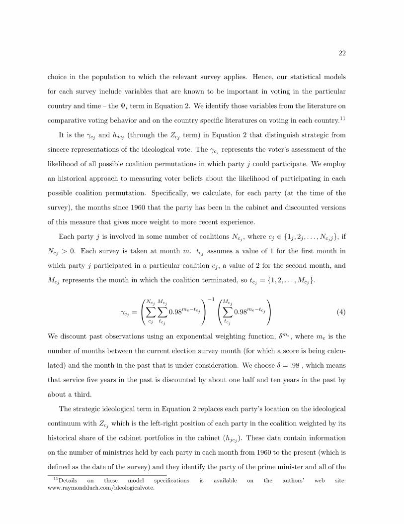
Each party j is involved in some number of coalitions Ncj , where cj ∈ {1j , 2j , . . . , Ncjj}, if
Ncj > 0. Each survey is taken at month m. tcj assumes a value of 1 for the first month in
which party j participated in a particular coalition cj , a value of 2 for the second month, and
Mcj represents the month in which the coalition terminated, so tcj = {1, 2, . . . ,Mcj}.
γcj =
Ncj∑cj
Mcj∑tcj
0.98me−tcj
−1Mcj∑tcj
0.98me−tcj
(4)
We discount past observations using an exponential weighting function, δme , where me is the
number of months between the current election survey month (for which a score is being calcu-
lated) and the month in the past that is under consideration. We choose δ = .98 , which means
that service five years in the past is discounted by about one half and ten years in the past by
about a third.
The strategic ideological term in Equation 2 replaces each party’s location on the ideological
continuum with Zcj which is the left-right position of each party in the coalition weighted by its
historical share of the cabinet portfolios in the cabinet (hjcj ). These data contain information
on the number of ministries held by each party in each month from 1960 to the present (which is
defined as the date of the survey) and they identify the party of the prime minister and all of the11Details on these model specifications is available on the authors’ web site:
www.raymondduch.com/ideologicalvote.
23
parties in the governing coalition. These data on cabinet portfolios were compiled by the authors
and a detailed description of the sources is available at www.raymondduch.com/ideologicalvote.
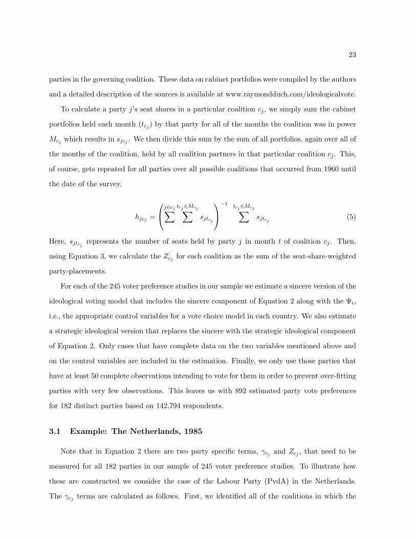
To calculate a party j’s seat shares in a particular coalition cj , we simply sum the cabinet
portfolios held each month (tcj ) by that party for all of the months the coalition was in power
Mcj which results in sjcj . We then divide this sum by the sum of all portfolios, again over all of
the months of the coalition, held by all coalition partners in that particular coalition cj . This,
of course, gets repeated for all parties over all possible coalitions that occurred from 1960 until
the date of the survey.
hjcj =
j∈cj∑ tcj∈Mcj∑sjtcj
−1 tcj∈Mcj∑sjtcj
(5)
Here, sjtcjrepresents the number of seats held by party j in month t of coalition cj . Then,
using Equation 3, we calculate the Zcj for each coalition as the sum of the seat-share-weighted
party-placements.
For each of the 245 voter preference studies in our sample we estimate a sincere version of the
ideological voting model that includes the sincere component of Equation 2 along with the Ψi,
i.e., the appropriate control variables for a vote choice model in each country. We also estimate
a strategic ideological version that replaces the sincere with the strategic ideological component
of Equation 2. Only cases that have complete data on the two variables mentioned above and
on the control variables are included in the estimation. Finally, we only use those parties that
have at least 50 complete observations intending to vote for them in order to prevent over-fitting
parties with very few observations. This leaves us with 892 estimated party vote preferences
for 182 distinct parties based on 142,794 respondents.
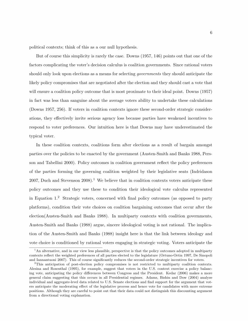
3.1 Example: The Netherlands, 1985
Note that in Equation 2 there are two party specific terms, γcj and Zcj , that need to be
measured for all 182 parties in our sample of 245 voter preference studies. To illustrate how
these are constructed we consider the case of the Labour Party (PvdA) in the Netherlands.
The γcj terms are calculated as follows. First, we identified all of the coalitions in which the
24
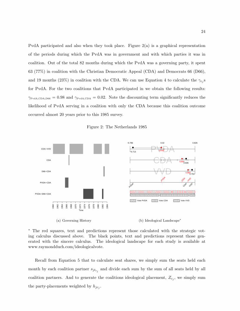
PvdA participated and also when they took place. Figure 2(a) is a graphical representation
of the periods during which the PvdA was in government and with which parties it was in
coalition. Out of the total 82 months during which the PvdA was a governing party, it spent
63 (77%) in coalition with the Christian Democratic Appeal (CDA) and Democrats 66 (D66),
and 19 months (23%) in coalition with the CDA. We can use Equation 4 to calculate the γcj s
for PvdA. For the two coalitions that PvdA participated in we obtain the following results:
γPvdA,CDA,D66 = 0.98 and γPvdA,CDA = 0.02. Note the discounting term significantly reduces the
likelihood of PvdA serving in a coalition with only the CDA because this coalition outcome
occurred almost 20 years prior to this 1985 survey.
Figure 2: The Netherlands 1985
Time
PVDA−D66−CDA
PVDA−CDA
D66−CDA
CDA
CDA−VVD
1960
1962
1964
1966
1968
1970
1972
1974
1976
1978
1980
1982
1984
(a) Governing History
PVDA●
−0.713−0.007
CDA ●
0.6060.504
VVD ●
0.7530.654
PVDACDA
VVD
PVDA
CDAVVD
Vote PVDA Vote CDA Vote VVD
−0.786 0.02 0.826
(b) Ideological Landscape∗
∗ The red squares, text and predictions represent those calculated with the strategic vot-ing calculus discussed above. The black points, text and predictions represent those gen-erated with the sincere calculus. The ideological landscape for each study is available atwww.raymondduch.com/ideologicalvote.
Recall from Equation 5 that to calculate seat shares, we simply sum the seats held each
month by each coalition partner sjtcjand divide each sum by the sum of all seats held by all
coalition partners. And to generate the coalitions ideological placement, Zcj , we simply sum
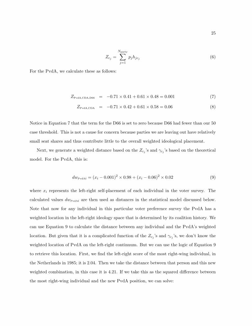
where xi represents the left-right self-placement of each individual in the voter survey. The
calculated values dwPvdAi are then used as distances in the statistical model discussed below.
Note that now for any individual in this particular voter preference survey the PvdA has a
weighted location in the left-right ideology space that is determined by its coalition history. We
can use Equation 9 to calculate the distance between any individual and the PvdA’s weighted
location. But given that it is a complicated function of the Zcj ’s and γcj ’s, we don’t know the
weighted location of PvdA on the left-right continuum. But we can use the logic of Equation 9
to retrieve this location. First, we find the left-right score of the most right-wing individual, in
the Netherlands in 1985; it is 2.04. Then we take the distance between that person and this new
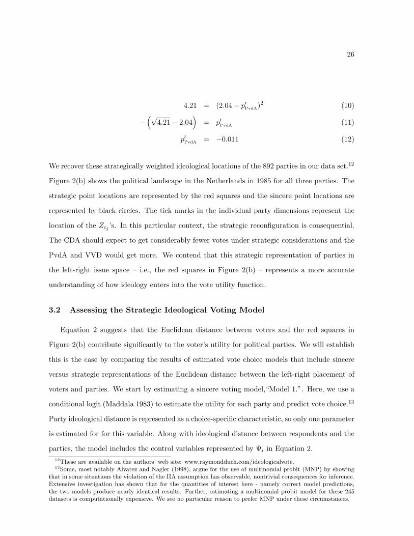
weighted combination, in this case it is 4.21. If we take this as the squared difference between
the most right-wing individual and the new PvdA position, we can solve:
26
4.21 = (2.04− p′PvdA)2 (10)
−(√
4.21− 2.04)
= p′PvdA (11)
p′PvdA = −0.011 (12)
We recover these strategically weighted ideological locations of the 892 parties in our data set.12
Figure 2(b) shows the political landscape in the Netherlands in 1985 for all three parties. The
strategic point locations are represented by the red squares and the sincere point locations are
represented by black circles. The tick marks in the individual party dimensions represent the
location of the Zcj ’s. In this particular context, the strategic reconfiguration is consequential.
The CDA should expect to get considerably fewer votes under strategic considerations and the
PvdA and VVD would get more. We contend that this strategic representation of parties in
the left-right issue space – i.e., the red squares in Figure 2(b) – represents a more accurate
understanding of how ideology enters into the vote utility function.
3.2 Assessing the Strategic Ideological Voting Model
Equation 2 suggests that the Euclidean distance between voters and the red squares in
Figure 2(b) contribute significantly to the voter’s utility for political parties. We will establish
this is the case by comparing the results of estimated vote choice models that include sincere
versus strategic representations of the Euclidean distance between the left-right placement of
voters and parties. We start by estimating a sincere voting model,“Model 1.”. Here, we use a
conditional logit (Maddala 1983) to estimate the utility for each party and predict vote choice.13
Party ideological distance is represented as a choice-specific characteristic, so only one parameter
is estimated for for this variable. Along with ideological distance between respondents and the
parties, the model includes the control variables represented by Ψi in Equation 2.12These are available on the authors’ web site: www.raymondduch.com/ideologicalvote.13Some, most notably Alvarez and Nagler (1998), argue for the use of multinomial probit (MNP) by showing
that in some situations the violation of the IIA assumption has observable, nontrivial consequences for inference.Extensive investigation has shown that for the quantities of interest here - namely correct model predictions,the two models produce nearly identical results. Further, estimating a multinomial probit model for these 245datasets is computationally expensive. We see no particular reason to prefer MNP under these circumstances.
27
Our goal here is to contrast a model incorporating strategic ideological reasoning to that of
Model 1 which assumes sincere ideological reasoning. This is done in two steps. Recall from
Equation 2 and Figure 2(b) that parties can experience two distinct types of movements in
the ideological space as a result of strategic reasoning. First, they can simply drop out of the
strategic voter’s utility calculation. If all of the γcj terms for a particular party are zero then
the strategic component of Equation 2 falls out and there is no strategic voting for that party.
Our theoretical prediction is that voters who are proximate ideologically to these parties should
nevertheless vote for parties that are ideologically more distant but that are in contention to
participate in a governing coalition.
Our second model, “Model 2”, isolates this particular aspect of the strategic ideological
voter’s calculation. To do this we estimate Model 2 that includes only those parties that
have had government experience in the past (i.e., have some element of the vector γcj that is
non-zero). This systematically eliminates some parties from the analysis. In essence we are
comparing the results here to the null model (Model 1) where every individual’s vote is cast
based on Euclidian distance (and the other factors in the model). So, if individuals who were
wrongly predicted in Model 1 to vote for the “non-viable” parties that were closer to them and
are rightly predicted in Model 2 to vote for a viable party that is further away, this is evidence
in favor of our theory. We estimate exactly the same sincere ideological model as Model 1, but
exclude parties that are unlikely to govern.
Our next estimation step is to replace the sincere Euclidean distance term, identified in
Equation 2, with the weighted term. In this model, “Model 3”, both strategic components are
in play: strategic voters are predicted not to vote for parties that have no chance of entering
government (i.e., the vector γcj is all zeros) and ideological distance enters the vote calculus
weighted by the likely coalition participation of parties.
The difference between Model 1 and Model 2 represents the gain in predictive power for
particular parties by simply removing from consideration the parties that are unlikely to be
in government. The difference between Model 2 and Model 3 is the gain in predictive power
for parties by placing the parties at locations that reflects their contribution to coalition policy
outcomes. The theory suggests that there will be significant differences between Models 1 and
28
2 as well as between Models 2 and 3.
4 Results: The Extent of Strategic Ideological Voting
Our theory suggests that ideology is universally important in shaping vote choice; there
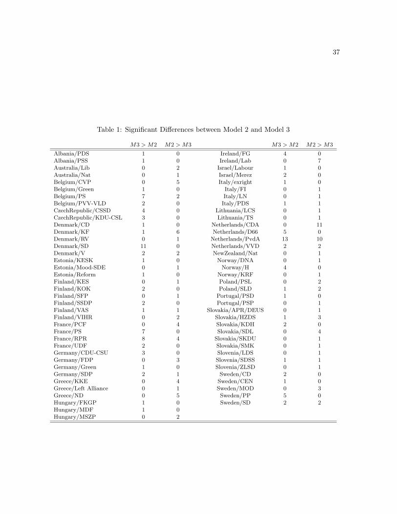
will be contextual variation in the importance of ideology in the vote calculus; and a model
of strategic ideological voting is a better representation of how ideology enters the vote utility
function, i.e., β is large.
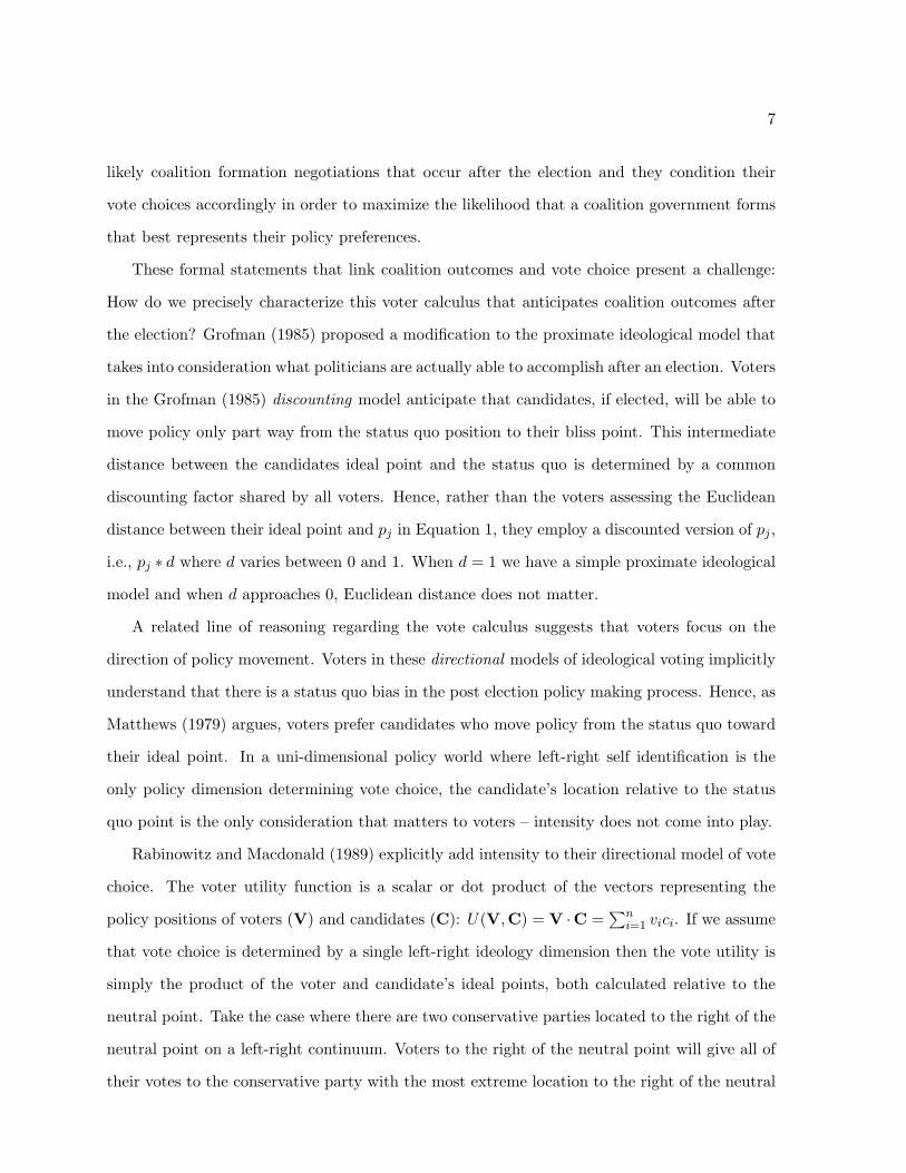
We begin by presenting empirical results that address our first contention, that the ideolog-
ical vote is universal. Here we rely entirely on the Model 1 sincere ideological vote specification.
Recall that we estimate fully specified conditional logit vote choice models for 400 voter prefer-
ence surveys conducted in 57 countries. Hence we have 400 parameter estimates for the sincere
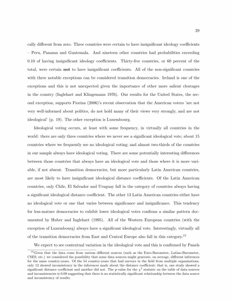
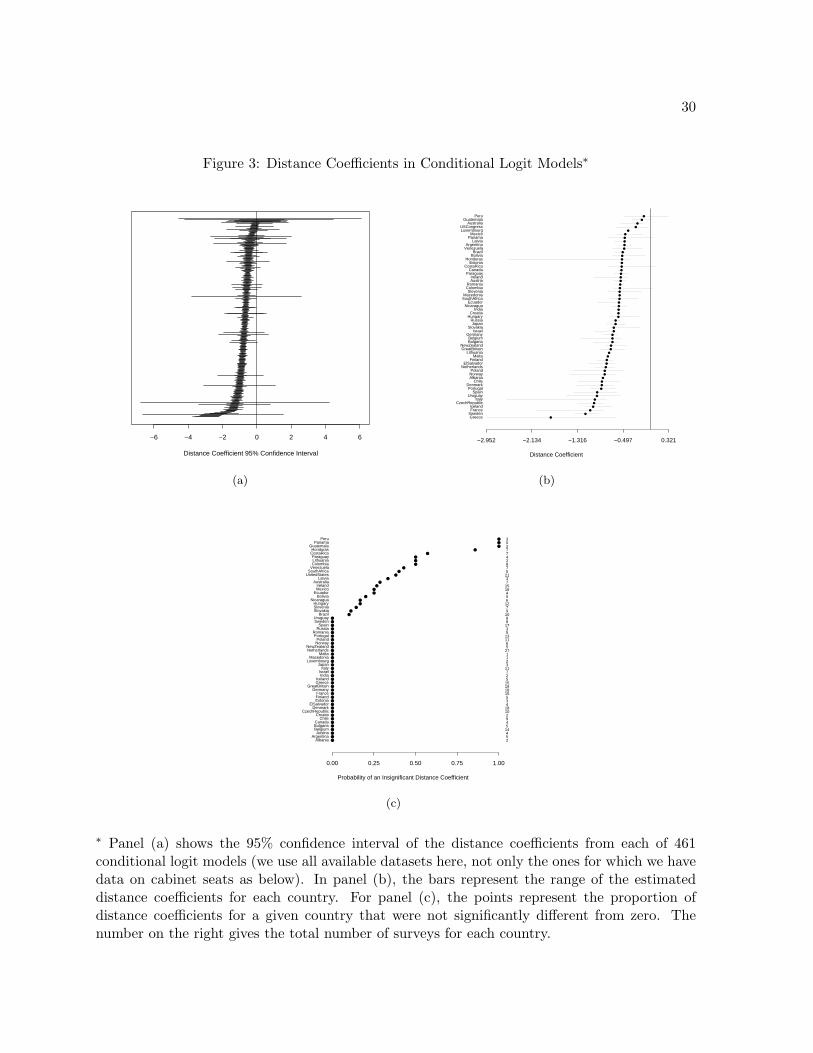
ideological distance term.14 Figure 3(a) shows a dot-plot of these coefficients with a 95% confi-
dence interval imposed and with the lowest coefficient magnitudes at the top of the figure and
highest at the bottom. Most countries have votes that are cast on ideological grounds. Note
that the precision and statistical significance of coefficients varies quite considerably. Recall
that for any country we will have multiple estimates of the ideology coefficient because we have
on average four studies per country, although the average for the more developed democracies
is actually closer to seven (you can see the number of studies associated with each country
in Panel (c)). Panel (b) shows the range of the estimated coefficients for each country - the
minimum and maximum coefficients estimated in the conditional logit models in each coun-
try. The modal distance coefficient is approximately -0.5 and in fact the country distribution
of modal coefficient values is actually quite skewed with most countries clustering around this
value; only a handful of countries exceed this -0.5 value (i.e., have weaker ideological voting);
but a reasonably large number of countries registering quite high ideological voting with modal
coefficient values less than -1.0.
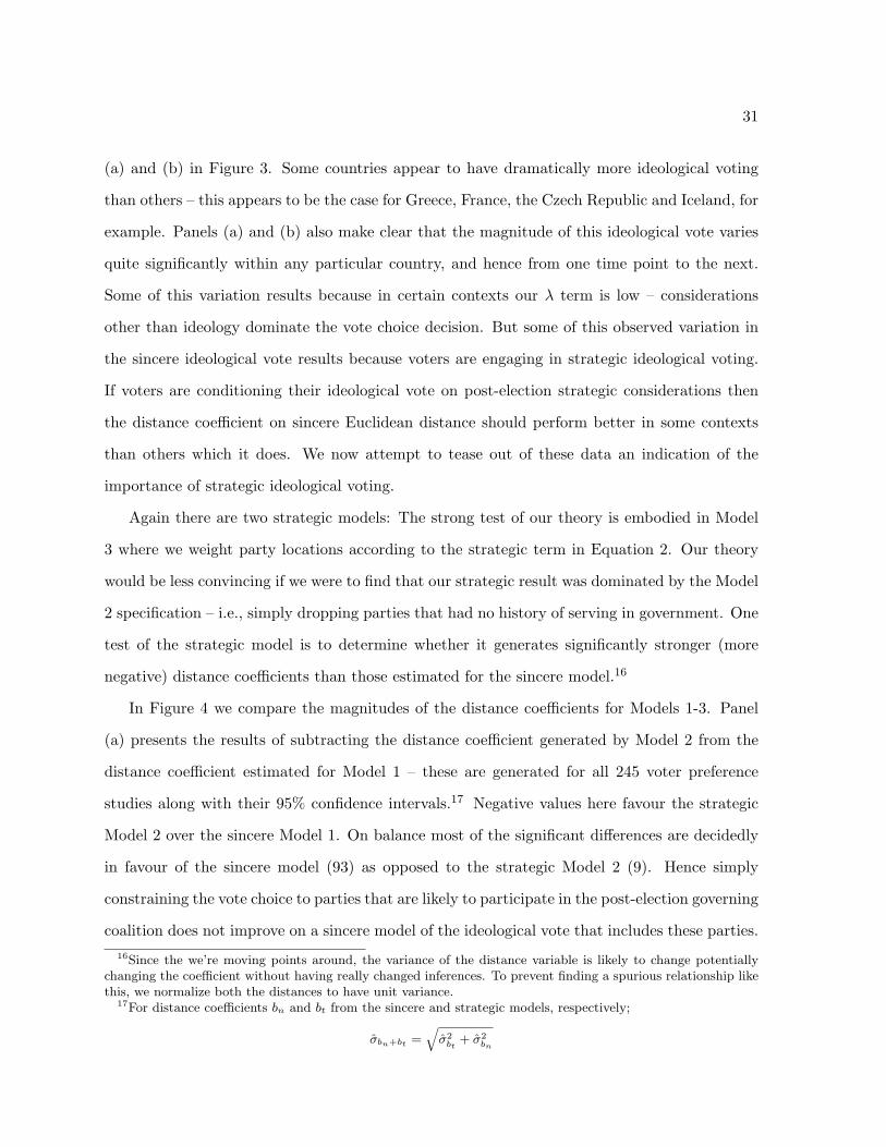
Finally, panel (c) shows the proportion of coefficients in each country that are not statisti-14There are only 245 of these 400 surveys for which we have data on coalition portfolios, thus for Models 2
and 3, we only use that subset of the data presented in Figure 3. However, given the large number of data setscompiled, we thought it would be beneficial to present all of the information across all surveys here.
29
cally different from zero. Three countries were certain to have insignificant ideology coefficients
– Peru, Panama and Guatemala. And nineteen other countries had probabilities exceeding
0.10 of having insignificant ideology coefficients. Thirty-five countries, or 60 percent of the
total, were certain not to have insignificant coefficients. All of the non-significant countries
with three notable exceptions can be considered transition democracies. Ireland is one of the
exceptions and this is not unexpected given the importance of other more salient cleavages
in the country (Inglehart and Klingemann 1976). Our results for the United States, the sec-
ond exception, supports Fiorina (2006)’s recent observation that the American voters ’are not
very well-informed about politics, do not hold many of their views very strongly, and are not
ideological’ (p. 19). The other exception is Luxembourg.
Ideological voting occurs, at least with some frequency, in virtually all countries in the
world: there are only three countries where we never see a significant ideological vote; about 15
countries where we frequently see no ideological voting; and almost two-thirds of the countries
in our sample always have ideological voting. There are some potentially interesting differences
between those countries that always have an ideological vote and those where it is more vari-
able, if not absent. Transition democracies, but more particularly Latin American countries,
are most likely to have insignificant ideological distance coefficients. Of the Latin American
countries, only Chile, El Salvador and Uruguay fall in the category of countries always having
a significant ideological distance coefficient. The other 13 Latin American countries either have
no ideological vote or one that varies between significance and insignificance. This tendency
for less-mature democracies to exhibit lower ideological votes confirms a similar pattern doc-
umented by Huber and Inglehart (1995). All of the Western European countries (with the
exception of Luxembourg) always have a significant ideological vote. Interestingly, virtually all
of the transition democracies from East and Central Europe also fall in this category.15
We expect to see contextual variation in the ideological vote and this is confirmed by Panels15Given that the data come from various different sources (such as the Euro-Barometer, Latino-Barometer,
CSES, etc.) we considered the possibility that some data sources might generate, on average, different inferencesfor the same country-years. Of the 54 country-years that had surveys in the field from multiple organizations,only 12 showed inconsistency in the inferences made about the distance coefficient; that is, one study showed asignificant distance coefficient and another did not. The p-value for the χ2 statistic on the table of data sourcesand inconsistencies is 0.09 suggesting that there is no statistically significant relationship between the data sourceand inconsistency of results.
30
Figure 3: Distance Coefficients in Conditional Logit Models∗
∗ Panel (a) shows the 95% confidence interval of the distance coefficients from each of 461conditional logit models (we use all available datasets here, not only the ones for which we havedata on cabinet seats as below). In panel (b), the bars represent the range of the estimateddistance coefficients for each country. For panel (c), the points represent the proportion ofdistance coefficients for a given country that were not significantly different from zero. Thenumber on the right gives the total number of surveys for each country.
31
(a) and (b) in Figure 3. Some countries appear to have dramatically more ideological voting
than others – this appears to be the case for Greece, France, the Czech Republic and Iceland, for
example. Panels (a) and (b) also make clear that the magnitude of this ideological vote varies
quite significantly within any particular country, and hence from one time point to the next.
Some of this variation results because in certain contexts our λ term is low – considerations
other than ideology dominate the vote choice decision. But some of this observed variation in
the sincere ideological vote results because voters are engaging in strategic ideological voting.
If voters are conditioning their ideological vote on post-election strategic considerations then
the distance coefficient on sincere Euclidean distance should perform better in some contexts
than others which it does. We now attempt to tease out of these data an indication of the
importance of strategic ideological voting.
Again there are two strategic models: The strong test of our theory is embodied in Model
3 where we weight party locations according to the strategic term in Equation 2. Our theory
would be less convincing if we were to find that our strategic result was dominated by the Model
2 specification – i.e., simply dropping parties that had no history of serving in government. One
test of the strategic model is to determine whether it generates significantly stronger (more
negative) distance coefficients than those estimated for the sincere model.16
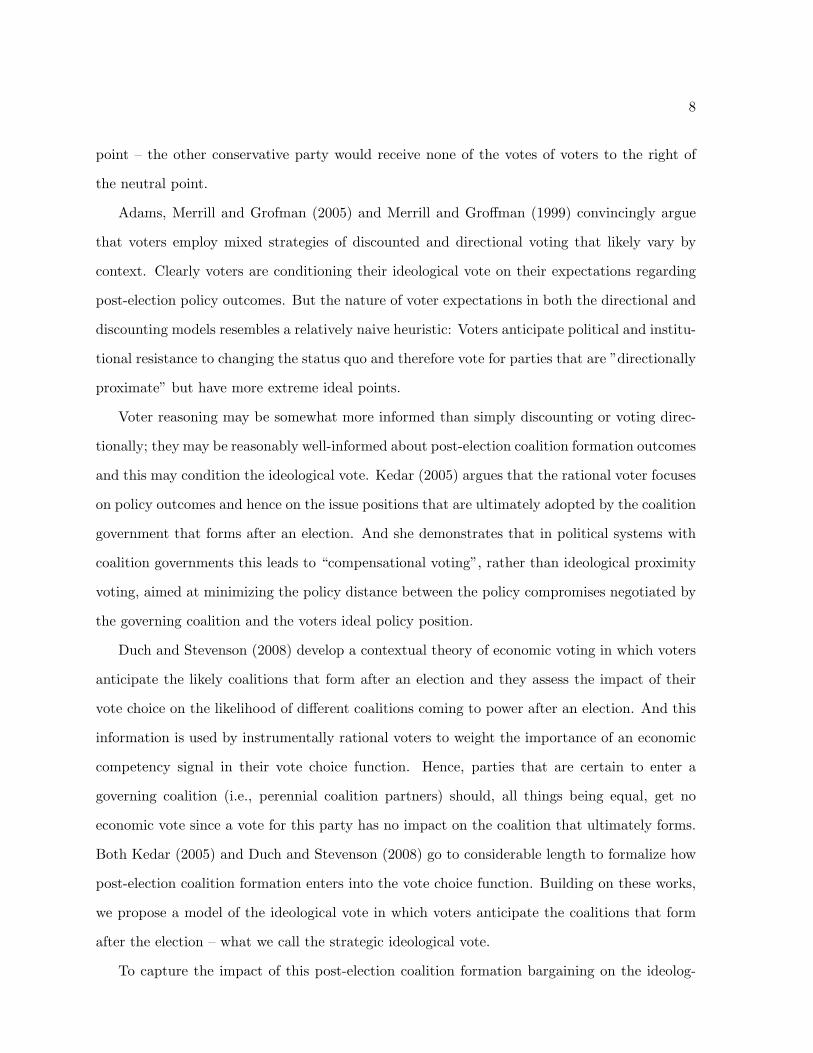
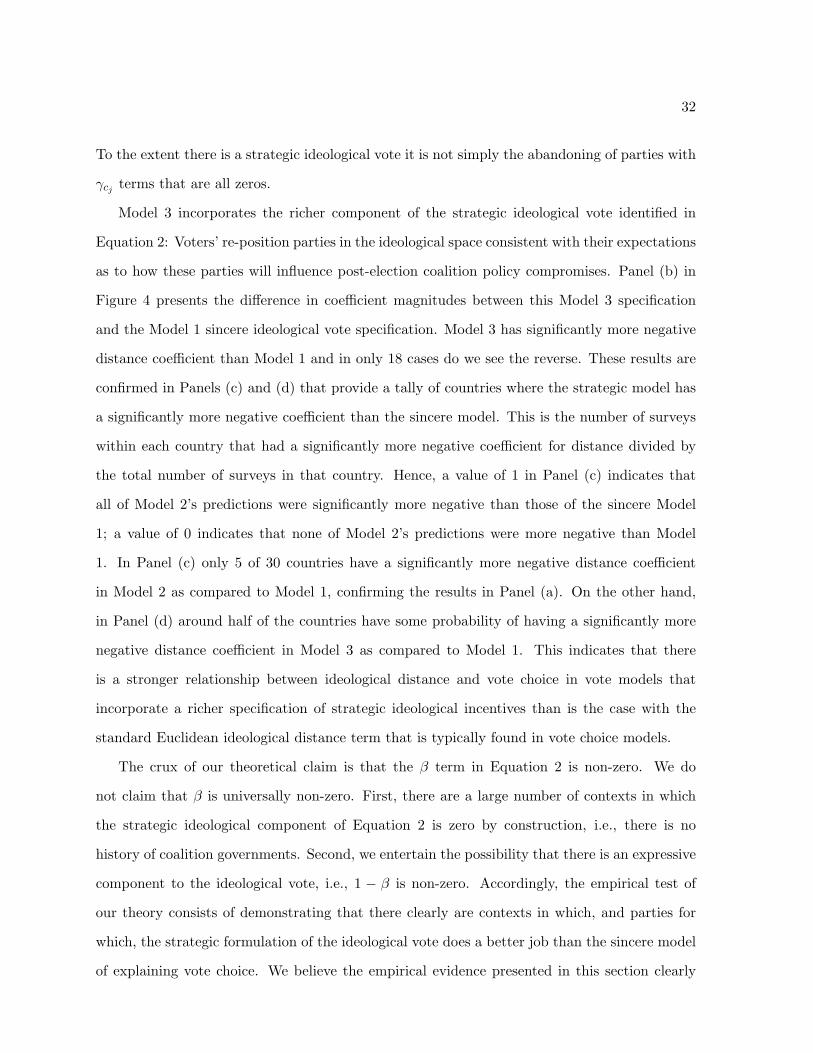
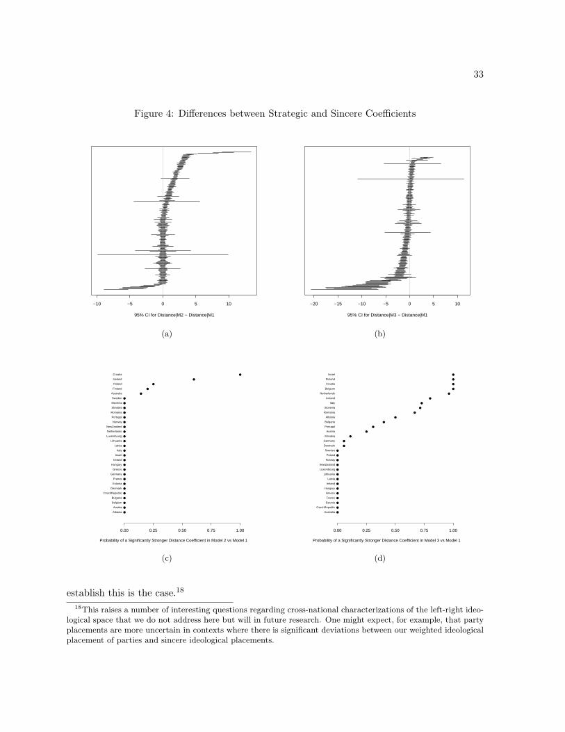
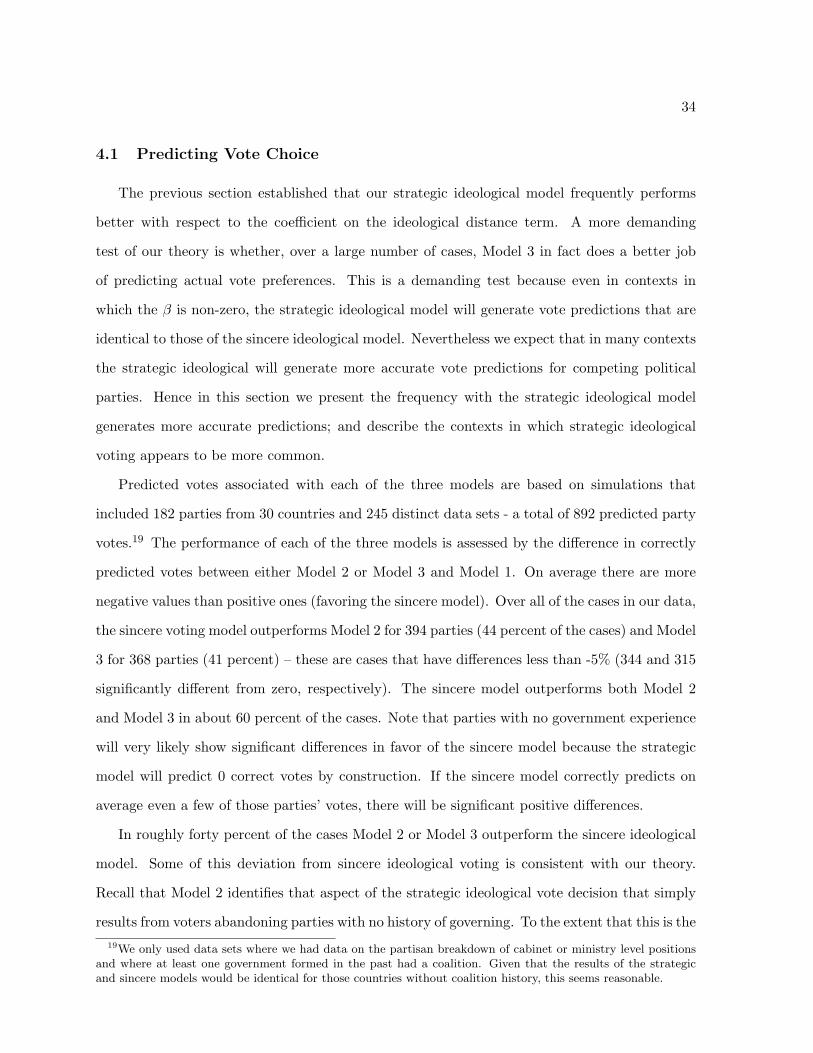
In Figure 4 we compare the magnitudes of the distance coefficients for Models 1-3. Panel
(a) presents the results of subtracting the distance coefficient generated by Model 2 from the
distance coefficient estimated for Model 1 – these are generated for all 245 voter preference
studies along with their 95% confidence intervals.17 Negative values here favour the strategic
Model 2 over the sincere Model 1. On balance most of the significant differences are decidedly
in favour of the sincere model (93) as opposed to the strategic Model 2 (9). Hence simply
constraining the vote choice to parties that are likely to participate in the post-election governing
coalition does not improve on a sincere model of the ideological vote that includes these parties.16Since the we’re moving points around, the variance of the distance variable is likely to change potentially
changing the coefficient without having really changed inferences. To prevent finding a spurious relationship likethis, we normalize both the distances to have unit variance.
17For distance coefficients bn and bt from the sincere and strategic models, respectively;
σbn+bt =√σ2
bt+ σ2
bn
32
To the extent there is a strategic ideological vote it is not simply the abandoning of parties with
γcj terms that are all zeros.
Model 3 incorporates the richer component of the strategic ideological vote identified in
Equation 2: Voters’ re-position parties in the ideological space consistent with their expectations
as to how these parties will influence post-election coalition policy compromises. Panel (b) in
Figure 4 presents the difference in coefficient magnitudes between this Model 3 specification
and the Model 1 sincere ideological vote specification. Model 3 has significantly more negative
distance coefficient than Model 1 and in only 18 cases do we see the reverse. These results are
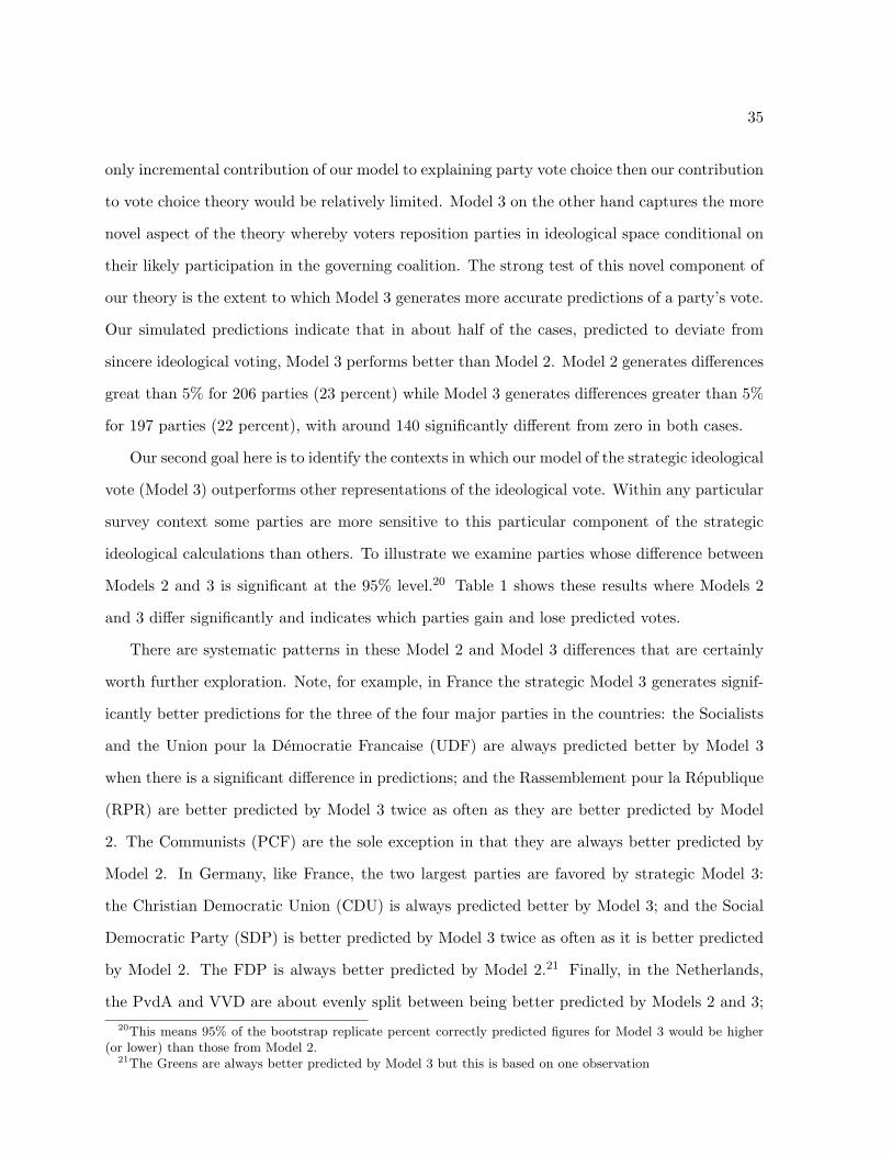
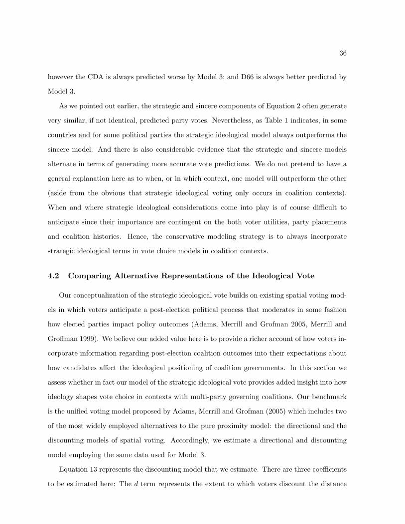
confirmed in Panels (c) and (d) that provide a tally of countries where the strategic model has
a significantly more negative coefficient than the sincere model. This is the number of surveys
within each country that had a significantly more negative coefficient for distance divided by
the total number of surveys in that country. Hence, a value of 1 in Panel (c) indicates that
all of Model 2’s predictions were significantly more negative than those of the sincere Model
1; a value of 0 indicates that none of Model 2’s predictions were more negative than Model
1. In Panel (c) only 5 of 30 countries have a significantly more negative distance coefficient
in Model 2 as compared to Model 1, confirming the results in Panel (a). On the other hand,
in Panel (d) around half of the countries have some probability of having a significantly more
negative distance coefficient in Model 3 as compared to Model 1. This indicates that there
is a stronger relationship between ideological distance and vote choice in vote models that
incorporate a richer specification of strategic ideological incentives than is the case with the
standard Euclidean ideological distance term that is typically found in vote choice models.
The crux of our theoretical claim is that the β term in Equation 2 is non-zero. We do
not claim that β is universally non-zero. First, there are a large number of contexts in which
the strategic ideological component of Equation 2 is zero by construction, i.e., there is no
history of coalition governments. Second, we entertain the possibility that there is an expressive
component to the ideological vote, i.e., 1 − β is non-zero. Accordingly, the empirical test of
our theory consists of demonstrating that there clearly are contexts in which, and parties for
which, the strategic formulation of the ideological vote does a better job than the sincere model
of explaining vote choice. We believe the empirical evidence presented in this section clearly
33
Figure 4: Differences between Strategic and Sincere Coefficients
95% CI for Distance|M2 − Distance|M1
−10 −5 0 5 10
(a)
95% CI for Distance|M3 − Distance|M1
−20 −15 −10 −5 0 5 10
(b)
Probability of a Significantly Stronger Distance Coefficient in Model 2 vs Model 1
●Croatia
●Iceland
●Poland
●Finland
●Australia
●Sweden
●Slovenia
●Slovakia
●Romania
●Portugal
●Norway
●NewZealand
●Netherlands
●Luxembourg
●Lithuania
●Latvia
●Italy
●Israel
●Ireland
●Hungary
●Greece
●Germany
●France
●Estonia
●Denmark
●CzechRepublic
●Bulgaria
●Belgium
●Austria
●Albania
0.00 0.25 0.50 0.75 1.00
(c)
Probability of a Significantly Stronger Distance Coefficient in Model 3 vs Model 1
●Israel
●Finland
●Croatia
●Belgium
●Netherlands
●Iceland
●Italy
●Slovenia
●Romania
●Albania
●Bulgaria
●Portugal
●Austria
●Slovakia
●Germany
●Denmark
●Sweden
●Poland
●Norway
●NewZealand
●Luxembourg
●Lithuania
●Latvia
●Ireland
●Hungary
●Greece
●France
●Estonia
●CzechRepublic
●Australia
0.00 0.25 0.50 0.75 1.00
(d)
establish this is the case.18
18This raises a number of interesting questions regarding cross-national characterizations of the left-right ideo-logical space that we do not address here but will in future research. One might expect, for example, that partyplacements are more uncertain in contexts where there is significant deviations between our weighted ideologicalplacement of parties and sincere ideological placements.
34
4.1 Predicting Vote Choice
The previous section established that our strategic ideological model frequently performs
better with respect to the coefficient on the ideological distance term. A more demanding
test of our theory is whether, over a large number of cases, Model 3 in fact does a better job
of predicting actual vote preferences. This is a demanding test because even in contexts in
which the β is non-zero, the strategic ideological model will generate vote predictions that are
identical to those of the sincere ideological model. Nevertheless we expect that in many contexts
the strategic ideological will generate more accurate vote predictions for competing political
parties. Hence in this section we present the frequency with the strategic ideological model
generates more accurate predictions; and describe the contexts in which strategic ideological
voting appears to be more common.
Predicted votes associated with each of the three models are based on simulations that
included 182 parties from 30 countries and 245 distinct data sets - a total of 892 predicted party
votes.19 The performance of each of the three models is assessed by the difference in correctly
predicted votes between either Model 2 or Model 3 and Model 1. On average there are more
negative values than positive ones (favoring the sincere model). Over all of the cases in our data,
the sincere voting model outperforms Model 2 for 394 parties (44 percent of the cases) and Model
3 for 368 parties (41 percent) – these are cases that have differences less than -5% (344 and 315
significantly different from zero, respectively). The sincere model outperforms both Model 2
and Model 3 in about 60 percent of the cases. Note that parties with no government experience
will very likely show significant differences in favor of the sincere model because the strategic
model will predict 0 correct votes by construction. If the sincere model correctly predicts on
average even a few of those parties’ votes, there will be significant positive differences.
In roughly forty percent of the cases Model 2 or Model 3 outperform the sincere ideological
model. Some of this deviation from sincere ideological voting is consistent with our theory.
Recall that Model 2 identifies that aspect of the strategic ideological vote decision that simply
results from voters abandoning parties with no history of governing. To the extent that this is the19We only used data sets where we had data on the partisan breakdown of cabinet or ministry level positions
and where at least one government formed in the past had a coalition. Given that the results of the strategicand sincere models would be identical for those countries without coalition history, this seems reasonable.
35
only incremental contribution of our model to explaining party vote choice then our contribution
to vote choice theory would be relatively limited. Model 3 on the other hand captures the more
novel aspect of the theory whereby voters reposition parties in ideological space conditional on
their likely participation in the governing coalition. The strong test of this novel component of
our theory is the extent to which Model 3 generates more accurate predictions of a party’s vote.
Our simulated predictions indicate that in about half of the cases, predicted to deviate from
sincere ideological voting, Model 3 performs better than Model 2. Model 2 generates differences
great than 5% for 206 parties (23 percent) while Model 3 generates differences greater than 5%
for 197 parties (22 percent), with around 140 significantly different from zero in both cases.
Our second goal here is to identify the contexts in which our model of the strategic ideological
vote (Model 3) outperforms other representations of the ideological vote. Within any particular
survey context some parties are more sensitive to this particular component of the strategic
ideological calculations than others. To illustrate we examine parties whose difference between
Models 2 and 3 is significant at the 95% level.20 Table 1 shows these results where Models 2
and 3 differ significantly and indicates which parties gain and lose predicted votes.
There are systematic patterns in these Model 2 and Model 3 differences that are certainly
worth further exploration. Note, for example, in France the strategic Model 3 generates signif-
icantly better predictions for the three of the four major parties in the countries: the Socialists
and the Union pour la Democratie Francaise (UDF) are always predicted better by Model 3
when there is a significant difference in predictions; and the Rassemblement pour la Republique
(RPR) are better predicted by Model 3 twice as often as they are better predicted by Model
2. The Communists (PCF) are the sole exception in that they are always better predicted by
Model 2. In Germany, like France, the two largest parties are favored by strategic Model 3:
the Christian Democratic Union (CDU) is always predicted better by Model 3; and the Social
Democratic Party (SDP) is better predicted by Model 3 twice as often as it is better predicted
by Model 2. The FDP is always better predicted by Model 2.21 Finally, in the Netherlands,
the PvdA and VVD are about evenly split between being better predicted by Models 2 and 3;20This means 95% of the bootstrap replicate percent correctly predicted figures for Model 3 would be higher
(or lower) than those from Model 2.21The Greens are always better predicted by Model 3 but this is based on one observation
36
however the CDA is always predicted worse by Model 3; and D66 is always better predicted by
Model 3.
As we pointed out earlier, the strategic and sincere components of Equation 2 often generate
very similar, if not identical, predicted party votes. Nevertheless, as Table 1 indicates, in some
countries and for some political parties the strategic ideological model always outperforms the
sincere model. And there is also considerable evidence that the strategic and sincere models
alternate in terms of generating more accurate vote predictions. We do not pretend to have a
general explanation here as to when, or in which context, one model will outperform the other
(aside from the obvious that strategic ideological voting only occurs in coalition contexts).
When and where strategic ideological considerations come into play is of course difficult to
anticipate since their importance are contingent on the both voter utilities, party placements
and coalition histories. Hence, the conservative modeling strategy is to always incorporate
strategic ideological terms in vote choice models in coalition contexts.
4.2 Comparing Alternative Representations of the Ideological Vote
Our conceptualization of the strategic ideological vote builds on existing spatial voting mod-
els in which voters anticipate a post-election political process that moderates in some fashion
how elected parties impact policy outcomes (Adams, Merrill and Grofman 2005, Merrill and
Groffman 1999). We believe our added value here is to provide a richer account of how voters in-
corporate information regarding post-election coalition outcomes into their expectations about
how candidates affect the ideological positioning of coalition governments. In this section we
assess whether in fact our model of the strategic ideological vote provides added insight into how
ideology shapes vote choice in contexts with multi-party governing coalitions. Our benchmark
is the unified voting model proposed by Adams, Merrill and Grofman (2005) which includes two
of the most widely employed alternatives to the pure proximity model: the directional and the
discounting models of spatial voting. Accordingly, we estimate a directional and discounting
model employing the same data used for Model 3.
Equation 13 represents the discounting model that we estimate. There are three coefficients
to be estimated here: The d term represents the extent to which voters discount the distance
37
Table 1: Significant Differences between Model 2 and Model 3
Following (Adams, Merrill and Grofman 2005) we generate MLE estimates of the λ, α and β
terms in these two unified voter utility models, in addition to the standard proximity model.23
For comparative purposes we employ this same estimation strategy for the λ and β terms in
our Model 3 that was described in Equation 2. From the 245 studies considered, all four utility
models converge in around half (120).24 The results below are from considering these 120
models. Our contention is that the strategic model set forth above is “better” (i.e., provides a
better fit to the data) than the sincere model in at least some circumstances and is not worse22Note that in both models the ideological measure is standardized to have mean zero so that the neutral point
for candidates and voters is zero.23The R code is available on the authors’ web site www.raymondduch.com/ideologicalvote24These results were estimated in R version 2.6.2 using the nlm non-linear maximization routine on computing
resources provided by the Oxford Supercomputing Centre. We used Rmpi version 0.5-5 to distribute the jobs to 16nodes each of which was equipped with 2× dual core Intel Xeon 2.6 GHz (Woodcrest) processors and 4GB DDR2RAM, for a total of 64 processors (of which one was the primary and sixty three were the subordinates). Thetotal run time of the estimation was roughly eight hours (8 × 64 = 512 hours of computing time). Models wereconsidered to have converged if the estimation procedure returned a convergence code of 1 [“relative gradient isclose to zero, current iteration is probably solution”] or 2 [“successive iterates within tolerance, current iterateis probably solution”] and was considered not to have converged if code 3 [“last global step failed to located apoint lower than ‘estimate’. Either ‘estimate’ is an approximate local minimum of the function or ‘steptol’ is toosmall] was returned. The code used in the estimation is available on the authors’ web site.
39
than other strategic representations of a voter’s utility. The data bear out our expectations.
First, we consider the BIC (Bayesian or Schwarz Information Criterion). Since these models
are not technically nested within each other, the BIC is a natural choice for model comparison.
Raftery suggests positive support for a model if it’s BIC is more than two points smaller than
an alternative model (Raftery 1996). First, we look at the cases where the BIC for any one
model is “significantly” better than all of the three other models. These results are in Table 2.
As you can see from the table, there are only 4 studies where our strategic ideological model
dominates all others; and there are 36 studies in which the sincere model is significantly better.
However, there are no instances where either the directional or discounting model dominates
all others. These results suggest, first, that in the vast majority of cases (70 percent) there
is no significant difference amongst the models in terms of model fit. Hence, in most cases
incorporating a richer specification of the voter’s spatial calculus is defensible in terms of model
fit. Secondly, these results indicate that our strategic ideological model is never worse than
the other modified proximity models (discounting and directional) and in fact in a handful of
cases actually generates a better fit statistic. Third, there clearly are cases in which the sincere
ideological model provides a better fit statistic. This, of course, is consistent with our earlier
findings that show variation in the importance of strategic versus sincere ideological voting
across political contexts.25
The next set of results are a little less conservative. Here, we compare the percent of vote
preferences correctly predicted by each model. Table 3 shows the studies in which one model
generates a higher percent of correct predictions than all of the other models (however, these
differences could be, and often are, quite small). Again, there are a number of cases where
our strategic ideological model predicts better than all of its competitors (including the sincere
model). However, there are a number of situations where the sincere model out-predicts all of
the others. As in the previous table, neither the directional nor the discounting models are ever
“better” than all the other models.25Some of the higher fit statistics for the sincere model also may result from the fact that the BIC statistic
tends to favour parsimony in model specification and the sincere model is the most parsimonious of the three.
The point of departure for this essay is the analysis of 400 voter preference surveys, con-
ducted in 57 countries, over a 25 year time period that demonstrates quite definitely that the
41
ideological vote is pervasive in both mature and transition democracies. There is, as we ex-
pected, considerable contextual variation in the ideological vote. Some countries, particularly
transition democracies from Latin America, have quite low levels of ideological voting while in
Western, Eastern and Central Europe it is quite high. The fact that the conventional measures
of ideological voting are both pervasive and variable across contexts is an important necessary
condition for the theory of strategic ideological voting that we develop in this essay.
We argue that rational voters should condition their ideological vote on the likely coalitions
that form after an election since these agreements determine the ideological orientation of gov-
ernment policy. In this essay we develop a model of the ideological vote that incorporates in
the voter’s utility for each party a term consisting of the distance between the voter’s left-right
self-identification and the expected left-right ideological composition of each coalition that a
party might join.
Accordingly, a fully specified empirical model of the vote choice includes a conventional ex-
pressive ideological distance term; our strategic ideological distance term; and controls for the
other factors that typically also affect voting behavior. We assess the independent contribution
of the strategic ideological distance term to the vote decision based on 245 voter preference
surveys from 30 countries. Even though the strategic and sincere ideological terms often gen-
erate predictions that are similar, and frequently exactly the same, we are able to demonstrate
empirically that the strategic ideological distance component of our theoretical model has an
important independent affect on vote choice.
Our representation of the voter’s strategic ideological calculus builds on a body of research,
not dissimilar to ours, that aims to better capture the voter’s anticipation of the ideological
compromises negotiated after an election in contexts with coalition governments. We compare
the explanatory and predictive power of our representation of how voters use ideology in their
vote decision with that of these other models. On balance our strategic ideological model
performs just as well as these other models; for a number of cases it performs better; and
never performs worse. A reasonable conclusion to draw from these results is that our richer
specification of the voter’s strategic ideological vote calculation represents theoretical value
added to our understanding of the vote decision in coalition government contexts.
42
Our specification of the strategic ideological theoretical model, and the empirical results
summarized in this essay, highlight an important feature of, and a challenge associated with,
the study of electoral behavior. There are four terms in our theoretical model of the voter
utility – λ captures the overall importance of ideology; 1− λ indicates the relative importance
of other non-ideological factors in the vote utility function; and 1−β and β indicate the relative
importance, respectively, of sincere versus strategic ideological voting. The relative magnitudes
of these coefficients will vary systematically across countries but also within countries from
one time period to the next. Some countries should never have a strategic ideological vote
and, even for those that typically do, there may be occasions when λ or β are near zero and
hence 1 − λ is uncharacteristically high. If we believe the theoretical model and the empirical
results presented here, then we can only learn about the voter utility function with repetitive
observations from varied political contexts. Hence, as has been pointed out elsewhere (Duch
and Stevenson 2008), we learn very little, and possibly can be seriously mislead, by testing our
theories on a small number of voter preference studies. The challenge presented by these results
is explaining variation in the strategic ideological vote in contexts with multi-party coalition
governments. What contextual factors result in variations in the λ, β, γ terms in our model?
A challenge we hope to take up in future research.
43
References
Adams, James, Benjamin G. Bishin and Jay K. Dow. 2004. “Representation in CongressionalCampaigns: Evidence for Discounting/Directional Voting in U.S. Senate Elections.” Journalof Politics 66:348–73.
Adams, James, Michael Clark, Lawrence Ezrow and Garrett Glasgow. 2004. “UnderstandingChange and Stability in Party Ideologies: Do Parties Respond to Public Opinion or to PastElection Results?” British Journal of Political Science 34:589–610.
Adams, James, Samuel Merrill and Bernard Grofman. 2005. A Unified Theory of Party Com-petition: A Cross-National Analysis Integrating Spatial and Behavioral Factors. Cambridge:Cambridge University Press.
Alesina, Alberto and Howard Rosenthal. 1995. Partisan Politics, Divided Government and theEconomy. Cambridge: Cambridge University Press.
Alvarez, Michael R. and Jonathan Nagler. 1998. “When Politics and Models Collide: EstimatingModels of Multiparty Elections.” American Journal of Political Science 42:55–96.
Austen-Smith, David and Jeffrey Banks. 1988. “Elections, Coalitions and Legislative Out-comes.” American Political Science Review 82:405–22.
Bargsted, Matias and Orit Kedar. 2007. “Voting for Coalitions: Strategic Voting under Pro-portional Representation.” Manuscript.
Blais, A., John H. Aldrich Indridi Indridason and R. Levine. 2006. “Do Voters Vote for Gov-ernment Coalitions?: Testing Downs’ Pessimistic Conclusion.” Party Politics 12:691–705.
Blais, Andre, Donald Blake and Stephen Dion. 1993. “Do Parties Make a Difference?: Partiesand the Size of Government in Liberal Democracies.” American Journal of Political Science37:40–62.
Blais, Andre, Richard Nadeau, Elisabeth Gidengil and Neil Nevitte. 2001. “Measuring StrategicVoting in Multiparty Plurality Elections.” Electoral Studies 20:343–352.
Bowler, Shaun, Todd Donova and Jeffrey A. Karp. 2006. “Strategic Voting Over CoalitionGovernments: The Case of New Zealand.” Unpublished Manuscript.
Budge, Ian and David Robertson. 1987. Do Parties Differ, and How? Comparative Discriminantand Factor Analyses. In Ideology, Strategy and Party Change: Spatial Analyses of Post-WarElection Programmes in 19 Democracies, ed. Ian Budge, David Robertson and Derek Hearl.Cambridge: Cambridge University Press.
Claassen, Ryan L. 2007. “PIdeology and Evaluation in an Experimental Setting: Comparingthe Proximity and the Directional Models.” Political Research Quarterly 60:263–74.
De Sinopoli, Francesco and Giovanna Iannantuoni. 2007. “A Spatial Voting Model whereProportional Rule Leads to Two-Party Equilibria.” International Journal of Game Theory35:267–287.
Downs, Anthony. 1957. An Economic Theory of Democracy. New York: Harper and Row.
44
Duch, Raymond M. and Randy Stevenson. 2008. The Economic Vote: How Political andEconomic Institutions Condition Election Results. Cambridge: Cambridge University Press.
Enelow, James M. and Melvin J. Hinich. 1994. “A Test of the Predictive Diomensions Modelin Spatial Voting Theory.” Public Choice 78:155–69.
Fiorina, Morris. 2006. Culture Wars: The Myth of a Polarized America, 2nd Edition. PearsonLongman.
Grofman, Bernard. 1985. “The Neglected Role of the Status Quo in Models of Issue Voting.”Journal of Politics 47:230–37.
Gschwend, Thomas. 2007. “Ticket-Splitting and Strategic Voting under Mixed Electoral Rules:Evidence from Germany.” European Journal of Political Research 46:1–23.
Huber, John and Ronald Inglehart. 1995. “Expert Interpretations of Party Space and PartyLocations in 42 Societies.” Party Politics 1:73–111.
Indridason, Indridi H. 2007. “Modeling Proportional Representation in Majoritarian Legisla-tures.” Unpublished Manuscript.
Inglehart, Ron and Hans-Dieter Klingemann. 1976. Party Identification and Beyond: Represen-tations of Voting and Party Competition. John Wiley chapter Party Identification, IdeologicalPreference and the Left-Right Dimension among Western Mass Publics.
Irwin, Galen A. and Joop J.M. van Holsteyn. 2003. “They Say it Can’t be Done? StrategicVoting in Multi-Party Proportional Systems: The Case of The Netherlands.” Presented atthe Annual Meeting of the American Political Science Association, Philadelphia, PA.
Kedar, Orit. 2005. “When Moderate Voters Prefer Exterme Parties: Policy Balancing in Par-liamentary Elections.” American Political Science Review 99(2):185–199.
Kedar, Orit. 2006. “Policy Balancing in Presidential Elections: The Effect of PresidentialPowers.” Unpublished Manuscript.
Knutsen, O. 1998. “Expert Judgements of the Left-Right Location of Political Parties: AComparative Longitudinal Study.” West European Politics 21:63–94.
Lacy, Dean and Phillip Paolino. 2005. “Testing Proximity Versus Directional Voting UsingExperiments.” Manuscript.
Laver, Michael and Ian Budge. 1993. “The Policy Basis of Government Coalitions: A Compar-ative Investigation.” British Journal of Political Science 23:499–519.
Macdonald, Stuart Elaine, George Rabinowitz and Ola Listhaug. 2007. “Simulating Models ofIssue Voting.” Political Analysis 15(4):406–427.
Maddala, G.S. 1983. Limited Dependent and Qualitative Variables in Econometrics. Cambridge.
Matthews, Steven A. 1979. “A Simple Direction Model of Electoral Competition.” Public Choice34:141–56.
McCuen, Brian and Rebecca Morton. 2000. “Tactical Coalition Voting.” Working Paper.
45
Meffert, Michael F. and Thomas Gschwend. 2007a. “Polls, Coalition Signals, and StrategicVoting: An Experimental Investigation of Perceptions and Effects.” Unpublished Manuscript(Sonderforschungsbereich 504 No. 07-63).
Meffert, Michael F. and Thomas Gschwend. 2007b. “Strategic Voting under Proportional Rep-resentation and Coalition Governments: A Simulation and Laboratory Experiment.” Unpub-lished Manuscript (Sonderforschungsbereich 504 No. 07-55).
Merrill, Samuel, Bernard Grofman and James Adams. 2001. “Assimilation and Contract Effectsin Voter Projections of Party Locations: Evidence from Norway, France and the U.S.A.”European Journal of Political Research 40:199–221.
Merrill, Samuel III and Bernard Groffman. 1999. A Unified Theory of Voting: Directional andProximity Spatial Models. Cambridge University Press.
Morelli, Massimo. 1999. “Demand Competition and Policy Compromise in Legislative Bargain-ing.” American Political Science Review 93:809–20.
Ortuno-Ortin, Ignacio. 1997. “A Spatial Model of Political Competition and ProportionalRepresentation.” Social Choice and Welfare 14:427–438.
Persson, Torsten and Guido Tabellini. 2000. Political Economics: Explaining Economic Policy.Cambridge: MIT Press.
Poole, Keith T. and Howard Rosenthal. 1997. Congress: A Political-Economic History of Roll-Call Voting. Oxford: Oxford University Press.
Rabinowitz, George and Stuart Macdonald. 1989. “A Directional Theory of Issue Voting.”American Political Science Review 83(1):93–121.
Raftery, Adrian E. 1996. “Approximate Bayes Factors and Accounting for Model Uncertaintyin Generalised Linear Models.” Biometrika 83:251–266.
Rehm, Philipp. 2007. “Political Polarization: Concept Measurement and Result.” Duke Uni-versity.
Snyder, James, Michael Ting and Steven Ansolabehere. 2005. “Legislative Bargaining underWeighted Voting.” American Economic Review 95:981–1004.
Tomz, Michael and Robert P. Van Houweling. 2007. “The Microfoundations of Issue Voting.”Manuscript, August 12, 2007.
Warwick, Paul. 1992. “Ideological Diversity and Government Survival in Western EuropeanParliamentary Democracies.” Comparative Political Studies 25:332–61.
Warwick, Paul. N.d. “Do Policy Horizons Structure the Formation of Parliamentary Gov-ernments: The Evidence from an Expert Survey.” American Journal of Political Science.Forthcoming.
Westholm, Anders. 1997. “Distance Versus Direction: The Illusory Defeat of the ProximityTheory of Electoral Choice.” American Political Science Review 91(4):865085.