1

A Structural Model for Evaluating Preferential Trade Agreements *

Jad Chaaban a , Alban Thomas b†

a University of Toulouse, ESR - INRA b University of Toulouse, LEERNA - INRA

First Version: October 2003 This Version: January 2004

(Please do not quote without permission) Abstract

This paper develops and estimates a structural model of imperfect competition in international markets. The model incorporates a flexible non-linear demand framework with structural price equations, and a general Conjectural Variation approach is developed to characterize strategic interaction. The model is used to evaluate the effects of the signature by a small open economy, Lebanon, of a Preferential Trade Agreement (PTA) with Egypt. Using highly disaggregated trade data and concentrating on the Iron and Steel products, it is shown that the estimated trade creation and/or diversion effects following a PTA are different under the structural approach compared to a reduced form or demand only approach.

Key Words : Preferential Trade Agreements; Imperfect Competition; Structural Econometrics; AIDS demand model. JEL Classification : C51, F13, F14

* The authors would like to thank Basil Fuleihan for his continuous support, Robert Porter for very interesting comments and suggestions, and the staff at the Lebanese Ministry of Economy and Trade for their valuable assistance. The authors are also grateful to the Lebanese Customs Administration, and especially Selim Balaa and Hassan Hneine, for providing the exceptional data set and for their great help and insightful information. The views expressed and remaining errors are solely our own.

† Corresponding Author, University of Toulouse, INRA, 21 Allée de Brienne, Manufacture des Tabacs, Bat. F, 31000, Toulouse, France. Email: thomas@toulouse.inra.fr

2

Introduction

There exists a considerable debate among trade economists with respect to Preferential Trade Agreements (PTAs): on one side there are the proponents of this kind of agreements, who argue that their proliferation will lead eventually, like a domino mechanism, to worldwide free trade in goods and services. Multilateralists, on the other side, argue that these agreements fragment the world trading system, by becoming “stumbling blocks” rather than “building blocks” towards worldwide trade liberalization. Jagdish Bhagwati and Arvind Panagariya, two prominent defenders of multilateral liberalization, argue (Financial Times, 1996) :

While consistent with Article 24 of the General Agreement on Tariffs and Trade, there are now so many Preferential Trade Arrangements (PTAs) such as the North American Free Trade Agreement and the European Union's numerous FTAs with other countries, that a virtual "spaghetti bowl" of crisscrossing preferential trade barriers has arisen, with different duties applying depending on which country the product being imported is assigned to. We are therefore in danger of reproducing the chaos created by the absence of most favored nation status during the 1930s, produced then by protectionism but now, ironically, by free-trade intentions.

Given this, trade diversion appears to be the main concern for the opponents of PTAs. They fear that these agreements will harm the evolution towards global free trade because we run the risk of witnessing a world dominated by a few trading blocks who engage in tariff wars and neo-protectionism against each others. In addition to this, multilateralists raise problematic issues like the rules of origin which harm competition between member and non member countries, and the room for potential trade conflicts created by the presence of overlapping Free Trade Areas. Yet many economists are rather wary of accelerated multilateral liberalization. The argument they raise is that developing countries face the tough challenge of rapid import liberalization and uncertain export earnings, leading to the worsening of their terms of trade in a context where developed economies continue to show tariff and non-tariff barriers in sectors where developing countries have a comparative advantage. As argued in a study of the Third World Network (2001), the quick multilateral liberalization dictated by mainstream trade theory will worsen the economic situation in developing countries because of the presence of several obstacles: 1) Many of the existing agreements are imbalanced against developing countries’ preferences; 2) Developed countries have failed to fulfill their commitments in expanding market access in textile and agriculture and in providing special treatment and assistance; 3) Developing countries face many obstacles in implementing WTO rules; 4) They face intensive pressure to accept new obligations at each round; 5) The decision making process within the WTO is less than transparent or fair and makes developing countries’ participation in decision making rather limited. Some economists go even further. Kaushik Basu states (Project Syndicate, March 2002) :

The perception that the WTO is largely an instrument of the powerful, industrialized nations is broadly correct. To oppose it on all fronts, however, is wrong. A more sophisticated approach towards the WTO (and the North in general) is needed. (...) The WTO says that it is a democratic organization run on the principle of one country, one vote. Anybody who follows the WTO knows that rich countries get around this `nuisance' democratic formality by lobbying behind the scenes to fix the agenda in advance.

This attitude opposing multilateral trade liberalization reflects increased doubt that trade liberalization may not be by itself a growth engine. There is in fact no robust evidence that

3

countries that opened their economy more quickly witnessed increased growth. This adds to the fact that in most instances the causal relationship may not be quite clear: increased growth can also lead to increased trade flows. However, what is commonly admitted is that trade liberalization, when accompanied by sound macroeconomic policy with equitable income redistribution objectives, can lead to better economic development. This cautious attitude towards multilateral trade liberalization can explain why some developing countries have shown a preference to conduct PTAs with their trading partners. These agreements can be negotiated on a case-by-case level, and allow better monitoring and dispute settlements than in broader agreements. In addition to this, small countries feel that they have decision-making power when it comes to bilateral or regional free trade areas, a situation which is far from being achieved within the WTO negotiations. This debate over the right trade liberalization policies has created a vast array of theoretical and empirical studies. While empirically evaluating the welfare impacts of multilateral trade liberalization remains a considerable challenge, the empirical trade literature has focused on evaluating PTAs and the welfare consequences they impose, both on member and non-member countries. The existing studies have been much debated, one major criticism being the fact that they concentrate only on aggregate trade creation or diversion following a PTA, without looking at sector specific effects. Moreover, most of these studies have ignored the role of imperfect competition and strategic interaction in international markets, although these aspects have been extensively treated in the theoretical literature. This paper tries to fill in this gap by developing a structural model of imperfect competition in international markets, using a flexible demand form and a general framework for oligopoly behavior. This model is then used to evaluate the consequences of a PTA signed by Lebanon, a small developing economy, with Egypt. The reason we chose to concentrate on the Lebanese economy is that the Customs Administration there provided us with an exceptional dataset which contains daily trade transactions for a period of 6 years. This dataset contains information on prices and quantities on a very narrow product definition, along with country of origin information, tariffs and application or not of a PTA. The availability of this kind of highly disaggregated trade data makes it possible to evaluate in a relatively precise way the impact of a PTA with respect to trade creation and diversion, within the general structural model we develop. The rest of the paper is organized as follows: Section 1 reviews the theoretical and empirical issues surrounding the analysis of PTAs. In Section 2 the structural model, which forms the core of our analysis, is exposed. We particularly highlight how the demand and supply side specifications interact to form a set of equations that can be easily estimated by employing the Generalized Method of Moments (GMM). Section 3 presents the data used in our empirical estimation. We particularly motivate why the PTA with Egypt has been chosen in our experiment. Section 4 lays down the equations to be estimated, and Section 5 discusses the estimation results and the implications of incorporating a structural analysis into the evaluation of PTAs in general.

1. Economic Analysis of Preferential Trade Agreements

1.1 PTAs: Some definitions

A PTA lowers tariffs among the member countries, while maintaining member protection against non-member trading partners. PTAs contain two kinds of agreements: Free

4

Trade Agreements (FTAs), which allow individual countries to maintain their own tariff against outside countries (like NAFTA), and Customs Unions (CUs), where member countries adopt a common external tariff (like the EU). PTAs are also referred to in the literature as Regional Trade Agreements (RTAs), and are opposed in the trade literature to multilateral broad liberalization agreements (such as WTO accession). During the last 50 years, RTAs increased substantially in number around the world (Figure 1).

FIG. 1. EVOLUTION OF REGIONAL TRADE AGREEMENTS IN THE WORLD, 1948-2002

0

20

40

60

80

100

120

140

160

180

200

1948 1952 1956 1960 1964 1968 1972 1976 1980 1984 1988 1992 1996 2000

Source: WTO Secretariat

As detailed in Anderson (2001), consumers benefit from lower price imports after a PTA, and producers would lower their costs by using cheaper imported inputs. However, producers who compete with these imports might loose due to stiffer competition, and the government looses revenue when tariffs are reduced or eliminated. For this, when free trade increases a country’s welfare, it relates to the gains of this free trade policy exceeding the losses. 1.2 Theoretical assessment of PTAs Bhagwati and Panagariya (1996) present a thorough exposition of the various theoretical currents concerned with PTA analysis. The one we are focusing on, and under which the empirical evaluation of PTAs has been mostly done, is the static analysis. First, under the "Vinerian" approach (named according to Jacob Viner (1950) who pioneered the static analysis of PTAs), free-trade areas (FTAs) and customs unions (CUs) can have positive or negative welfare impacts, both for the member countries and the rest of the world. PTAs could thus be "trade diverting" or "trade creating". A PTA is trade creating for member countries, as demand is increased for partner products, which normally raises their prices, while the opposite occurs for imports from non-partners. Thus, from the point of view of an excluded country, trade diversion in the form of loss of exports to the PTA can be a welfare

Establishment of the WTO

5

deterioration. Moreover, PTA member countries see their trade diverted from low-cost outside suppliers to potentially high-cost within-union suppliers. More recent to the debate is the argument of "natural trading partners", who by forming a PTA will both benefit from trade creation which might outweigh the trade diversion effects; with "natural partners" defined with regards to a high initial volume of trade among them. This argument also relies on the idea that low transport costs between neighbor countries leads to the desirability of PTAs. However, many counter-arguments are presented against this view (see Panagariya (1999) for example). A more optimistic view of custom unions comes from the Kemp-Wan theorem (1976), which shows that it is always possible to form a welfare improving CU among any subset of countries, with no reduction in the non-members' welfare. But this however remains a possibility theorem 1. Other theoretical developments, which are reviewed in Panagariya (2000), include political economy models of trade liberalization bargaining and dynamic evolution models towards tariff elimination, based mainly on general equilibrium settings. 1.3 Empirical evaluation of the effects of PTAs 1.3.1 Traditional empirical approaches The empirical assessment of PTAs (Preferential Trade Agreements) has taken two approaches: First, counter-factual analyses, based on partial or general equilibrium models, with model calibration and simulation. Second, ex-post studies of the arrangements to measure the extent of trade creation and/or trade diversion. The typical approach here is to estimate a “gravity” equation which represents bilateral trade flows as a function of incomes and populations of trading partners, distance between them and membership in a common regional arrangement. An extensive overview of these applied methods for trade policy analysis can be found in François and Reinert (1997). An example of the first approach is the study by Hoekman and Konan (1998), where a competitive, constant returns to scale computable general equilibrium model is used to explore the magnitude of the potential gains from deeper integration within a PTA between the EU and Egypt. Given the fact that Egypt already has a duty-free access to the EU for manufactured products, the authors find that the loss in tariff revenues that will be incurred outweighs any trade creation that will result. They also establish that large welfare gains from an EU FTA are conditional upon the elimination of regulatory barriers and red tape. The second type of empirical evaluation of PTAs has been mainly devoted to answer the following questions: - First, do PTAs contribute to increased trade among member countries? Frankel (1997), by estimating several bilateral gravity equations, answered positively this question. More recently, Soloaga and Winters (1998) applied a gravity model to annual non-fuel imports data, using dummy variables to capture the effects of PTAs. These dummies reflected intra-bloc trade as well as, separately, bloc imports and bloc exports. These bloc-related coefficients were statistically tested for changes “before and after” blocs revival/formation. When allowing for gravity and overall trade effects, the authors found no indication that PTAs boosted intra-bloc trade significantly. When testing intra-bloc trade “before and after” years of bloc

1 On a different level, the Cooper-Massell-Johnson-Bhagwati proposition states that a CU can be a policy measure used to minimize the cost of industrialization in developing countries. See Bhagwati and Panagariya (1996) for more details.

6

revamping/creation, the authors found no statistically significant change in the propensity for intra-bloc trade. - Second, do PTAs cause significant trade diversion? Frankel (1997) argues that NAFTA and the EU caused a great amount of trade diversion, but not enough to harm non-members countries. Soloaga and Winters (1998) found that among most PTAs around the world, only the EU and EFTA showed convincing evidence of trade diversion. Using a similar approach, Cernat (2001) estimated a number of regional trade arrangements among developing countries and explored the gross trade creation and diversion effects resulting from RTA formation. The author found evidence in favor of the idea that South-South RTAs, and African RTAs in particular, are not more trade diverting than other RTAs. - Third, should a closed economy open its trade to all countries or limit itself to participation in regional trade agreements (RTAs)? Vamvakidis (1999) is one of the rare studies to tackle this issue. Based on time-series evidence for a data set for 1950–92, the author estimates and compares the growth performance of countries that liberalized broadly and that of those that joined an RTA. He finds that economies grew faster after broad liberalization, in both the short and the long run, but slower after participation in an RTA. Economies also had higher investment shares after broad liberalization, but lower ones after joining an RTA. All these approaches suffer from serious problems, raised in Panagariya (2000): the first one (computable general equilibrium modeling and calibration) suffers from the fact that it is easy to manipulate the model’s functional forms and parameter values to obtain one’s desired results. The second approach on the other hand has involved mainly the calculation of total quantities of trade creation and trade diversion, and this is insufficient to infer the welfare effects of PTAs. In addition to this, the specification of the distance as an explanatory variable is quite problematic in gravity trade models, as it cannot explain why in many empirical findings distant countries experience intensive trade levels. Panagariya (2000, pp. 326) establishes a necessary solution to these problems:

We need to know trade creation and trade diversion by sector and, in each case, use the information on the decline in the prices of imports to evaluate the benefit from trade creation and the height of trade barriers to measure the damage from trade diversion.

1.3.2 A modern approach: evaluating price effects One recent approach, developed by Winters and Chang (2000), measures the terms of trade effects of regional integration, by looking mainly at the price effects of PTAs. The paper tries to trace the effects of creating a regional trading arrangement on export and import prices. It offers the first ex-post empirical exercise of this kind, by exploring the effects of the Spanish accession to the EU on the prices of imports from major OECD suppliers. Although this paper offers the first evaluation of the change in terms of trade following a PTA, it still suffers from some shortcomings: the reduced form model employed is very simplified and there is no detailed form for import demands. One paper that tries to solve these problems is the paper by Chaaban and Thomas (2003). It offers an approach alongside the above proposition of Panagariya, by giving a framework that allows estimating trade creation and trade diversion by sector, by looking at the changes in import prices and quantities. Chaaban and Thomas (2003) use to this end a flexible demand model, the Almost Ideal Demand System (AIDS), to estimate import elasticities by sector for the Lebanese economy, after identifying imports from major trading blocks. The estimation of a system of flexible import demand equations allows examining the effects of a PTA on each sector’s import quantities and prices, along with an evaluation of sector specific trade creation

7

and trade diversion effects. This study is the first to our knowledge to present such detailed empirical analysis of PTAs, made possible thanks to a highly disaggregated, transaction-based dataset, which was obtained from the Lebanese Customs Administration. The present paper augments the demand system derived and estimated in Chaaban and Thomas (2003) by explicitly modeling the supply-side behavior. The original structural model of oligopoly in international markets allows as we will see below to refine demand side estimates and to evaluate the extent of international competition in sectors that experience trade liberalization.

2. A Structural Model of Imperfect Competition in International Markets

Empirical studies of strategic price behavior in international markets are very few. Goldberg (1995) investigates the effects of trade quotas and the exchange rate pass-through on the U.S. Automobile Industry, by developing a structural model of imperfect competition with product differentiation. Goldberg uses individual data from surveys on the automobile market, enabling her to model demand heterogeneity at a great level of detail. Yet she employs only one competitive equilibrium in her setup, the Bertrand one. Winters and Chang (2000) also use a Bertrand competition setup, but they estimate only a reduced form model with no specific treatment of the demand side. Although their model is the first to explore the effects of regional trade agreements using a setup of imperfect competition in international markets, they estimate terms of trade effects for only two countries at a time (USA vs. EU and Japan vs. EU) exporting to Spain. In a similar spirit, Gil-Pareja (2003) employs a reduced form model with a Bertrand interaction assumption in order to investigate the pricing to market bahaviour in the European car market; showing the existence of international price discrimination in the seemingly homogeneous European market.

The model we develop below offers both a consistent treatment of demand in international markets and allows several competitors to operate on a market at the same time. The model heavily draws from the New Empirical Industrial Organization (NEIO) literature (see Kadiyali et al. (2001) for an excellent overview), where we introduce a structural model of competitive interaction in international markets to empirically test for possible strategic behavior in these markets2. The derived model is a generalization of Dhar et al. (2002), and the model developed below shares with the one in Dhar et al. the following features: First, given that demand specification plays a crucial role in the estimation of market power and strategic behavior, we use a fully flexible “representative consumer model” with a nonlinear Almost Ideal Demand System (AIDS). This avoids the use of approximated or ad-hoc demand specifications that might bias parameter estimates. Second, we use a general Conjectural Variation (CV) approach to model firm behavior, and this allows capturing multi-firm strategic interaction beyond the restrictive Bertrand setting 3. Third, the structural first-order conditions from the firms’ profit maximization program are shown to be solved without the need for linear approximations. They are generic and similar in spirit to the ones in Dhar et al. Because of this, the system of demand and firms’ first order conditions is solved here by employing the Generalized Method of Moments (GMM) estimation technique. Lastly, we provide in our model here an explicit treatment for the expenditure endogeneity problem in

2 For an excellent exposition about the importance and relevance of structural models in econometric analysis see Reiss and Wolak (2002). 3 As shown in Bresnahan (1989) and Kadiyali et al. (2001), the CV approach nests different strategic interaction equilibria (such as Bertrand, collusion, leader-follower, ...), and therefore the estimation of CV parameters allows the researcher to infer and test particular forms of conduct in the setup under consideration.

8

the demand specification, a treatment which is often absent in empirical models of strategic interaction (see Dhar et al. (2002) for more details).

We start by exposing the flexible demand model we intend to use.

2.1 Demand: The Almost Ideal Demand System (AIDS) The most practical way of modeling expenditures with several commodities and various trade regions is to specify a demand system that would satisfy basic economic assumptions on consumer behavior. This demand system should also be simple enough to estimate, and its nature should allow for direct and straightforward inference on consumer reaction to prices. At the same time, an important requisite that has gained much attention in the past decade is that such a demand system be consistent with aggregation. In other words, the final demand for a given good on a market should be obtained by direct aggregation of individual consumer demands. The Almost Ideal Demand System (AIDS) developed by Deaton and Muellbauer (1980) has become one of the most popular demand systems in the economic literature. The purpose of this section is to present a brief exposition of its theoretical foundations. In the economic literature on demand analysis, it is usual to specify a cost or expenditure function for a representative consumer (household or country) as a mathematical expression involving a system of prices for the goods, and the utility (degree of satisfaction) attained when consuming a given set of commodities. For the import demand model, we need to be more explicit on the representation of the price system. Let the subscripts i and j denote distinct imported goods (food, textiles, machinery…), and the subscripts h and k denote sources (regions from which the goods are imported: European Union, North America,…). For each good, the number of sources is not necessarily the same. Let pih denote the unit producer (exporter) price of good i exported from country h. Denoting p the vector (set) of prices and u the utility level of the consumer, the PIGLOG (Price-Independent Generalized Logarithmic) cost function reads

where A(p) and B(p) are parametric expressions of prices:

and

Differentiating the (logarithmic) cost function above with respect to p and u and rearranging, it can be shown that the share of demand for good i from source h, denoted wih, is

where

),p(log)(log)1(),(log BupAupuC +−=

∑∑∑∑∑∑ ++=

i j h kjiji

hi

ikhkhh

ppppA ,loglog*2/1log)(log 0 γα

∏∏+=

i hi

hi

hppApB .)(log)(log 0

ββ

∑∑ ++=

ji

kjkjiihih PEpw

hkh*),/log(log βγα

9

and

Hence, the proportion of imports of good i imported from source j is a function of the price of all other goods from all sources (pjk in the expression above), and also a function of total expenditure divided by an overall price index: E/P*. The price index P* is typically involving all prices from all possible sources, and it can be computed as a weighted price index using as weights the shares in total demand of the goods. Let p0

ih and w0ih respectively denote the base-year (or the empirical mean) of the price and

import share of good i from source h. We can then replace P* by the Tornqvist price index PT whose expression is as follows:

The share equations defined above are valid under very general circumstances for a wide variety of goods. Parameter γihjk for instance captures the sensitivity of the import share of good i from source h with respect to the price of any good j from any source k. Of course, when i=j and h=k, we can measure the reaction of relative demand for a given good to its own price. If we were to use this equation directly, the number of parameters would be tremendous, as it increases both with the number of goods and the number of import sources. A way round this problem is to impose parametric restrictions to the model, by excluding the influence of the price of some goods (or sources) on some other goods (or sources). Imposing restrictions on the AIDS system An interesting reference for restricted AIDS models applied to trade is Andayani and Tilley (1997), who estimate trade diversion elasticities on Indonesian fruit import data. A first restriction concerns source differentiation. Restriction 1. Cross-price effects are not source differentiated between products, but are source differentiated within a product:

For example, the Lebanese demand for European dairy products may have a source-differentiated cross-price effect for dairy products from other sources (North America, Rest of the World), but cross-price responses to non-dairy products are not source-differentiated. This restriction implies an absence of substitutability between products of different nature and different origin. With this restriction, the model is denoted RSDAIDS (Restricted Source Differentiated AIDS) and reads:

)**(2/1hkkhkh ijjiji γγγ +=

∑∑∑∑∑∑ ++=

i j h kjiji

hi

ikhkhh

pppp .loglog*2/1log*log 0 γα

∑∑ +=

i hihihihih

T ppwwP )./log()(2/1log 00

.ijkjiji hkh≠∈∀= γγ

10

where γihk denotes the price coefficients of good i from different source h, and pj is a Tornqvist weighted price index for all goods other than i. We construct this price index as

where p0j and w0

j respectively denote the base-year (or the empirical mean) of the price and the import share of good j over all sources. With Restriction 1, the share of good i imported from source h is seen to depend on prices of the same good from all sources (coefficients γihk), but also on price indexes for all other goods. This may create problems during estimation if the number of goods is prohibitive. Moreover, there are reasons to believe the substitutability patterns between goods may be limited in many cases (for instance, food and machinery, precious stones and chemical products,…). For this reason, we further restrict the model for import shares to be estimated. Restriction 2. Cross-price effects are source differentiated within a product, but are not differentiated across different products. We thus have the final specification for the share equations:

It should be noted that, although price effects for goods other than i in the share equation are not explicitly accounted for, their impact still remains, albeit at a much more aggregated level, through the total expenditure term, log(E/PT). A last set of restrictions does not actually depend on restrictions imposed above on differentiation patterns, but are typically imposed to be consistent with the definition of the expenditure function C defined above. First, coefficients for cross-price effects should be symmetric across equations. For instance, the marginal impact of a change in the price of good i from source h on the share of good i imported from source k should be the same as the marginal impact of a change in the price of good i from source k on the share of good i imported from source h. Restriction 3. Symmetry.

Second, although the latter is specified within the AIDS framework as a flexible functional form, it is immediate that the total expenditure should vary in the same proportion as a uniform change in all prices. For example, if prices for imported goods from all sources increase by 10 percent, we should also have the total expenditure increase by exactly 10 percent. To impose this homogeneity in price for the expenditure function C, we impose parametric restrictions as follows: Restriction 4. Homogeneity in prices.

∑ ∑ +++=

≠k

Tih

ijjjiikiihih PEppw

hhk),/log(loglog βγγα

∑ +=

kjjjjj ppwwp

kk),/log()(log 00

∑ ++=

k

Tihikiihih PEpw

hk)./log(log βγα

.,, khikhhk ii ∀= γγ

11

Inference for demand analysis Once the parametric share equations are estimated, it is possible to infer many substitutability patterns and price effects (see Green and Alston, 1990 for a survey on elasticities in the AIDS model). The most obvious one is given by the so-called Marshallian own-price elasticity, measuring the change in the quantity demanded for good i from source h resulting from a change in its own price: Definition 1. Own-price elasticity of demand.

The second one is the so-called Marshallian cross-price elasticity, measuring the change in the quantity demanded for good i from source h resulting from a change in the price of the same good but from a different source, k: Definition 2. Cross-price elasticity of demand.

The third and last one concerns the expenditure elasticity, i.e., the percent change in total demand for good i when total expenditure on all goods changes: Definition 3. Expenditure elasticity.

The own-price and cross-price elasticities are the central objects of our empirical analysis. With the former, we can predict the change in the quantity demanded for any given commodity from any source, when its price increases or decreases. With the latter, it is possible to assess the degree of trade diversion patterns associated with each good. For instance, an increase in the price of imported European goods relative to North American ones is likely to lead to an increase in imports from North America and a decrease in imports from Europe, but it may also have an impact on goods imported from Arab countries or from the rest of the world. This is because, among other things, additional revenue is obtained because of this decrease in the price of imported goods from Europe, and imports from the rest of the world of competing goods that were not considered for importing may also increase 4. 4 For more information on the centrality of trade elasticities in applied International Trade issues, see Marquez (1990, 1994), who provides an alternative estimation method of bilateral trade elasticities based on time series data.

∑ ∑ ∀=∀=

h kii hiihkh

.,0,1 γα

./1hhhhhh iiiii w βγε −+−=

( ).//1hkhhhkkh iiiiiii www βγε −+−=

./1hhh iii wβη +=

12

2.2 The Supply Side In this section we augment the import demand analysis with a formal treatment of the supply side, by modeling the export behavior of regional partners. In the preceding sections, it was assumed that demand for imports was conditioned on a price system, including customs duties and tariffs, but no attention was paid to strategic price policies by exporters. Here we propose a method that takes this fact into account. The theoretical model proceeds as follows: We assume as in Winters and Chang (2000) that each country is represented by a firm setting its price for exports, while competing with other firms (countries). Each firm from country h produces a good i, and maximizes the following profit function:

Πih = (pih – cih) qih with respect to price, where pih and cih are supply unit price and unit cost respectively, and qih is output quantity. Note that the latter is a function of unit prices from other firms for the same good, and unit prices for other goods. We assume that marginal cost is constant, and that export markets are strategically separable (as in Winters and Chang (2000): there is no attempt by firms to engage in a supergame by considering the interaction between different markets). The first-order condition associated with the firm’s problem is

,0)(,

=

∂

∂

∂

∂+

∂

∂

∂

∂+

∂

∂

∂

∂+

∂

∂−+ ∑ ∑ ∑

≠ ≠ ≠≠hk ij hkij ih

jk

jk

ih

ih

jh

jh

ih

ih

ik

ik

ih

ih

ihihihih p

ppq

pp

pq

pp

pq

pq

cpq

where index j denotes a good different from i, and index k denotes a representative firm from a different country than h. Notice that, in the equation above, price responses to changes in the price of firm h and good i are introduced in three different places. The first term in brackets expresses the reaction of import quantity to its own price (region and commodity category). The second term depends on variations in prices of the same good but from different sources (countries indexed by k). The third term introduces the price reaction for other goods produced within the same country (indexed by j and h), and the fourth term considers the way a change in price pih affects the price of other goods with different sources (indexed by j and k). These terms are denoted Conjectural Variations (CV), and denote firm i conjecture about competitors’ price responses. Let us introduce notation for these three CVs:

.,, ,,,ih

jkihjk

ih

jhihjh

ih

ikihik p

ppp

pp

∂

∂=

∂

∂=

∂

∂= ηηη

As in well known in the economics literature, a CV equal to 1 indicates a cooperative behavior between importers from different regions and for the same commodity. When the Conjectural Variation is strictly positive but different from 1, then the price level of competitors is a significant factor in a representative country’s pricing strategy. The first-order condition above can be written in terms of own and cross-price elasticities. Dividing throughout by total expenditure on product i, and after some manipulations, we have the expression for the optimal pricing policy for good i of a representative firm from region h:

13

,0,,

,,,,,, =

+++×+ ∑∑∑

≠≠≠≠

ihjkjkt

iht

hkijjktihihjh

jht

iht

ijjhtihikih

ikt

iht

hkiktihihtihihtihtiht p

ppp

pp

mww ηεηεηεε

where wiht is the import share of commodity i for region (country) h; miht is the unit mark-up for commodity i in region (country) h; εih,iht is the own-price elasticity of commodity i in region (country) h; εih,ikt is the cross-price elasticity of commodity i between region h and region k; εih,jht is the cross-price elasticity between commodity i and commodity j, for region h. It is not possible to consider the estimation of such an equation with any number of commodities, as the number of parameters increases rapidly with the number of goods and countries. For this reason, it is useful to concentrate on a single commodity group and to consider an aggregate commodity for all other goods. More precisely, we assume that there is no distinct substitution pattern between the commodity of interest and any other good, and that the price of all other goods can be considered having the same role as total expenditure. Furthermore, we impose a restriction on source differentiation: firms make non source-differentiated conjectures between products, in a way that matches the restriction imposed on the demand side:

.,,,, jihihjhjihjkih and ηηγγ == Dividing the price policy equation by wiht x miht, and rearranging, this equation gives the relative price ratio for two firms h and k, and for commodity i:

[ ]

+

++−=

∑

≠≠

−

kkikikih

tik

ihttikihbih

bt

ihtbtihihtih

ihtikihiktih

ikt

iht

pp

pp

mpp

','',

'',,,,

1,,

1ηεηεεηε

where cross-price and income elasticities are written as

,1,1, ,,,

,, −−=+=−= ih

iht

ihihihtih

iht

ihbtih

iht

iktih

iht

ikihiktih www

ww

γγ

εγ

εγγ

ε

and where i is the index of the main commodity, b is the index of the aggregate good, with associated price index pbt. For the latter, this price index is equivalent to the general price index over all commodities, PT. In particular, the cross-price elasticity εih,bt measures the reaction to changes in total import expenditures in the demand for good i. It is interesting to note that, when country k is taken as the reference in the system of demand equations, we obtain a direct way of expressing relative prices (between i and k) as a function of other relative prices and mark-ups. Hence, our structural model provides a simple treatment of price endogeneity (as a decision of the country or firm) in a demand system.

14

3. The Data Data are made available from the Lebanese Customs database, for the years 1997-2002 (6 years). Raw data records consist of daily transactions (both exports and imports) and contain information on:

- day, month and year of the transaction - country of origin (imports) or destination (exports) - preferential or trade agreement tariffs - net quantity of commodity imported/exported (either net weight or number of units) - amount (in Lebanese pounds).

This exceptional dataset allows the close evaluation of the effects of eliminating tariff barriers on a certain commodity group originating from a country that has engaged in a PTA with Lebanon. In fact, Lebanon has signed in recent years several PTAs: one is multilateral, the GAFTA (Greater Arab Free Trade Area), and several others are bilateral with individual Arab countries. Table 1 summarizes import patterns under these PTAs 5. One notices that the share of total imports conducted under these agreements evolved from 3.69% in 1997 to 4.27% in 2002, a share which remains quite low and that is expected to be boosted upward after the Association Agreement with the European Union, Lebanon’s main trading partner, comes into effect in 2007. TABLE 1. IMPORT PATTERNS UNDER PTAs, 1997-2002 Source: Ministry Of Finance - Customs Administration - Customs Information System NAJM- Lebanon Unit: Million USD

Another observation concerning trade agreements is that imports under the multilateral arrangement, GAFTA, remained lower than two major bilateral trade agreements that Lebanon signed with Syria and Egypt respectively. Imports from Syria represented the highest 5 Specific details of these PTAs can be found in Chaaban and Thomas (2003). It is useful to mention that Lebanon is mostly an importing country (imports constitute alomost 85% of its trade balance), and therefore import patterns are largely sensitive to prices affected by PTAs.

1997 1998 1999 2000 2001 2002 Agreements AC 27.2 0.2 56.7 75.1 60.7 59.6 AC GAFTA EG 13.4 0.0 16.2 67.7 67.6 90.8 EG Egypt JO 29.4 29.1 23.8 37.8 17.9 13.7 JO Jordan SA 36.8 43.6 44.2 42.3 13.2 11.1 SA Saudi Arabia SD 13.8 9.2 16.4 14.7 14.3 10.2 SD Sudan SY 154.5 103.9 81.6 73.8 100.2 86.0 SY Syria

KW 0 0 6.2 12.9 3.4 3.5 KW Kuwait IQ 0 0 0 0.4 0.3 0.2 IQ Iraq AE 0 0 0 0 0 4.7 AE Arab Emirates

TOTAL 275.1 186.1 245.1 324.6 277.5 279.8 TOT. IMP. 7456 7060 6206 6228 7291 6445 SHARE % 3.69 2.64 3.95 5.21 3.81 4.34

15

amount among all other bilateral agreements in 1997, yet in 2002 imports from Egypt under the free trade agreement came into the first position. Figure 2 shows how imports from Lebanon’s major free trade partners evolved. Imports from Syria declined sharply between 1997 and 2002, while those from Egypt were on the rise; especially between 2001 and 2002 where global imports were decreasing and Egyptian imports were experiencing the reverse pattern 6. Because of the importance of the agreement with Egypt, it is this PTA that we will concentrate on in this present study. This agreement called for zero tariff rates starting 1-1-1999, with some exceptions applied to agricultural products. It has been crucial in the recent trade liberalization policies carried by Lebanon, and it has proven to be mostly beneficial from Lebanon’s terms of trade perspective, as detailed in Chaaban and Thomas (2003). FIG. 2 : COMPARATIVE IMPORT PATTERNS UNDER PTAs Source : Ministry Of Finance - Customs Administration - Customs Information System NAJM- Lebanon

0

20

40

60

80

100

120

140

160

1997 1998 1999 2000 2001 2002

Mn

USD

AC

EG

JO

SA

SD

SY

TOT IMPx100

TOT IMP: total imports, unit: 100 million USD.

Within this PTA with Egypt, we have chosen to study the Iron and Steel import category. This category of goods is selected because it represents an important import share of Egyptian exports to Lebanon, and because competitors from Europe and America are numerous. The weighted tariff rate applied by the Lebanese Customs on Iron and Steel imports is 8%, and it dropped to 0% on Egyptian Iron and Steel imports after the PTA went into effect in 1999.

6 One reason that could explain this difference between the dynamism of imports under the agreement with Egypt and other agreements like the GAFTA or the one with Syria is that the Egyptian agreement called for immediate zero tariff rates starting 1-1-1999, with some exceptions mainly in agricultural products; while the agreement under GAFTA stipulates a 10% annual reduction starting 1998, and the Syrian agreement imposed that tariff rates on industrial goods would only be reduced by 25% annually starting January 1, 1999; other goods being subject to 50 per cent initial reduction followed by 10 per cent annually over a period of 5 years. The free trade agreement with Egypt thus appears as the most flexible with regards to imports, and this could explain why imports from Egypt grew at a fast rate between 1999 and 2002.

16

This is considered as one of the highest relative decreases in tariffs conceded by Lebanon in recent years. This fact reflects itself in the surge of Egyptian Iron and Steel exports to Lebanon after 1999.

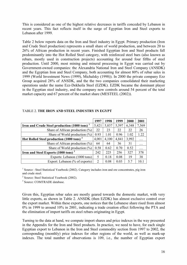
Table 2 below reports data on the Iron and Steel industry in Egypt. Primary production (Iron and Crude Steel production) represents a small share of world production, and between 20 to 26% of African production in recent years. Finished Egyptian Iron and Steel products fall predominantly into the Hot Rolled Steel category, with reinforced steel bars (also known as rebars, mostly used in construction projects) accounting for around four fifths of steel production. Until 2000, most mining and mineral processing in Egypt was carried out by Government-owned companies: the Alexandria National Iron and Steel Company (ANSDK) and the Egyptian Iron and Steel Company, both accounting for almost 80% of rebar sales in 1999 (World Investment News (1999), Michalsky (1998)). In 2000 the private company Ezz Group acquired 28% of ANSDK, and the the two companies consolidated their marketing operations under the name Ezz-Dekheila Steel (EZDK). EZDK became the dominant player in the Egyptian steel industry, and the company now controls around 54 percent of the total market capacity and 67 percent of the market share (MESTEEL (2002)).

TABLE 2. THE IRON AND STEEL INDUSTRY IN EGYPT

Given this, Egyptian rebar sales are mostly geared towards the domestic market, with very little exports, as shown in Table 2. ANSDK (then EZDK) has almost exclusive control over the export market. Within these exports, one notices that the Lebanese share rised from almost 0% in 1999 to around 10% in 2001, indicating a trade creation effect following the PTA and the elimination of import tariffs on steel rebars originating in Egypt.

Turning to the data at hand, we compute import shares and price indexes in the way presented in the Appendix for the Iron and Steel products. In practice, we need to have, for each single Egyptian export to Lebanon in the Iron and Steel commodity section from 1997 to 2002, the corresponding (monthly) price indexes for other regions of the world, as well as mark-up indexes. The total number of observations is 109, i.e., the number of Egyptian export

1997 1998 1999 2000 2001 Iron and Crude Steel production (1000 tons) 1 5,421 5,837 5,597 6,348 7,569

Share of African production (%) 22 23 22 22 26 Share of World production (%) 0.93 1.01 0.96 1.02 1.22

Hot Rolled Steel production (1000 tons) 2 4,001 4,100 4,841 3,992 … Share of African production (%) 64 64 36 31 …

Share of World production (%) 0.58 0.62 0.70 0.52 … Iron and Steel Exports (1000 tons) 3 242 225 256 327 378

Exports: Lebanon (1000 tons) 5 0.18 0.08 19 38 Export: Lebanon (% of exports) 2 0.08 0.03 5.7 10.1

1 Source : Steel Statistical Yearbook (2002). Category includes iron and ore concentrates, pig iron and crude steel. 2 Source: Steel Statistical Yearbook (2002). 3 Source: COMTRADE database.

17

transactions to Lebanon for which we have matching monthly data for other trade partners. These partners are: the European Union (EU), the Arab and Regional countries (AR), North and Latin America (AM) and the Rest Of the World (ROW). On the supply-side, the unit monthly mark-up for Iron and Steel products is computed from the UNIDO 2002 Industrial Statistics Database (4-digit level of ISIC, converted to HS classification), which contains country and sector-wise information on value-added, wage and capital cost, and output value. We assume that the representative exporting firm to Lebanon in each country (or group of countries) applies the same mark-up as the domestic firm in the sector under consideration. This assumption is consistent with the fact that the Lebanese market is quite small and can be regarded as a fringe market with respect to the overall Iron and Steel sales decisions. In addition to this, we compute per unit mark-ups as the ratio of value-added to output, and in the case of country groups we take the average of mark-ups as an indicator for the representative firm’s mark-up. And as this supply-side data is compiled annually, we need to assume that the firm’s monthly mark-up decision only changes from year to year 7. This mark-up measure is not perfect, and the UNIDO database is not comprehensive especially when product specific data is required (at the level of the Iron and Steel industry for example). Yet this database is the only one available where information can be compiled to assess cost differences in manufacturing sectors at a relatively detailed sector level in international markets (4 digit ISIC level). Our present experiment thus shows that it is possible to use this general database without recourse to the almost impossible task of compiling sector-specific product information for all country blocks under consideration. Table 3 below presents descriptive statistics for the sample at hand: TABLE 3. DESCRIPTIVE STATISTICS FOR THE IRON AND STEEL SECTION Variable Mean Standard

Deviation Minimum Maximum

Import Share EU Import share 0.3818 0.1109 0.0377 0.7529 AR Import share 0.0916 0.0671 0.0024 0.4154 AM Import share 0.0825 0.0667 0.0060 0.3752 ROW Import share 0.3041 0.1223 0.0005 0.6291 EG Import share 0.1397 0.0893 0.0080 0.4280

Price Index EU Price index 0.6671 0.1129 0.2915 0.9695 AR Price index 0.8693 0.0973 0.4985 1.0000 AM Price index 0.9148 0.0729 0.6086 0.9926 ROW Price index 0.6980 0.1110 0.4165 0.9984 EG Price index 0.8491 0.1027 0.4761 0.9863

Mark-up EU Mark-up 0.3312 0.0405 0.2878 0.3867 AR Mark-up 0.2557 0.0831 0.1345 0.3805 AM Mark-up 0.5320 0.0081 0.5204 0.5429 ROW Mark-up 0.3485 0.0138 0.3348 0.3768 EG Mark-up 0.2914 0.0059 0.2849 0.3021 Observations : 109. Period: 1997-2002 7 This is not a very crucial assumption, as firms often set their prices and thus their mark-up decisions on a yearly basis, and especially in basic commodity sectors such as the Iron and Steel ones.

18

4. Model Specification and Estimation We estimate a version of the structural model derived above, by considering several competitors to Egypt: European Union (EU), North and South America (AM), Arab and Regional countries (AR), and the Rest of the World (ROW). To reduce the number of parameters to be estimated, we group together Arab and Regional countries with the Rest of the World. The full system of equations to be estimated consists of price policy equations (involving Conjectural Variations terms) and the import demand share equations. For the latter, import price indexes are written in relative form, where price for goods imported from the Rest of the World (ROW) are used as reference. As import prices are considered endogenous here, that is determined by the firm optimal policy on export markets, this must be accounted for to avoid simultaneity bias in estimation. Instruments used are lagged values of import shares for the three different regions, and year dummy variables. Total import expenditure is the corresponding monthly import value for Lebanon. We control for endogeneity of this variable by regressing it on month and year dummies, and price indexes (see also the Appendix for more details). The complete system of equations is written

),/log()/log(

)/log()/log(

,

0T

ttEUEROWtEGtEUEG

ROWtAMtEUAMROWtEUtEUEUEUEUt

PEppppppw

γβ

βββ

++

++=

),/log()/log(

)/log()/log(

,

0T

ttEGEROWtEGtEGEG

ROWtAMtEGAMROWtEUtEUEGEGEGt

PEppppppw

γβ

βββ

++

++=

),/log()/log(

)/log()/log(

,

0T

ttAMEROWtEGtEGAM

ROWtAMtAMAMROWtEUtEUAMAMAMt

PEppppppw

γβ

βββ

++

++=

[ ]

+

+

++

−=

−

EGEUEGt

EUtEGtEUAMEU

AMt

EUtAMtEU

bEUbt

EUtbtEUEUtEU

EUtROWEUROWtEU

ROWt

EUt

pp

pp

pp

mpp

,,,,

,,,1

,,

1

ηεηε

ηεε

ηε

[ ] ,

1

,,,,

,,,1

,,

+

+

++

−=

−

EGAMEGt

AMtEGtAMEUAM

EUt

AMtEUtAM

bAMbt

AMtbtAMAMtAM

AMtROWAMROWtAM

ROWt

AMt

pp

pp

pp

mpp

ηεηε

ηεε

ηε

[ ]

+

+

++

−=

−

EUEGEUt

EGtEUtEGAMEG

AMt

EGtAMtEG

bEGbt

EGtbtEGEGtEG

EGtROWEGROWtEG

ROWt

EGt

pp

pp

pp

mpp

,,,,

,,,1

,,

1

ηεηε

ηεε

ηε

Note that, since the ROW price index is taken as a reference when imposing homogeneity in price to the demand system, we do not estimate cross-price parameters associated with ROW.

19

But from the parametric homogeneity conditions one can replace these coefficients in the last 3 equations by their theoretical counterparts, as functions of other parameters for AM, EG and EU. The full system of equations is estimated by the Generalized Method of Moments (GMM) procedure, using as instruments lagged import price indexes and yearly dummy variables. For a total number of 24 parameters, there are 24 over identifying restrictions, because the total number of orthogonality conditions used to construct the GMM criterion is 48 (8 instruments for each of the 6 equations). The variance-covariance estimation is Newey-West.

5. Results and Discussion

5.1 Structural model estimation results

Estimation results are given in Table 4. As can be seen from this table, parameter estimates for the demand side of the model (coefficients associated to own and cross prices) are significant and have the expected sign, with the exception of the parameter γAM,EG, measuring the reaction of the American import share to the Egyptian price, which is not significantly different from 0. As far as total expenditure is concerned, parameters γE,EG and γE,EU are significantly different from 0, but parameter γE,AM is not, meaning that there is a positive income effect for Egyptian and European imports, but not for American ones. TABLE 4. STRUCTURAL MODEL ESTIMATION RESULTS

Parameter Estimate Std. Error T stat. P-value

β0,AM -0.0506 1.3442 -0.04 0.9700 β0,EG -10.9533 1.7717 -6.18 0.0000 β0,EU -11.7373 3.4780 -3.37 0.0011 γE,AM 0.0149 0.0663 0.23 0.8222 γE,EG 0.5568 0.0878 6.34 0.0000 γE,EU 0.5871 0.1722 3.41 0.0010 γAMAM -0.4876 0.0464 -10.51 0.0000 γAMEG 0.0030 0.0138 0.22 0.8267 γAMEU 0.1792 0.0397 4.51 0.0000 γEGEG -0.6678 0.0963 -6.93 0.0000 γEGEU 0.4667 0.0743 6.28 0.0000 γEUEU -1.1218 0.1728 -6.49 0.0000 ηηηηAM,b -3.96E-7 0.0007 -0.00 0.9996 ηηηηAMEG -18.4019 81.7630 -0.23 0.8224 ηηηηAMEU 0.4031 0.2501 1.61 0.1104 ηηηηAMROW 0.1602 0.0251 6.38 0.0000 ηηηηEG,b -0.00004 0.00005 -0.76 0.4476 ηηηηEGAM 2.0364 8.8889 0.23 0.8193 ηηηηEGEU -0.1067 0.2830 -0.38 0.7070 ηηηηEGROW 0.3683 0.0843 4.37 0.0000 ηηηηEU,b 0.00005 0.0001 0.49 0.6272 ηηηηEUAM -0.0739 0.0473 -1.56 0.1221

20

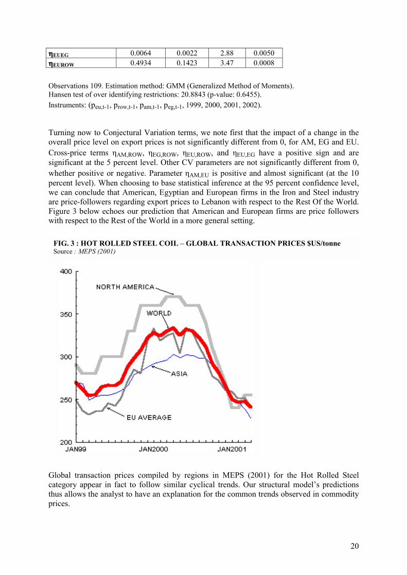
Observations 109. Estimation method: GMM (Generalized Method of Moments). Hansen test of over identifying restrictions: 20.8843 (p-value: 0.6455). Instruments: (peu,t-1, prow,t-1, pam,t-1, peg,t-1, 1999, 2000, 2001, 2002). Turning now to Conjectural Variation terms, we note first that the impact of a change in the overall price level on export prices is not significantly different from 0, for AM, EG and EU. Cross-price terms ηAM,ROW, ηEG,ROW, ηEU,ROW, and ηEU,EG have a positive sign and are significant at the 5 percent level. Other CV parameters are not significantly different from 0, whether positive or negative. Parameter ηAM,EU is positive and almost significant (at the 10 percent level). When choosing to base statistical inference at the 95 percent confidence level, we can conclude that American, Egyptian and European firms in the Iron and Steel industry are price-followers regarding export prices to Lebanon with respect to the Rest Of the World. Figure 3 below echoes our prediction that American and European firms are price followers with respect to the Rest of the World in a more general setting. Global transaction prices compiled by regions in MEPS (2001) for the Hot Rolled Steel category appear in fact to follow similar cyclical trends. Our structural model’s predictions thus allows the analyst to have an explanation for the common trends observed in commodity prices.

ηηηηEUEG 0.0064 0.0022 2.88 0.0050 ηηηηEUROW 0.4934 0.1423 3.47 0.0008

FIG. 3 : HOT ROLLED STEEL COIL – GLOBAL TRANSACTION PRICES $US/tonne Source : MEPS (2001)

21

Furthermore, and this result may seem more surprising, European Iron and Steel exporters take into account Egyptian price variations when designing their own price policies. On the other hand, apart from the prices of Rest of the World countries (including Regional countries), no other regional prices seem to influence the level of Egyptian prices for this category of goods. From the discussion on CV terms above, we can conclude that a collusive (or cooperative) behavior does not exist between Egyptian and European exporters for the Iron and Steel commodities, although the Conjectural Variation exists and is significant. The test statistic for the cooperation assumption (CV=1) between European and Egyptian exporters indicates that this assumption is rejected at the 5 percent level. We have also conducted several other tests on parameter restrictions, in order to evaluate potential strategic interactions. They are summarized in table 5 below, and they were all rejected at the 5 percent level. TABLE 5. CV PARAMETER RESTRICTION TESTS

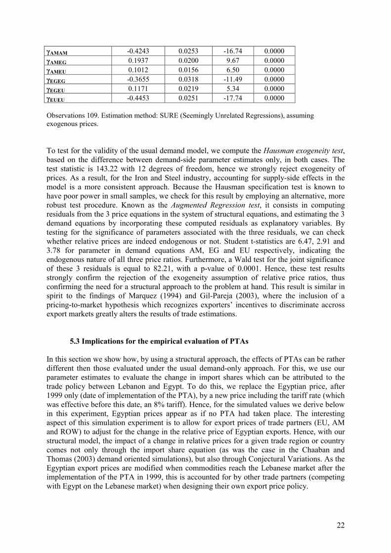
5.2 Testing for the need for a structural approach It is interesting to compare our estimation results for the structural model, in which export prices are assumed endogenous, to estimates obtained under the alternative assumption that the latter are exogenous. In this case, we simply estimate the demand system for the 3 import share equations, that is, dropping the last 3 equations in the system above. As prices are assumed exogenous, the estimation method is Seemingly Unrelated Regressions (SURE). Estimation results are presented in Table 6 below. TABLE 6. USUAL DEMAND MODEL ESTIMATION RESULTS

Parameter Estimate Std. Error T stat. P-value

β0,AM 4.0244 1.6514 2.44 0.0165 β0,EG -0.1585 2.6353 -0.06 0.9522 β0,EU -1.9802 2.6827 -0.74 0.4621 γE,AM -0.1904 0.0815 -2.34 0.0213 γE,EG 0.0160 0.1300 0.12 0.9020 γE,EU 0.1112 0.1324 0.84 0.4027

TEST (restriction) χ2 prob. value Bertrand (ηηηηx,x = 0 for all x)

305.43 0.0000

Bertrand for AM,EG,EU (ηηηηx,x = 0 for all x excl. ηηηηx,ROW) 27.37 0.0001

Symmetry (ηηηηx,y = ηηηηy,x for all x,y excluding ηηηηx,ROW)

13.08 0.0045

Equality (ηηηηx,x for all x) 191.9 0.0000

Equality (ηηηηx,x for all x excl. ηηηηx,ROW) 13.32 0.0206

22

γAMAM -0.4243 0.0253 -16.74 0.0000 γAMEG 0.1937 0.0200 9.67 0.0000 γAMEU 0.1012 0.0156 6.50 0.0000 γEGEG -0.3655 0.0318 -11.49 0.0000 γEGEU 0.1171 0.0219 5.34 0.0000 γEUEU -0.4453 0.0251 -17.74 0.0000 Observations 109. Estimation method: SURE (Seemingly Unrelated Regressions), assuming exogenous prices. To test for the validity of the usual demand model, we compute the Hausman exogeneity test, based on the difference between demand-side parameter estimates only, in both cases. The test statistic is 143.22 with 12 degrees of freedom, hence we strongly reject exogeneity of prices. As a result, for the Iron and Steel industry, accounting for supply-side effects in the model is a more consistent approach. Because the Hausman specification test is known to have poor power in small samples, we check for this result by employing an alternative, more robust test procedure. Known as the Augmented Regression test, it consists in computing residuals from the 3 price equations in the system of structural equations, and estimating the 3 demand equations by incorporating these computed residuals as explanatory variables. By testing for the significance of parameters associated with the three residuals, we can check whether relative prices are indeed endogenous or not. Student t-statistics are 6.47, 2.91 and 3.78 for parameter in demand equations AM, EG and EU respectively, indicating the endogenous nature of all three price ratios. Furthermore, a Wald test for the joint significance of these 3 residuals is equal to 82.21, with a p-value of 0.0001. Hence, these test results strongly confirm the rejection of the exogeneity assumption of relative price ratios, thus confirming the need for a structural approach to the problem at hand. This result is similar in spirit to the findings of Marquez (1994) and Gil-Pareja (2003), where the inclusion of a pricing-to-market hypothesis which recognizes exporters’ incentives to discriminate accross export markets greatly alters the results of trade estimations. 5.3 Implications for the empirical evaluation of PTAs In this section we show how, by using a structural approach, the effects of PTAs can be rather different then those evaluated under the usual demand-only approach. For this, we use our parameter estimates to evaluate the change in import shares which can be attributed to the trade policy between Lebanon and Egypt. To do this, we replace the Egyptian price, after 1999 only (date of implementation of the PTA), by a new price including the tariff rate (which was effective before this date, an 8% tariff). Hence, for the simulated values we derive below in this experiment, Egyptian prices appear as if no PTA had taken place. The interesting aspect of this simulation experiment is to allow for export prices of trade partners (EU, AM and ROW) to adjust for the change in the relative price of Egyptian exports. Hence, with our structural model, the impact of a change in relative prices for a given trade region or country comes not only through the import share equation (as was the case in the Chaaban and Thomas (2003) demand oriented simulations), but also through Conjectural Variations. As the Egyptian export prices are modified when commodities reach the Lebanese market after the implementation of the PTA in 1999, this is accounted for by other trade partners (competing with Egypt on the Lebanese market) when designing their own export price policy.

23

Results are presented in Table 7, where we report the actual and simulated shares, together with the rate of change in import shares for the following trade partners: Egypt, European Union, America (North and South) and the Rest of the World. For the sake of comparison, we also report the same computations based on the usual demand model (AIDS), where prices are assumed exogenous.

TABLE 7. Actual and predicted shares under the No-PTA case, for years 1999 to 2002

Share Actual

Mean, with PTA

Predicted Mean No PTA

Structural model

Predicted Mean No PTA,

Usual demand model

Rate of change (percent)

Structural model

Rate of change (percent)

Usual demand model

wEU 0.3207 0.3725 0.3269 -13.90

-1.89

wROW 0.4651 0.4917 0.4874 -5.41

-4.57

wAM 0.1033 0.0504 0.0994 104.96

3.92

wEG 0.1107 0.0853 0.0861 29.77

28.57

As expected, the Egyptian import share has increased due to the PTA (prices are lower after 1999, and the associated coefficient in the Egyptian share equation is negative), and this increase is rather significant (about 30 percent). Moreover, we also note an increase in the import shares for North and South America, but a decrease for the Rest of the World (recall this trade region includes Arab and Regional countries, excluding Egypt), and the European Union. Although the impact of the PTA with Egypt is rather limited as far as ROW is concerned, the effect is more significant for AM, with an increase of more than 100 percent. This may be explained by the fact that the import share for AM was the lowest, both before and after 1999. Comparing these rates of change with those obtained from the usual demand model one can see that there are major differences for the European Union and especially America. For the latter, the effect of the PTA is predicted as being relatively moderate (an increase of about 4 percent in the import share due to the PTA), whereas it is much more pronounced in our structural model. Hence, overlooking the fact that trade competition may lead regions to adapt their export price policy, depending on the adoption of the PTA by Lebanon, leads to a serious underestimation of the effect of the PTA in the case of AM, and to a large overestimation bias as far as the EU is concerned.

24

Conclusions

This paper has shown how predictions about trade creation and trade diversion following a PTA can be dramatically different when one takes into account the ‘structural framework’ of the problem at hand; that is to include both demand side and supply (export) side effects. By concentrating on a small developing country signing a PTA with another developing country, we were able to show that when a structural model of imperfect competition in international markets is used, predictions about the terms of trade effects on partner and outside countries can be rather different than the ones implied by demand or reduced form models. Moreover, the empirical methodology employed shows that one can combine both national trade statistics with international statistics (such as UNIDO’s) in a way to evaluate on a sector by sector basis the effects of trade agreements on import prices and the import mix in a given country. It would be nice to see our experiment replicated in the context of different countries or regions and for a more aggregated product definition. Combining the COMTRADE and the UNIDO database would probably be interesting to conduct more general PTA evaluation experiments based on our structural model.

Given this, this paper is a first step towards a more comprehensive empirical evaluation of the effects of PTAs. We have only tackled the import side in our experiment, where it was shown that in a particular commodity group the share of imports from a given country or region can increase or decrease following a PTA, and this measures the extent of trade creation or diversion. A general welfare analysis would have to take into account the export side too, where one has to include measures of the PTA-signing country’s exports to partner and non-partner countries. This would allow a general terms of trade assessment, yet would require more data and a more complex setup for modeling import and export behavior simultaneously. This issue remains a major challenge for future research.

25

References Andayani, R.M. and D.S. Tilley (1997). “Demand and competition among supply sources: The Indonesian fruit import market”, Journal of Agricultural and Applied Economics, 29(2), 279-289. Anderson, M. (2001). "Preferential Trade Agreements: Trade Diversion and Other Worries", International Economic Review, USITC publication 3435, p. 5-8, May/June. Basu, K. (2002) “Trade and the Third World”, The Project Syndicate, March. Bhagwati, J. and A. Panagariya. (1996). “The Theory of Preferential Trade Agreements: Historical Evolution and Current Trends”, American Economic Review, Papers and Proceedings, vol. 86 no. 2, p. 82-87, May. Bhagwati, J. and A. Panagariya. (1996). Letter to the Editor, Financial Times, June 25. Bresnahan, T. F., (1989). “Industries with market power”, in The Handbook of Industrial Organization, vol. II, edited by R. Schmalensee and R. D. Willig. Cernat, L. (2001). “Assessing Regional Trade Arrangements: Are South-South RTAs more trade diverting?”, UNCTAD, Study Series n. 16 Chaaban, J. and A. Thomas, (2003). “Assessing the impact of Lebanon’s trade agreements on terms of trade and welfare”, Technical Report, Lebanon Project, UNDP. Dhar, T.P., J.P. Chavas, R.W. Cotterill and B.W. Gould (2002). “An econometric analysis of brand level strategic pricing between Coca Cola and Pepsi Inc.”, University of Wisconsin-Madison working paper. Deaton, A. and J. Muellbauer (1980). “An Almost Ideal Demand System”, American Economic Review, 70, 312-326. François, J.F. and K. A. Reinert, Eds. (1997). Applied Methods for Trade Policy Analysis: A Handbook, Cambridge University Press. Frankel, J.A. (1997). Regional Trading Blocs in the World Economic System. Institute for International Economics. Washington. DC. Gil-Pareja, S. (2003). “Pricing to market behaviour in European car markets”, European Economic Review 47, 945 –962. Goldberg, P. K. (1995) "Product differentiation and oligopoly in international markets: the case of the U.S. automobile industry", Econometrica, vol. 63, no 4, pp 891-951, July. Green, R. and J.M. Alston (1990), “Elasticities in AIDS models”, American Journal of Agricultural Economics, 72, 442-445.

26

Hoekman B. and D. E. Konan. (1998). “Deep Integration, Non-discrimination, and Euro-Mediterranean Free Trade”, presented at the conference Regionalism in Europe: Geometries and Strategies After 2000, Bonn November 6-8. International Iron and Steel Institute (2002). Steel Statistical Yearbook, Committee on Economic Studies, Brussels. Kadiyali, V., K. Sudhir and V.R. Rao (2001). “Structural Analysis of Competitive Behavior: New Empirical Industrial Organization Methods in Marketing”, International Journal of Research in Marketing, 18, 161-186. Kemp, M.C. and H. Y. Wan. (1976). "An Elementary Proposition Concerning the Formation of Customs Unions", Journal of International Economics, vol. 6, p. 95-97. Marquez, J. (1990). “Bilateral trade elasticities”, The Review of Economics and Statistics, vol. 72, pp. 70-77 Marquez, J. (1994). “The econometrics of elasticities or the elasticity of econometrics: An empirical analysis of the behavior of U.S. imports”, The Review of Economics and Statistics, vol. 76, No. 3, pp. 471-481. MESTEEL (2002). Egypt: Steel Industry Overview. Dubai, UAE. MEPS (2001). International Steel Review, April edition. Michalsky, M. (1998). “The mineral industry of Egypt”, U.S. Geological Survey, International Minerals Statistics and Information. Ministry Of Finance, Customs Administration, Customs Information System NAJM. (2002). Trade Data, 1997-2000, Lebanon. Panagariya, A. (1999). Regionalism in Trade Policy : Essays on Preferential Trading, World Scientific Ed. Panagariya, A. (2000). "Preferential Trade Liberalization: The Traditional Theory and New Developments", Journal of Economic Literature, vol. 35, p. 287-331. Reiss, P. and F. Wolak. (2002). “Structural Econometric Modeling: Rationales and Examples from Industrial Organization”, working paper, prepared for The Handbook of Econometrics. Soloaga, I. and A. Winters. (1998). “Regionalism in the Nineties: What Effect on Trade?”, CEPR Discussion Paper Series no. 2183, London: Center for Economic Policy Research. Third World Network. (2001). The Multilateral Trading System : A Development Perspective. UNDP, December. UNIDO (2002). Industrial Statistics Database, 3-and 4-digit level of ISIC, Revision 2 and 3, Vienna.

27

United Nations Statistics Division (2003). Commodity Trade Statistics Database (UN COMTRADE). Vamvakidis, A. (1999). “Regional Trade Agreements or Broad Liberalization: Which Path Leads to Faster Growth?”, IMF Staff Papers, Vol. 46, No. 1 (March) Viner, J. (1950). The Customs Union Issue. New York: Carnegie Endowment for International Peace. Winters, L.A. and W. Chang. (2000). “Regional Integration and Import Prices: an Empirical Investigation”, Journal of International Economics, Vol.51, p. 363-377. World Investment News (1999). Country report : The rebirth of Egypt.

28

Appendix Computation of indices and data handling We construct indicator variables for the region from which the commodity has been exported to Lebanon. The four regions are the following:

- EU (European Union): Andorra, Austria, Belgium, Germany, Denmark, Spain, Finland, France, Great-Britain, Guadeloupe, Gibraltar, Greece, Ireland, Italy, Luxemburg, Martinique, The Netherlands, Portugal, Réunion, Sweden;

- AR (Arab and Regional countries): Algeria, Morocco, Tunisia, Libya, Iraq, Jordan,

Kuwait, Arab Emirates, Bahrain, Brunei, Egypt, Iran, Oman, Qatar, Saudi Arabia, Sudan, Syria, Turkey;

- AM (North and Latin America): United States of America, Canada, Argentina,

Bolivia, Brazil, Bahamas, Chile, Colombia, Costa Rica, Dominican, Ecuador, Guatemala, Honduras, Mexico, Panama, Peru, Paraguay, Trinidad and Tobago, Uruguay, Venezuela;

- ROW (Rest of the World).

These regions are defined in a narrow economic sense in the case of the European Union, and in a more geographic sense for AR (Arab and Regional countries) and AM (North and Latin America). The daily observations on price and quantity are then aggregated by computing monthly equivalents of price and quantity. To do this, we define the HS8 (Harmonized System 8 Digit) level as the base unit for the empirical analysis. This choice is motivated by the need to preserve a reasonable level of homogeneity for commodities. For each good defined as a specific HS8 level, we compute the monthly average of daily unit prices, and the monthly level of imports as the sum of quantities imported over all days of the month. Monthly import shares by region are computed by dividing import value from each region by total expenditure for the same good and the same month. For commodity j imported from source k at time (month) t, we have

.// ttjtji h

tititjtjtj EQpQpQpwkkhhkkk

== ∑∑

Finally, we need to compute regional price indexes in order to capture differences in price levels among export regions (EU, AR, AM and ROW). For each good j (defined at the HS8 level) and month t, we construct an import-share-weighted Tornqvist price index as follows:

where wjkt denotes the share of good j imported from source k (EU, AR, AM or ROW) at time t, pjkt is the price of good j imported from source k; w0

k and p0k are the average (over all time

periods) import share and price for source k, respectively. Individual goods are defined at the HS8 (Harmonized System, 8 Digit) level. But since there are not enough monthly observations for each good to consistently estimate parameters of the RSDAIDS model, we need to further restrict model specification. More precisely, we impose parameters in the share equations to be the same for all goods within each section. The latter

∑ +=

kktjktjjt ppwwp

kk),/log()(log 00

29

represents a broader category of commodities, also denoted HS1 (Digit 1): there are 21 sections for 97 HS2 (chapter) levels, and 5666 HS8 levels. The share equations corresponding to the Restricted Source Differentiated AIDS demand system imply not only price indexes for various import sources as explanatory variables, but also the logarithm of expenditure over the overall price index, log(E/PT). This expenditure is an endogenous variable in the statistical and economic sense, as it depends on the whole price system including region-specific import unit price indexes. For this reason, it is common practice in applied demand analysis to replace discounted expenditure by a prediction computed from instruments such as time dummies and a selection of prices. In a first step, we regress the term log(E/PT) on monthly dummy variables and region-wise price indexes. The linear prediction is then used in place of the original variable in the share equations. With such a procedure, parameter estimates are expected to be consistent. We also include in the share equations a set of yearly dummy variables from year 1998 to year 2002 (the first year, 1997, is dropped from the equation because these dummies would sum to 1). This allows one to control for any trend in demand that might affect regional share levels. Details of the PTA with Egypt (source: Chaaban and Thomas (2003)) The Executive Programme to Enhance Trade Exchange between the Lebanese Republic and the Egyptian Arab Republic within the Framework of the Taysir Agreement was signed on the 10th of September 1998 and ratified on the 23rd of February 1999. This agreement calls for zero duties as of January 1, 1999, with the following exceptions: - Free trade does not apply on 9 groups of goods of Egyptian origin when imported into Lebanon. Such goods are however subject to GAFTA agreement reductions. These are in chapter 6, 16, 24, 769, 84, and 94 8. - Free trade does not apply on 7 groups of goods of Lebanese origin when imported into Egypt. These are in chapters 2, 22, 24, 25, 50, 63, 74, 76, 85, and 87. - For 6 groups of agricultural goods of Egyptian origin, free trade applies during a certain period of the year when such goods are imported into Lebanon. During the remaining period of the year, such products are prohibited from importation into Lebanon. These are in chapters 7 and 8. - For 4 groups of agricultural goods of Lebanese origin, free trade applies during a certain period of the year when such goods are imported into Egypt. During the remaining period of the year, such products are prohibited from importation into Egypt. These are in chapter 8. - Sixteen groups of agricultural goods of Egyptian origin are prohibited from import into Lebanon. These are in chapters 1, 2, 4, 7, 8, 11, 15, and 20. - Ten groups of goods of Lebanese and Egyptian origins are subject to gradual reductions (25 per cent per year) starting 1 January 1999 leading to free trade for these groups of goods within 4 years. These are in chapters 4, 7, 8, 17, 20, 22, and 32. - Five groups of goods of Egyptian origin are subject to prior permit when imported into Lebanon. These are in chapters 25, 74, 76, and 85.

8 Chapter numbers are based on the International Harmonized System (HS) classification.