Page 1
A Structured Approach to Defining Active
Suspension Requirements
Ashwin M Rao
Thesis submitted to the faculty of the Virginia Polytechnic Institute and State University
in partial fulfillment of the requirements for the degree of
Master of Science
In
Mechanical Engineering
Steve Southward (Chair)
Mehdi Ahmadian
Corina Sandu
July 15th, 2016
Blacksburg, VA
Keywords: Active Suspension, Ideal Control Force, Quarter-car, LMS, Road Obstacle
Copyright 2016, Ashwin M Rao
Page 2
A Structured Approach to Defining Active Suspension Requirements
Ashwin M Rao
ABSTRACT
Active suspension technologies are well known for improving ride comfort and handling
of ground vehicles relative to passive suspensions. They are ideally suited for mitigating
single-event road obstacles. The work presented in this thesis aims to develop a structured
approach for finding the peak force and bandwidth requirements of actuators for active
suspensions, to mitigate single-event road obstacles. The approach is kept general to allow
for application to different vehicle models, ride conditions and performance objectives.
The current state-of-art in active suspensions was first evaluated. Based on these findings,
the objectives of the simulation models and approach was defined. A quarter-car model
was developed in Matlab to simulate the behavior of active suspensions over unilateral
boundary conditions due to different road obstacle profiles. The obstacle profiles were
obtained from existing standards and literature and then processed to replicate the
interaction of tires on road. A least-mean-squares (LMS) algorithm for adaptive filtering,
with the help of look-ahead preview was used to determine the ideal control force profile
to achieve the performance objective of the active suspension. A case study was conducted
to determine the requirements of the actuator in terms of bandwidth and peak force for
different single-event road obstacle profiles, vehicle speeds and look-ahead preview
distances. The results of the study show that the vehicle velocity and type of road obstacle
have a strong influence on the required peak force and bandwidth of the actuator, while
look-ahead preview will be much more important for real time controller implementation.
Page 3
iii
Acknowledgements
I would like to thank my academic advisor Dr. Steve Southward for giving me the
opportunity to work on this research and the guidance to complete my thesis. His courses
on Applied Linear Systems and Control were two of my favorite courses at Virginia Tech
and gave me the theoretical and practical foundation to solve the problems I encountered
during my research.
I would also like to thank Dr. Mehdi Ahmadian and Dr. Corina Sandu for their participation
in my thesis committee and taking the time to evaluate my work.
I would like to thank my roommates, friends and all the people of Virginia Tech for making
my time in a place halfway around the globe from my home, both enjoyable and
memorable. I cherish every day in this wonderful university and country.
Most of all, I want to thank my parents for their support and encouragement throughout
my education and graduate studies which allowed me to excel academically and overcome
all the obstacles I encountered in my life.
Page 4
iv
Table of Contents
Acknowledgements .......................................................................................................... iii
Table of Contents ............................................................................................................. iv
List of Figures ................................................................................................................... vi
List of Tables .................................................................................................................. viii
1 Introduction ................................................................................................................1
1.1 Background .......................................................................................................... 1
1.2 Motivation ............................................................................................................ 1
1.3 Objectives ............................................................................................................. 2
1.4 Approach .............................................................................................................. 2
1.5 Outline .................................................................................................................. 3
2 Literature Review .......................................................................................................4
2.1 Active Vehicle Suspensions ................................................................................. 4
2.2 Road Profiles ........................................................................................................ 5
2.3 Adaptive Filtering ................................................................................................ 6
3 System Model ..............................................................................................................7
3.1 Assumptions ......................................................................................................... 7
3.2 Model Description ................................................................................................ 8
4 Unilateral Boundary Conditions .............................................................................14
4.1 Road Obstacles ................................................................................................... 14
4.1.1 Curbs ........................................................................................................... 15
4.1.2 Speed Humps and Speed Bumps ................................................................ 17
4.1.3 Potholes ....................................................................................................... 18
4.1.4 Uneven Road Profile ................................................................................... 20
Page 5
v
4.1.5 Random Road Profile Generation ............................................................... 21
4.2 Pre-processing Road Profiles ............................................................................. 27
4.2.1 Tandem Elliptical Cam Pre-Processing ...................................................... 27
4.2.2 Low-Pass Filtering ...................................................................................... 32
4.2.3 Obtaining Vertical Velocity Profile ............................................................ 33
5 Optimized Control Force Estimation .....................................................................35
5.1 LMS Optimization.............................................................................................. 35
5.1.1 Iterative LMS Adaptation ........................................................................... 38
5.2 FIR Filter Model................................................................................................. 42
5.2.1 Model Regeneration .................................................................................... 44
6 Results ........................................................................................................................46
6.1.1 Case study results: Curb A .......................................................................... 53
6.1.2 Case study results: Pothole P1 .................................................................... 54
6.1.3 Case study results: Speed Hump Watts Profile ........................................... 55
6.1.4 Case study results: Uneven Road A ............................................................ 56
7 Conclusions ...............................................................................................................57
7.1 Contributions ...................................................................................................... 57
7.2 Future Work ....................................................................................................... 58
8 References .................................................................................................................59
9 Appendix ...................................................................................................................61
Page 6
vi
List of Figures
Figure 3.1: Quarter-car model............................................................................................. 8
Figure 3.2: Free body diagram of (a) sprung mass, (b) unsprung mass.............................. 9
Figure 3.3: Inputs and outputs of quarter-car model......................................................... 10
Figure 3.4: Transfer functions of quarter-car model ......................................................... 12
Figure 4.1: Standard curb profiles .................................................................................... 15
Figure 4.2: Standard curb profiles in Matlab .................................................................... 16
Figure 4.3: Speed hump profiles ....................................................................................... 17
Figure 4.4: Speed hump profiles in Matlab ...................................................................... 18
Figure 4.5: Pothole profile ................................................................................................ 19
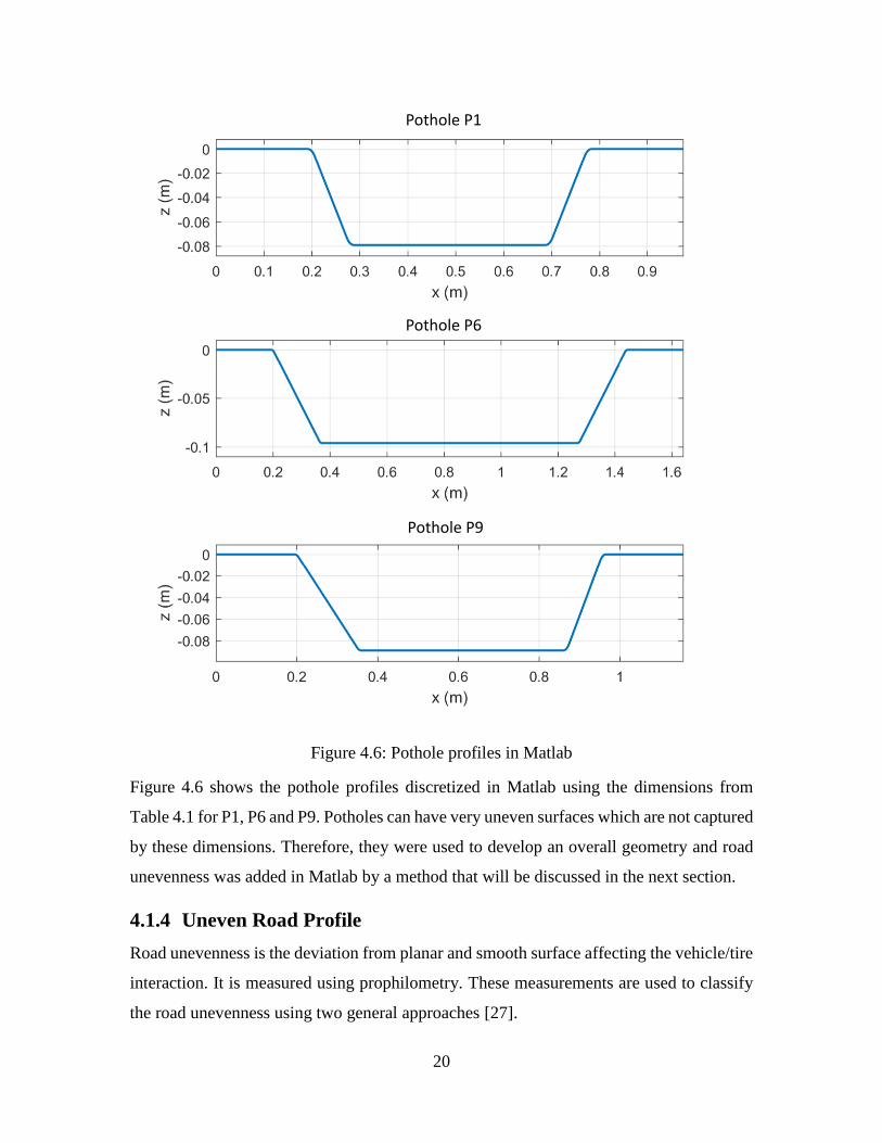
Figure 4.6: Pothole profiles in Matlab .............................................................................. 20
Figure 4.7: ISO 8608 road surface classification .............................................................. 22
Figure 4.8: Random road profiles generated in Matlab .................................................... 25
Figure 4.9: Uneven road profiles ...................................................................................... 26
Figure 4.10: Filtering of road profile ................................................................................ 27
Figure 4.11: Generation of basic curve ............................................................................. 28
Figure 4.12: Tandem Elliptical Cams ............................................................................... 30
Figure 4.13: Filtering of road profile using tandem elliptical cams ................................. 32
Figure 4.14: Processing of road profiles ........................................................................... 33
Figure 4.15: Unilateral boundary condition ...................................................................... 34
Figure 5.1: Adaptive linear combiner ............................................................................... 36
Figure 5.2: LMS algorithm ............................................................................................... 37
Figure 5.3: Filtered-X LMS Algorithm ............................................................................ 37
Figure 5.4: Iterative LMS Adaptation of filter coefficients .............................................. 38
Figure 5.5: Iterative LMS Adaptation – poor performance .............................................. 39
Figure 5.6: Iterative LMS Adaptation - good performance .............................................. 40
Figure 5.7: Fx-LMS algorithm applied to quarter-car model ........................................... 41
Figure 5.8: FIR filters for transfer function paths ............................................................. 43
Figure 5.9: Transfer functions for quarter-car model ....................................................... 44
Figure 5.10: Velocity input comparison ........................................................................... 45
Figure 6.1: Iterative LMS Adaptation applied to quarter-car ........................................... 47
Page 7
vii
Figure 6.2: Controlled quarter-car model response .......................................................... 48
Figure 6.3: 80% Power Bandwidth ................................................................................... 49
Figure 6.4: Peak force surface for non-converged filter W ............................................. 51
Figure 6.5: Peak force surface for converged filter W ..................................................... 52
Figure 6.6: Results for Curb A .......................................................................................... 53
Figure 6.7: Results for Pothole P1 .................................................................................... 54
Figure 6.8: Results for Speed Hump Watts Profile........................................................... 55
Figure 6.9: Results for Uneven Road A ............................................................................ 56
Figure 9.1: Speed Hump Watts Profile ............................................................................. 61
Figure 9.2: Speed Hump Seminole Profile ....................................................................... 61
Figure 9.3: Curb A ............................................................................................................ 62
Figure 9.4: Curb B ............................................................................................................ 62
Figure 9.5: Curb C ............................................................................................................ 63
Figure 9.6: Curb D ............................................................................................................ 63
Figure 9.7: Curb E............................................................................................................. 64
Figure 9.8: Curb F ............................................................................................................. 64
Figure 9.9: Curb G ............................................................................................................ 65
Figure 9.10: Uneven Road A ............................................................................................ 65
Figure 9.11: Uneven Road B ............................................................................................ 66
Figure 9.12: Uneven Road C ............................................................................................ 66
Figure 9.13: Pothole P1..................................................................................................... 67
Figure 9.14: Pothole P6..................................................................................................... 67
Figure 9.15: Pothole P9..................................................................................................... 68
Page 8
viii
List of Tables
Table 3.1: Parameter values for quarter-car model ........................................................... 12
Table 4.1: Specimen pothole dimensions ......................................................................... 19
Table 4.2: ISO 8608 values for different road classes ...................................................... 23
Table 4.3: k values for different ISO road classes ............................................................ 24
Table 4.4: Chosen elliptical cam parameters for simulation............................................. 31
Table 5: Simulation Conditions ........................................................................................ 50
Page 9
1
1 Introduction
This chapter provides motivation for the research presented in this thesis by describing the
difficulties in developing active suspensions and deficiency in prior art. Next, the
objectives to achieve the goals of this study are explained along with the approach. The
chapter ends with an outline of the thesis.
1.1 Background
Active suspensions have been the subject of extensive research for many years to improve
the well-known trade-off between ride comfort and handling. Ride comfort can be
increased with high damping at low frequencies to prevent bounce, roll and pitch, and
lower damping at high frequencies to prevent ride harshness. Improved handling however,
requires stiffer springs and dampers at all frequencies to provide good road-holding ability.
These conflicting requirements are very difficult to achieve with passive suspensions since
they can only temporarily store or dissipate energy at a constant rate. The difficulty is
further increased by the fact that the suspension requirements change with different
road/speed conditions over which the vehicle operates and therefore, compromises have to
be made in passive suspension design to be more widely applicable.
Active suspensions can supply and modulate the flow of energy, generating forces which
do not depend on energy previously stored by the suspension and therefore design goals
such as ride comfort and handling can be better resolved. They are ideally suited for
mitigating single-event road obstacles such as potholes since they can be adapted to
instantaneous operating conditions measured by sensors and change their characteristics
accordingly.
1.2 Motivation
Since active suspensions can be adapted to different operating conditions, considerable
research has been conducted on developing active suspension models and control laws.
The state of the art in active suspension control systems have been reviewed by Tseng and
Hrovat [1] and it was observed that one of the main challenges for widespread usage of
active suspensions still lies in the area of actuator design and implementation. Advances in
active and semi-active suspension design will mainly come from improvements in
Page 10
2
hardware and control software along with comprehensive use of preview information. The
focus in past research on active suspension control has been on the development of real-
time control laws which are practically realizable and suitable for a range of road conditions
for wider applicability. However, there has been little research on determining the ideal
control effort for a known road profile, especially single-event road obstacles. This would
be useful for studying the influence of road conditions on the selection of actuators with
specific focus on requirements such as peak actuation force and bandwidth.
1.3 Objectives
This work aims to develop a structured approach for determining the peak force and
bandwidth requirements for actuators in active suspensions by determining the ideal
control force profile required to mitigate single-event road obstacles. The approach is
generalized to allow for different vehicle parameters and road/speed conditions. Different
control goals including handling, ride comfort and rattle space limitation can be pursued
using this approach.
This research has the following requirements:
A vehicle model well suited to determine the ideal control effort for known road
obstacles.
The use of road obstacle profiles from standards and past research for simulation.
Implementation of an adaptive filtering technique to determine the ideal control
force profile required for an active suspension to mitigate a known road obstacle.
A case study of the response of the vehicle model under different test conditions to
determine peak force and bandwidth requirements of actuators.
1.4 Approach
A linear quarter-car model having an ideal actuator with unlimited authority and bandwidth
was developed. A database of single-event road obstacle profiles was gathered from
existing standards and literature. A multi-step process was then used to convert these
obstacle profiles to unilateral boundary conditions for simulation using the quarter-car
model. A strategy was then developed for mathematically determining the ideal control
force profile to mitigate single-event road obstacles. A case study was conducting by
Page 11
3
simulating the response of the quarter-car under different test conditions. Finally, the
results of this study were used to extract the peak force and bandwidth requirements of
actuators for active suspensions.
In anticipation of a real-time implementation, preview control was considered in this work.
In this scheme, the input from road irregularities is assumed to be measured in front of the
vehicle and this information is used by the controller to prepare the system for an oncoming
input.
1.5 Outline
The following is a brief outline of the chapters to come. Chapter two provides the
background for the study, which includes a literature review of active suspension
development and control techniques. Chapter three describes the suspension model that
will be used to run simulations along with the assumptions made. Chapter four describes
how the unilateral boundary conditions for the suspension model were obtained. Chapter
five describes the optimization method used to obtain the control force profile for every
simulation of the suspension model. Chapter six presents a case study of the simulations
run for different road obstacle profiles. Finally, the thesis ends with the conclusions and
recommendations provided in chapter seven.
Page 12
4
2 Literature Review
In this chapter, the current state-of-art in active vehicle suspension design and control is
reviewed. The chapter begins with a survey of active suspensions and control strategies.
This will lay the groundwork for defining the need for, and objectives of the research
presented in this thesis.
2.1 Active Vehicle Suspensions
The system design for road vehicle suspensions has been reviewed by Sharp and Crolla [2]
to give a broad overview of the different types of suspensions, their performance criteria
and modeling without much emphasis on the control strategies and actuator design. It has
been well established that active suspensions are capable of providing better performance
than passive and semi-active suspensions for any given control objective. Tseng and Hrovat
[1] gave a good overview of the design of active suspensions and the tradeoffs between
conflicting requirements. Extensive research has been conducted on actuator design for
active suspensions, including electromagnetic actuators [3, 4] and hydraulic actuators [5].
It was observed that peak force and bandwidth are the key requirements to be considered
while designing actuators for active suspensions. It was also observed that the control
systems were only used to evaluate the performance of actuators and not as a design tool
for the selection of actuators based on requirements such as peak force and bandwidth.
Research has been conducted on various active suspension control techniques including
the use of optimal control, fuzzy control, neural networks, 𝐻∞ and preview control. These
have been reviewed in [6]. Thompson [7] demonstrated the use of optimal control to
optimize a realistic performance index, which places constraints on vehicle response to
random road excitation. Ting, Li [8] demonstrated the design of a fuzzy controller for
active suspensions. Compared to conventional control theory, fuzzy control relies on
control rule sets, which are adopted from expert knowledge and are human dependent.
Nguyen, Bui [9] explored hybrid control using H to guarantee robustness of the system
and adaptive controls to handle the non-linearity of actuators. However, in all these control
methods, the main goal was to improve the trade-off between ride comfort and road
Page 13
5
holding. There was no attempt to determine the ideal control effort for a known profile and
to use the results for the selection of actuators for active suspensions.
The performance of these control methods were evaluated using road surface profiles that
are characterized by their frequency domain properties which are easier to measure and
catalogue than amplitude vs time data [10, 11]. However, such a description of road profiles
does not account for the effects of single-event obstacles such as road damage, speed
humps and potholes. Knowledge of the road profile was assumed to be unknown and
therefore the control methods were designed to provide good performance on typically
expected road conditions.
Preview information has been considered in the work presented in this thesis. It was first
proposed by Bender [12] who showed that preview information can provide significant
improvements in active suspensions. Tomizuka [13] showed that the form of preview
control depends on the roadway spectrum and on the vehicle speed. The preview can be
either obtained with sensors in the front of the vehicle or by considering the input to the
rear wheels as a delayed version of the input to the front wheels of the vehicle [14] or even
from the lead vehicle in a convoy [15]. Wiener Filter theory and Discrete Linear Quadratic
Regulator theory has been used to develop control strategies making use of preview
information in most of the preceding research. Preview can not only improve ride comfort
but also reduce power requirements [16]. The preview control implemented in the
mentioned research is mainly targeted at real time application, whereas, in the work
presented in this thesis, preview was used offline and iteratively.
2.2 Road Profiles
Since the evaluation of active suspension control schemes is mainly done through
simulation, the road profiles which provide input to suspension models have been
thoroughly studied [10, 11]. Agostinacchio, Ciampa [17] demonstrated the use of harmonic
functions to generate random road profiles according to the ISO 8608 standard. Schmeitz
[18], [19] demonstrated the use of elliptical tandem cams to filter road profiles before using
them as inputs for simulation.
Page 14
6
2.3 Adaptive Filtering
In this work, rather than develop real-time control laws or algorithms, the focus was on the
determining the ideal control force profile. This was done by offline simulation of active
suspensions with optimization for specific road obstacle profiles without concern for how
the results would be achieved in real-time. This has been done through adaptive filtering.
Methods of adaptive filtering have been well established for application that do not involve
vehicle suspensions [20]. They have also been applied to system identification for active
suspensions [21], however they have not been used as a method of offline optimization for
active suspension control.
Page 15
7
3 System Model
Computer simulations are a convenient and effective method of evaluating vehicle
suspensions. It has been established from many studies that the most significant and
insightful conclusions for vehicle suspensions can be observed from a simple quarter-car
model [2]. A quarter-car model is used to develop a proof of concept for the method used
in this research to determine active suspension requirements. The results obtained from
analysis of the quarter-car model can then be used in further investigation using higher
degree of freedom models.
3.1 Assumptions
The following assumptions are made while developing the quarter car model for active
suspension control simulation.
The outputs of the model are chosen to be the acceleration of the sprung mass and
the relative displacement between the sprung and unsprung mass. This can be
performed practically with the help of an accelerometer and displacement sensor.
It is assumed that the actuation force generator in the model is ideal, having an
unlimited bandwidth and authority. This is assumed so that the simulation results
are not limited by the force generator.
A linear model is assumed so that a proof of concept can be obtained. The results
of the simulations can be used in further investigation with more complex non-
linear models.
The tire-ground interface is a unilateral boundary condition such that the road
profile provides the input to the model, but is not affected by the reaction forces
generated by the model.
The tire of the quarter car is always in contact with the road profile and there is no
lift-off.
The tire of the model is assumed to be in contact with an effective road profile,
which is obtained by pre-processing an actual point-cloud road profile.
Page 16
8
3.2 Model Description
The quarter car model is used to simulate the response of a vehicle’s suspension to inputs
due to the road on which the vehicle is being driven.
Figure 3.1: Quarter-car model
Figure 3.1 shows a schematic diagram of the quarter-car model. ,u sm m are the unsprung
mass and sprung mass respectively, ,t sk k are the spring constants of the tire and the
suspension respectively, ,t sb b are the damping coefficients of the tire and the suspension
respectively. rz is the vertical displacement as a result of the road profile. ,u sz z are the
vertical displacement of the unsprung and sprung mass respectively. sa is the sprung
mass acceleration and is the relative displacement between the sprung and unsprung
mass. cF is the control force.
The quarter car model is derived with inputs ( rz and cF ) and outputs ( sa and ). It
should be noted that vertical velocity rz is used instead of vertical displacement rz . This
Page 17
9
is done since the tire is modeled with a damper and would require a velocity input. This
prevents undamped oscillations in the tire. It also ensures that a constant absolute vertical
displacement due to a road profile does not behave as a constant excitation.
The equations of motion of the quarter-car model can be obtained using free body
diagrams for the equilibrium position.
Figure 3.2: Free body diagram of (a) sprung mass, (b) unsprung mass
Figure 3.2 shows the free body diagrams used to obtain the equilibrium equations to
describe the quarter-car model.
( ) ( )s s s s u s s u cm z k z z b z z F (3.1)
( ) ( ) ( ) ( )u u s u s t u r s u s t u r cm z k z z k z z b z z b z z F (3.2)
Equations (3.1) and (3.2) are the equilibrium equations for the quarter-car model. These
equations are used to obtain the state-space representation of the quarter-car.
(a) (b)
sm
( )s s ub z zcF( )s s uk z z
um
( )t u rk z z ( )t u rb z z
cF𝑘𝑠(𝑧𝑢 − 𝑧𝑠 𝑏𝑠(𝑧 𝑢 − 𝑧 𝑠
Page 18
10
Figure 3.3: Inputs and outputs of quarter-car model
The state-space model is shown pictorially in Figure 3.3 where s ra zT ,
s ca FT , rzT and
cFT
are the input output transfer functions.
1
2
3
4
5
s
s
u
u
r
x z
x z
x z
x z
x z
(3.3)
Equations in (3.3) show the chosen states for the state-space representation. It should be
noted that vertical displacement due to the road profile is selected as a state and not an
input.
𝑆𝑆
cF
𝑧 𝑟 sa
Page 19
11
1 2
2 1 2 3 4
3 4
4 1 2 3 4 5
5
s s s s c
s s s s s
s s s t s t t t cr
u u u u u u u
r
x x
k b k b Fx x x x x
m m m m m
x x
k b k k b b k b Fx x x x x x z
m m m m m m m
x z
(3.4)
The equations in (3.4) are the state-space equations for the quarter car model.
1 1
2 2
3 3
4 4
5 5
1
0 1 0 0 0 0 0
100
0 00 0 0 1 0
1
1 00 0 0 0 0
s s s s
ss s s s
r
c
ts s s t s t t
u uu u u u u
x xk b k b
mm m m mx xz
x xF
x x bk b k k b b k
m mm m m m mx x
y
1
2
3
2
4
5
100
0 01 0 1 0 0
s s s s
r
ss s s s
c
x
xk b k bz
mm m m m xFy
x
x
(3.5)
x A x B u
y C x D u
(3.6)
The equations (3.5) and (3.6) give the state-space representation in matrix form.
These equations were entered into Matlab to allow the model to be simulated.
Page 20
12
Table 3.1: Parameter values for quarter-car model
Parameter Value Unit
sm 400 kg
um 40 kg
sk 21000 N/m
tk 150000 N/m
sb 1500 Ns/m
tb 250 Ns/m
The values for the parameters of the quarter-car model are shown in Table 3.1. They were
chosen to be representative of a typical passenger vehicle.
Figure 3.4: Transfer functions of quarter-car model
Figure 3.4 shows the transfer functions for each path of the quarter-car with the chosen
parameters. The natural frequencies of the quarter car model are approximately 1 and 10
Page 21
13
Hz. The code was developed in Matlab to be general and allows easy modification of these
parameters to test different vehicle models ranging from sedans to trucks.
Page 22
14
4 Unilateral Boundary Conditions
The unilateral boundary conditions are used to simulate the behavior of the developed
suspension model on different types of road obstacles. Extensive research has been
conducted on road obstacle profiles and their interaction with a vehicle. There are also
standards describing their geometries. Existing research on active suspension control has
focused more on arbitrarily simulated inputs. The work presented in this thesis takes
advantage of the available road obstacle profile data in existing literature. In this way, any
newly measured profiles can be easily simulated to provide insights into designing vehicle
suspensions for it.
A multi-step process was used to convert road obstacle profile geometries to unilateral
boundary conditions that are suitable for simulation using the quarter-car model. The
following steps were taken:
a) Discretization of displacement profiles in Matlab
b) Addition of unevenness
c) Tandem Elliptical Cam pre-processing
d) Low-pass filtering
e) Differentiation to obtain velocity profiles
4.1 Road Obstacles
The input to the quarter-car model is in the form of vertical velocity as a function of time
due to different road obstacle profiles. There are a vast number of road obstacles that could
be simulated; however, the following general types of road obstacles were evaluated to
provide representative results:
Curbs
Speed Humps
Potholes
Uneven Road
Page 23
15
4.1.1 Curbs
A curb is the edge where a sidewalk meets a street or another roadway. They serve multiple
functions including the separation of road from roadside, support the pavement edge, and
discouraging drivers from parking or driving on sidewalks and lawns.
On higher-speed roadways, curbs can potentially cause drivers to lose control, roll over
and crash. There have been a very limited number of full-scale crash tests on curb-barrier
combinations and a large percentage have been unsuccessful [22].
There are a number of types of curbs with different shapes, materials and heights. Curbs
often have a vertical or near-vertical face that extends 75 to 200 mm above the road surface
and are located very near the edge of the traveled way. Figure 4.1 shows some typical
standard curb profiles obtained from [22].
Figure 4.1: Standard curb profiles
Source: Plaxico, C. A., et al. (2005). Recommended Guidelines for Curb and Curb-
Barrier Installations. United States: 112p. Used under fair use 2016.
Curb A Curb B Curb C
Curb D Curb E Curb F
Page 24
16
Figure 4.2: Standard curb profiles in Matlab
Curb A Curb B
Curb C Curb D
Curb E Curb F
Page 25
17
Figure 4.2 shows the curb profiles that were discretized using Matlab for simulation in the
form of vertical displacement corresponding to distance travelled. They were generated by
selecting grid points from the geometry of the profile and joining these points with straight
lines.
4.1.2 Speed Humps and Speed Bumps
A speed hump is a raised area in the roadway extending laterally across the travel way.
Most agencies implement speed humps with a height of 76 to 90 mm and a travel length of
3.7 to 4.3 m. They are generally used on residential local streets.
Speed bumps on the other hand are found on private roadways and parking lots and do not
tend to exhibit consistent design parameters from one installation to another. They
generally have a height of 76 to 152 mm and a travel length of 0.3 to 1 m. [23].
Speed bumps and speed humps have critically different impacts on vehicles. Speed bumps
cause significant discomfort even at typical residential operational speed ranges.
Figure 4.3: Speed hump profiles
Source: Weber, P. A. and J. P. Braaksma (2000). "Towards a North American geometric
design standard for speed humps." ITE Journal (Institute of Transportation Engineers)
70(1): 30-34. Used under fair use 2016.
Two common speed hump profiles are the Watts Profile and Seminole Profile shown in
Figure 4.3. The Watts Profile is a section of a cylinder 3.7 meters long and 75 to 100 mm
height extending over the width of the street. Most vehicles can traverse them safely at 25
Speed Hump Seminole Profile
Speed Hump Watts Profile
Page 26
18
to 30 kilometers per hour (km/h). The Seminole Profile or “flat top” hump features the
addition of a 3 m flat section into a Watts Profile hump for an overall length of 6.7 m [24].
Figure 4.4: Speed hump profiles in Matlab
Figure 4.4 shows the standard speed hump profiles that were discretized in Matlab for
simulation.
4.1.3 Potholes
Potholes are a type of failure in asphalt pavement caused by the presence of water in the
underlying soil structure and presence of traffic passing over the affected area.
Potholes can grow to several feet in width, though they usually only develop to depths of
a few inches. If they become large enough, they can cause damage to tires, wheels and
vehicle suspensions and also road accidents.
Speed Hump Watts Profile
Speed Hump Seminole Profile
Page 27
19
Figure 4.5: Pothole profile
Figure 4.5 shows a typical pothole profile. Potholes can be of very different shapes, sizes
and geometrical properties. To the author’s knowledge, there are no standards for pothole
classification based on size and dimensions other than a description of severity based on
depth [25]. For this reason, pothole profile dimensions obtained through experimentation
in [26] were used for simulations.
Table 4.1: Specimen pothole dimensions
Source: Tiong, P. L. Y., et al. (2012). "Road surface assessment of pothole severity by
close range digital photogrammetry method." World Appl Sci J 19(6): 867-873.
Specimen Name Diameter (m) Area (m2) Depth (mm)
P1 0.575 0.26 79
P2 0.400 0.13 60
P3 1.250 1.23 96
P4 0.915 0.37 59
P5 0.886 0.28 75
P6 1.240 1.21 96
P7 0.915 0.37 59
P8 0.866 0.28 75
P9 0.757 0.45 89
P10 0.556 0.24 90
Page 28
20
Figure 4.6: Pothole profiles in Matlab
Figure 4.6 shows the pothole profiles discretized in Matlab using the dimensions from
Table 4.1 for P1, P6 and P9. Potholes can have very uneven surfaces which are not captured
by these dimensions. Therefore, they were used to develop an overall geometry and road
unevenness was added in Matlab by a method that will be discussed in the next section.
4.1.4 Uneven Road Profile
Road unevenness is the deviation from planar and smooth surface affecting the vehicle/tire
interaction. It is measured using prophilometry. These measurements are used to classify
the road unevenness using two general approaches [27].
Pothole P1
Pothole P6
Pothole P9
Page 29
21
The first approach is to evaluate the road unevenness based on the reasoning that what is
important for a user of the road is the knowledge of the effects which unevenness causes
on the traversing vehicle and not the knowledge of the unevenness alone. Several
measuring devices were developed to provide an International Roughness Index (IRI).
Obtaining the IRI involves the measurement of elevations along a road section at equally
spaced distance points, evaluation of the local slopes and input into a two-mass model
simulating a standard reference vehicle. The response data is filtered and the mean value
of slopes gives the IRI.
The second description of the road is in terms of the geometry of the elevation change in
dependence on the track distance, or longitudinal profile. The longitudinal profile is
considered to be a realization of a random function and the power spectral density (PSD)
is assumed to be its simplest form. The advantage of this method is that, once the PSD
characteristics are obtained, they can be used to create shaping filters that can generate
artificial road profiles from random noise, which have the same characteristics of measured
road profiles.
The results of the first method are not suitable for input into a quarter-car model, which
requires the longitudinal road profile. Therefore, the second method is used for simulation
purposes due to the ease and customizability of obtaining road profiles of varying
unevenness.
4.1.5 Random Road Profile Generation
Random road profiles of chosen roughness were generated and added to the obstacle
profiles to simulate road roughness according to the method used in [17].
ISO Classification
Roads are classified according to the ISO 8608 standard using spatial frequency, road
profile and PSD. Spatial frequency or wave number is defined as cycles/meter contrary to
the temporal frequency, Hertz (cycles/second). The use of ISO 8608 is based on the
assumption that a given road has equal statistical properties everywhere along a section to
be classified.
Page 30
22
Eight classes of roads are identified from class A to class H where class A includes roads
that have a minor degree of roughness and are of good quality while class H includes roads
that have a very high degree of roughness and are of very poor quality.
The classes are described by the power spectral density of vertical displacements dG as a
function of spatial frequency n with the conventional value of 0n = 0.1 cycles/m. In
practice, ( )dG n is plotted with a log-log scale.
Figure 4.7: ISO 8608 road surface classification
Source: ISO 8608:1995 – Mechanical vibration – Road surface profiles – Reporting of
measured data. Used under fair use 2016.
Figure 4.7 shows the log-log plots for different road surface classifications ranging from A
(good quality) to H (poor quality).
Page 31
23
Table 4.2: ISO 8608 values for different road classes
Road Class 6 3
0( )(10 )dG n m
Lower Limit Upper Limit
A - 32
B 32 128
C 128 512
D 512 2048
E 2048 8192
F 8192 32768
G 32768 131072
H 131072 -
0n = 0.1 cycles/m
Table 4.2 shows the ISO 8608 values for different road classes of increasing roughness.
( ) cos(2 )i ih x A n x (4.1)
Equation (4.1) is used to describe the road profile as a simple harmonic function where iA
is the amplitude, in is the spatial frequency and is the phase angle.
2
( )2
id i
AG n
n
(4.2)
The power spectral density at a given spatial frequency is given by equation (4.2) where
n is the frequency band.
0 0
( ) cos(2 ) 2 ( ) cos(2 )N N
i i d i
i i
h x A n x n G i n i n x
(4.3)
Using (4.1) and (4.2) and assuming a random phase angle i following a uniform
probabilistic distribution within the 0 2 range, the artificial profile can be described by
equation (4.3).
Page 32
24
3 0
0
max
max
( ) 2 10 cos(2 )
1/
1/
/ /
Nk
i
i
nh x n i n x
i n
n L
n B
N n n L B
(4.4)
An artificial road profile of length L from ISO classification can be generated by
equation (4.4) where x is the abscissa variable form 0 to L . N is the number of
intervals in special frequency and k is a constant value depending on the ISO road
profile classification assuming integers increase from 2 to 9 corresponding to profiles
from class A to class H. 0n = 0.1 cycles/m.
Table 4.3: k values for different ISO road classes
Road Class k value
A 2
B 3
C 4
D 5
E 6
F 7
G 8
H 9
Table 4.3 shows different ISO road classes and their corresponding k values.
Page 33
25
Figure 4.8: Random road profiles generated in Matlab
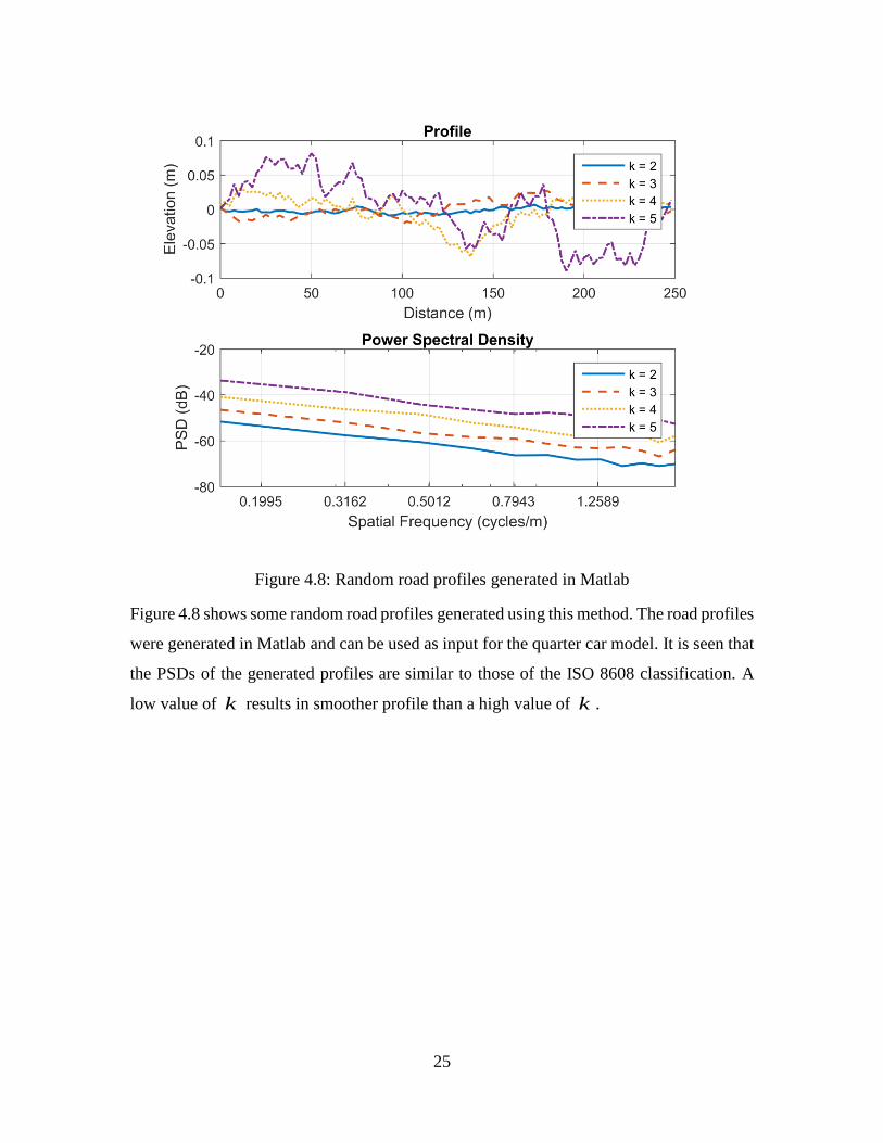
Figure 4.8 shows some random road profiles generated using this method. The road profiles
were generated in Matlab and can be used as input for the quarter car model. It is seen that
the PSDs of the generated profiles are similar to those of the ISO 8608 classification. A
low value of k results in smoother profile than a high value of k .
Page 34
26
Figure 4.9: Uneven road profiles
Using this method, Class A road unevenness was added to every standard road profile to
increase the realism of the simulation results. Random single-event obstacles were also
developed using a high k value of seven to represent very harsh road profiles of class F
Uneven Road A
Uneven Road B
Uneven Road C
Page 35
27
to be tested by themselves. Figure 4.9 shows the uneven road obstacle profiles created in
Matlab for simulation.
4.2 Pre-processing Road Profiles
The road obstacle profiles serve as input to the quarter-car model through the tire. If the
wavelength is smaller than two or three times the contact length and the model is assumed
to contact the road at a single point, geometric filtering of the profile becomes necessary.
This is done to account for the enveloping of obstacles at the contact patch.
4.2.1 Tandem Elliptical Cam Pre-Processing
The ‘Tandem Elliptical Cam Technique’ as described in [18] was used to process the road
profile, and parameter values were obtained from [19]. This enveloping model moves over
the actual road surface and generates an effective road surface description that serves as
input to the quarter-car model. Numerous simulation results with measurements have
shown the model to be valid in the scope of experiments.
Figure 4.10: Filtering of road profile
Source: Pacejka, H. (2006). Tire and Vehicle Dynamics, Butterworth-Heinemann. Used
under fair use 2016.
Page 36
28
Figure 4.10 shows the filtering of a road profile and obtaining a basic curve using an
elliptical cam. It is seen that the basic curve behaves as a filtered version of the actual road
profile.
Figure 4.11: Generation of basic curve
Source: Schmeitz, A. J. C. (2004). A Semi-Empirical Three-Dimensional Model of the
Pneumatic Tyre Rolling over Arbitrarily Uneven Road Surfaces. Institutional Repository,
Delft University of Technology: 320. Used under fair use 2016.
Figure 4.11 shows the generation of the basic curve using an ellipse defined by the shape
parameters ea , eb and ec , where ec is the ellipse exponent. The selection of these shape
parameters allows the modeling of different tires in accordance with experimental results.
The derivation of the equation for the basic curve is now discussed.
1
e ec c
e e
x z
a b
(4.5)
Equation (4.5) gives the equation of the ellipse in local coordinates x and z .
Page 37
29
1
1 1
e ec c
step
b e
e
hl a
b
(4.6)
Equation (4.6) gives the length bl of the elliptical basic curve where steph is the height of
the step.
1
1
e ec c
e e
e
xz b
a
(4.7)
Equation (4.7) gives the distance ez between the local x-axis and the ellipse.
1
0
1
e e
b step
c c
step
step e e b step step
e
step step
Z if X l X
X XZ h b b if l X X X
a
Z h if X X
(4.8)
Equation (4.8) gives the global vertical coordinates Z for the basic curve.
To obtain an effective road profile from an input road profile, two elliptical cams are used
in tandem.
Page 38
30
Figure 4.12: Tandem Elliptical Cams
Source: Schmeitz, A. J. C. (2004). A Semi-Empirical Three-Dimensional Model of the
Pneumatic Tyre Rolling over Arbitrarily Uneven Road Surfaces. Institutional Repository,
Delft University of Technology: 320. Used under fair use 2016.
The Figure 4.12 shows the tandem elliptical cams connected by an upper and lower tandem
rod. Upper case letters represent global coordinates while lower case letters represent local
coordinates. fX , fZ and rX , rZ represent the centers of the front and rear ellipse in global
coordinates and similarly for the lower case letters.
max ( )f road f f e fZ Z X x z x
(4.9)
Equation (4.9) gives the global height of the front ellipse center where roadZ is any input
road profile defined at distances fX . The global height of the rear ellipse is calculated in
the same way.
( )2
f r
e
Z Zw X b
(4.10)
Page 39
31
Equation (4.10) gives the effective height ( w ) which equals the midpoint of the lower
tandem rod. This equation can be used to obtain the final effective profile for any input
road profile.
0
0
2
sls
eae
ebe
ce e
lp
a
ap
r
bp
r
p c
(4.11)
Equations (4.11) give the dimensionless parameters which control the length of the tandem
rod and shape of the elliptical cam. It is assumed that the tandem base length ( )sl is related
to the contact length (2 )a of the tire and that the shape of the elliptical cam is related to
the free tire radius 0( )r .
Table 4.4: Chosen elliptical cam parameters for simulation
Source: Pacejka, H. (2006). Tire and Vehicle Dynamics, Butterworth-Heinemann.
Parameter Description Symbol Value
Unloaded Radius or 0.310 m
Effective rolling radius eor 0.305 m
Half contact length a 0.0603 m
Half ellipse length / unloaded radius aep 1.0325
Half ellipse height / unloaded radius bep 1.0306
Ellipse exponent cep 1.8230
Shift length / contact length shp 0.8773
Table 4.4 gives the chosen elliptical cam parameters for simulation. They can be modified
to obtain the effects of different tires and vehicle loads.
The ‘Tandem Elliptical Cam Technique’ can be used to process a road profile and obtain
an effective profile that can be used as input to the quarter-car model.
Page 40
32
Figure 4.13: Filtering of road profile using tandem elliptical cams
Matlab code was developed to pre-process any input road profile using this technique.
Figure 4.13 shows an example of the filtering effect of the ‘Tandem Elliptical Cam
Technique’. The original profile once filtered, gives a different effective profile.
4.2.2 Low-Pass Filtering
The profile once filtered using the ‘Tandem Elliptical Cam Technique’ still has
discontinuities due to the underlying road profile. These can cause spikes in the vertical
velocity input to the quarter-car model.
A first order Butterworth filter was used as a low-pass filter to reduce these discontinuities.
The break frequency was chosen to be 150 Hz, since the dynamics we were interested in
fall within this frequency.
Page 41
33
Figure 4.14: Processing of road profiles
Figure 4.14 shows the result of processing a road profile with both, the ‘Tandem Elliptical
Cam Technique’ and adding a low-pass filter to eliminate discontinuities. A smoother
profile is obtained.
4.2.3 Obtaining Vertical Velocity Profile
The obtained profile gives us the vertical displacement of the wheel as a function of
horizontal travel. However, the required input for the developed quarter-car model is a
vertical velocity profile as a function of time.
For a given vehicle velocity, the profile can be converted to vertical displacement as a
function of time. The vertical displacement was then differentiated with respect to time to
obtain a vertical velocity profile as a function of time. This serves as the unilateral boundary
condition for the quarter-car model.
Page 42
34
Figure 4.15: Unilateral boundary condition
Figure 4.15 shows the unilateral boundary condition for the quarter-car model obtained
using this method. For different vehicle velocities, the vertical displacement profile results
in different vertical velocity profiles.
Page 43
35
5 Optimized Control Force Estimation
Given a dynamic vehicle model, single-event road obstacle profile the aim of this research
is to determine the ideal control force profile to achieve the control objective. It is possible
to find this control force profile using offline optimization. Adaptive filtering is perfectly
suited to this task.
Adaptive filtering makes use of a cost function for optimization. The results of optimization
will depend on the chosen cost function for minimization. In the current problem of active
suspensions, adaptive filtering can be used to optimize either ride comfort, handling, or
minimize the rattle space. In the work presented here, ride comfort was chosen as the
objective. By changing the cost function, other objectives can also be achieved.
The performance indices relating ride comfort and handling are often measured by the root-
mean-square (RMS) values of sprung mass acceleration and tire deflection respectively
[28]. Therefore, the expected value of squared sprung mass acceleration was chosen as the
main parameter for the cost function given by (5.1) which needs to be minimized.
21( ) ( )c s
event
J F a t dtT
(5.1)
The method used for adaptive filtering is the Filtered-X-LMS algorithm, which is an
extension of the LMS optimization method.
5.1 LMS Optimization
The LMS optimization method [20] is used to obtain an ideal filter that can minimize the
error between its output signal and a desired signal.
Page 44
36
Figure 5.1: Adaptive linear combiner
Figure 5.1 shows a schematic diagram of an adaptive linear combiner. It is a time-varying,
non-recursive digital filter. There is an input signal vector ( )kX with elements (k L)x …
(k 1)x up to (k)x and a corresponding set of adjustable weights ( )kW with elements ( )o kw , 1( )kw
, … ( )L kw , a summing unit, and a single output signal ( )ku , where ( )k represent the kth
time index and L is the number of weights.
( ) ( ) ( )
0
L
k l k k l
l
u w x
(5.2)
For a fixed setting of the weights, the output is a linear combination of the inputs (5.2).
The output signal ( )ku is subtracted from the desired signal ( )kd to produce the error signal
( )k . The adaptation process is designed to reduce this error.
Page 45
37
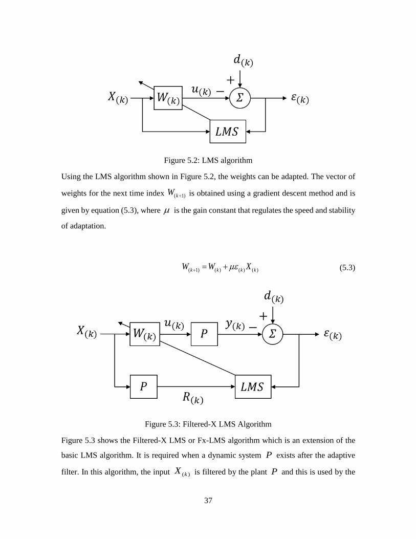
Figure 5.2: LMS algorithm
Using the LMS algorithm shown in Figure 5.2, the weights can be adapted. The vector of
weights for the next time index ( 1)kW is obtained using a gradient descent method and is
given by equation (5.3), where is the gain constant that regulates the speed and stability
of adaptation.
( 1) ( ) ( ) ( )k k k kW W X (5.3)
Figure 5.3: Filtered-X LMS Algorithm
Figure 5.3 shows the Filtered-X LMS or Fx-LMS algorithm which is an extension of the
basic LMS algorithm. It is required when a dynamic system P exists after the adaptive
filter. In this algorithm, the input ( )kX is filtered by the plant P and this is used by the
Page 46
38
LMS algorithm. The vector of weights for the next time index ( 1)kW is obtained using a
gradient descent method and is given by equation (5.4).
( 1) ( ) ( ) ( )k k k kW W R (5.5)
While the LMS algorithm is used for system modeling, the Fx-LMS algorithm works well
for inverse filtering. The Fx-LMS algorithm converges to de-correlate from d .
5.1.1 Iterative LMS Adaptation
Since the focus was on single-event obstacles, which are not persistent, an iterative batch
modification was required. When the Fx-LMS algorithm in Figure 5.3 is used on a batch
of input X , an optimized vector of weights W is obtained. The algorithm can then be used
again on the same batch of input, but this time, the W vector from the previous iteration
can be used as an initial condition. In this way, the vector of weights W is optimized further
in each iteration. This will be referred to as Iterative LMS adaptation.
Figure 5.4: Iterative LMS Adaptation of filter coefficients
Page 47
39
Figure 5.4 shows how the filter W gets optimized over each iteration. In this example, W
was chosen to have 35 coefficients and 25 iterations were used to obtain the final filter.
This illustrates how the Iterative LMS Adaptation works offline on the same batch of input
multiple times until the final filter W is obtained. This also enables a way to directly
evaluate convergence.
Figure 5.5: Iterative LMS Adaptation – poor performance
Figure 5.5 shows the Iterative LMS Adaptation for a randomly generated SISO plant model
P , a random input kx and a random desired response kd . It is seen that after running the
algorithm for 500 iterations, the mean square error between the desired response kd and
output ky reduces by 3.41 dB, which is not acceptable.
Page 48
40
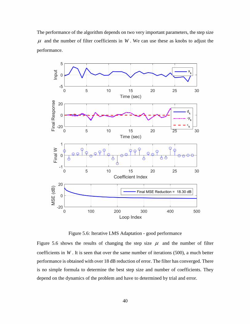
The performance of the algorithm depends on two very important parameters, the step size
and the number of filter coefficients in W . We can use these as knobs to adjust the
performance.
Figure 5.6: Iterative LMS Adaptation - good performance
Figure 5.6 shows the results of changing the step size and the number of filter
coefficients in W . It is seen that over the same number of iterations (500), a much better
performance is obtained with over 18 dB reduction of error. The filter has converged. There
is no simple formula to determine the best step size and number of coefficients. They
depend on the dynamics of the problem and have to determined by trial and error.
Page 49
41
Figure 3.3 shows the state space model of the quarter car. The paths between the road input
rz , the control effort cF and the sprung mass acceleration sa are the paths of interest.
The Iterative LMS Adaptation is used to develop a controller that applies the required
control effort that can de-correlate the sprung mass acceleration from the road input,
assuming an actuator with unlimited authority.
Figure 5.7: Fx-LMS algorithm applied to quarter-car model
Figure 5.7 shows the application of the iterative LMS Adaptation to the quarter-car model
where the original form of the Fx-LMS algorithm is shown for comparison. The road input
Page 50
42
is ( )r kz and is delayed by samples to give (k )rz which is applied to the quarter-car.
This mean that ( )r kz is effectively preview information for LMS adaptation. Using this
preview information, the adaptation is performed to optimize the adaptive filter coefficients
in ( )kW which produces the control effort ( )c kF for the plant P . The resulting sprung mass
acceleration ( )s ka due to the road disturbance ( )kd and control effort ( )c kF is the error
( )k , which will get de-correlated from the input after convergence. The simplified case is
assumed in which perfect knowledge of the system models and measured road input are
available.
The resulting control effort can be analyzed to determine the peak force and bandwidth
required to overcome the specific road obstacle profile.
5.2 FIR Filter Model
The state space model equations (3.5) are in continuous time and not suitable for Iterative
LMS Adaptation. The Fx-LMS algorithm is designed to work only with FIR filter models.
Finite Impulse Response (FIR) filters were chosen for discretizing the system.
FIR filters for each path in Figure 3.3 that represent the transfer functions for the system
were used to create the discrete model. An impulse response can be generated for each path
and this creates the FIR filter for the path.
Page 51
43
Figure 5.8: FIR filters for transfer function paths
Figure 5.8 shows the FIR filters that represent the quarter car model. There are two inputs,
namely the vertical velocity due to the road profile rz and the control effort cF . There are
also two outputs namely the sprung mass acceleration sa and suspension deflection .
Therefore there are four possible paths from inputs to outputs.
Page 52
44
Figure 5.9: Transfer functions for quarter-car model
Figure 5.9 shows the transfer function for each path. It is seen that the FIR filter discrete
model is a very good approximation of the continuous model.
5.2.1 Model Regeneration
The simulations were performed for different vehicle velocities. When the vehicle velocity
is increased, the input discrete road excitation takes a much shorter time as shown in Figure
5.10.
Page 53
45
Figure 5.10: Velocity input comparison
Therefore, a higher sample rate had to be used for higher velocities so that the discretized
vertical displacement accurately represents the original road profile input. The FIR filters
are only suitable for use at the sample rate at which they are generated. For this reason,
each time the vehicle velocity was changed, the FIR filters were re-generated for the new
sample rate.
Page 54
46
6 Results
A case study was conducted using Iterative LMS adaptation together with the discrete-time
quarter-car model to obtain the required control effort for different road obstacle profiles.
The continuous model was first created using the selected vehicle parameters.
A road profile was then selected for the case study. This road profile was sampled at a
chosen sampling rate which was low enough to not be too processor intensive and yet high
enough to accurately represent the geometry of the profile. A randomly generated road
profile based on ISO standards was added to the profile to better represent road conditions.
It was then processed with the ‘Tandem Elliptical Cam Technique’ to account for the
interaction of the tire with the profile and then filtered using a Butterworth filter to get rid
of discontinuities. This profile was then differentiated to obtain a vertical velocity profile
that served as input to the quarter-car model.
Having selected a sampling rate for the profile, the continuous quarter-car model was used
to obtain a discrete model at this sampling rate with FIR filters that had enough coefficients
to accurately represent the quarter-car dynamics.
Iterative LMS adaptation was used to obtain the ideal control effort to de-correlate the
system response from the road obstacle input.
Page 55
47
Figure 6.1: Iterative LMS Adaptation applied to quarter-car
Figure 6.1 shows the development of a filter for a quarter-car using Iterative LMS
Adaptation. The input to the model is shown in the first plot. It was a pothole at a low
velocity represented by the blue curve ( )r kz . Preview information for LMS adaptation is
represented by the green curve ( )r kz . The output due to the road obstacle profile is d ,
while the output due to the control effort applied to the plant is y . The difference between
them is the resulting sprung mass acceleration sa , or the error which needs to be reduced.
The mean square error (MSE) was compared between the sprung mass acceleration with
control and without control. It is directly related to the root-mean-square value of sprung
Page 56
48
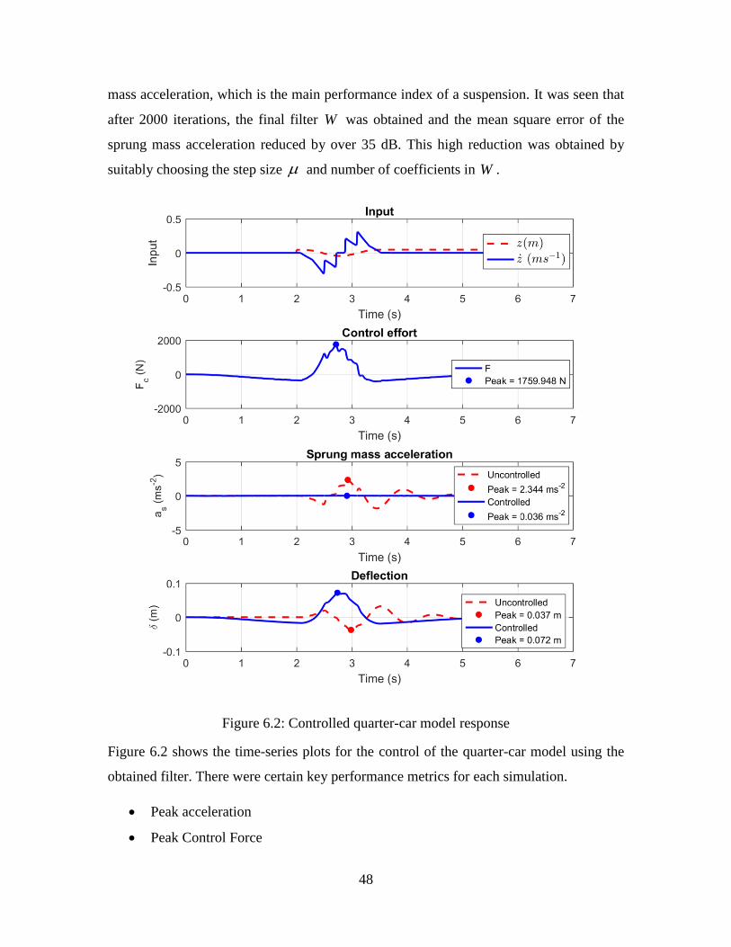
mass acceleration, which is the main performance index of a suspension. It was seen that
after 2000 iterations, the final filter W was obtained and the mean square error of the
sprung mass acceleration reduced by over 35 dB. This high reduction was obtained by
suitably choosing the step size and number of coefficients in W .
Figure 6.2: Controlled quarter-car model response
Figure 6.2 shows the time-series plots for the control of the quarter-car model using the
obtained filter. There were certain key performance metrics for each simulation.
Peak acceleration
Peak Control Force
Page 57
49
Bandwidth
Peak Deflection
The sprung mass acceleration sa was drastically reduced and the peak acceleration can be
obtained from the plot of sprung mass acceleration in Figure 6.2 . The plot of control effort
cF is shown and is used to obtain the peak force. The suspension deflection is also
obtained and can be used if the control goal changes from ride comfort. The bandwidth can
be obtained from the PSD of the control force profile.
Figure 6.3: 80% Power Bandwidth
Figure 6.3 shows the PSD of the control effort. The bandwidth is not evident from the plot
since there is no easily determined -3dB point. Instead, a plot of frequency versus the
percentage of total power is used to find the frequency within which 80% of the total power
is present. This is approximately equivalent to the -3dB frequency of a 2nd order low pass
filter and is a good metric for the bandwidth.
Page 58
50
1
1
(i)
(J) : 0.8,
(i)
J
i
N
i
PSD
P f J
PSD
(6.1)
This will be referred to as the 80% Power Bandwidth and is given by equation (6.1) where
( )f J is the frequency at frequency bin J and N is the total number of frequency bins
for the PSD. We see that for the chosen input, more than 80 percent of the total power is
below 11 Hz represented by the red line.
The simulation was run for each unique road input with multiple combinations of vehicle
velocities and preview distances as shown in Table 5. Nine hundred simulations were
performed in total.
Table 5: Simulation Conditions
Road Profile Preview Distance (m) Vehicle Velocity (mph)
Speed Hump Watts Profile 0 5
Speed Hump Seminole Profile 0.5 10
Curb A 1 15
Curb B 1.5 20
Curb C 2 25
Curb D 30
Curb E 35
Curb F 40
Curb G 50
Uneven Road A 60
Uneven Road B 70
Uneven Road C 80
Pothole P1
Pothole P6
Pothole P9
The simulations were run for realistic preview information ranging from no look-ahead
preview, to look ahead preview of two meters ahead. It should be noted that although look
ahead preview is practically realized as a distance, it is helpful to the algorithm because of
the additional time steps available for adaptation. In [12] it was found that preview times
of even 0.2 s were valuable. However, even the maximum preview distance of two meters
translates to only 0.4474 s at a low velocity of 10 mph and 0.056 s at a high velocity of 80
Page 59
51
mph. Therefore, at high velocities, the look ahead preview has a negligible effect. It was
also found in [16] that preview information results in no improvement past a certain time,
approximately 0.5 s. This maximizes the use of preview at low vehicle velocities for the
work presented in this thesis at a preview distance of 2 m.
Figure 6.4: Peak force surface for non-converged filter W
It was found that, when a non-converged filter W was used, the performance of the control
effort was poor. For this undesirable condition, preview distance had a high impact on the
results of the simulation since it was used to improve the performance. This is shown in
Figure 6.4.
Page 60
52
Figure 6.5: Peak force surface for converged filter W
Figure 3.1 shows the results of simulation when a properly converged filter W was used.
The preview distance did not have much of an effect.
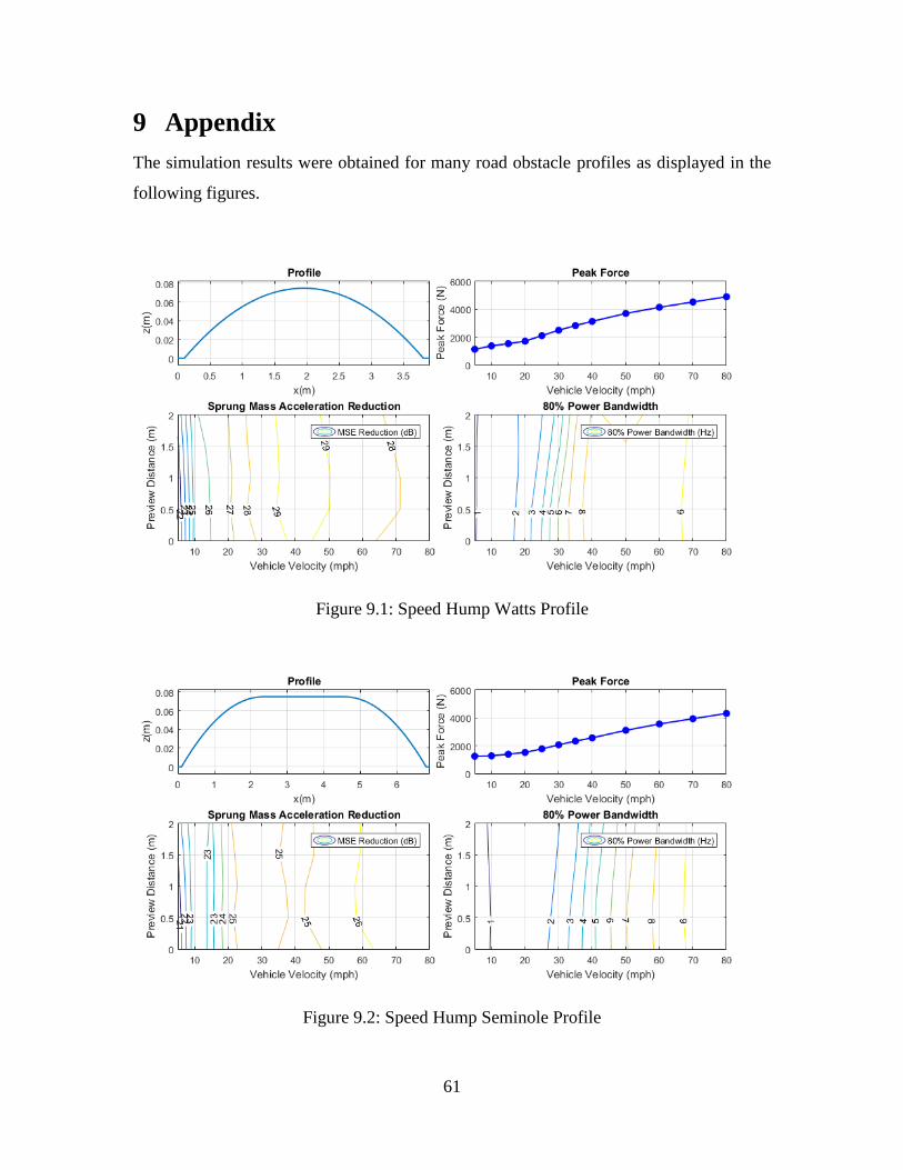
The results are presented for four of the types of profiles of importance. The complete set
of results are in the Appendix.
Page 61
53
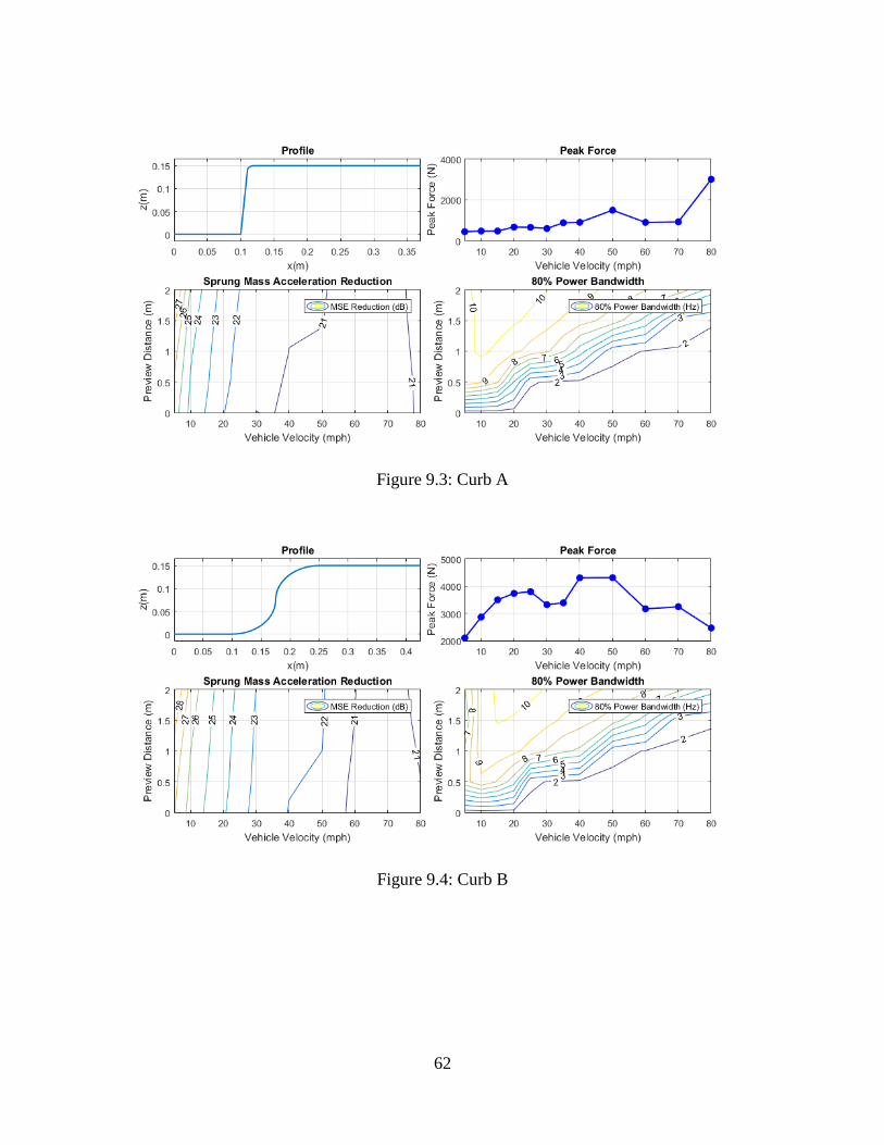
6.1.1 Case study results: Curb A
Figure 6.6: Results for Curb A
The simulations were performed for the ‘Curb A’ profile. Figure 6.6 shows the peak force
and bandwidth for different vehicle velocities and preview distances. Peak force
requirement generally increases as the vehicle velocity increases. There is a minor effect
of preview distance on the sprung mass acceleration reduction. At higher velocity, the
sprung mass acceleration reduction decreases. However, it is always over 20 dB which
means that the ideal control-force profile performs very well. Higher bandwidth is required
at lower velocities and high preview distances.
Page 62
54
6.1.2 Case study results: Pothole P1
Figure 6.7: Results for Pothole P1
The simulations were performed for ‘Pothole P1’. Figure 6.7 shows the peak force and
bandwidth for different vehicle velocities and preview distances. For the pothole, the peak
force increases initially and reduces at higher velocities. The preview distance does not
have much effect on the sprung mass acceleration reduction or bandwidth requirements.
At higher velocities, the sprung mass acceleration reduction reduces. The performance of
the ideal control-force profile is always good, with over 14 dB of sprung mass acceleration
reduction in all cases.
Page 63
55
6.1.3 Case study results: Speed Hump Watts Profile
Figure 6.8: Results for Speed Hump Watts Profile
The simulations were performed for a speed hump with a Watts Profile. Figure 6.8 shows
the peak force and bandwidth for different vehicle velocities and preview distances. For
the speed hump, the peak force increases as the vehicle velocity increases. The preview
distance does not have much effect on the sprung mass acceleration reduction. At higher
velocities, the sprung mass acceleration reduction reduces. The performance of the ideal
control force is very good with over 28 dB of reduction in all cases. The preview distance
does not have much of an effect on the bandwidth requirements.
Page 64
56
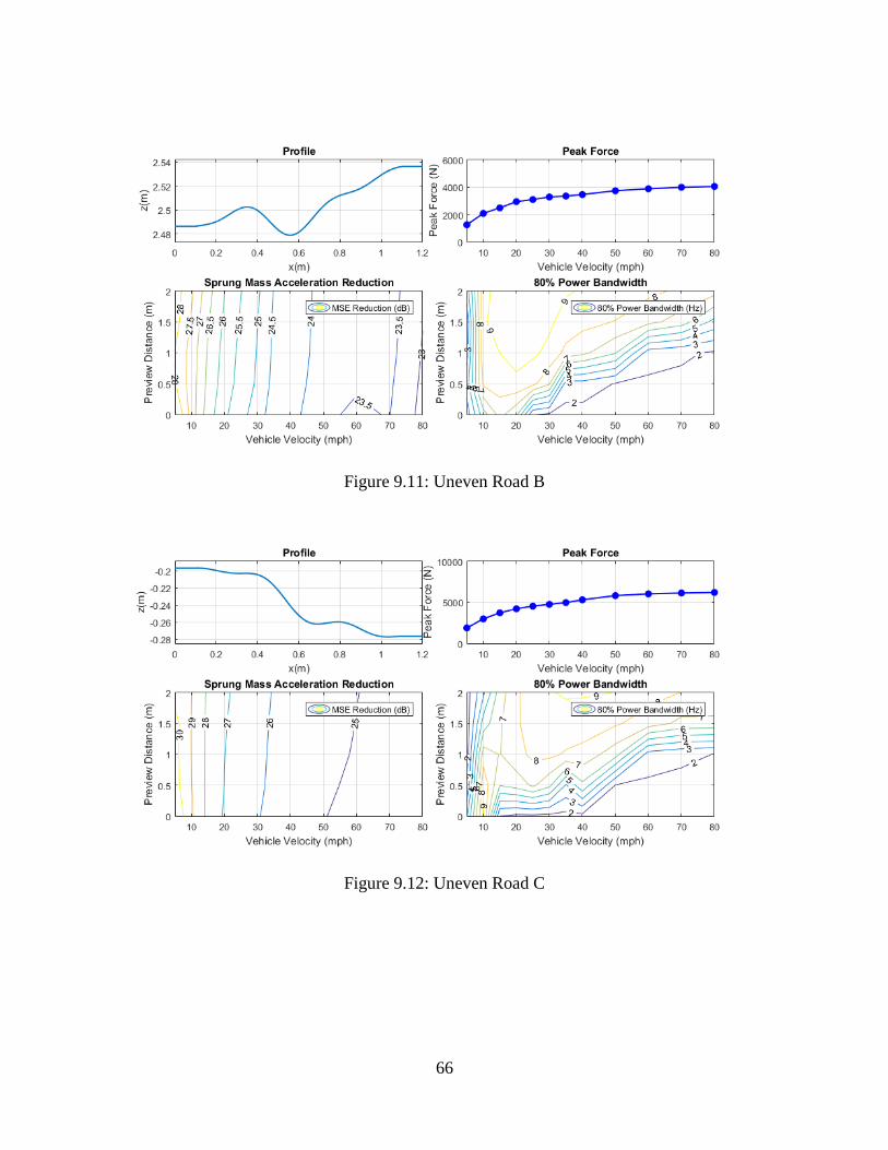
6.1.4 Case study results: Uneven Road A
Figure 6.9: Results for Uneven Road A
The simulations were performed for ‘Uneven Road A’, which is of very poor quality (class
F). Figure 6.7 shows the peak force and bandwidth for different vehicle velocities and
preview distances. For the uneven road profile, the peak force increases as the vehicle
velocity increases. The preview distance does not have much effect on the sprung mass
acceleration reduction. At higher velocities, the sprung mass acceleration reduction
reduces. The performance of the ideal control force is very good with over 24 dB of
reduction in all cases. Higher bandwidth is required at certain velocities and high preview
distances. This suggests that the characteristics of the obstacle influence the required
bandwidth more at certain vehicle velocities.
Page 65
57
7 Conclusions
The peak force requirement depends on the vehicle velocity and profile characteristics or
excitation. The bandwidth requirements are affected by the velocity of the vehicle and
look-ahead preview.
This research showed that vehicle velocity has a much greater effect on peak force and
bandwidth than look-ahead preview, but the trend depends on the profile.
For this study, the effects of look-ahead preview appears to only depend on convergence
and numerical issues.
The developed processing method using the ‘Tandem Elliptical Cam Technique’ and
filtering were easily applied to all types of road profiles and gave results similar to those
applied in practical testing from literature [18].
The ideal control force profile obtained with the help of Iterative LMS adaptation
performed very well regardless of the road obstacle profile and velocity of the vehicle in a
consistent manner, with over 18 dB of reduction in sprung mass acceleration in all cases.
7.1 Contributions
The iterative LMS adaptation method was developed to determine the ideal control effort
which was shown to be very effective at de-correlating the response of a quarter-car from
a known single-event excitation.
A discrete quarter-car model well suited to the iterative LMS adaptation method was
developed.
A database of twelve single-event road obstacle profiles including road unevenness was
created based on standards and existing literature.
The ‘Tandem Elliptical Cam Technique’ was used to account for the enveloping effect of
tires and represent road-tire interaction more accurately.
Case studies were performed by simulating the response of the developed quarter-car
model using different road obstacles. The results were used to determine the peak force
Page 66
58
and bandwidth of the required actuation. The developed method is generalized and allows
for modification in the system model and boundary conditions.
7.2 Future Work
The quarter-car model can be extended to a full-vehicle model to allow for more realistic
simulations of vehicles due to rolling and pitching and also more actuators for active
suspension control. Iterative LMS Adaptation can also be applied to higher degree of
freedom models.
Along with increasing the variety of road obstacles, non-unilateral boundary conditions
such as soft soil or road breakaway could be developed to improve the simulation of road-
tire interaction.
The results of simulation can be used to design actuators well suited to the control of active
suspensions. The Quarter-car testing rig developed by Justin Langdon [29] can be used for
practical testing of a custom built actuator with the control effort obtained through Iterative
LMS Adaptation.
Page 67
59
8 References
1. Tseng, H.E. and D. Hrovat, State of the art survey: active and semi-active suspension
control. Vehicle System Dynamics, 2015. 53(7): p. 1034-1062.
2. Sharp, R.S. and D.A. Crolla, Road Vehicle Suspension System Design - a review.
Vehicle System Dynamics, 1987. 16(3): p. 167-192.
3. Gysen, B.L., et al., Active electromagnetic suspension system for improved vehicle
dynamics. IEEE Transactions on Vehicular Technology, 2010. 59(3): p. 1156-1163.
4. Weeks, D., et al., The design of an electromagnetic linear actuator for an active
suspension. 1999, SAE Technical Paper.
5. Iijima, T., et al., Development of a hydraulic active suspension. 1993, SAE Technical
Paper.
6. Ghazaly, N.M. and A.O. Moaaz, The Future Development and Analysis of Vehicle
Active Suspension System. IOSR Journal of Mechanical and Civil Engineering, 2014.
11(5): p. 19-25.
7. Thompson, A., An active suspension with optimal linear state feedback. Vehicle system
dynamics, 1976. 5(4): p. 187-203.
8. Ting, C.-S., T.-H.S. Li, and F.-C. Kung, Design of fuzzy controller for active suspension
system. Mechatronics, 1995. 5(4): p. 365-383.
9. Nguyen, T.T., et al. A hybrid control of active suspension system using H∞ and nonlinear
adaptive controls. in Industrial Electronics, 2001. Proceedings. ISIE 2001. IEEE
International Symposium on. 2001. IEEE.
10. Munari, L.A., et al., Retrieving Road Surface Profiles from PSDs for Ride Simulation of
Vehicles. 2012, SAE Technical Paper.
11. Dodds, C. and J. Robson, The description of road surface roughness. Journal of sound
and vibration, 1973. 31(2): p. 175-183.
12. Bender, E.K., Optimum Linear Preview Control With Application to Vehicle Suspension.
Journal of Basic Engineering, 1968. 90(2): p. 213-221.
13. Tomizuka, M., “Optimum Linear Preview Control With Application to Vehicle
Suspension”—Revisited. Journal of Dynamic Systems, Measurement, and Control,
1976. 98(3): p. 309-315.
14. Louam, N., D. Wilson, and R. Sharp, Optimal control of a vehicle suspension
incorporating the time delay between front and rear wheel inputs. Vehicle system
dynamics, 1988. 17(6): p. 317-336.
15. Adibi Asl, H. and G. Rideout. Using lead vehicle response to generate preview functions
for active suspension of convoy vehicles. in American Control Conference (ACC), 2010.
2010.
16. Hać, A., Optimal linear preview control of active vehicle suspension. Vehicle system
dynamics, 1992. 21(1): p. 167-195.
17. Agostinacchio, M., D. Ciampa, and S. Olita, The vibrations induced by surface
irregularities in road pavements - a Matlab approach. European Transport Research
Review, 2014. 6(3): p. 267-275.
Page 68
60
18. Schmeitz, A.J.C., A Semi-Empirical Three-Dimensional Model of the Pneumatic Tyre
Rolling over Arbitrarily Uneven Road Surfaces. 2004, Delft University of Technology:
Institutional Repository. p. 320.
19. Pacejka, H., Tire and Vehicle Dynamics. 2 ed. 2006: Butterworth-Heinemann. 672.
20. Bernard Widrow, S.D.S., Adaptive Signal Processing. 1985: Prentice Hall. 475.
21. Song, X., et al., An Adaptive Semiactive Control Algorithm for Magnetorheological
Suspension Systems. Journal of Vibration and Acoustics, 2005. 127(5): p. 493-502.
22. Plaxico, C.A., et al., Recommended Guidelines for Curb and Curb-Barrier Installations.
2005: United States. p. 112p.
23. Parkhill, M., R. Sooklall, and G. Bahar. Updated guidelines for the design and
application of speed humps. in Institute of Transportation Engineers Annual Meeting and
Exhibit 2007, August 5, 2007 - August 8, 2007. 2007. Pittsburgh, PA, United states:
Institute of Transporation Engineers.
24. Weber, P.A. and J.P. Braaksma, Towards a North American geometric design standard
for speed humps. ITE Journal (Institute of Transportation Engineers), 2000. 70(1): p.
30-34.
25. Miller, J.S. and W.Y. Bellinger, Distress identification manual for the long-term
pavement performance program. 2003.
26. Tiong, P.L.Y., M. Mustaffar, and M.R. Hainin, Road surface assessment of pothole
severity by close range digital photogrammetry method. World Appl Sci J, 2012. 19(6):
p. 867-873.
27. Kropáč, O. and P. Múčka, Classification scheme for random longitudinal road
unevenness considering road waviness and vehicle response. Shock and Vibration, 2009.
16(3): p. 273-289.
28. Hrovat, D., Survey of advanced suspension developments and related optimal control
applications. Automatica, 1997. 33(10): p. 1781-1817.
29. Langdon, J.D., Design and Adaptive Control of a Lab-based, Tire-coupled, Quarter-car
Suspension Test Rig for the Accurate Re-creation of Vehicle Response, in Mechanical
Engineering. 2007, Virginia Polytechnic Institute and State University. p. 124.
Page 69
61
9 Appendix
The simulation results were obtained for many road obstacle profiles as displayed in the
following figures.
Figure 9.1: Speed Hump Watts Profile
Figure 9.2: Speed Hump Seminole Profile
Page 70
62
Figure 9.3: Curb A
Figure 9.4: Curb B
Page 71
63
Figure 9.5: Curb C
Figure 9.6: Curb D
Page 72
64
Figure 9.7: Curb E
Figure 9.8: Curb F
Page 73
65
Figure 9.9: Curb G
Figure 9.10: Uneven Road A
Page 74
66
Figure 9.11: Uneven Road B
Figure 9.12: Uneven Road C
Page 75
67
Figure 9.13: Pothole P1
Figure 9.14: Pothole P6
Page 76
68
Figure 9.15: Pothole P9