A uthor .... LIBRARIES ........... ......... I........Department of Mechanical Engineering
August 4, 2000
-m /
Certified by......Jean-Jacques E. Slotine
Professor of Mechanical Engineering and Information SciencesProfessor of Brain and Cognitive Sciences
Thesis Supervisor
A ccepted by ...........................Ain A. Sonin
Chairman, Department Committee on Graduate Students
. -. ..........
A Study of Contraction Theory and Oscillatorsby
Caroline Combescot
Submitted to the Department of Mechanical Engineeringon August 4, 2000, in partial fulfillment of the
requirements for the degree ofMaster of Science in Mechanical Engineering
Abstract
Oscillators have been the subject of numerous studies recently, as they show a veryfascinating synchronizing behavior. But most of the results are relying on simulationsand very few theoretical results have been derived to show this behavior. Recently,Jean-Jacques Slotine and Winfried Lohmiller developed in the Nonlinear SystemsLaboratory a new analysis of non linear systems, called Contraction Theory, whichstudies the stability of a system with respect to a trajectory. This thesis uses thisnew approach to study the behavior of classes of nonlinear systems defined by anequation derived from the linearly damped oscillator. Theoretical proofs of somesynchronization behaviors can then be derived in a fairly simple manner compared towhat is done in the to date literature of the theory of oscillators.
Thesis Supervisor: Jean-Jacques E. SlotineTitle: Professor of Mechanical Engineering and Information Sciences; Professor ofBrain and Cognitive Sciences
3
Acknowledgments
I would like to thank very deeply all the people that enabled me to go through thiswork: My advisor Jean-Jacques Slotine for providing support and leading me thewhole way in my research. My lab mates and friends Alex, Lutz, Martin, Winni,Emilio, Jeff, Danielle, and last but not least Gilles, as well as my family, for beingthere to discuss any kind of matter and help me keep the right direction.
This work was supported in part by grant NSF/KDI 6777400.
5.5 Contraction study of the damped van der Pol using a change of variables 595.5.1 Introduction . . . . . . . . . . . . . . . . . . . . . . . . . . . . 595.5.2 Change of variables . . . . . . . . . . . . . . . . . . . . . . . . 595.5.3 Contraction study . . . . . . . . . . . . . . . . . . . . . . . . . 60
5.6 Weak Contraction study of the damped van der Pol . . . . . . . . . 635.6.1 Introduction . . . . . . . . . . . . . . . . . . . . . . . . . . . . 635.6.2 Weak contraction study . . . . . . . . . . . . . . . . . . . . . 635.6.3 Expression of the change of variables as a e matrix . . . . . . 65
6 Proved synchronization behaviors of combinations of van der Poloscillators 676.1 Synchronization of van der Pol oscillators . . . . . . . . . . . . . . . . 67
6.1.1 Tuning of two van der Pol oscillators . . . . . . . . . . . . . . 676.1.2 Synchronization of n + 1 van der Pol oscillators . . . . . . . . 69
6.3 Operations with van der Pol oscillators . . . . . . . . . . .6.3.1 Addition of two van der Pol oscillators . . . . . . .6.3.2 Addition of n van der Pol oscillators . . . . . . . .6.3.3 Multiplication by a constant . . . . . . . . . . . . .
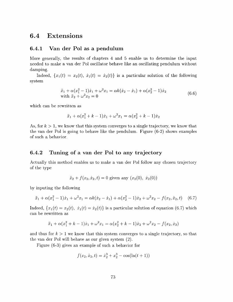
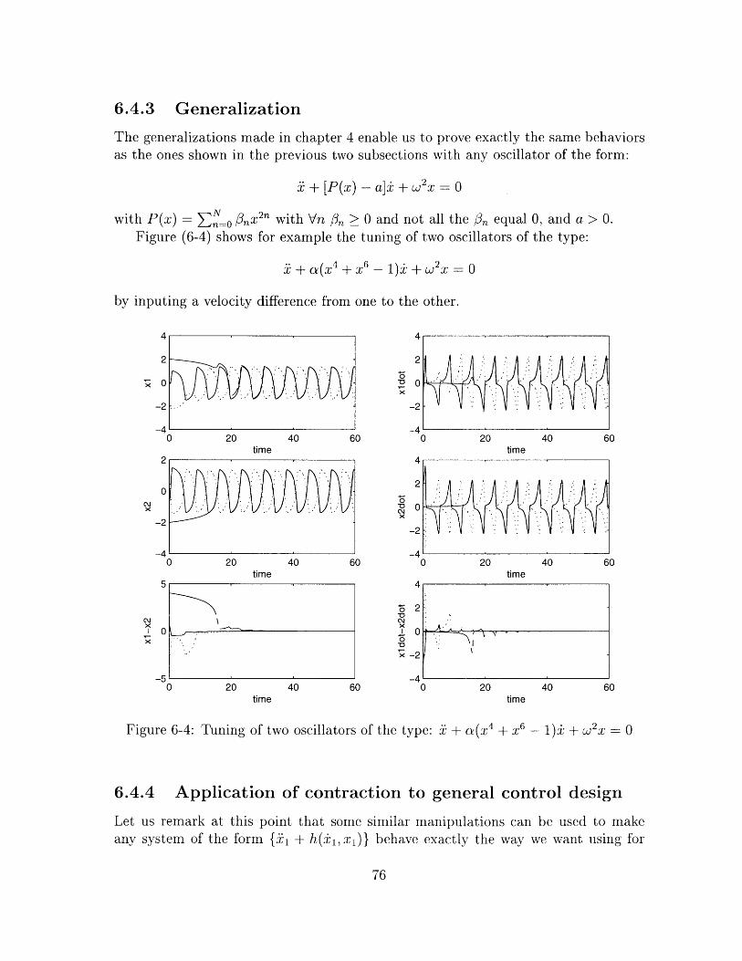
6.4 Extensions . . . . . . . . . . . . . . . . . . . . . . . . . . .6.4.1 Van der Pol as a pendulum . . . . . . . . . . . . .6.4.2 Tuning of a van der Pol to any trajectory . . . . . .6.4.3 Generalization . . . . . . . . . . . . . . . . . . . . .6.4.4 Application of contraction to general control design
6.5 Feedback Combination of two van der Pol oscillators . . .
7
7 Conclusion
. . . . . . 70
. . . . . . 70
. . . . . . 71
. . . . . . 72
. . . . . . 73
. . . . . . 73
. . . . . . 73
. . . . . . 76
. . . . . . 76
. . . . . . 77
81
8
Chapter 1
Introduction
Oscillators govern a lot of physiological and biological rhythmic motions, enablingsynchronization of periodic oscillations in a noisy and disturbed environment. Ex-amples go from heartbeat in our body, to control of a humanoid arm, achieved byMatthew Williamson recently at MIT. So far very few theoretical results on stabilityof systems controlled by oscillators have been shown.
The approach used in Contraction Theory is aimed to derive results on the stabilityof a system with respect to a trajectory, it does not depend on the particular timedependent input that is governing the system. Therefore changing the time dependentinput function does not alter the stability result derived. Contraction Theory can thusbe used to get a better understanding of how systems remain stable with very fewrequirements on the knowledge of the environment, which may be characterized asno requirements on the input to the system.
This thesis uses such an approach to derive theoretical results on behaviors ofnonlinear systems derived from the damped pendulum, and then prove the synchro-nization of certain types of oscillatory systems. Chapter 2 gives a general view ofthe motivation for studying oscillators. It ends by describing the synchronizationbehavior that triggered the interest in the systems studied in this thesis. Chapter 3introduces Contraction Theory. It derives some intuitive and geometric explanationsof the mathematics involved, and gives an example to get better hands on understand-ing of how this theory can be applied. Chapter 4 gives a mathematical demonstrationof the contraction behavior of a certain class of nonlinear system derived from thedamped pendulum. Chapter 5 derives different types of use of metrics to get contrac-tion results on systems of interest. It ends up with a weak contraction study of thedamped van der Pol which gives us contraction for this system. Chapter 6 uses someof the previously derived theoretical results to prove some synchronization behaviorsof interest. Finally, chapter 7 concludes on the work done.
9
10
Chapter 2
Oscillators
2.1 Introduction
2.1.1 Biological motivation
Oscillations are ubiquitous, in Mechanics as well as in Biology. In Biology almost allvital functions include in some way oscillations. Locomotion, be it using legs, wingsor fins, is rhythmic. Other familiar examples include breathing and heartbeat. Oursensory and nervous system depend on periodic oscillations to perform many of theirtasks.
In nature, coupled neurons constitute the basic oscillators. In a real biologicalsystem, one will never encounter an oscillator alone, as its signal would be too weakto provoke any motor or other behavior of interest to us. In animals, oscillators tendto occur clustered and interconnected in so-called Central Pattern Generators (CPGs)that oscillate in synchrony and thus produce output signals that are strong enoughto actually influence the targeted part of the nervous system or muscle. These seemto be at the core of all biological rhythmic activity. Examples for Central PatternGenerators are pacemaker cells in the heart, or groups of nerve cells in the spinal cordthat actuate legs in a rhythmic fashion.
2.1.2 The van der Pol equation
To simulate coupled neurons a wide variety of models have been derived. One of themost important equation among those is the van der Pol equation. This equation wasdiscovered by van der Pol while studying the "tetrode multivibrator" circuit used inearly radios. This circuit connects in parallel a magnetic coil and a capacitor, betweenwhich the energy swings periodically back and forth, as well as a non-linear resistor.The latter acts like an ordinary resistor for high voltages but for voltages below aspecific threshold, it reverses its behavior and the resistance becomes negative. Thiscan for example be realized by a twin-tunnel-diode circuit. This means that for high
11
voltages the system is damped down, whereas for low values, additional energy isinjected. Intuitively this should lead to a sustained oscillation at some intermediatevoltage.
For a general non-linear resistor with the voltage-controlled i - v characteristici = F(v), Kirchhoff's current laws yield the circuit equation
+ av F(v) + v = 0.
When F(v) = -v + !i the equation takes on the form3
1 + a,(v 2 - 1) + v = 0
which is known as the van der Pol (vdP) equation.
A more general form of the van der Pol equation can be written as follows
+ 2- 1)i + 2X = 0
Here w represents the natural frequency of the oscillation and a is a parameter whosesize has a very strong influence on the dynamics of the system.
The van der Pol equation has a stable limit cycle, whose existence can be provenfor a > 0 using the Poincare-Bendixson theorem. It can also be shown that the limitcycle is the unique solution aside from the trivial solution x 0, the unstableorigin [3].
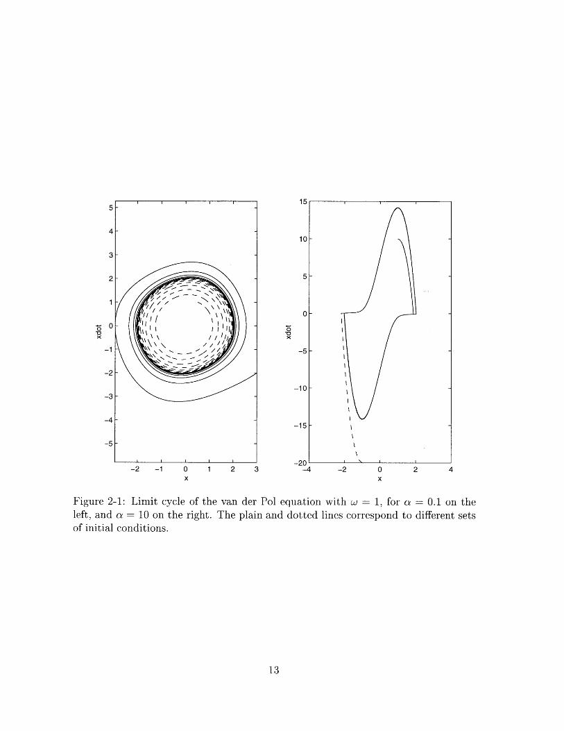
For small a the limit cycle in the (x, ±) plane looks like a circle with radius 2.For larger a the limit cycle is heavily distorted as the effect of the damping is morepronounced, thus its effects can be more easily observed. For JxJ > 1 the dampingis positive and large, and every increase in iJJ is heavily penalized. At JxJ = 1 thedamping changes its sign and turns into a forcing, thus accelerating the system forall JxJ < 1. This behavior can be seen on figure (2-1).
2.2 Van der Pol synchronization
There is a wide variety of synchronization behaviors of oscillators. One that kept ourattention is the following:
If a given van der Pol oscillator (1) is controlled by the difference of velocitybetween his velocity and the one of another identical van der Pol (2), vdP(1) will endup following the exact same trajectory as vdP(2).
This can be mathematically expressed by:
zi + a(Xz - 1)i + w2 x1 = ak(±2 - XI) with any (xi(0), Ji(0)) givenwith x2 verifying i 2 + a(xj - )d2 + W2x 2 = 0 and any (x2 (0), ±2(0)) given
12
5
4
3
2
1
0
-1
-2
-3
-4
-5
-2 -1 0 1 2 3
Figure 2-1: Limit cycle of the van der Pol equation with w = 1, forleft, and a = 10 on the right. The plain and dotted lines correspondof initial conditions.
a = 0.1 on theto different sets
13
+--
15
10
5
0
-5
-10
-15
-20-4 -2 0
x2 4
leads to x, converges to x2. In other words, x1 and x2 will end up on the same point ofthe limit cycle of the van der Pol. We thus end up with two exactly identical systems,oscillating at the same frequency, whatever initial conditions of the two systems.
Figure (2-2) shows examples of such a behavior.
0 10 20 30 4time
0 10 20 30 4time
10 20time
0
X
2
-2
0
2
0_0C\1
0
0
*0
30 40
0
-2
-4
5
0
-5
-10'0
0 10 20 30 4time
0 10 20 30 4time
10 20time
30 40
Figure 2-2: Convergence of vdP(1) to vdP(2). (a = 1, w = 1, k = 2)
Looking at the equations, we remark that the system actually converges to whatan obvious particular solution is. Thus, to prove this synchronization in a rigorousmanner, we need to show that the system will converge to a unique trajectory what-ever initial conditions it starts with. Indeed, in such a case, as there is one trajectorywhich is obvious if the system starts with the right initial conditions, we can concludethat the system will always converge to this trajectory.
This is exactly the kind of results that Contraction Theory enables to prove. Wetherefore introduce this new theory in the next chapter, before we use it to studythe contraction behavior of a variety of systems in the following two chapters. Theseresults enable us to go back to this synchronization behavior in chapter 6, and proveit, as well as derive proofs for other types of synchronization.
14
/V
4
2
-4
5
0
-5
-10
10
5
V.
0
C',JX0
-1010
0
4
C\JX
Chapter 3
Contraction Theory
This chapter exposes the main concepts of Contraction Theory [8], and tries to giveinsight in the mathematical formulae, by detailing the geometrical point of view, andgiving an example of use.
3.1 Definition and Basic result
Intuitively, contraction analysis is based on a slightly different view of what stabilityis. Regardless of the exact technical form in which it is defined, stability is generallyviewed relative to some nominal motion or equilibrium. Contraction analysis is mo-tivated by the elementary remark that talking about stability does not require one toknow what the nominal motion is.
3.1.1 Contracting systems
Let us consider a system in the form
f(x, t) (3.1)
where f is a n x 1 vector function, continuously differentiable, and x is the n x 1 statevector.
We define the Jacobian matrix J(x, t)
The main result of Contraction Theory is that in a region where the symmet-ric part of the Jacobian matrix is negative definite, the system convergesexponentially to a single trajectory, which does not depend on the initialconditions of the system within this region. The system is then called acontracting system in that region.
15
In particular, Contraction Theory enables to prove that the system will follow aparticular obvious trajectory if such a trajectory exists.
3.1.2 Justification
The proof of this result is the following. The virtual displacement 6x is an infinites-imal displacement at fixed time, thus 6xT6x characterizes the distance between twoneighboring trajectories.differentiating (3.1):
The dynamic of the virtual displacement is obtained by
(3.2)
which leads us to the dynamic of the distance between two neighboring trajectories:
d J+± Td-(6xT6x) = 6T6x + xT5& =2 6xT( jxdt 2
Defining A)max(x, t) the largest eigenvalue of the symmetric part of J, we can write
The symmetric part of the Jacobian being negative definite, we have 3 / >0 such that Vx, V t, Amax(X, t) < -0 < 0, i.e. Amax(X, t) is uniformly strictly nega-tive. Thus we have
|6x| ||x6 0| e--t
and 116xll converges to 0 exponentially.
3.1.3 Remarks
An important point is that one has to guarantee that a trajectory stays in the con-tracting region of the system, to be able to say that this trajectory is going to convergeto the single trajectory of that region. Indeed, the contracting behavior of a system
16
6,+ = J(X, t) 6X
Amax (X t) dt #
within a certain region, does not guarantee that any trajectory, starting in that re-gion, will remain in the region. And thus this has to be shown.
Something that should be pointed out too is the strength of the Contractionproperty. Indeed, if a system i f(x, t) is contracting in a certain region, then forany function of time u(t), the system i = f(x, t) + u(t) is also contracting. So twothings should always be kept in mind:
* If a system might intuitively have a contraction behavior with no input, oneshould always be careful to try to apprehend how would the system behave withsome type of time dependent input, which could alter the contracting behaviorintuition. As an example, let us consider a system which, with no input, has astable equilibrium point. Thus this system, with no input, converges to a singletrajectory -which in this case is a point- independent of the initial conditions.It is easy to understand that this does not imply, in the general case, that thissystem is going to converge to a single trajectory when the system is input atime dependent function u(t). This highlights the fact that Contraction is anotion different from Stability -as a matter of fact, a contracting system canvery well follow a diverging (non stable) trajectory.
* And on the other hand, if a system, already when there is no input, has obviouslya behavior (trajectory) which depends on the initial conditions, it is for surenot contracting. An example is the linear pendulum with no damping. Theeasy study of this system with no input, shows that the trajectory followed istotally dependent on the initial conditions. This should again give a feeling thatContraction is a particular property, that might not be satisfied even for verysimple systems.
The last important remark is that, with the use of a differential approach, convergenceanalysis and limit behavior are in a sense treated separately. Guaranteeing contractionmeans that after exponential transients, the system's behavior will be independent ofthe initial conditions.
In an observer context, one then needs only to verify that the observer equationscontain the actual plant state as a particular solution, to automatically guarantee con-vergence to that state. In a control context, once contraction is guaranteed throughfeedback, specifying the final behavior reduces to the problem of shaping one partic-ular solution, i.e., specifying an adequate open-loop control input to be added to thefeedback terms, a necessary step of any control method.
17
3.2 Advanced derivations
3.2.1 Generalization
The result stated in the previous section can be extended by using a more generaldefinition of distance between two trajectories.
This is done by defining a differential change of base
6Z = 196x
where e(x, t) is a square invertible matrix. By differentiating such an expression weget:
6i = 66x + &x =_ (6 + EJ)E)--6z = Fz (3.3)
This equation has the same form as (3.2). Thus, with the same reasoning as inthe previous section, we have the following result:
If the generalized Jacobian F = (E+EJ)E-1 is uniformly negative def-inite in a certain region, 116zlI, and thus ||6xfl, converges exponentially to 0 inthat region, and thus the system converges exponentially to a single trajec-tory, regardless of the initial conditions within this region.
We can get an equivalent result by defining M = E8T. The metric M(x, t) is asymmetric positive definite matrix representing the change of base from the distancepoint of view. We shall assume M to be uniformly positive definite, so that theexponential convergence of 6z to 0 also implies exponential convergence of 6x to 0.In addition we assume M to be initially bounded, so that an initially bounded virtual
displacement 6x leads to an initially bounded squared infinitesimal length 6xTM6x.
We have
|16z||2 = zTz -- 6xTE)T6X - 6XTM6X
and
d(xTMx) = 6xT(JTM + M- + MJ)x (3.4)dt
Thus, if - 33 > 0 such that (JTM + Al + MJ) < -#M, then |16zfl converges expo-
nentially to 0, so does 116xl , and we get the same result.
18
3.2.2 Converse Theorem
The metric analysis exposed at the end of the previous section enables to get anecessary and sufficient condition for a system to converge exponentiallyto a trajectory.
Indeed, we already have a sufficient condition: the existence of a metricM verifying (JTM + M + MJ) < -#M. Let us show that this condition is also anecessary condition:
If a system converges exponentially to a trajectory, we have: 30 > 0 and Ek > 1,such that the square distance between two neighboring trajectories 116x |2 = 6xT6x
verifies
6xT6x < k 6xT6xoe-t (3.5)
Defining a metric M(x(t), t) by M(t = 0) kI and
M=-/3M-MJ- JT M (3.6)
we then have, using (3.4) and (3.6) for the equality, (the inequality is (3.5)),
6xTM6x = k 6xT6Xoe--t > 6xT6x (3.7)
Since this holds for any 6x, (3.7) shows that M > I and M is uniformly positivedefinite. Thus the existence of such a metric is also a necessary conditionfor a system to be exponentially convergent to a trajectory.
3.2.3 Weak contraction analysis
This analysis provides a way of studying contraction for semi-contracting systems.A system is called semi-contracting if its (generalized) Jacobian is
negative semi-definite only.Thus, a semi-contracting system
d6z = F 6z
dt
is such that we have
d-jazToz ) = -26zTF sozdt
with positive semi-definite F, = -I(F + FT).
We are thus able to define F8 which is such that F, = FT F8 . Using the Lie
19
derivatives L) F8 (x, t) defined as:
L0 F= VF and Lj+'F, = (Li F) F +
we can express the time derivatives of 6zU6z as:
d / Fdt (L VF,)
d(6zT6Z) -(6zT6Z) -
d(6ZT6Z)-
-2 JzT ((L2 Fs)T
etc...
-2 6zT (Lo FS)T
-2 z L (Li S)T
(LO /F8 ) + 2 (LiV/F8 )
(LO IF) ) 6L
(U0 IF8) + (U0 IF8s)
T(L1 F8 ) - (L0 F
This enables to write the Taylor series expansion of 6zT6z(t + T), which is
6zT6z(t + T) = 6zT6z(t) + T d (6ZT6Z (t)T2
+2!
as 6z Tz(t + T) =
6zT6z - 2 6zT ( (L0 /FS) T
TT2
3!(L / FS)T --.
where all the terms on the right hand side are computed at time t.
For a given constant T > 0, the matrix of the previous expression, with the termsof the form k and , can be shown, by complete induction, to be uniformlypositive definite. In addition, we can factor T out of this matrix, thus there exists# > 0 (for example the smallest eigenvalue of that matrix divided by T) such that
6zT6z(t + T) < 6zT6z - 2 T /3 6zT (
Now, if the matrix Tr, with
(LO VFS)T
VF s
VF 8sF8~(L' FS)T ...
)20
T (L2 F))z
S )T (L 2 rF8 )) 6
3! dt3 (6zT6z) (t) + -
T2 T3
2! 3!2T 3 3T 4
3T 4 4T 5
4! 5! ( VF8'
-F, 6z
d2 (6T t
Wt Siz)t)
is uniformly positive definite, there exits y > 0 (again, for example the smallesteigenvalue of FTr) such that
6z Tz(t + T) < 6zT6z - 2 T 6 y ozT6z
which implies exponential convergence of ||azHI to zero.An important point here is that, once fTf is uniformly positive definite for a
finite number of Lie derivatives, the following ones do not influence the definitenessof IT r anymore.
This study can be viewed as a generalization of the basic result of ContractionTheory -which only consider the first time derivative. Here, the system being semi-contracting, the first time derivative is not sufficient to determine contraction, andwe have to perform a Taylor expansion to analyze the contraction behavior which islinked to higher order time derivatives.
We define a weak-contraction region as a semi-contraction region inwhich the matrix ]T is uniformly positive definite. Thus, we have ob-tained exponential convergence for weak contracting systems.
3.2.4 Feedback combination
Let us consider two contracting systems
x1 = fi (xi, t)2 = f2 (x 2 , t)
We know that there exists e1 and 0 2 such that the respective generalized JacobiansF1 and F 2 are definite negative. The relations are:
i1 = F1 6z with 6z, = E1 6x 1
6i2= F 2 6z 2 with 6z 2 = 0 2 6X2
If we consider the following feedback combination
d ( 6z _ F1 G 6z,
dt 6Z2 -G T F 2 Z2
{ F GFI+FTthe Jacobian is ( T F2, which symmetric part is F2F ). The
2eigenvalues of this matrix are the ones of the two diagonal blocks, which are uniformlynegative, as F1 and F 2 are definite negative. Thus the Jacobian of this feedbackcombination is definite negative, and the resulting combined system (z1 , z 2), as well
21
as the corresponding original one (x1 , X 2) is contracting.
3.3 Insight
This section is aimed to gain more insight into what these mathematical formulaeand conditions mean.
3.3.1 Introduction
To do this we shall use some denominations common in fluid mechanics [2]. Inthis field, the movement of a two dimensional infinitesimal material vector dM in avelocity field U(x, t) is characterized by its derivative with respect to time:
dNI = gradU.dM
So here the similarity is clear, gradU is equivalent to our Jacobian J(x, t).In fluid mechanics the skew-symmetric part of gradU(x, t) is called the rotation
rate and is denoted Q:
1 1 1Q =-(gradU -t gradU) = -rotU = -w
2 2 2
with rotU = w representing the instantaneous rotation vector. And the symmetricpart is called the deformation rate:
1 ( dil d12 Nd = (gradU +t gradU) d12 d2
2 k\d 12 d22 ,
3.3.2 Geometrical view
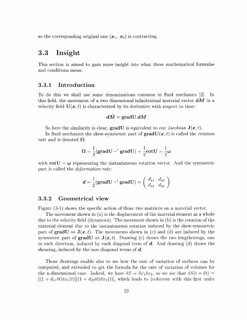
Figure (3-1) shows the specific action of those two matrices on a material vector.The movement shown in (a) is the displacement of the material element as a whole
due to the velocity field (dynamics). The movement shown in (b) is the rotation of thematerial element due to the instantaneous rotation induced by the skew-symmetricpart of gradU M J(x, t). The movements shown in (c) and (d) are induced by thesymmetric part of gradU # J(x, t). Drawing (c) shows the two lengthenings, onein each direction, induced by each diagonal term of d. And drawing (d) shows theshearing, induced by the non diagonal terms of d.
Those drawings enable also to see how the rate of variation of surfaces can becomputed, and extended to get the formula for the rate of variation of volumes forthe n-dimensional case. Indeed, we have 6S =6x1 6x 2 , so we see that 6S(t + 6t) =
[(1 + dtjt)6x1 (t)][(1 + d 2 2 6t)6x 2 (t)], which leads to (coherent with this first order
22
x2 f2
dx2Udt
dxI
(a) X1
x2 t
d22dx2dt\
dlldxldt
(c) X I
wdt/2
(b)
dl2dt
d12dt
(d)
Figure 3-1: General movement of a material element (two dimensions) between t andt + 6t. See text for more detailed explanation.
23
x2 t
X1
XI
x2 f
differential analysis) dS = (d11 + d22)dS. Thus more generally we have
dudivU = Tr(d) = Tr(J(x, t)) (3.8)
dQ
which gives the following result: If the divergence of the velocity field is negative,volumes decrease (known as the Gauss Theorem, a form of transport theorem). Thiscan be refined by saying that: in a region where the trace of the Jacobian is uniformlydefinite negative, volumes that stay in that region, tend to 0. If we consider a system ofdimension n, this means that the state space converges to a space of dimension (n- 1).
We now can understand more intuitively why the skew-symmetric part of theJacobian does not play a role in the evolution of the distance between two neighboringtrajectories: it only corresponds to a rotation of one trajectory with respect to theother, it does not affect the distance between the two trajectories. On the contrary,both the diagonal and non diagonal terms of the symmetric part of the Jacobianplays a role in the evolution of the distance between two points and their respectivetrajectory.
Moreover, a symmetric real matrix is diagonalizable, which means that there ex-ists a base (orthogonal) in which the matrix is diagonal, with its eigenvalues (real)on the diagonal. Thus, if a symmetric matrix is negative definite, it means thatthere exists a base in which its matrix is diagonal, with only negative terms on thediagonal. Hence, in this base, there is no shearing, just negative lengthening on theprincipal directions, so it is clear that distances shrink. Thus, intuitively, two neigh-boring trajectories converges. Indeed, in the general movement shown on figure (3-1),any corner of the square can be viewed as a material point, and as in this case, thesurface of this square is going to 0, whatever couple of corners is representing thetwo neighboring trajectories, they will converge to one another, leading to a singletrajectory.
We can remark here that when the state space is the (x, ±) phase plane, theexistence of a limit cycle implies that the system is not contracting. Indeed, in thephase plane, a trajectory is, at each time, a point. So if the system is contracting,it means that the state of the system will converge to a point in the phase plane(point which is, in general, moving over time). The limit cycle is a space in the phaseplane, in which any point representing a trajectory of the system is going to end upevolving. So it means that each trajectory ends up to follow the same pattern, butspaced by a time interval depending on the initial conditions. So there is an infinityof trajectories. This is for example the case of the van der Pol oscillator.
24
3.3.3 Deeper mathematical explanation
To understand intuitively the change of base/metric reasoning in contraction analysis,we have to remember that a symmetric matrix is associated with an intrinsic quadraticform that has intrinsic eigenvalues. A change of base for a quadratic form, and thusfor a symmetric matrix without changing its eigenvalues, is represented by a unitarymatrix P which verifies P-1 = PT. So a more general change of base, with just aninvertible matrix, like E, applied on a symmetric matrix, does change the quadraticform associated with the matrix, and thus its eigenvalues.
This remark is fundamental to understand the manipulation done in section 3.2.1.In fact, let us consider, to simplify, what happens if E, or equivalently M, is constant(does not depend on time, nor on the state). The generalized Jacobian F = EJ -(as e = 0) is just the matrix of the Jacobian expressed in the new base which isdefined, with respect to the canonical base, by E. Thus the eigenvalues of the gener-alized Jacobian are the same as the Jacobian ones, but here we are interested in theeigenvalues of the symmetric part of the Jacobian, which is a quadratic form, thatis changed in general, as explained, if the change of base is not unitary. Thus themanipulation done in section 3.2.1 indeed changes the eigenvalues of the symmetricpart of the Jacobian, enabling them to become negative as desired if possible.
Another remark is that the sum of the eigenvalues of the Jacobian is equal to thesum of the eigenvalues of its symmetric part (the skew-symmetric part has its sumof eigenvalues equal to zero). Thus the sum of the eigenvalues of the Jacobian in thecanonical base is equal to the sum of the eigenvalues of its symmetric part in any base(as the change of base does not affect the eigenvalues of the Jacobian -the eigenvaluesare intrinsic, associated with the linear transformation that the matrix represents).All these relations are written in the following expression (with A(A) denoting theeigenvalues of the matrix A):
J + JT A(EJ ) A( J- + (JE-1)T
'The trace of a matrix is equal to the sum of its eigenvalues. So, if the trace ofthe Jacobian in the canonical base is positive, there is no way that in another base,defined by a constant change of base matrix E, all the eigenvalues of the symmetricpart of the Jacobian be negative. Thus, the system is not contracting with a constantmetric. Result which can be summed up in the following expression (which provides
'Let us recall at this point that the whole reasoning here applies for the case when E, or equiva-lently M, is constant (does not depend on time, nor on the state). This enables to get some intuitionon the meaning of the mathematical manipulations done. In the case E, or equivalently M, doesdepend on time or the state, these explanations are not exactly true, but one should just feel thatit is a generalization of the constant case.
25
a necessary condition for a system to be contracting with a constant metric):
If Tr(J) > 0, the system is not contracting with a constant metric.
-but might be with a time/state dependent metric-[see footnote of the beginning of theparagraph].
3.4 An example
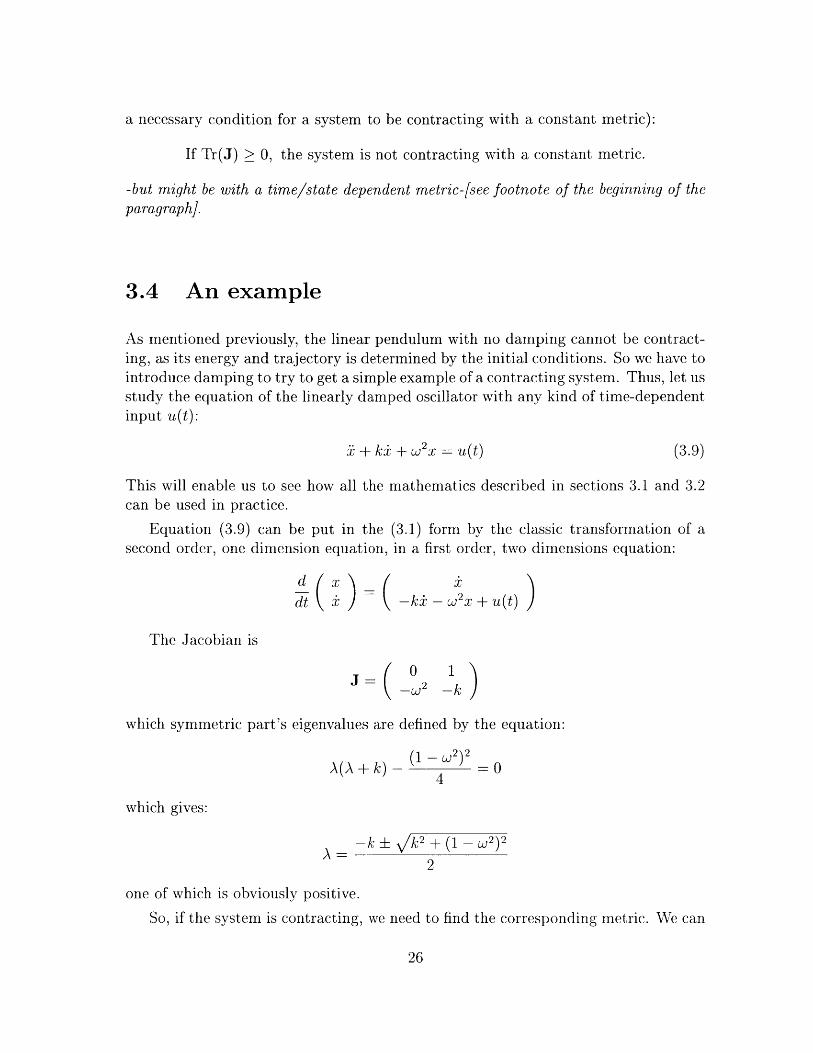
As mentioned previously, the linear pendulum with no damping cannot be contract-ing, as its energy and trajectory is determined by the initial conditions. So we have tointroduce damping to try to get a simple example of a contracting system. Thus, let usstudy the equation of the linearly damped oscillator with any kind of time-dependentinput u(t):
Y + kb + w2 x - u(t) (3.9)
This will enable us to see how all the mathematics described in sections 3.1 and 3.2can be used in practice.
Equation (3.9) can be put in the (3.1) form by the classic transformation of asecond order, one dimension equation, in a first order, two dimensions equation:
d t ) -kz - W2 X + Uft)
The Jacobian is
(02 1
which symmetric part's eigenvalues are defined by the equation:
A(A + k) - (1 - w2 )2 04
which gives:
-k± k 2 + (1- w 2 )2
2
one of which is obviously positive.
So, if the system is contracting, we need to find the corresponding metric. We can
26
try to find a constant metric M=jm b iM12
JTM+MJ= (-10
(the - instead of -1 is there to keep coherent units). Here we know that the matrixM resulting is going to be positive definite, as this is a formulation of the Lyapunovmatrix equation [14], and the system i = J x is stable. Thus we know that M willactually be a metric satisfying the conditions for the system to be contracting.
We obtain, getting rid of a positive multiplicative factor ( ),
(k2 + 2w2)k
k2 )
We now find the matrix
ac
bd
associated with this metric by solving the equation
M = 8ET
which yields to the constant change of base matrix
k/k2 +4w 2
This means that
1-/5 /k 2 +±4w2
As e does not depend on time, O = 0, and the generalized Jacobian equals
F = J-1 =- 12 k2±4 w2
-k vA;2 4 4w2
k2 + 4w2k2 - 4 2
-k/k2±4 w2
27
20 )
We have
kx + 25z/k2 + 4w 2 6x )
( 0/k 2 + 4w 2
2 k
by solving the equation
vI-2
Z -Ivz =
The eigenvalues of the symmetric part are found by solving the equation
(A + k k2 +4w2) 2 - k4 = 0
which yields
A =-k vk2+4w2± k 2 < 0
and thus, the system studied is contracting in the whole state space.Figure (3-2) shows the evolution over time of 6x, and 6z -that is 6x is the new
base. The first one converges to zero, but, as one of the eigenvalues of the symmetricpart of the Jacobian is positive, its norm is lengthening or shrinking depending on theorientation of the (6x, &i) vector. The norm of the second one is always decreasingto zero as the two main directions have a negative lengthening.
0N_0
30
20
10
0
-10
-20
-10 -5 0 5 10 15dx
-20 0 20dz
6 8 10
1200
1000
800
N 600
400
200
00 2 4
time6 8 10
Figure 3-2: Evolution of the distance between two trajectories for the system studiedwith k 1, w- 5. Comparison between the original base (on the left), and the"contracting" base (on the right), for an initial vector (6x, 6±) of (3, 5).
28
5
0_0
-5
-10F
200
150
C'JX 100
50
00 2 4
time
Chapter 4
Mathematical proof of thecontraction behavior of a class ofsystems of interest
4.1 Introduction
As pointed out in chapter 3, contraction behavior can only be found for oscillatorswhich behavior does not depend on the initial conditions. This implies that there mustbe some energy dissipation in a way, and excludes free oscillation like the undampedpendulum for example.
Starting with the equation of the damped oscillator with any kind of time-dependentinput U(t):
+k w k ± = u(t)
which is a contracting system as seen in section 3.4, we felt that adding positivenonlinear terms to the damping should not perturb too much the contracting behaviorof the system. But of course, any nonlinear system needs a precise analysis beforeany conclusion can be drawn.
4.1.1 Statement of the problem
We want to prove that given any function of time u(t), the system verifying
+ (k + ax2)± + w2X = U(t) (4.1)
with w > 0, k > 0, a > 0 and (k, a) y (0, 0), converges to a single trajectory,independent of the initial conditions of the system (but of course dependent on u(t)).
29
Let us call Xo(t) a trajectory of (4.1) -that is a solution of (4.1) given a set ofinitial conditions, and X(t) any other trajectory of (4.1) -that is another solution of(4.1) differing from Xo(t) by the initial conditions. If we define (t) = X(t) - Xo(t)we have:
(o + )+ (k + o(Xo + )2)(Xo + )+ W2(XO + U(t)
or, using the fact that Xo(t) is a solution of equation (4.1),
E + (k + a(Xo + )2)* + (w2 + 2aXoko) + a, g2 = 0 (4.2)
Thus our problem is to prove that limt,+, (t) = 0 for any trajectory Xo(t), thisis for actually any continuous function of time Xo(t) as u(t) can always be defined asu(t) = Xo(t) + (k + aX2(t))Xo(t) +W2Xo(t) so that the function of time Xo(t) chosenis a trajectory of the system.
4.1.2 Intuition
Let us remark at this point that intuitively this result is at least not obvious. Indeedif we look at equation (4.2) and try to interpret it physically, we have:
" the term {(k+ a(Xo+) 2)(}, which is a damping term, depending on time, butalways positive,
" and a spring force term {(w2 +2aXoio) + oaX 2}, which can be interpreted asinduced by a potential of the form {a(t) 2 + b(t)(3}, and thus intuitively couldsuggest that at least with certain initial conditions, is going to diverge (dueto the term in 3).
But trying to find a counter example to the result we wanted to prove failed. Thislead us to the feeling that the dynamic of that potential linked to the dynamic of thedamping was such that, the coefficients {a(Xo + )2}, a, and b, were depending ontime in a way would always be "call back" to 0 soon enough so that it would notdiverge; this is what is proven next. To be more specific, it is interesting to note that
verifying equation (4.2) without the term {(Xo + c)2} in the damping, does notalways converge to 0 in general -there exists some Xo for which does not convergeto 0; thus, in this case, the intuition given by the form of the potential is right. Wecan conclude that the dependence on time of the damping term is fundamental tomake converge.
30
4.2 Demonstration
4.2.1 Integration
Let us rewrite (4.2):
E + k + w2 d + a(Xg + 2XO0 + 2c + 2X 0 ko + -0 02 ) 0
The interesting feature of this formulation is that the term of damping in additionto k is {a(') (X 0 (t)+ K) 2)} which is always positive and thus confines the libertyof Xo(t) in this positive term.
4.2.2 Choice of a convenient origin of time
We will suppose, without restricting the generality of our demonstration, that (0) > 0and define ti as the first time (t) = 0 and (t) < 0, so for t c [0,t 1 , 1(t) > 0.
If t1 does not exist, then limt,+, (t) = 0. Indeed, if this is not the case, as (t)is positive, it would mean that limt,+, j, w2,(()dT = +oc and as the second term of
(4.3) is a constant, and (t)[k+a( +t) +(X 0 (t)+ ))2)] > 0, the only way to counter
it would be that limte+, (t) = -oo which is of course incompatible with the factthat (t) stays positive.
If t1 exists, with the same reasoning, either limt,+) (t) = 0, or there exists a t2such that (t 2 ) = 0, (t 2 ) > 0 and for t E [ti, t 2J, (t) < 0-
31
Let us define h(t) = (t) + (t)[k + c() + (Xo(t) + -i )2)]. We then haveh(ti) = (ti) < 0 and h(t 2 ) = (t 2 ) > 0 thus ]t o E [ti, t2 such that h(to) = 0.
From now on, let us consider that we choose to as the origin of time and rewrite(4.3) for t > to :
+(t) + [(t)[k + a( + (Xo(t) +
4.2.3 Final step
By multiplying equation (4.4) by (t) we get:
M(t) (t) + 2 (t)[k + a( 2 + (Xo(t) +12
and by integrating with respect to time:
2(t)2 + ((r)[k + a( 12 + (Xo(T)
)2)] +
W) 22
W2(()dT = 0 (4.4)
I w2 (T)dT = 0
+(T) )2 + W2 (Td)dT] 2
2 2)]dr+T 22(to)
2
All the terms of the left side of this equation are positive, so if we do not havelimt+O p2 (t) = 0, the term
J t2 (T)[k+$( ) + T)2
12 + (Xo (T) + _) _d
t ok 2 (-)d- or I12 d
goes to infinity and there is no way it can be compensated by another term to getthe whole sum equal to a constant.
It is interesting to note that it is the term corresponding to the damping thatenable us to conclude, which is coherent with the intuition exposed in section 4.1.2.
Thus we have proved that limt,+ $2(t)= 0 and thus that for any input functionof time u(t) the system
, + (k + ax2 )± + ± 2x = u(t)
converges to a single trajectory no matter what the initial conditions of the systemare.
32
4.3 Generalization
Let us generalize this result and prove it for the systems verifying:
z + (k + ax2 ")d + wx = u(t)
n being an integer.It is already true for n = 0 and 1. Let us prove it for n = 2.The only thing we have to do in order to be able to use the previous demonstration
is to put the equation that satisfies in the form of (4.3) where the important featureis that the term in addition of k in the damping is positive.
At this point we would like to prove that the expression E"O 2n-X 2nk is
34
or
always positive.
Let us manipulate this expression in order to prove what we want:
1 2n
1 ZC n+1X 2 n-k -
k=O
(Xo + 2n+1 _ X 2n+l
(2n +1)
2n+1 0
Of course in the two last expressions we have to exclude the times when X 0 (t) = 0or (t) = 0, which is fine as at those times the expression we are looking at is 0 andthus positive.
Now, excluding those cases, the sign of this expression is given by the sign of{{[(1 +I )2n+1 _ 1]}
" either X 0 and have the same sign and the two factors of this expression arepositive, so is the expression.
" or X 0 and have an opposite sign and the two factor of the expression arenegative, and the expression is positive (as either {1 > 1+ > 0} and {(1 +
)2n+ - 1 < 0}, or {1 + < 0} and the second factor is also negative).
This is the result we were looking for and by defining
2n k
w(e (t) (t)) = w 2n X2n-kk=O n k lO
we can write
S+ k +w2 [dd [cal(Xo t), (t))] 0
which integrates in
(tW 2 (T)dT -- (0) + (0)[k + a (X(0), (0))]
and as {ca(X 0 (t), (t)) > 0} the same reasoning as in the case n = 1 holds whichleads us to the following general result:
The system verifying
z + (k + ox 2,). + w = u(t) (4.6)
35
k=On - Xk 2 nk
(4.5)
) 2n+1X0
(()+ (t) [k + wl (X0 (t),()) +
(n being an integer; w, k, and a positive real numbers with (k, a) # (0, 0)) convergesto a single trajectory -depending of course on all the parameters n, W, k, a, and u(t),but not on the initial conditions.
4.4 Extension
4.4.1 Result
The last result can be generalized to get the following result:Given P(x) = EN- /X 2 n with Vn /n > 0 and not all the #3 equal 0,
i + [P(x)] + w2x = u(t)
converges to a single trajectory in the same sense as described before.
4.4.2 Proof
Indeed, everything works the same way:We have:
the system
(4.7)
(X0 + ) + [P(X 0 + ( + + W2 (Xo + ) U(t)
which gives us
N 2n-1
+ w2 +v + ( 3E X 0 ( Z C4 Xk 2 n-k) +n=1 k=O
2n
2 +k=1
C2 Xk 2 n-k)l = 0
2n
O (Sn=O kr=O
CkC2 " Xk2n2n - k +1
which, by defining D2n (XO(t), (t)) = 2n C2_ X 2n-k > 0, we can integrate in
The fact that ENO On 42n(Xo(t), (t)) > 0 enables us to follow the same reasoningas in sections 4.2.2 and 4.2.3 which leads us to the result stated in section 4.4.1.
36
+ w 2- +[
dtk)] = 0
4.4.3 Simulation
Figure (4-1) shows an example of such a behavior for the system:
, + k(3X 2 + 3x 8 ) + w 2x = ln(1 + sin 2 (t))
with k =1, w = 1, and the initial conditions for the two systems: (Xi(0), ±l(0), X2 (0), 2(0))
(2, 1, 1, 0). This example was chosen so that it would not be simple, and thus give aninteresting illustration.
50 100 150 2Ctime
0.5 -0
0
-0.5'0
0.4
0.2
0-a. 0
-0.2
-0.450 100 150 2(
time
0
_0V~X
0 50 100 150 200time
50 100 150 200time
0 50 100 150 200time
0.5 F
0
-0.5'0 50 100 150 200
time
Figure 4-1: Contracting behavior of , + k(3x 2 + 3x 8 )± - w 2x = ln(1 + sin 2 (t)) withk = 1, i = 1, and (xi(0), Ji1(0), X2(0), x 2 (0)) = (2,1, 1, 0).
4.5 Higher order
We can extend this result to the study of higher order systems of the kind
±(n+2) + [P(x)]x(n+ 1 + W2(n (t).
Indeed, the result we get applies to x('), and thus we know that for any initial
37
X
3
2
1
00
1
1 0.5
0C
2
1
0
-1
-N
OMM -
. . .
-0
0
1
-- 4
conditions of the 0 to (n + 1) derivatives, the (n), and higher order derivatives, willconverge to a single trajectory. Or in another way, (n), (n+1) and (n+2) will convergeto 0, and thus (n-1) converges to a constant, (n-2) is converging to a linear function,and so on, so that we at least know how the two neighboring trajectories diverge(which is determined by the way behaves).
38
Chapter 5
Studies of Contraction of systems
requiring the use of a Metric
5.1 Contraction analysis of a class of system simi-lar to chapter 4's
The generalizations made in the previous chapter lead us to wonder what is thesituation for a similar kind of class of systems. Thus, let us look at the systems ofthe form
+ + k± + w2Q(x) = u(t) (5.1)
with Q(x) = 0 Yn 2 n+ 1 with Vn ps., > 0 and not all the p, equal 0.
5.1.1 Introduction
The intuition is that we are adding to the linear damped oscillator only potentials ofthe form nX2n+
2 which are stabilizing.
Moreover, trying to derive the same kind of proof as in the previous chapter startswell. Indeed we have, with the same notations as previously,
(X 0 +) + k(Xo +) +w 2Q(Xo-i+) = u(t)
which gives us
N
W2 k w 2 pn[ (Xo + )2n+1 _ X2n+l] = 0n=O
39
or
. . U)2 N (XO + )2n+1 - X2n+1& + k g + 2 6 Z' pn[ -]X= 0 (5.2)
n=0
Now we know that the expression in brackets is positive, as it is the one studied inderivation (4.5) times (2n+ 1). Equation (5.2) is very similar to the damped oscillatorone with no input; a time-dependent factor is modifying the last term but is alwayspositive. Thus we could legitimaly think that it would behave the same way thedamped oscillator does, and that we would be able to prove that limt,+oo (t) = 0.So we tried to use the same kind of proof than the one exposed in section (4.2), takingadvantage of the fact again that the indefinite function of time Xo(t) is confined ina positive term. Unfortunately, although the first integration works out well, as wellas the argument about the convenient origin of time, the second integration carriedin the final step cannot be done.
At this point, although we felt we were close to the result, we could not get itrigorously, and some simulations showed us why: in general this type of system isnot always contracting. Indeed there are some counter examples. For example thesystem z + 0.1± + x5 = 6 sin(t) with initial conditions (2, 3) is chaotic, figure (5-1)shows the simulation. 1
But some other systems of this type are definitely contracting; finding a conditionfor a system of this type to be contracting is thus of interest.
We now can notice that the fact that in general the system (5.1) is not contract-ing can be understood by remarking that, contrary to the linearly damped oscillator,here, in equation (5.2), the force that is applied to depends on the trajectory Xo(t),and thus has no reason to converge to 0 in the general case - which makes the resultsfound in chapter 4 even more interesting.
We apply Contraction Analysis using a time varying metric to find a condition onthe system to be contracting. In the general case, trying to find a time varying metricis difficult as there is no general method for that. Here, as the system has the sameform of equation as the damped oscillator's, we tried to find a time varying metricclose to the constant one found in section (3.4). This method works out well becauseof the particular form of the Jacobian, featuring the same kind of property as the oneof the damped oscillator. The type of systems studied in chapter 4 contains a productof type x., which appears in the Jacobian, and consequently make the direct searchof a metric intractable. This is why we were lead to a different derivation than theone conducted here; but we will come back in this chapter on the contraction analysisof the system (4.1) to be able to prove the exponential property of the convergence
'Chaos can only appear with at least third order systems when there is no input. Here the systemis second order, but there is a driving force which self frequency has nothing to do with the one ofthe system, which is a supplementary source of disorder and thus induces the chaotic behavior.
with R(x) = dQ(x) = nZ$2i0 (2n + thus R(x) > 0 which is fundamental tobe able to choose for this case the following extension of the metric M of the lineardamped pendulum as
[k 2 + 2w2R(x)]k
k2
which is thus definite positive.We now find the matrix
aC
bdJ
associated with this metric by solving the equation
M = OETE
which yields
12 k2 + 4w2R(x)
and
0v-2w 2 R'(x)
Vk 2 +4w 2R(x)
0
0
k+ 4w2R(x)
(
)
20 )
0Vk 2 4w 2R(x)
dwith R'(x) =dl
2 k-k J
R(x)
This yields the generalized Jacobian F = (63 + 0J)8-
1F 2 j + 4W2R(x) -k k2 + 4w 2 R(x)k2 + 4w2R(x)
k2 - 4W2 R(x)
4w2R(x)- k jk 2 + 4w2 R(xc)k24w2 R(x)
42
)
The condition for the system to be contracting is that the generalized Jacobian benegative definite, which is equivalent to the following matrix being negative definite:
The eigenvalue computation gives the following two conditions2
k(k 2 + 4w2R(x)) - 2w 2 R'(x) > 0 (5.3)
and
k(k 2 + 4w 2R(x)) - 4w 2 R'(x) > k3 (5.4)
The first condition leads to: 0 +2kR(x) > R'(x) and the second to: kR(x) > R'(x).Thus, as R(x) > 0, if the second condition is verified, the first one is automatically,and we obtain the condition for the system to be contracting:
kR(x) > R'(x) (5.5)
5.1.3 Interpretation
So basically, this is always true if R'(x) < 0; and if k is large, there is less restriction onthe trajectory, which is verified in simulations. This is of course a sufficient conditiononly.
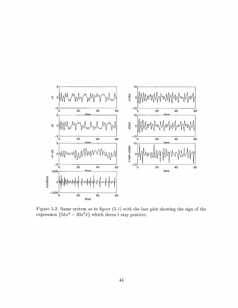
It is satisfying to remark that this condition is not verified for the chaotic counter-example shown in figure (5-1). This case is reproduced on figure (5-2) with the lastplot showing the sign of the expression supposed to be positive (and which is not).
A simple example of this condition being satisfied appears when a trajectory ofthe form x(t) = a + be-" (with a, b, c > 0) is picked, for which R'(x) is always goingto be negative as R'(x) = n0 2n(2n + 1)pnx 24 1 ± and x > 0 and ± < 0. Such anexample is shown in figure (5-3).
Given this condition, and a particular system (giving k and R(x)), we can plot thecontraction region in the phase plane (x, -) in which the trajectory has to stay to guar-antee contraction. Figure (5-4) shows this region for the system: , + 10 +1 Ox + x5
U(t).
If we know that R(x) is never going to be null (for example if the x coefficient in
2 We get aA2 + bA + c = 0 with a = 1, b = 2k(k 2 + 4W2 R(x)) - 4W2 R'(x), and c = k(k 2 +4w 2 R(x))(k(k 2 +4W 2 R(x)) - 4W2 R'(x) - k3 ). We have A = -b±2 b-4ac The conditions correspond2arespectively to b > 0 and c > 0. As the matrix is symmetric real we know that its eigenvalues arereal and thus that the determinant A = b2 - 4ac is positive.
43
10
0
60
10 tm
0c\j
-100 20 40 60
10 -timia
- 0.0
-10 -
0 20 40 60time
Figure 5-2: Same system as in figure (5-1) with the last plot showing the sign of theexpression {5kx 4 - 20x 3±} which doesn't stay positive.
44
5
0
C\ 0 2
5 im
0 20 40
5 ime
c'j
60
60
60-5
1 OC0 20 40
C
~00U
0
- IUU0 20 40
time60
0 20 40
20 40
0 20 40
4
.; 3.5 -
3 '0 2 4
5 ,
4X
3
20 2 4
0.2
0X
6 8 1M'
6 8 1imP
0
3 -0.5-x
0
0
X
05-0N~XI5
0
X
0 4 2 4 6 8 101 xl, time ,10
0
-5-
00 2 4 6 8 10
time
-1 -
020I
0
-20 020!
0
-200
2 4 6 8 10
2 4 6 8 10tim
2 4 6 8 10time
Figure 5-3: Contraction behavior of the system ,++x 3 +x 7 e-t -e-t+(3+et-)3 +(3 + e-) 7 and initial conditions (xi(0), zI(0), x 2 (0), ±2(0)) (4, - 1, 4.1, - 1.1).The last plot shows that the expression {kR(x) - R'(x)} is always positive and thusthat the sufficient condition for the system to be contracting is satisfied -and we cansee that the system is indeed contracting.
45
' ' ' ' '-0.2
80
60
40
20
0_0x 0
-20
-40
-60
-80-1 -8 -6 -4 -2 0 2 4 6 8 10
x
Figure 5-4: System ± + 10± + 10x + x5 = u(t). The contraction region lies betweenthe two plotted curves.
46
................. ..............
- .
- ...
-. ....-. ....-. .-.- .
- .... .. .... .... ...... ...
-. . .. ... .. .
... ...................... ... ... -
............... ........ -
. .- -.. .-.
0-
Q(x) is not null, that is [o # 0), this condition can be rewritten as:
k>R'(x)dk > ='(x - d[ln(R[x(t)])]R(x) dt
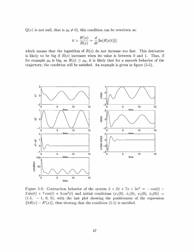
which means that the logarithm of R(x) do not increase too fast. This derivativeis likely to be big if R(x) increases when its value is between 0 and 1. Thus, iffor example [to is big, as R(x) ;> po, it is likely that for a smooth behavior of thetrajectory, the condition will be satisfied. An example is given in figure (5-5).
2
-20 5 10 15
1 , time
-1C\ 0
0 5 10 152 timin
C\1X
0
0 5 10 15100 timo
5 50-50
00 5 10 15
time
0-0X -1 -
0 5 10 152
0-
-2
0 5 10 152 time
~0~-
0
-40 5 10 15
time
Figure 5-5: Contraction behavior of the system ,% + 2i + 7x + 3x 3 = - cos(t) -2sin(t) + 7cos(t) + 3cos 3 (t) and initial conditions (xi(0), ±I(0), x 2 (0), ±2(0))(1.5, - 1, 0, 0), with the last plot showing the positiveness of the expression{kR(x) - R'(x)}, thus showing that the condition (5.5) is satisfied.
47
5.2 Scalar system
5.2.1 Introduction
One question which occurs naturally when studying contraction theory is: Is a systemexponentially convergent with a 0 input, contracting ?
Let us study the case of the following scalar system:
S=-g(x, t) x + u(t) with V x, V t, g(x, t) ;> a > 0 (5.6)
If u(t) = 0 (nominal system), this system is exponentially converging as we have
± d- ln(x) = -g(x, t) < -a -> x(t) < xoetx dt
Contraction theory studies the behavior of the infinitesimal distance 116xl| betweentwo neighboring trajectories, which has no reason to converge exponentially (oneshould always have in mind that contraction analysis is valid for any input u(t)).Indeed the Jacobian of the system is
J(x, t) - -g(x, t) - x g(X, t)
ax
which has no reason to be always negative.
For example if g(x, t) = 1 + (x - 5)2, the Jacobian is J(x, t) -1 - (x - 5)22x(x -5). If we take X(t) -3+ 2 arctan(t), choose u(t) X(t)+g(X(t), t) X(t) andset the initial condition to the adequate value X(0) = 3, then X(t) is the solution ofthe differential equation (5.6), thus X(t) is the trajectory followed by the system. Inthis case, the system is starting at 3 and increasing tending to 4, and the Jacobian isalways strictly positive, starting at 7, increasing, and then decreasing tending to 6.
If the Jacobian is always negative, the system is contracting in the whole statespace. This is the case for example if g does not depend on the trajectory, whichimplies that L9 0 and J(t) = -g(t) < -a < 0. Or also if g(x, t) is increasing withax
x for x > 0, and decreasing with x for x < 0.
For the case the Jacobian is not always negative, determining whether the systemis or is not contracting implies to find a metric.
48
5.2.2 Metric search
As exposed in sections 3.2.1 and 3.2.2, if a metric m(x, t) uniformly definite positiveexists, there must exist a # > 0 such that
In the regions where J(x, t) < 0, any positive constant is a metric. In the regionswhere J(x, t) > 0 we see that the metric has to be time dependent so that the in-equality (5.7) can be verified.
Now if the Jacobian is always positive we have
Th(X, t) < -#m(X, t) -> m(X(t), t) < m(XO, 0)e-,3
and thus there is no way we can find a metric uniformly definite positive, and thusthe system is not contracting (converse theorem -section 3.2.2).
Here we can remark that this result can be derived just by looking at the equation-_ J(x, t) 6x. Indeed, this equation means that, anytime the distance between two
neighboring trajectories is infinitesimal, its dynamic verify this equation. And thusif J(x, t) > 0, such an infinitesimal distance always stays constant or increase, so itcannot converge to 0. So the system cannot be contracting.
In the case when the Jacobian changes sign over time we obtain a necessary andsufficient condition for the system to be contracting by the following: we have fromequation (5.7), as m(x, t) > 0,
rh~~, t)= n (m (x, t)) < ( + 2 J(x, t))m(x, t) dt
-> (x (t),7t) < mn(x0) C-- fA ( +2J x T, ))d
thus
a necessary and sufficient condition that a uniformly positive met-ric m(x(t), t) exists is that there exists a # > 0 such that the integral
0'(#+ 2J(x(T), r))dT be upper bounded over time.
Indeed if this is not the case, this integral tends to infinity, and m(x(t), t) cannotbe uniformly positive.
49
And if it is the case, we have
3 # > 0 and " A > 0 such that V t j(3 + 2J(x(T), T))d < A (5.8)
is uniformly definite positive (with of course m(xo, 0) chosen to be strictly positive).The condition (5.8) is equivalent to
El >0and 3 A >0 suchthatV t J(X(r), 7)d7 < A2
which means that the Jacobian in mean is enough negative over time, even though itmight be positive sometimes; the condition is that the integral of the Jacobian overtime tends to -oc at least linearly with t.
5.2.3 Example
An example of condition (5.8) being verified although the Jacobian gets positive aninfinite number of times as t goes to infinity is the following:
We take g(x, t) = (x + 5)2 + 1, and make the trajectory be X(t) = sin(t) - 5 (bychoosing u(t) = cos(t) + (sin(t) - 5)(sin 2 (t) + 1) and X(0) = -5).
The Jacobian is in this case J(x, t) = -(x + 5)2 - 1 - 2x(x + 5), which is for thistrajectory, J(X, t) = -3 sin 2 (t) - 1 + 10 sin(t), and thus is not always negative as forexample t =[2ir] - J 6.
Let us look now at the integral of the Jacobian over time:
(m(X(0), 0) being any strictly positive number). O(X(t), t) which verify 02 (X(t), t)m(X(t), t) is such that 6z = 0(X(t), t) 6x is always decreasing.
50
Figure (5-6) shows the simulation.
-a
C
1ic
0
10
5time
10
0 5 10 1time
-20 '-0 5
time10
x
-3
-4
-5
-6
-715 ) 5 10 1
time
N-a
0
-15 0 5
time10
15
Figure 5-6: The two plots on the first line show: on the left, the nominal trajectory, onthe right, the perturbed trajectory (with initial perturbation equal to 0.01). The firstplot of the second line shows the difference between the nominal and the perturbedtrajectory (which tends to 0 as the system is contracting). The second plot of thesecond line shows 6z = O(X(t), t) 6x which is always decreasing as the GeneralizedJacobian F + J is negative definite (~ -2.5). And the last plot shows theJacobian over time, which is not always negative, still the system is contracting withrespect to the metric m(X(t), t) (here m(X(0), 0) = 4.104).
51
-4 -
X -5
-6 -
-70 5
15
00
-
2
1.5r1
1
O.5
1
5.3 Study of convergence of the state space of an dimensional system to a space of dimension
(n - 1)
5.3.1 Introduction
The following second order system
Sz=y + X(1 -X2 _ 2)
-X + y( - X2 _ Y2)
with initial conditions different from (0, 0), tends to a limit cycle [10]. This canbe shown with the Lyapunov function V(x, y) = (1 - x2 _ y2 )2 which is such thatV(x, y) = -4(X2 + y2)V(x, y), and thus the system tends to the centered circle ofradius 1. So this second order system tends to a one dimensional system.
Let us study this property using the result stated in section (3.3.2): in a regionwhere the trace of the Jacobian of a system is uniformly definite negative, volumes ofthis system which stay in this region, tend to 0. If we consider a second order system,this means that the state space in this region converges to a one dimensional space.An interesting feature of this result is that, like the Contraction property, it does notdepend on any time varying input added to the system. Thus we are looking at theproperty of converging to a one dimensional space for the following system:
Sy + X(1 - X2 _ Y 2))ut
( )X + y(I x2_ 2) ) ± V (t)
5.3.2 Second order system
The Jacobian of this system is
J 1 - 3X2 _2 1 -2XY-1 - 2xy I - x2 - 3y2
and we get Tr(J) = 2 - 4(x 2 + y2 ). This trace is thus uniformly definite negative inany region of the two dimensional state space excluding strictly the centered circle ofradius 1 . And thus the state space in {!R2/C(0, )}, the exclusion being strict, isconverging to a one dimensional space. This means that all the trajectories stayingin this region converge to a one dimensional space -this space being time dependentin general.
We can extend this restriction on the trajectory by trying to find a change of baseE in which the trace of the generalized Jacobian F is still uniformly definite negativealthough the trace of the Jacobian itself (in the canonical base) is not. Indeed, in a
52
region where Tr(F) is uniformly definite negative, volumes converges to 0 too, as thisproperty does not depend on the base in which volumes are computed, the same waythe dimension of a space does not depend on its base.
We have F = 00-1+J0 which implies that Tr(F) = Tr(60-1 )+Tr(OJO01 )Tr(00') + Tr(J). Tr(F) is uniformly definite negative within a certain region isequivalent to
3 E > 0 such that V(x, y) in that region Tr(F) < -E
or, taking into account the expression of Tr(F) derived,
3 E > 0 such that V(x, y) in that region Tr(60- 1 ) < -E + 4(x2 + y2 ) - 2 (5.9)
Now, for any change of base matrix O(t) = (t) b(t) we have det(0)c (t) d (t) ]
ad - bc, which has to stay uniformly different from 0 so that the associated metricM = )T 0 is uniformly definite positive. We have, by computation
Tr (6 -1) - det (0)det(0)
Combining with equation (5.9) we get
det ()< -E + 4(X2 + y2 ) - 2det(0) -
which gives
Sdet (E)(t))| < Idet (E)(0)) 1 eCfO'[-+4(X2(T+y2(T))-]d
Thus f[-E + 4(X2(T) + y 2 (T)) - 2]dT has to be lower bounded so that det(0) canstay uniformly different from 0.
Thus we have the following necessary and sufficient condition for the trace of F
to be uniformly definite negative:
E E > 0 and 3 B < 0 such that V t [4(X2(T) + y 2 (T)) - 2]dT > B + Et (5.10)
which intuitively means that the trajectory does not enter too much over time the
centered circle of radius .
If this condition is verified, we can choose any matrix 0(t) such that det(0(t))det( (0)) efKE+4 >(T)y(T)>-2]dT (with det(6(0)) being any strictly positive num-
det((0))efj[-e4(x2 (T)+y 2 (T)>2]dT 0 '
ber), for example 0(t) = det(E(0)) 0 1 , and the trace of
53
the generalized Jacobian associated with this change of base is uniformly definite neg-ative. Thus, all the trajectories within the region verifying condition (5.10) convergeto a one dimensional space (in general depending on time).
See last paragraph of next subsection for a discussion on why starting this wholereasoning at t = 0 (as it is done here), or at any other time t = to leads to the sameresult on the dimension of the space to which the trajectories converge, with the samenecessary and sufficient condition.
5.3.3 n dimensional case
It is interesting to note that the relation
Tr(eO1 - det ( ) (5.11)det(0)
is true for any dimension. Indeed we have the following equality, true for any invertiblematrix,
1 _ 'Com(E)det(0)
Com(e) being the matrix composed of O's cofactors. We then see by computation3
that Tr(e Com(e)) = det (e), which leads to equation (5.11).We thus can extend the previous result to any system of any dimension.
Let us consider a n dimensional system of the form + = f(x, t). We have, asexplained previously, Tr(F) = Tr(60-1)+Tr(J). Tr(F) is uniformly definite negativeis equivalent to
] E > 0 such that Vx Tr(F) < -E
or, using the previous derivations,
A E> 0 such that Vx det (0) < -E- Tr(J(x, t))det(0)
which leads similarly to
I det (E (t))l < I det(E)(0))l cf1E -'_' (X(T)'T))]d-
3 or by differential calculus: considering the analytical properties of the determinant, we haved(det(E)).6 = Tr(OtCom(E))
54
and thus, J [E + Tr(J(X(T), T))]dT has to be upper bounded so that det(9) can stayuniformly different from 0.
Thus we have the following necessary and sufficient condition for the existence ofa generalized Jacobian F which trace is uniformly definite negative:
SE >0 and ] A> 0 such thatVt j Tr(J(x(T), T))dT < A - Et (5.12)
and if this condition is verified within a certain region, all the trajectories within thisregion converge to a space of dimension (n - 1).
Let us note that, to conclude that all the trajectories within a region convergeto a space of dimension (n - 1), only the behavior when t tends to infinity matters.Indeed, if trace of F is not uniformly negative from t = 0, but only from any fixedtime t = to, the same reasoning apply. Indeed, it means that the rate of variation ofvolume may not be always negative for t C [0, to], but as this interval is bounded, weknow that volumes at t = to will be bounded, and thus volumes will still converge to0 as t goes to infinity if the trace of F is uniformly negative for t > to.
And actually, the necessary and sufficient condition (5.12) found, does not dependneither on the origin of time. Indeed, if to exists such that
3 E>0 and AO > 0 such that Vt> to ] Tr(J(x(T), T))dT < Ao - Et
then
3 E > 0 and ] A > 0 such that V t Tr(J((T), T))dT <A - Et
/tas A can for example be defined by A = Ao + f4o Tr(J(X(T), T))dT. This actuallyshows that if a matrix 90 exists such that the trace of the corresponding generalizedJacobian Fo is uniformly definite negative for t > to, then there exists a matrix 0such that the trace of the corresponding generalized Jacobian F is uniformly negativedefinite for all t.
5.4 Study of exponential convergence for the sys-tem introduced in 4.1.1
5.4.1 Introduction
Inspired by the studies of contracting regions for different types of systems in thebeginning of this chapter, we try here to determine a region where the system intro-
55
duced in 4.1.1 is contracting. This would enable to have the exponential convergencein this region, and thus a stronger result, for this region, than the one we get inchapter 4. Indeed, the result proved in chapter 4 is valid for the whole state space,but does not prove exponential convergence -still, by looking at the similarities be-tween the equations and the linearly damped oscillator equation, such an exponentialconvergence is very likely.
5.4.2 Analytical Study
We use the constant metric found when studying Contraction for the linearly dampedoscillator (section 3.4). We compute the generalized Jacobian, and the required neg-ative definiteness of the generalized Jacobian imposes a condition that defines thecontracting region with this metric.
The system is
i + (k + ax2 )± + w2x - u(t)
Its Jacobian (with the variables (x, ±)) is
.- x _- W2 (k + ax 2 )
The change of base e corresponding to the constant metric found in section 3.4 is
1 k 2/ ( k2-+4w
2 0
and we have
0 2/2/k2 4 w2 ( k2 ± 4w 2 -k
As 9 does not depend on time, O = 0, and the generalized Jacobian equals
The solutions of the corresponding second degree equation in : are
1 k(x + ) -I k (k2 ± 4W2)( + 2a) (5.14)4 [ ax a x2
As 16a 2X2 > 0, the inequality (5.13) is true if ± lies between the solutions (5.14).This defines a region in the (x, ±) plane in which the system is contracting. As(5.14) is not defined for x = 0, this region is actually defined by 4 asymptotic curves,symmetric 2 by 2 with respect to the origin.
5.4.3 Visualization and interest
Plotting these curves for different values of k, a, and w enables to visualize whatthis region looks like. It then enables to realize that it can contain (depending on thek, a, and w coefficients) the limit cycle of the corresponding van der Pol oscillatordefined by
+ a(X 2 - 1)w+ 2 x = 0
with the same coefficients a and w.
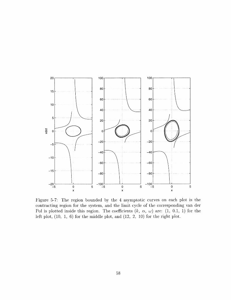
Plots showing the region, and the limit cycle of the corresponding van der Poloscillator, for different sets of coefficients, are presented in figure (5-7).
The interest here, is that we thus know, that if the trajectory followed by thecontracting system is the one of the corresponding van der Pol, this trajectory iscontracting.
57
20 1
151-
10
5
0
-5
-10
-15
-205 0
100
80
60
40
20
0
-20
-40
-60
-80
-100-5 0 5
100
80
60
40
201
0
-20
-.
- - - - --.
-- -- - -- --.
-. .. .... . . ..
-r
- .--....- ... -. .
Figure 5-7: The region bounded by the 4 asymptotic curves on each plot is thecontracting region for the system, and the limit cycle of the corresponding van derPol is plotted inside this region. The coefficients (k, oz, w) are: (1, 0.1, 1) for theleft plot, (10, 1, 6) for the middle plot, and (12, 2, 10) for the right plot.
58
0
-40 -
-60 -
-80--
-100-5 0 5
x
-......... -.. ............-
- -
-....
-
-1
5.5 Contraction study of the damped van der Polusing a change of variables
5.5.1 Introduction
The damped van der Pol is the original type of system studied in chapter 4. Wethere show that this system has a contracting behavior as it converges to a singletrajectory. Section 5.4 studies cases when this convergence can be proved to beexponential using Contraction Theory with the canonic variables (x, i). Here, usinga change of variables, we are able to refine this result using again Contraction Theory.
5.5.2 Change of variables
We are studying the following previously introduced system:
+ + (k + aX2)± + w2x = u(t) (5.15)
When studying van der Pol oscillators of the form z + a(x2 - 1)± + w2 x = 0, auseful change of variable is (x, ±) 4 (v, w) with v = x, and w -x + _ + y,
i) = (W - V + Vwhich leads to {ba w W . This formulation of the equations creates two
distinct variables whose dynamics act in different time domains for a / 0(1). Forexample for a > 1, v can be seen as the fast variable, whereas the changes in w occuron a time scale that is ' slower than for v. This is useful for large or small values ofa as it allows to treat the variables separately, thus considering for example the slowvariable as constant with respect to the fast transitions.
Inspired by this "slow/fast" change of variables, let us introduce the followingchange of variables for our system:
k x 3 ±x = (x, ) = x=(x, y) with y = -X + + -
a 3 a
The system (5.15) is equivalent to the following system in (x, y)
{ * (y - X - k)W2X+
59
So if the system
(5.16)
is contracting -that is, whatever time dependent input is added to the system (5.16),the system converges exponentially to a single trajectory- then a fortiori, the system(5.15) is contracting.
5.5.3 Contraction study
The Jacobian of the system (5.16) is
-a(x2 + k)
W2
ae
_1a
Sa2(X2 + k)W2
The two eigenvalues of the symmetric part of J in this base (the canonic base) arealways of opposite sign, so to study contraction, we need to find a metric.
Let us introduce a general constant E matrix linked to the corresponding metricM by M = ET
ac
bd and we can writeI )
ad-bc (d
-c
-b
The generalized Jacobian F then equals
F = OJE-1a(ad -bc)
aC
b)(d )
Z2(x 2 + k)
-iw2
a 2
0 )( d-c
-ba )
which gives us
1a(ad -bc) (-(ad a 2 (x 2 + k) + bd w2 + ac a 2)
-(dc a 2 (x 2 + Z)+ d2 W2 + c2 a2)
ab a 2 (x 2 + )bc a 2 (x 2 + -)
+ b 2 2 + a2 a2
+ bd w2 + ac a2
which, to simplify the formulae, we write as
F _1 (F a -IF a (ad -bc) \-fi
- f21f12
f 22)
We want the symmetric part of this matrix to have its two eigenvalues always
strictly negative. This is true if ad - bc > 0 and if - 2fii( fi2 - f21
fl2 - f212f22 )has its
two eigenvalues always strictly negative. The second condition is equivalent to thesecond order equation (A+2f, )(A -2f 22 )-(f 12 -f 21 )2 2+2(f, -f22)A-4fn/22
60
a 2
0 )
)
a(Y X3 k3 X)
_W2XY a
(f12 - f21) 2 = 0 have its two roots always strictly negative. Thus we need to havefli - f22 > 0 and -4f11f22 - (f12 - f21) 2 > 0. The first inequality is equivalent to(ad - bc)a 2 (2 + ±)> 0 - ad - bc > 0.
So we end up with the two following condition for the system to be contracting:
{ ad - bc> 0
4f11f22 + (f12 - f21) 2 < 0
The second condition leads, after a certain amount of computation and manipu-lation, to the following second order inequality in the variable (x2 + k)
which implies (as a 4 (ab + cd) 2 > 0) that the value of (X 2 + k) has to be between theroots of the second order equation.
The constant term of this second order equation is positive as it is also equal to4(bd w2 +ac G 2 ) 2 + ((b2 - d2 ) 2 +(a 2 - c 2)a 2) 2. Thus the two roots of this equation areof the sign of -2a 2 (ab+cd)[(b2 +d 2 )W 2 + (a2 +c 2 )a2], that is of the sign of -(ab+cd).Thus, if we want the preceding second order inequality to have a possible solution,as (2 + I) > 0, we need to have -(ab + cd) > 0.
Again after some computations, that simplify well though, we obtain the two rootsof this second order equation:
Thus the contracting region is defined by 2 satisfying the following double in-equality:
k (b2 + d2 )W2 + (a2 + c 2 )a 2 2w |ad - bc| 2
a a2(ab + cd) a |ab+ cd|
k (b2 + d 2 )W2 + (a2 + c2 )a 2 2w |ad - bcja a2 (ab+ cd) a lab+cd|
To determine how to have this contraction region as large as we want, let us seta positive real A as big as we want, and define the contraction region desired by{x such that x2 < A}.
Thus we want the left hand term of the last double inequality to be negative orzero, and the right hand term to be bigger than A.
61
One way of achieving this is to define (a, b, c, d) and k such that they satisfy
4w |ad - bc| k= A and
a |ab+ cd| a
(b2 + d2 )w 2 + (a 2 + c2 )a 2
a2(ab + cd)
2w |ad - bc|c lab+ cd|
-the condition ad - bc > 0 has to be satisfied too.
We then obtain that the contraction region is the one desired, as it is defined by0 < x 2 < A. (4)
Let us give an example of simple values of (a, b, c, d) and k that satisfy all theconditions desired:
First let us set b = 0,c = -, and a = A which implies, if d >4w Iad-bcl A, ad-bc = id > 0, and ab+cd= -wd < 0.a Iab+cdl 4
0, that
We now need _ k _ (b2 +d 2 )w 2 +(a 2 +c 2 )0 2
a a2(ab+cd)
which leads to k = a (dg + ( + w) - (9. The function f (d) =
for d E R+ is first decreasing then increasing, its minimum value being 2 + a.
Thus the value of ; determines the minimum value that k can take, which is
k = a(2 ( + - ford a2(1 + ). k can then take any value su-
perior to its minimum by determining the matching d.
Thus for any B fixed and any region defined as IxI < B, we can find a metric
in which the system (5.15) is contracting for any k > a (2
B 20
metric is M = ETE with (= 4-t k
value is linked to the value of k.
J34 w2 B2\16 C 2 2 This
0 ), d being any strictly positive number, itsd
This result refines the one obtained in the previous section: the system convergesexponentially to a single trajectory in any bounded region, provided that k is superiorto a certain minimum value. It is interesting to note that this minimum value doesnot diverge as B goes to infinity -and is even minimum for B tending to infinity.
4-Of course, more precisely we want 0 < x 2 < A, which can just be achieved by taking k slightlybigger than the value defined here.
62
_ 2ad-cl -+ d2W
2 +( A2 ++2
a ab+cdl a a2 (wd) A = 02
5.6 Weak Contraction study of the damped vander Pol
5.6.1 Introduction
The result of the previous section, which leads to a minimum value of k which isminimum for B tending to infinity, made us feel that a more general result could bederived.
B32a
We first remarked that for large B, we had d ~ 4B and E~ 4 22 -4w
4 ( 1, which suggested that taking 2y instead of y as the second variable\ B2 s tk
would simplify the calculus. It actually does simplify a little the formulae, but doesnot change the reasoning and the different stages of the calculus. We obtain the sameresult with the same condition on k.
But, at the beginning of the calculus one interesting thing appears: With this newsecond variable, the Jacobian in the canonic base is semi-contracting, and thus wecan carry the weak contraction analysis introduced in section 3.2.3.
5.6.2 Weak contraction study
We consider the system
+ + (k + ax2)± + w2 X u(t) (5.17)
with the change of variables
k o x3x = (x, ±) -> x=(x, y) with y =-x + -- + - (5.18)
w w 3 w
which leads to the system
{ wy - x7 - kx which Jacobian is J ((ax2 + k) w)
Thus we have
d 6xy = J 6xy and d (6 x Txy) = 2 6 xTJ,6 xy with J,. ( + k 0
We thus can define
0+ 0
63
We are looking for the smallest dimension (if it exists) for which the matrix ]T r
with
L 0 /L VJ
is uniformly positive definite.
We have
( /ax2 + k0
00 )
L1 = (LO + -)J\(Lo
0 -(ax 2 + k)-w
1
ax2 + k \( (ax2 + k) 2 + ax±]0
[w(ax 2 + k)]0
Let us look at
( (IA T ) (Lo )T (v + (Li )T
axx - (ax2 + k) 2
w(ax 2 + k)00 )(axx - (ax 2 + k) 2
0w(ax2 + k)
0
(ax2 + k ) 2 + [ax± - (ax2 + k ) 2 ]2
w(ax 2 + k)[axi - (ax2 + k) 2]
w(ax 2 + k)[ax± - (ax2 + k )2]W2 (ax2 + k) 2
For this matrix to be definite positive we need -Sylvester's Theorem for symmetricmatrices (page 79 of [14] for example),
which is also always true.Thus, the second order suffices to show positive definiteness of Tr, and thus to
prove exponential convergence to a single trajectory in the whole state space for thesystem (5.17).
The result that we get here is actually stronger: indeed, we have exponentialconvergence to a single trajectory for the system
{xz=wy-a- kx
whatever input u(t) is added to the system; and the system (5.17) is a particular casewith u(t) = (0, u(t)).
5.6.3 Expression of the change of variables as a E matrix
We can express this last change of variables as a E matrix by differentiating (5.18)-as, as stated in section 3.2.1, E corresponds to a differential change of base.
We have
6xkx + 3x 2 6X + ( /
6w +w
1 0\ 6x\
2 i 6)
and we get, with J = 0 1 2
-2ax±-w2 -(k + ax2)), the desired semi-contracting
generalized Jacobian F = (O + EJ)9 1
-(2ax +w 2) -(k +ax 2)J200) + k ax -(k +ax 2)
-(k + ax2 ) W
-W 0)
65
x( 6-06X
F= (
-> F = (
66
Chapter 6
Proved synchronization behaviorsof combinations of van der Poloscillators
In this chapter, we present several types of combination of van der Pol oscillators, forwhich we can prove, using the results of chapters 4 and 5, that they synchronize theway they do in simulation.
6.1 Synchronization of van der Pol oscillators
6.1.1 Tuning of two van der Pol oscillators
The result stated in section 5.6.2 enables us to prove that, if a van der Pol oscillatorhas, as an input, a velocity differential with respect to another identical independentvan der Pol oscillator, the first van der Pol will converge exponentially to the secondvan der Pol.
Indeed, consider the following system
1+ a(X2 - 1)± + W2x 1 = ak(±2 - ±i) (6.1)
with (x1(0), 1(0), x2(0), i2(0)) given, a > 0, and X2 defined by x2 + c(x - 1)±2 +bi 22 0.
{i (t) = d 2 (t), z1+a(x2-1).1+w2 XI = 0} is a particular solution of this system;and as its equation can be rewritten as
i + ±!+ k - ) + 2 x1 =kx 2
we know that for k > 1, this system converges exponentially to a single trajectory.So this trajectory has to be the particular solution, which proves that the van der Pol
67
(1) will converge exponentially to the van der Pol (2).
Now let us derive a physical explanation so as to get an intuition on the behaviorof such a system. A van der Pol is not contracting as it tends to a limit cycle (seethe last paragraph of section 3.3.2 for a more detailed explanation). The velocityfeedback here can be interpreted as an energy input or withdrawal from van der Pol(1), depending on where it lies on the limit cycle compared to the van der Pol (2).This makes the point representing the van der Pol (1) on the limit cycle (in the (x, i)phase plane) speed up or slow down to get in phase with the point representing thevan der Pol (2). An example is shown with this phase plane view on figure (6-1).
0
C\jX
-2 0 2 4x1
t= 11
t= 14.4
-2 0 2 4x1
0c'0
0_0
CM'X
-2 0 2 4x1
4
-
-2 I= 0
-4-4 -2 0 2 4
x24
2 . .t.11 -
t =14.4-
-4-4 -2 0 2 4
x24
2-
-2- t = 14.4 t = 19
-4-4 -2 0 2 4
x2
Figure 6-1: PhaseThe top two plots
plane view of the system plottedare showing the evolution of the
time 0 to time 11 (times in seconds). The middle
as a dotted line on figure (2-2).two van der Pol oscillators fromones from time 11 to time 14.4
(going roughly from right to left). And the bottom ones, from time 14.4 to time19 (roughly from left to right). We see that at time 11 vdP(1) is late compared tovdP(2), and ends up a little in advance at time 14.4. At time 19 the two van der Polsare oscillating in phase on the limit cycle.
68
4
2
00 t= 11
t 0-2
-4-4
4
2-
0
-2
-4_4
4
2
00
X
-2 -
-4-4
t=14.4 t =19
Let us remark at this point that adding a position differential to the velocitydifferential would give us the same result. Indeed, x1 verifying
with the same equation for X2 as the one of the beginning of this section, and #3 > -W2converges to the same desired particular solution, as equation (6.2) is equivalent tothe following contracting expression:
zi + a(Xj + k - 1)-i + (w2 + #)xi = ak±2 + & 2
6.1.2 Synchronization of n + 1 van der Pol oscillators
If we consider the last two equations, (n + 1) and (n), and apply the same reasoningas in the preceding section, we prove the exponential tuning of van der Pol (n) to vander Pol (n + 1). We then can apply the same reasoning to the two equations (n) and
(n - 1), which proves that van der Pol (n - 1) tunes to van der Pol (n) exponentially,and so forth until we reach van der Pol (1). We thus obtain that the n van der Poloscillators x1 , x2 , --- , Xn all converge exponentially to van der Pol Xn+l, with anyinitial conditions for the (n + 1) equations.
This can be expressed by saying that the first 1 to n equations of system (6.3) is ahierarchy of contracting systems, and is thus a contracting system, and thus convergesexponentially to its particular solution x1 = = ... =n+-
6.2 Synchronization using an Observer
Let us consider the following van der Pol oscillator
z + 00 2 - 1) + w 2x = 0
and assume that x is measured and v = ± is to be estimated.
We can then define a reduced-order observer for this system by:
{ V +a2k - =xv+ a0x2 + k - 1>13 + w2:r = 0
69
where k > 1 and the intermediate variable V can be initialized arbitrarily.
This choice implies that
a(X- 1) + ak(i -v) ±w2 = 0
Thus the equation for the observer contains the actual v as a particular solution. TheJacobian of this equation being -a(x 2 + k - 1) < 0, this proves that the estimate i
converges globally exponentially to the actual v.
This observer can be used to get the synchronizations exposed in section 6.1 inthe case of unknown velocities. Indeed, in this case, the feedback can use the velocityestimates determined by the observer, and the synchronization will still occur.
For example, in the case of subsection 6.1.1, if we define
{± 1= + cikx 1 and V1 + ce(xl + k - 1)' 1 + w2 x1 0{2 2+ akX2 and 02 + oj + k - 1)X 2 + W2 x 2 =0
with V1 and V2 initialized arbitrarily, the input u(t) to van der Pol (1) so that it tunesto van der Pol (2) is given by u(t) = ak(i 2 - 01)-
For the system exposed in subsection 6.1.2, the use of the observer simply createssupplementary stages in the hierarchy which is now of 2n + 1 systems: in the inputof equation i, the term ij 1 creates the i + 1 supplementary stage in the hierarchy,and, from the separation theorem [9], the term i does not perturb the convergence.
6.3 Operations with van der Pol oscillators
6.3.1 Addition of two van der Pol oscillators
Considering two van der Pols
I~~ _i+ x 1),± ±w2X1 -0' 2 +oj -1)± 2 +w 2 x 2+)0 (6.4)
we can define the right hand side input to a third van der Pol so that it converges tothe sum of the two first ones.
Indeed, if we define the desired sum s =x 1 + X2 and have
3 + a(X2 + k - 1)i 3 + W2 x3 + a(s2 + k - 1)s + w 2 s
we know that x3 will converge to s (for k > 1). This is equivalent to having u(t) +f(s2+k -) -ozkz 3as an input to the third van der Pol {i 3 3a(x -1): 3 +w 2 X 3}.
van der Pol (3) will converge exponentially to the sum of the two inputed van derPols (1) and (2), independently of the initial conditions of the three oscillators.
Similarly the right hand side to be inputed to a van der Pol (3) to obtain thedifference between van der Pol (1) and (2) is
dta(t) = a+[-xix2 (xi - x 2 ) + k (x 1 - z2- x3)]
6.3.2 Addition of n van der Pol oscillators
We can generalize the previous result to determine the input to a van der Pol (n + 1)so that it outputs the sum of n van der Pols.
Let us consider an input of n van der Pols
2 + a(X2 - 1)±i + w 2 x= 0
2 +(xi-1)± 2 +w2 x 2 =0 (6.5)
z+ a (zn - 1)-'n +wXn = 0
If we define u(t) = + a(s 2 + k - 1)a + w2s - ak n+1 with s = En X, we know that
±n+1 + a(x~±1 - 1)'n+1 + w 2xn+1 = U(t)
will converge exponentially to the sum of the n inputed van der Pols, independentlyof the initial conditions of the n + 1 oscillators (for k > 1).
Although the simplification of u(t) is a little tedious, it is of interest for practicalapplications:
u(t) = , + a( ZXP) 2 + k - 1](Z:P) + W2 E - kp=1 p=1 p=1 p=1
71
n n n
= 3(zp -- w 2 xp) + Z[1(x -1) + XpXq + k + n - 1]( p) - Ip=1 p=1 ppAq p=1
Using (6.5) we get
n
u(t) = c[(x - 1) q + (Exxq + k + n - 1)(E p) - k n+1]
pAq p7!q p=1
n
u(t) = (] x>Vq +- xpxqr+ k(Z p - in+1)]
ppq ppq p=1
u(t) = a {d[ x x + k( xp - xn+1)] + E Xpxq.r}
pq p=1 pAq~r
This result can be extended to a system having (n - p) inputed van der Pols-instead of n here- and p van der Pols that computes interesting quantities -insteadof one here.
6.3.3 Multiplication by a constant
We can apply the same reasoning to get the input u(t) to a van der Pol (2) so thatits output is A times an inputed van der Pol (1). This is mathematically expressedby finding u(t) so that x2 converges Ax 1 with
5 z + o(x2 - 1)ii + w2xI = 0X2 + a(x2 - 1)_2 + w2 x 2 = u(t)
We just have to compute u(t) = Azi + a(A2x2 + k - 1)A1i +w 2Ax 1 - ozk± 2 which leadsto
u(t) = c[A(A2 - +)i + k(A±i - x2)]
Let us remark that for A = -1, u(t) = -Ok(± 1I+ 2), which is a simple form ofinput to a van der Pol (2) to get the opposite of an inputed van der Pol (1), regardlessof the initial conditions of both systems.
72
6.4 Extensions
6.4.1 Van der Pol as a pendulum
More generally, the results of chapters 4 and 5 enable us to determine the inputneeded to make a van der Pol oscillator behave like an oscillating pendulum withoutdamping.
Indeed, {xi(t) = x 2 (t), I(t) = ±2 (t)} is a particular solution of the followingsystem
z + a( 2 - 1)i + w2 Xi ak(z2- I) + a(xj - 1)2 (6.6)
with x2 + w x 2 0
which can be rewritten as
21 + a(X2 + k - 1) Ii + w2Xi a(X2 + k - 1)±2
As, for k > 1, we know that this system converges to a single trajectory, we know thatthe van der Pol is going to behave like the pendulum. Figure (6-2) shows examplesof such a behavior.
6.4.2 Tuning of a van der Pol to any trajectory
Actually this method enables us to make a van der Pol follow any chosen trajectoryof the type
X 2 + f (x2, 2, t) = 0 given any (x 2 (0), x 2 (0))
Indeed, {x1(t) x 2 (t), ±1 (t) = ±2 (t)} is a particular solution of equation (6.7) whichcan be rewritten as
zi + ( + k - 1)i + w 2x1 = a(X+k- 1)'2 + w 2x 2 -f ( 2 , 2)
and thus for k > 1 we know that this system converges to a single trajectory, so thatthe van der Pol will behave as our given system (2).
Figure (6-3) gives an example of such a behavior for
f(x 2, ±2, t) = ±i + X - cos(ln(t + 1))
73
) 10 20 30 4time
10
5
0
*0 0
-5
-1000
0x
-50 10 20 30 40
time
0
_0
x
10 20 30 40time
5
0
-50
10
5
0
-5
-100
10 20 30 40time
10 20 30 40time
10 20 30 40time
Figure 6-2: Convergence of a van der Pol oscillator x1 to an undamped pendulum X2(a - 1, w 1, k = 2).
74
5
-5
5
- A
r/ ' \
- : ;
} } II '
C'jx5
0
J.
-500
I:k
.7' 1**
' ' '
) 50 100 150 20time
) 50 100 150 20time
-2-0 50 100
time
0
x
2
0
-2
0-40
0
.5-ac'jx
0
0-0CMJx
0-0
150 200
1
0
50 100time
150 200
0 50 100 150 20time
2
0
-2
-4
-6-0 50 100
time
0
150 200
Figure 6-3:(-1, 2) and
Van der Pol tuning onvarious (xi(o), ±i(0))
2 i~±x = cos(1n(t+ 1)) with (x2 (0), iJ2(0))
75
2
-1
-2
2
-2
4
c-'J 2
0
1
1
1
6.4.3 Generalization
The generalizations made in chapter 4 enable us to prove exactly the same behaviorsas the ones shown in the previous two subsections with any oscillator of the form:
i + [P(x) - a]- +w 2 x = 0
with P(x) = /37 #nx 2 , with Vn #3 > 0 and not all the #, equal 0, and a > 0.Figure (6-4) shows for example the tuning of two oscillators of the type:
+ 4(x 6 + -- 1) + w2x =0
by inputing a velocity difference from one to the other.
) 20 40 6time
) 20 40 6time
20time
40
4
2
0
-2
-40
0CjX
0
-2
-40
0
~0X
2
0
-2
60
0 20 40 6time
0 20 40 6time
0 20time
40
Figure 6-4: Tuning of two oscillators of the type: , + a(x 4 + X6 - 1)z + w 2 x = 0
6.4.4 Application of contraction to general control design
Let us remark at this point that some similar manipulations can be used to makeany system of the form {i + h(±i, x1)} behave exactly the way we want using for
76
4
2
-2[ .
-4
2
0C"]x
-2
-4
5
0
N"X
X0
0
-500 60
4
4
-4
example the contraction property of the system { + k+ + w2x}.The desired trajectory being described by the equation
x 2 + f (x2, ± 2 , t) =0 given any (x 2 (0), ±2(0))
this can be done by creating the following input to the system (1):
and as we know that the system (1) will converge to a single trajectory with such aninput, this proves that it will behave as desired. Of course here we need to know ateach time {xi(t), ±I(t) and h(I(t), xi(t))} contrary to the previous cases where weonly needed to know the velocity of the system we were trying to control to make itbehave the way we want.
Figure (6-5) shows an example for ±2 + (x 2 - 1)2±2 + X2 = sin(t).
6.5 Feedback Combination of two van der Pol os-cillators
The following feedback combination of two contracting systems of the form (4.1) isinspired by the result stated in section 3.2.4 :
f zi + a(+i + k - 1) + w2x =
s 2 + a(xz + k - 1) 2 ± w2x2 = -ak 1 (6.8)
This system is equivalent to the following feedback combination of two van derPol oscillators:
{ ±1+ c(xi - 1) i + w 2 Xi = ak(±2 -
-2 + a(X - 1)±2 + 2 x2 = -ak(±i +±±2) (6.9)
As it can be seen in figure (6-6), the simulations do show a contracting behaviorfor this feedback combination, but in this case the particular solution is (0, 0). This isan illustration of the fact that contraction theory separates the convergence problemfrom the limit of the convergence.
77
2
0
0
2
1
0
10 20
0
x
30time
0 10 20 3time
2
0/
0 10 20
05_0C\jx
0
~0
30
4
2
0
-2
1
0
-1
-2
) 10 20 3time
0 10 20 30time
10
5
0
0 10time
20time
Figure 6-5: Tuning of system (1) on '2 + (x 2 1)2 2 + x 2 = sin(t)
78
x N.
'NI *\
CQix
0
C~jx
x
30
Z '
.M-
I-
I Aw
0
5
0
x-20-40 6 80 i
t20 40 60 80 1time
0c\jx
) 20 40 60 80 10time
0
_0x
0_0
0 20 40 60 80 100time
0
-5
-1010 20 40 60 80 100
time10
5-
-5--
.100 20 40 60 80 10
time1n
0
-10[
0
0 20 40 60 80 100time
Figure 6-6: Evolution of system (6.8) with a = 1, w = 1, and k = 2, and variousinitial conditions.
79
10
0
-10
-20
4
2
-2
-4
1 A
.-
Coj0
-10
00
0
k
Such a result has to be related to the following observation: if we do the followingfeedback combination of two van der Pol oscillators:
the two van der Pol oscillators synchronize and end up oscillating together, with thesame trajectory (thus following the particular solution x1 = x 2). Figure (6-7) showsan example of such a synchronization.
0 10 20 30 4time
0 10 20 30 4time
10 20time
A.-
0_0
2
0
-2
0-4
0
0_0c\J
4
2
0
-2
0
30 40
0.5
0C'J
-0-0.5
-1
10 20time
0 10 20time
0 10 20time
Figure 6-7:tions (3, 0,
Evolution of system-2, 1).
(6.10) with a = 1, w = 1, k = 2 and initial condi-
The interest here is that it appears, comparing system (6.9) and system (6.10),that we have a feedback combination of two van der Pol oscillators, that can switchfrom a synchronized oscillation to zero, and vice versa -regardless of the initial con-ditions of the two oscillators- just by changing the sign of a gain.
80
4
2
-2
-4
4
2
-2
-4
30 40
6
4
2
C\iX
30 40
0 30 40
............-
--I
........ ...... .... ......
. ...... ...
...... .....
Chapter 7
Conclusion
As Contraction is a property independent of the initial conditions of the system,Contraction Theory appears to be a very useful tool to study a system's behaviorthat does not depend on the initial conditions. Thus, trying to apply this theory tothe behaviors studied in this thesis, which have the property to happen independentlyof the initial conditions of the systems, is definitely of interest.
A thorough study of Contraction Theory, to get insight in what the mathematicalformulae stand for, was very useful to be able to achieve this goal. It was a struggle toshow the contraction property of the damped van der Pol oscillator; but once this wasachieved, the theoretical proof of synchronization behaviors of systems of van der Poloscillators, was straightforward. Along the way, some properties of systems, derivedfrom various use of Contraction Theory, were found, which contributes to show theefficiency of this new theory.
81
82
Bibliography
[1] Berge, P., Pomeau, Y., Vidal, Ch. (1988). L'ORDRE DANS LE CHAOS.Hermann, Paris.
[2] Huerre, P. (1997). MECANIQUE DES FLUIDES. Ecole Polytechnique, France.
[3] Khalil, H. (1995). NONLINEAR SYSTEMS, 2ND ED. Prentice-Hall.
[4] Klinkner, L. (1999). Two NEW CONTROLLER CONCEPTS FOR RHYTHMICMOTION GENERATION. Master Thesis, University of Stuttgart, Germany.
[5] Lakshmikantham, V., Leela, S. (1969). DIFFERENTIAL AND INTEGRALINEQUALITIES; THEORY AND APPLICATIONS. Academic Press, New York andLondon.
[7] Leonov, G.A., Ponomarenko, D.V., Smirnova, V.B. (1996).FREQUENCY-DOMAIN METHODS FOR NONLINEAR ANALYSIS. THEORY AND AP-PLICATIONS. World Scientific.
[8] Lohmiller, W. (1999). CONTRACTION ANALYSIS OF NONLINEAR SYSTEMS.PhD Thesis, Department of Mechanical Engineering, Massachusetts Institute ofTechnology.
[9] Lohmiller, W., Slotine, J.J.E. (1998). ON CONTRACTION ANALYSIS FORNON-LINEAR SYSTEMS. Automatica, Vol. 34, No. 6, pp. 683-696.
[10] Luenberger, D.G. (1937). INTRODUCTION TO DYNAMIC SYSTEMS: THE-ORY, MODELS, AND APPLICATIONS. John Wiley and Sons, New York.