InSight: RIVIER ACADEMIC JOURNAL, VOLUME 9, NUMBER 2, FALL 2013

Copyright © 2013 by Kai Wang. Published by Rivier University, with permission. 1

ISSN 1559-9388 (online version), ISSN 1559-9396 (CD-ROM version).

Abstract

The paper is an overview of the theory of interpolation and its applications in numerical analysis. It

specially focuses on cubic splines interpolation with simulations in Matlab™.

1 Introduction: Interpolation in Numerical Methods

Numerical data is usually difficult to analyze. For example, numerous data is obtained in the study of

chemical reactions, and any function which would effectively correlate the data would be difficult to

find. To this end, the idea of the interpolation was developed.

In the mathematical field of numerical analysis, interpolation is a method of constructing new data

points within the range of a discrete set of known data points (see below). Interpolation provides a

means of estimating of the value at the new data points within the range of parameters.

What is the value y when t=1.25?

2 Types of Interpolations

There are several different interpolation methods based on the accuracy, how expensive is the algorithm

of implementation, smoothness of interpolation function, etc.

2.1 Piecewise constant interpolation

This is the simplest interpolation, which allows allocating the nearest value and assigning it to the

estimating point. This method may be used in the higher dimensional multivariate interpolation, because

of its calculation speed and simplicity.

2.2 Linear interpolation

Linear interpolation takes two data points, say (xa,ya) and (xb,yb), and the interpolation function at the

point (x, y) is given by the following formula:

ab

aaba

xx

xxyyyy

)(

Linear interpolation is quick and easy, but not very precise. Below is the error estimate formula,

where the error is proportional to the square of the distance between the data points.

A STUDY OF CUBIC SPLINE INTERPOLATION

Kai Wang ‘14G*

Graduate Student, M.S. Program in Computer Science, Rivier University

Kai Wang

2

2)()()( ab xxCxgxf , where C= )(max8

1yg , ba xxy , .

Here )(xg is the interpolating function, which is twice continuously differentiable.

2.3 Polynomial interpolation

Polynomial interpolation is a generalization of linear interpolation. It replaces the interpolating function

with a polynomial of higher degree.

If we have n data points, there is exactly one polynomial of degree at most n−1 going through all

the data points:

The interpolation error is proportional to the distance between the data points to the power n.

)(!

)).....()(()()( )(21 cf

n

xxxxxxxgxf nn

, where c lies in nxx ,1 .

The interpolant is a polynomial and thus infinitely differentiable. With higher degree polynomial (n

> 1), the interpolation error can be very small. So, we see that polynomial interpolation overcomes most

of the problems of linear interpolation. However, polynomial interpolation also has some disadvantages.

For example, calculating the interpolating polynomial is computationally expensive compared to linear

interpolation.

Polynomial interpolation may exhibit oscillatory artifacts, especially at the end points (known as

Runge's phenomenon). More generally, the shape of the resulting curve, especially for very high or low

values of the independent variable, may be contrary to common sense. These disadvantages can be

reduced by using spline interpolation or Chebyshev polynomials [1-3].

2.4 Spline interpolation

Spline interpolation is an alternative approach to data interpolation. Compare to polynomial

interpolation using on single formula to correlate all the data points, spline interpolation uses several

formulas; each formula is a low degree polynomial to pass through all the data points. These resulting

functions are called splines.

Spline interpolation is preferred over polynomial interpolation because the interpolation error can

be made small even when using low degree polynomials for the spline. Spline interpolation avoids the

problem of Runge's phenomenon, which occurs when the interpolating uses high degree polynomials.

The mathematical model for spline interpolation can be described as following:

For i = 1,…,n data points, interpolate between all the pairs of knots (xi-1, yi-1) and (xi, yi) with

polynomials

y = qi(x), i=1, 2,…,n.

The curvature of a function y = f(x) is

3

A STUDY OF CUBIC SPLINE INTERPOLATION

2

3

2 )1( y

yk

As the spline will take a function (shape) more smoothly (minimizing the bending), both y and y

should be continuous everywhere and at the knots. Therefore:

)()( 11

iiii xqxq and )()( 11

iiii xqxq for i, where 11 ni

This can only be achieved if polynomials of degree 3 or higher are used. The classical approach

uses polynomials of degree 3, which is the case of cubic splines.

3 Cubic Spline Interpolation

The goal of cubic spline interpolation is to get an interpolation formula that is continuous in both the

first and second derivatives, both within the intervals and at the interpolating nodes. This will give us a

smoother interpolating function. The continuity of first derivative means that the graph y = S(x) will not

have sharp corners. The continuity of second derivative means that the radius of curvature is defined at

each point.

3.1 Definition

Given the n data points (x1,y1),…,(xn,yn), where xi are distinct and in increasing order. A cubic spline

S(x) through the data points (x1,y1),…,(xn,yn) is a set of cubic polynomials:

],[)()()()( 21

3

11

2

111111 xxonxxdxxcxxbyxS

],[)()()()( 32

3

22

2

222222 xxonxxdxxcxxbyxS

],[)()()()( 1

3

11

2

111111 nnnnnnnnnn xxonxxdxxcxxbyxS

With the following conditions (known as properties):

a. iii yxS )( and 11)( iii yxS for i=1,…,n-1

This property guarantees that the spline S(x) interpolates the data points.

b. )()(1 iiii xSxS for i=2,…,n-1

)(xS is continuous on the interval nxx ,1 ; this property forces the slopes of neighboring parts to

agree when they meet.

c. )()(1 iiii xSxS for i=2,…,n-1

Kai Wang

4

)(xS is continuous on the interval nxx ,1 , which also forces the neighboring spline to have the

same curvature, to guarantee the smoothness.

3.2 Construction of cubic spline

How to determine the unknown coefficients bi, ci, di of the cubic spline S(x) so that we can construct it?

Given S(x) is cubic spline that has all the properties as in the definition section 3.1,

],[)()()()( 1

32

iiiiiiiiii xxonxxdxxcxxbyxS (1)

for i=1, 2,…,n-1

The first and second derivatives:

iiiiii bxxcxxdxS )(2)(3)( 2 (2)

iiii cxxdxS 2)(6)( (3)

for i=1, 2,…,n-1

From the first property of cubic spline, S(x) will interpolate all the data points, and we can have

iii yxS )( .

Since the curve S(x) must be continuous across its entire interval, it can be concluded that each sub-

function must join at the data points

)()( 1 iiii xSxS

Therefore,

iy = )(1 ii xS

)(1 ii xS = 3

11

2

11111 )()()( iiiiiiiiii xxdxxcxxby (4)

iy = 3

11

2

11111 )()()( iiiiiiiiii xxdxxcxxby (5)

for i=2,3,…,n-1.

Letting h = 1 ii xx in Eq. (5), we have:

iy = 3

1

2

111 hdhchby iiii (6)

for i=2,3,…,n-1

Also, with properties 2 of cubic spline, the derivatives must be equal at the data points, that is

5

A STUDY OF CUBIC SPLINE INTERPOLATION

)()(1 iiii xSxS (7)

By Eq. (2), )( ii xS = ib , and

111

2

111 )(2)(3)( iiiiiiiii bxxcxxdxS (8)

Therefore,

ib = 111

2

11 )(2)(3 iiiiiii bxxcxxd (9)

Again, letting h = 1 ii xx , we find:

ib = 11

2

1 23 iii bhchd (10)

for i=2,3,…,n-1

From Eq. (3), iiii cxxdxS 2)(6)( , we have

iiiiii cxxdxS 2)(6)( (11)

iii cxS 2)(

Since )(xSi should be continuous across the interval, therefore )()(1 iiii xSxS

1111 2)(6)( iiiiii cxxdxS (12)

111 2)(62 iiiii cxxdc

Letting h = 1 ii xx ,

111 2)(62 iiiii cxxdc (13)

11 262 iii chdc

Simplified these equation above by substituting iDD for )( ii xS , from Eq. (11)

iii cxS 2)( , iDD = ic2

ic =2

iDD (14)

From Eq. (13):

11 262 iii chdc , 11 226 iii cchd

h

ccd ii

i6

22 11

, substitute ic

h

DDDDd ii

i6

11

,

Kai Wang

6

or h

DDDDd ii

i6

1 (15)

From Eq. (6):

iy = 3

1

2

111 hdhchby iiii

or 1iy = 32 hdhchby iiii

Therefore,

ib =h

hdhcyy iiii

32

1 = )( 21 hdhch

yyii

ii

Substitute ic and id

ib = )6

2( 11

iiii DDDD

hh

yy (16)

Put these systems into matrix form as follow:

From Eq. (10),

11

2

1 23 iii bhchd = ib .

Substitute ib , ic id :

3( 2)6

21 h

h

DDDD ii hDDi

2

1 + )6

2( 11 iiii DDDD

hh

yy

= )6

2( 11

iiii DDDD

hh

yy

h

yyyDDDDDD

h iiiiii

1111

2)4(

6

)2

(642

1111

h

yyyDDDDDD iii

iii

(17)

for i =2, 3,…, n-1

Transform into the matrix equation:

140000

010000

000000

004100

001410

000141

n

n

DD

DD

DD

DD

DD

1

3

2

1

=

2

6

h

nnn

nnn

yyy

yyy

yyy

yyy

yyy

12

123

543

432

321

2

2

2

2

2

(18)

7

A STUDY OF CUBIC SPLINE INTERPOLATION

This system has n-2 rows and n columns, it is under-determined. In order to construct a unique cubic

spline, two other conditions must be imposed upon the system.

3.3 Cubic spline interpolation types

3.3.1 Natural spline

There are several ways to add the two conditions. Let’s review the first scenario, Natural Spline.

Natural-spline boundary conditions:

0)( 11 xS and 0)(1 nn xS (19)

The Eq. (18) can be adapted accordingly to Eq. (20), because of DD1=0, DDn=0,

410000

140000

000000

001410

000141

000014

1

3

2

nDD

DD

DD

=

2

6

h

nnn

nnn

yyy

yyy

yyy

yyy

yyy

12

123

543

432

321

2

2

2

2

2

(20)

This is a diagonal linear system of the form HM = V, which involves DD2, DD3,…, DDn-1. This

linear system in Eq. (20) is strictly diagonally dominant and has a unique solution. Then, using Eqs.

(14), (15) and (16), coefficients ( ib , ic id ) are determined. The cubic spline can be constructed.

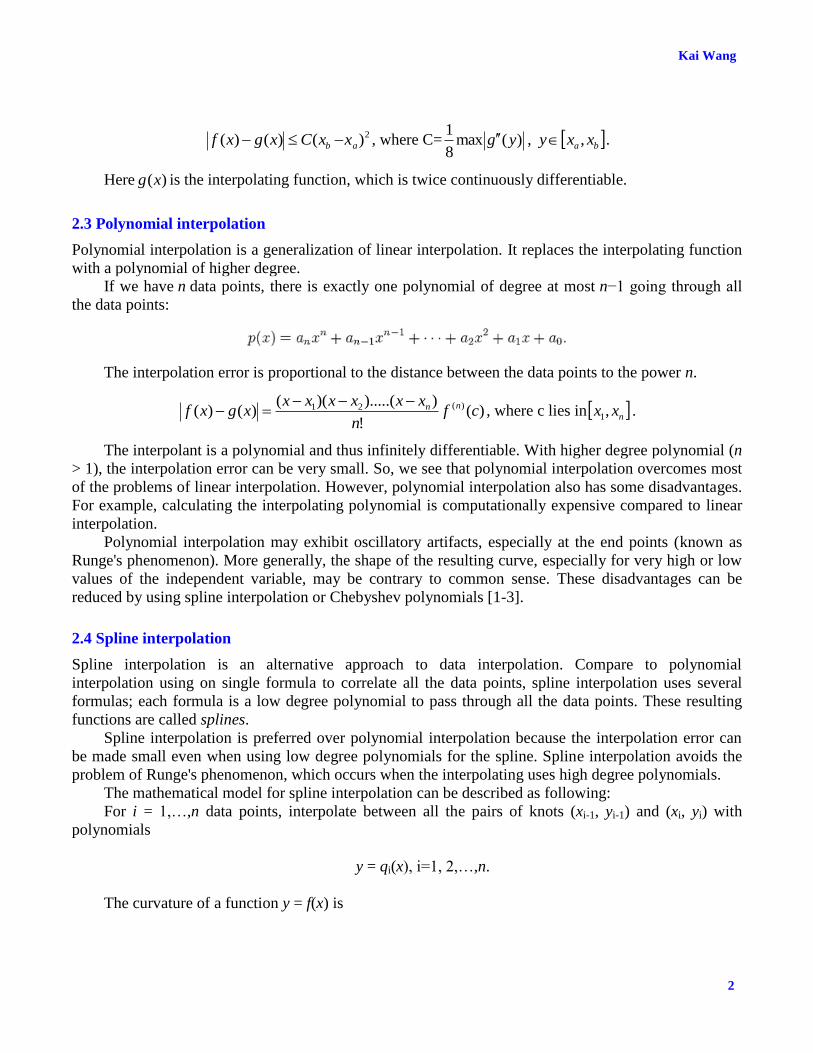
For example, data points (0,0), (1,0.5), (2, 1.8), (3,1.5), using the Matalab™ code for the solutions

above, construct the unique cubic spline (namely, natural spline) for the data points (see Fig. 1).

Kai Wang

8

Figure 1. The Natural Cubic Spline.

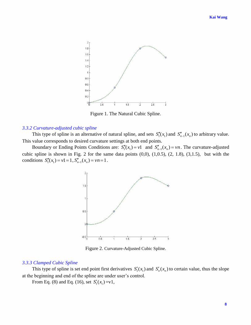
3.3.2 Curvature-adjusted cubic spline

This type of spline is an alternative of natural spline, and sets )( 11 xS and )(1 nn xS to arbitrary value.

This value corresponds to desired curvature settings at both end points.

Boundary or Ending Points Conditions are: 1)( 11 vxS and vnxS nn )(1 . The curvature-adjusted

cubic spline is shown in Fig. 2 for the same data points (0,0), (1,0.5), (2, 1.8), (3,1.5), but with the

conditions 11)( 11 vxS , 1)(1 vnxS nn .

Figure 2. Curvature-Adjusted Cubic Spline.

3.3.3 Clamped Cubic Spline

This type of spline is set end point first derivatives )( 11 xS and )( nn xS to certain value, thus the slope

at the beginning and end of the spline are under user’s control.

From Eq. (8) and Eq. (16), set )( 11 xS =v1,

9

A STUDY OF CUBIC SPLINE INTERPOLATION

)( 11 xS = 1b = )6

2( 2112 DDDD

hh

yy

We can have:

1DD =2

2

2

112

2

6)(6

h

DDhhbyy (21)

Also from equation 8 and 16, set )(1 nn xS = vn = 1nb ,

nDD =2

1

2

11 26)(6

h

DDhhbyy nnnn (22)

The clamped cubic spline is shown in Fig. 3 (below) for the same data points (0,0),(1,0.5), (2, 1.8),

(3,1.5), and )( 11 xS = 0.5, )(1 nn xS =0.5.

Figure 3. Clamped Cubic Spline.

3.3.4 Parabolically-Terminated Cubic Spline

For this type of spline, )(1 xS and )(1 xSn are forced to be the functions of degree 2, which means

that 1d = 1nd = 0.

From Eq. 15, h

DDDDd ii

i6

1 , therefore:

1d =1

12

6h

DDDD = 0, and 1DD = 2DD

1nd =1

1

6

n

nn

h

DDDD= 0, and 1 nn DDDD

The parabolically-terminated cubic spline is shown in Fig. 4 (below) for the same data points

(0,0),(1,0.5), (2, 1.8), (3,1.5).

Kai Wang

10

Figure 4 Parabolically-Terminated Cubic Spline

3.3.5 Not-a-Knot cubic spline

Two conditions 1d = 2d , 2nd = 1nd were added to construct the unique spline. )(1 xS and )(2 xS

already agree at zeros, first and second derivatives. The condition 1d = 2d causes )(1 xS and )(2 xS to be

identical cubic polynomials; thus the data-base point x2 is not needed anymore. Same thing is for

)(2 xSn and )(1 xSn , and data point xn-1.

From Eq. (15), h

DDDDd ii

i6

1 , therefore:

1d =1

12

6h

DDDD , 2d =

2

23

6h

DDDD , and 1d = 2d .

Hence, 1DD =2

2312

)(

h

DDDDhDD

.

Also, 2nd = 1nd ,

1nd =1

1

6

n

nn

h

DDDD, 2nd =

2

21

6

n

nn

h

DDDD, and therefore:

1

2

211 )(

n

n

nnnn DD

h

DDDDhDD

The not-a-knot cubic spline is shown below in Fig. 5 for data points (0,0), (1,0.5), (2, 1.8), (3,1.5), (4,0.8),

and n≥4.

11

A STUDY OF CUBIC SPLINE INTERPOLATION

Figure 5. Not-a-Knot Cubic Spline.

4. Cubic Spline Applications

4.1 Representing functions by approximating polynomials

First, let’s review the application of a cubic spline to approximate polynomials, or to evaluate a cubic

spline at certain point within the given interval [a, b].

As an example, consider the polynomial function )sin(1

)(2

xx

xf , on the interval [π/4, 3π/2]. We

can take few coupled data points: (π/4, 1.1463), (π/2, 0.4053), (3π/4, 0.1274), (π, 0), (5π/4, -0.0459),

(3π/2, -0.0450). With natural cubic spline, the interpolating function is shown as a solid line in Fig. 6

below. The exact values of the polynomial function f(x) (red markers) are also shown in Fig. 6.

Comparing the results, we can see that the cubic-spline interpolating function approximates the exact

function with a good accuracy.

Figure 6. Comparing the Natural Cubic Spline Interpolating Function and the Exact Solution.

Kai Wang

12

4.2 Data correlation and interpolation

Data interpolation is widely used in real world, especially with large volume of irregular data. Find

polynomial functions guide these data within certain interval, can greatly help with data analysis and

data predicting. Cubic splines could be used for finding an interpolation function to correlate data.

For example, in the chemical experiment, the following data was obtained (see arrays t and D

below and Fig. 7):

t = [0 0.1 0 .499 0.5 0.6 1.0 1.4 1.5 1.899 1.9 2.0]

D = [0 0.06 0.17 0.19 0.21 0.26 0.29 0.29 0.30 0.31 0.31]

We need to estimate the value D when t = 1.2. Using the natural cubic spline interpolation (the

formula ],[)()()()( 1

32

iiiiiiiiii xxonxxdxxcxxbyxS ), we found D = 0.27527649.

Figure 7. The Chemical Experiment Data, D = f(t).

Conclusions

In this paper, we have presented an overview of the methods of interpolation and especially the cubic

spline interpolation, which is widely used in numerous real-world applications. The study presents the

definition of cubic spline interpolation and properties of different types of cubic splines, including a

natural spline, a curvature-adjusted spline, a clamped spline, a parabolically-terminated spline, and a not-a-

knot spline. The spline construction formulas and corresponding Matlab™ codes were developed for

different types of cubic splines with excellent accuracy of calculation. Two general applications of cubic

spline interpolation were also analyzed.

References

1. Interpolation. Wikipedia. Retrieved October 22, 2013, from

http://en.wikipedia.org/wiki/Interpolation

13

A STUDY OF CUBIC SPLINE INTERPOLATION

2. Spline Interpolation. Wikipedia. Retrieved October 22, 2013, from

http://en.wikipedia.org/wiki/Spline_interpolation

3. Polynomial Interpolation. Wikipedia. Retrieved October 22, 2013, from

http://en.wikipedia.org/wiki/Polynomial_interpolation

4. Mathews, J. H., and Fink, K. K. Chapter 5: Curve Fitting. In: Numerical Methods Using Matlab,

4th edition, Pearson, 2004.

5. Introduction to Plotting with Matlab. Math Sciences Computing Center, University of Washington,

September, 1996. Retrieved October 22, 2013, from

http://www.math.lsa.umich.edu/~tjacks/tutorial.pdf

6. Friedman, J., Hastie, T., and Tibshirani, R. Chapter5: Splines and Applications. In: The Elements of

Statistical Learning. Retrieved October 22, 2013, from

http://www.cs.ubbcluj.ro/~csatol/mach_learn/bemutato/BagyiIbolya_SplinesAndApplications.pdf

7. Grandine, T. A. The Extensive Use of Splines at Boeing. SIAM News, Vol. 38, No. 4, May 2005.

Retrieved October 22, 2013, from http://www.me.ucsb.edu/~moehlis/ME17/splines.pdf

8. Cubic Spline Interpolation. Retrieved October 22, 2013, from

http://www.mathworks.com/help/curvefit/cubic-spline-interpolation.html

Apendix A: Matlab™ Code for the Project

% Calculation of spline coefficients % Calculates coefficients of cubic spline % Input: x,y vectors of data points % plus two optional extra data v1, vn

% Output: matrix of coefficients b1,c1,d1;b2,c2,d2;...

function coeff=Myproject(x,y,v1,vn) n=length(x); A=zeros(n-2,n-2); % matrix A is n-2xn-2 r=zeros(n-2,1); h=zeros(n-1,1);

for i=1:n-1 % define the deltas h(i) = x(i+1)-x(i); end

% load the A matrix for i=2:n-2 A(i,i-1)=1; end for i=1:n-2 A(i,i)=4; end for i=1:n-3 A(i,i+1)=1; end

%fprintf('display Matrix A\n'); %disp(A);

Kai Wang

14

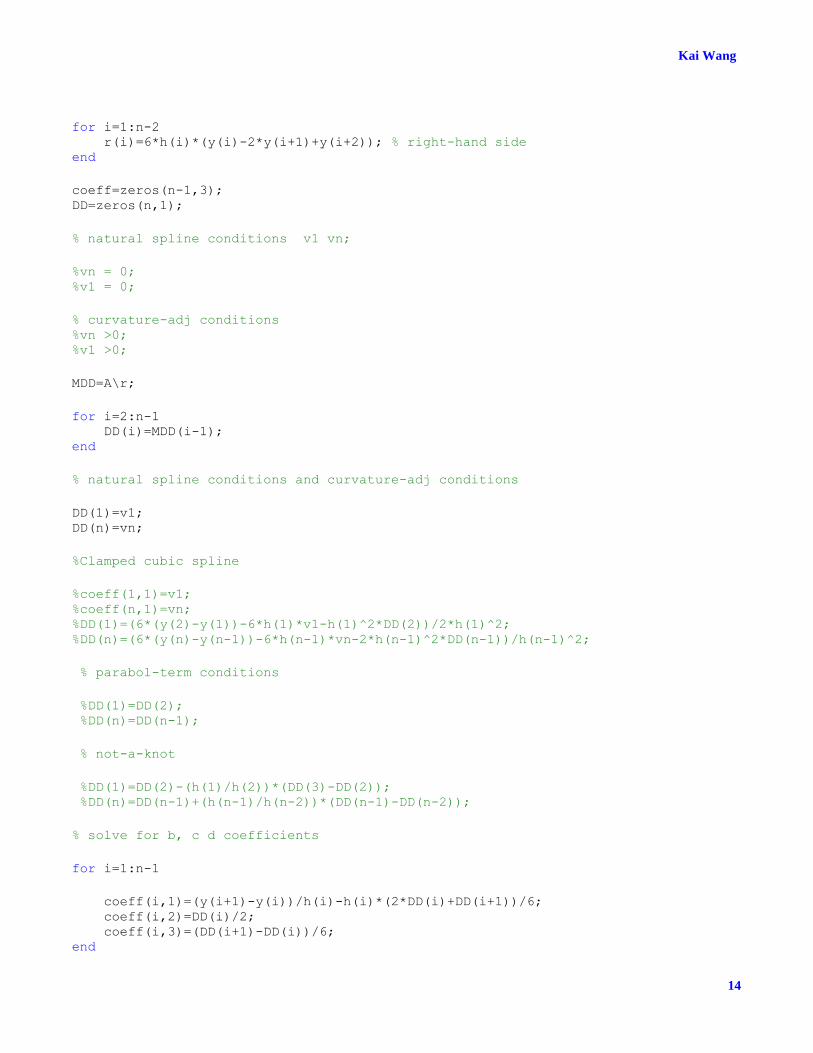
for i=1:n-2 r(i)=6*h(i)*(y(i)-2*y(i+1)+y(i+2)); % right-hand side end

coeff=zeros(n-1,3); DD=zeros(n,1);

% natural spline conditions v1 vn;

%vn = 0; %v1 = 0;

% curvature-adj conditions %vn >0; %v1 >0;

MDD=A\r;

for i=2:n-1 DD(i)=MDD(i-1); end

% natural spline conditions and curvature-adj conditions

DD(1)=v1; DD(n)=vn;

%Clamped cubic spline

%coeff(1,1)=v1; %coeff(n,1)=vn; %DD(1)=(6*(y(2)-y(1))-6*h(1)*v1-h(1)^2*DD(2))/2*h(1)^2; %DD(n)=(6*(y(n)-y(n-1))-6*h(n-1)*vn-2*h(n-1)^2*DD(n-1))/h(n-1)^2;

% parabol-term conditions

%DD(1)=DD(2); %DD(n)=DD(n-1);

% not-a-knot

%DD(1)=DD(2)-(h(1)/h(2))*(DD(3)-DD(2)); %DD(n)=DD(n-1)+(h(n-1)/h(n-2))*(DD(n-1)-DD(n-2));

% solve for b, c d coefficients

for i=1:n-1

coeff(i,1)=(y(i+1)-y(i))/h(i)-h(i)*(2*DD(i)+DD(i+1))/6; coeff(i,2)=DD(i)/2; coeff(i,3)=(DD(i+1)-DD(i))/6; end

15

A STUDY OF CUBIC SPLINE INTERPOLATION

%calculate the certain value on interval [a,b], i=6

%xd=1.2;

%Dt=y(6)+coeff(6,1)*(xd-x(6))+coeff(6,2)*(xd-x(6))^2+coeff(6,3)*(xd-x(6))^3;

%fprintf('%12.8f\n',xd,Dt);

%plot the figure after calculation.

clf;hold on; % clear figure window and turn hold on

for i=1:n-1 x0=linspace(x(i),x(i+1),100); dx=x0-x(i); y0=coeff(i,3)*dx; % evaluate using nested multiplication y0=(y0+coeff(i,2)).*dx; y0=(y0+coeff(i,1)).*dx+y(i); plot([x(i) x(i+1)],[y(i) y(i+1)],'o',x0,y0) end

% plot the (1/x^2)*sin(x)

%hold on

%x1=pi/4:0.1:3*pi/2; %y1=x1.^(-2).*sin(x1); %plot(x1, y1,'r*');

hold off end

___________________ * KAI WANG is a senior medical device and system product design engineer in Philips Healthcare Corp. He is a major

contributor to several prime medical projects on software systems design, development, test and implementation in Philips

Healthcare Corp. He completed Master Degree in Computer Science at Rivier University, Nashua, NH, in January

2014. He also holds B.S. Degree from Harbin University of Science and Technology and M.S. Degree from TianJin

University.