Page 1
Accepted Manuscript
A study of heat transfer in fluidized beds using an integrated DIA/PIV/IR tech-nique
Amit V. Patil, E.A.J.F. Peters, Vinayak S. Sutkar, N.G. Deen, J.A.M. Kuipers
PII: S1385-8947(14)01011-0DOI: http://dx.doi.org/10.1016/j.cej.2014.07.107Reference: CEJ 12475
To appear in: Chemical Engineering Journal
Please cite this article as: A.V. Patil, E.A.J.F. Peters, V.S. Sutkar, N.G. Deen, J.A.M. Kuipers, A study of heattransfer in fluidized beds using an integrated DIA/PIV/IR technique, Chemical Engineering Journal (2014), doi:http://dx.doi.org/10.1016/j.cej.2014.07.107
This is a PDF file of an unedited manuscript that has been accepted for publication. As a service to our customerswe are providing this early version of the manuscript. The manuscript will undergo copyediting, typesetting, andreview of the resulting proof before it is published in its final form. Please note that during the production processerrors may be discovered which could affect the content, and all legal disclaimers that apply to the journal pertain.
Page 2
A study of heat transfer in fluidized beds using an
integrated DIA/PIV/IR technique
Amit V. Patila, E. A. J. F. Petersa,∗, Vinayak S. Sutkara, N. G. Deena, J. A.M. Kuipersa
aMultiphase Reactors Group, Department of Chemical Engineering & Chemistry,Eindhoven University of Technology, P.O. Box 513, 5600 MB Eindhoven, the
Netherlands.
Abstract
A new measuring technique for studying heat transfer in gas-solid fluidized
beds is proposed using infrared (IR) thermography. An infrared camera is
coupled with a visual camera to simultaneously record images to give in-
stantaneous thermal and hydrodynamic data of a pseudo 2D fluidized bed.
The established techniques: digital image analysis (DIA) and particle image
velocimetry (PIV) are combined with IR thermography to obtain combined
quantitative (i.e. hydrodynamic and thermal) data sets. In this work, the
calibration procedure and the methods that are used to combine the data
obtained by the different techniques are discussed. The combined technique
provides insightful information on the heat transfer in a fluidized bed for
varying particle size, aspect ratio and background (or fluidization) gas veloc-
ity.
Keywords: multiphase flow, particle image velocimetry, digital image
analysis, infrared thermography, fluidized beds, heat transfer
∗Corresponding author. Tel: +31 40 247 3122; Fax: +31 40 247 5833Email address: [email protected] (E. A. J. F. Peters)
Preprint submitted to Chemical Engineering Journal July 31, 2014
Page 3
1. Introduction
Fluidized beds are encountered in a variety of industries because of their
favorable mass and heat transfer characteristics. Some of the prominent pro-
cessing applications include coating, granulation, drying, and synthesis of
fuels, base chemicals and polymers. Many of the important applications of
fluidized beds involve highly exothermic or endothermic reactions which give
rise to a high rate of heat removal or supply to the system. Fluidized catalytic
cracking, fluidized bed coal combustion and polymerisation for production
of polyethylene (UNIPOL) are some of the well known processes. Under
such conditions formation of hot spots or zones is a phenomenon which can
severely effect the overall performance of the reactor. Hence in depth knowl-
edge of the heat transfer processes in fluidized beds is highly relevant.
The hydrodynamics of fluidized beds has been investigated by many re-
searchers. Moreover extensive studies of heat transfer in fluidized beds have
been reported with many supporting theories proposed on the prevailing heat
transfer mechanism [1–7]. Most of the previous heat transfer research on flu-
idized beds involved the use of temperature probes placed inside or on the
walls of fluidized beds [8–10].
In recent years, infrared (IR) technique, a new noninvasive method for
measuring temperature in fluidized beds has been developed [11, 12]. Tsuji
et al. [11] proposed an idea of combining IR with PIV to study heat transfer
in fluidized beds. Infrared thermography has been used frequently in pro-
cess engineering research for heat transfer measurements and studies [13–16].
This measuring technique is quite well known to be reliable for non-insitu
2
Page 4
measurements. Recent work by Dang et al. [17] demonstrated the suitabil-
ity of an infrared camera (fitted with spectral filters) for CO2 concentration
measurement in gas voids inside pseudo 2D fluidized beds. This work builds
on the measuring method proposed by Tsuji et al. [11] using improved ex-
perimental and post processing techniques.
Some of the common techniques known for hydrodynamic studies are
electrical capacitance tomography, X-ray tomography, magnetic resonance
particle tracking or positron emission particle tracking and particle image
velocimetry (PIV). Among these the PIV technique is specifically used for
pseudo 2D beds and has the advantage of being non-intrusive, low cost com-
pared to other techniques and, for our purposes, can be easily coupled with
the infrared camera measuring technique for thermographic study. In stud-
ies of pseudo 2D fluidized beds digital image analysis (DIA) can be used to
determine local solid volume fractions. A combined PIV/DIA analysis as
developed by van Buijtenen et al. [18] and de Jong et al. [19] can be used to
determine the spatial distribution of the solids mass fluxes.
In our study the infrared technique is coupled with this PIV/DIA method.
PIV is performed with a high speed visual camera using two close consecutive
instantaneous images. Cross-correlation analysis on such image pairs give
velocity field data. DIA on one of the same image pairs provides the solid
volume fraction field data in the system. The coupling of DIA and PIV results
gives the solids mass fluxes. In this work the IR measurements are coupled
with the DIA and PIV measurements of the visual camera to obtain spatial
and instantaneous information on both solids motion and solids temperature
field in fluidized beds.
3
Page 5
The objective of this paper is twofold. First, the technical details such
as calibration and data-processing related to combining the three methods:
DIA, PIV and IR are communicated. Second, it is shown that this combi-
nation of measuring techniques can produce useful data sets to characterize
heat-transfer in pseudo-2D fluidized beds. The effects of particle size and
fluidization or background gas velocity on the heat transfer characteristics
are presented. The generated data sets can be used later for validating CFD
models.
2. Experimental set-up and procedures
2.1. Fluidized bed equipment
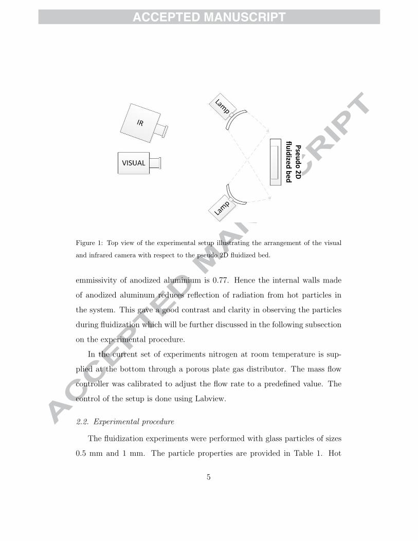
The experimental study is carried out on a small pseudo 2D fluidized bed.
A schematic view of the set up is shown in Fig 1. The fluidized bed is 8 cm
wide, 20 cm high and 1.5 cm in depth. The front wall of the fluidized bed is
made up of sapphire glass specifically chosen to give a high transmittance to
the infrared light.
The back and side walls consist of aluminium coated from the inside
with matt finish black paint to reduce reflection. The aluminium frame was
anodized to give the material better adhesion for paints and glue used to
attach the sapphire mirror and other accessories to the frame. It also provides
corrosion and wear resistance to the whole frame and helps to reduce charging
of the particles. The back aluminium frame was fitted with thermocouples
to measure its temperature at two different heights.
The polished aluminium has a low emmisivity of 0.09. This helps in
reducing any interference that may arise due to heating of the frame. The
4
Page 6
Figure 1: Top view of the experimental setup illustrating the arrangement of the visual
and infrared camera with respect to the pseudo 2D fluidized bed.
emmissivity of anodized aluminium is 0.77. Hence the internal walls made
of anodized aluminum reduces reflection of radiation from hot particles in
the system. This gave a good contrast and clarity in observing the particles
during fluidization which will be further discussed in the following subsection
on the experimental procedure.
In the current set of experiments nitrogen at room temperature is sup-
plied at the bottom through a porous plate gas distributor. The mass flow
controller was calibrated to adjust the flow rate to a predefined value. The
control of the setup is done using Labview.
2.2. Experimental procedure
The fluidization experiments were performed with glass particles of sizes
0.5 mm and 1 mm. The particle properties are provided in Table 1. Hot
5
Page 7
particles heated in an oven at 120 ◦C were charged into the empty bed at
room temperature, after which a constant gas stream at 20 ◦C is supplied
through the bottom plate.
Along with fluidizing the particles, the cold gas cools them in time. This
was recorded by the two cameras. The recording of the cameras was started
before charging of the particles and was continued for about 2-3 minutes.
This was approximately the time required by the fluidizing gas to cool the
particles in the system. We choose to cool the particles instead of heating
them up, because in this case the contrast between hot particles and cold
background is large initially. It was observed that the background effects
could be easily filtered and a high quality measurement was possible. This
will be discussed in detail later.
The glass particles used in the experiments were properly washed with
water and dried in order to make use of well-cleaned particles. To remove
any charging of particles during fluidization the particles were rinsed with
a Catanac solution. The Catanac solution was prepared by dissolving 1 ml
of Catanac SP antistatic agent into 100 ml of ethanol. The particles were
subsequently dried for one day producing glass particles with a coating of
Catanac. Some rinsed particles in this solution were also fluidized in the set
up so that small amount of Catanac coated the interior of the fluidized bed.
For this work 2 different particle sizes of 0.5 mm and 1 mm were used,
which are Geldart B and Geldart D type particles. For the 1 mm particles two
bed-heights corresponding to a bed mass of 75 g and 125 g were considered.
Three background gas velocities were used. The properties and settings for
the fluidization experiments are summarized in Table 1.
6
Page 8
Table 1: Particle properties and settings used in the experiments.
Particle ma-
terial
Glass
Particle den-
sity ρp
2500 kg/m3
Norm. coeff.
of restit.
0.97
Tang. coeff.
of restit.
0.33
Fluid heat ca-
pacity Cp,f
1010 J/kgK
particle heat
capacity Cp,p
840 J/kgK
dp Geldart
type
ubg umf Bed mass
(mm) (m/s) (m/s) (g)
0.5 B 0.51 0.18 75
0.5 B 0.86 0.18 75
1.0 D 1.20 0.58 75 & 125
1.0 D 1.54 0.58 75 & 125
1.0 D 1.71 0.58 75 & 125
7
Page 9
2.3. Camera setup
The fluidization was recorded by a high speed visual camera (La Vision
ImagePro, 560 × 1280 resolution) and an infrared camera (FLIR SC7600,
250 × 512 resolution). The IR camera was sensitive in the 1.5 - 5.1 µm
spectral range. The cameras were placed on a tripod in front of the fluidized
bed. To minimise the difference in views the cameras were placed as close
as possible. The set up was illuminated using a pair of white LED lamps.
White LED have blue and yellow peaks in the spectrum, but have very low
intensity in the infrared band. Therefore the lights do not interfere with the
IR thermography. The lamps were placed at an angle of 45◦ with respect
to the normal of the fluidized bed. This reduces effects like reflection and
shining on the fluidized bed. See Fig. 1 for details.
The visual camera had an exact front view of the sapphire window, but
the IR camera was placed at a small angle. The reason for placing the IR
camera at an angle is that the IR camera is internally cooled and its lens is
obviously transparent to infrared radiation. Due to its low temperature the
radiation leaving the camera through its lens was quite different from the
radiation of the surroundings that roughly corresponds to room temperature
black-body radiation. A small part of the radiation that the IR camera
detects was due to reflections of radiation of the surroundings. Combining
these facts means that, when placing the camera fully perpendicular to the
sapphire window, a cold spot would be visible.
The visual and infrared cameras were connected to the computer system
via a trigger box system. During the high signal the cameras were in capture
mode. The trigger box sends simultaneous (or with a small preset delay)
8
Page 10
pulses to both the visual camera and the IR camera, which ensures that the
two cameras record images at the same instant in time. In this way we can
map the thermographic data (heat transfer) on the hydrodynamic data and
perform a complete coupled study of heat transfer and concurrent gas-solid
flow.
An example of the captured frames alongside a signal diagram represent-
ing the trigger based capture mechanism is shown in Fig. 2. The images
were recorded at a 10 Hz frequency, so the time for one cycle was 100 ms.
During one cycle the IR camera makes one recording using an integration
time of 600 µs and the visual camera two recordings of an exposure time
of 700 µs with 100 µs delay in between. The two consecutive visual images
were needed for the PIV measurements. The time difference between the two
images used in the velocity calculation is the sum of the exposure time and
the delay time, i.e. 800 µs.
The term ‘integration time’ is commonly used for the exposure time of the
thermal imaging detector inside the IR camera to produce a single frame. A
large integration time increases the contrast, and therefore the temperature
difference that can be detected, but it should not be so large that pixels get
saturated. By using an integration time of 600 µs the temperature range
of 30 - 100 ◦C was well represented. The raw output of the IR camera is
represented by a digital level (DL) signal, which is a 14 bit number (so the
maximum is 16383) for each pixel.
9
Page 11
(a) trigger system signal diagram (b) visual image
0C
35
40
45
50
55
60
65
70
75
80
85
(c) infrared image
Figure 2: Trigger signal mechanism and example of raw synchronized visual and infrared
snapshots with 1 mm particles, 1.2 m/s background velocity and 125 g bed mass.
3. Measuring techniques
3.1. Particle image velocimetry (PIV)
The PIV method used here was fairly standard and for example exten-
sively described in literature [18, 19]. The visual image has a size of 560×1168
pixels. The PIV performed here uses a multi-pass algorithm using an in-
terrogation window of 32 × 32 with 50 % overlap for computing the cross
correlations. This results in a post processed velocity field on a 35× 73 grid
for the pseudo 2D bed. A standard median filter was used to remove outliers
from the vector field.
3.2. Digital image analysis (DIA)
The DIA involved a series of processing steps that was aimed at computing
the 3D solids volume fractions. The DIA procedure used was similar to that
described by de Jong et al. [19]. The raw visual 2D digital image consisted
of pixels with different intensities. During DIA this image was subjected to
10
Page 12
a set of preprocessing steps, namely: background substraction, elimination
of overexposed and underexposed pixels. A raw preprocessed image is shown
in Fig. 3a.
This digital image was then corrected for inhomogeneity and normalized
between 0 and 1. Here 1 is representative of the brightest particle and 0 of the
background or no particle. The normalized values of the 2D image were then
averaged over an interrogation window (of 32 × 32) to get the apparent 2D
volume fraction of the particles (represented by ε2D). This 2D solid volume
fraction was translated to the 3D volume fraction using the correlation,
ε3D =
Aε2D (1− ε2D/B)−1 for ε3D < ε3D,max
ε3D,max for ε3D > ε3D,max
(1)
This correlation was proposed by de Jong et al. [19] using results from discrete
element method simulations. In this equation we take ε3D,max = 0.6, to be
the maximum solids volume fraction. According to de Jong et al. [19] the
parameter A is related to the bed depth ∆z and the particle diameter dp, as
A = 1.028∆z/dp. This relation was obtained by using DEM (discrete element
method) simulation results to generate images and perform DIA on them.
The remaining fitting parameter B is determined such that the deviation
between the computed bed mass and the experimental bed mass is minimal.
The computed bed mass was calculated from ε3D by multiplication with the
solids density and subsequent integration over the bed volume.
3.3. Thermography and IR camera calibration
The fate of incident radiation on an object is determined by three wave-
length dependent fractions, namely, absorptance, reflectivity and transmit-
11
Page 13
100 200 300 400 500
100
200
300
400
500
600
700
800
900
1000
1100
0
50
100
150
200
250
300
350
400
(a) Preprocessed back-
ground removed image
Normalised
100 200 300 400 500
100
200
300
400
500
600
700
800
900
1000
1100
0
0.1
0.2
0.3
0.4
0.5
0.6
0.7
0.8
0.9
(b) Normalized 2D parti-
cle fraction
10 20 30
10
20
30
40
50
60
0
0.1
0.2
0.3
0.4
0.5
0.6
(c) 3D particle fraction
Figure 3: DIA processing of visual images showing the 3 major steps of the analysis:
preprocessing, determining ε2D, converting ε2D → ε3D. The images shown are from a
fluidization run of particle size 1 mm, background gas velocity 1.2 m/s and bed mass 75 g.
tance. For example, the amount of adsorbed radiation equals the absorptance
times the intensity of the incoming radiation at that wavelength. For emitted
radiation we have a fourth factor that is of importance, namely, the emis-
sivity. The amount of emitted radiation at a specific wavelength is equal
to the emissivity times the black-body radiation intensity corresponding to
that wavelength. Kirchhoff’s thermal law of radiation states that emissivity
equals absorptance.
Since either the radiation is absorbed or reflected or transmitted we have
a(λ) + r(λ) + τ(λ) = 1. For the use of thermography objects of which one
wants to determine the temperature should have an emissivity close to 1
in the IR regime. For example for glass we have an emissivity of 0.8 −
0.95 in the full IR spectrum of our camera. This means that, for these
12
Page 14
IR wavelengths, already after a few interactions with matter most of this
radiation has been absorbed and re-emitted as thermal (i.e. black-body)
radiation. If, as in our case, we have hot glass beads then the major part
of the radiation coming from these particles is due to the emission of these
particles, i.e., the emissivity times the black-body intensity corresponding to
the particle temperature.
The remaining radiation coming from a particle is due to reflections of
radiation from other sources. Part of this reflected radiation originates from
neighboring particles that are similarly hot, and another part comes from
the room temperature surroundings. On its way from a glass bead of which
we want to measure the temperature to the IR camera the radiation might
interact with other matter.
For an object that should be transparent for the IR radiation, like the
window of the bed, the transmittance should be close to 1. Clearly using
a glass window, with its high absorptance, would ruin the measurement.
Therefore we used a sapphire window which has a transmittance of about
0.9. The distance between the fluidized bed and the camera was so small that
the air in between was fully IR transparent to very good approximation. In
the end, the radiation that enters the IR camera apparently coming from a
glass bead is composed of thermal radiation coming directly from a particle
(say 80 %) and the remainder of the radiation is a complicated mixture of
radiative contribution from either reflected or emitted by another object.
The used FLIR SC7600 camera was calibrated using perfect black-body
radiation. So for black-body objects it can correlate radiation and temper-
ature in a very accurate way. For ‘real’ objects the manufacturer supplied
13
Page 15
(a) IR snapshot during pouring of hot
particles showing: tracer particle visible
(b) IR image during calibration: tracer
particle invisible
Figure 4: IR images demonstrating the calibration procedure
software can perform a correction assuming a value of the emissivity of the
objects plus the assumption that all other radiation is black-body radiation
at room temperature. For both the emissivity and the room temperature the
user needs to supply values.
Because the model used by the FLIR software was not a perfect repre-
sentation of reality we chose to perform our own calibration for our specific
situation. For this calibration a glass particle was fitted at the tip of a
thermocouple probe. This particle was placed inside the bed very close to
the sapphire glass so that it was visible for the IR camera. The calibration
started by pouring hot particles into the bed. Immediately after the pouring
the colder tracer particle could be easily distinguished from the other hotter
particle as seen in the infrared image of the bed. Fig. 4a shows the recorded
14
Page 16
3000 5000 7000 9000 11000 1300030
40
50
60
70
80
90
100
110
DL
Tem
peratu
re o
f th
erm
oco
up
le, K
Calibration experiment data
model fit
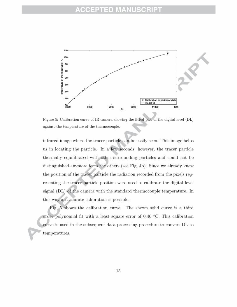
Figure 5: Calibration curve of IR camera showing the fitted plot of the digital level (DL)
against the temperature of the thermocouple.
infrared image where the tracer particle can be easily seen. This image helps
us in locating the particle. In a few seconds, however, the tracer particle
thermally equilibrated with other surrounding particles and could not be
distinguished anymore form the others (see Fig. 4b). Since we already knew
the position of the tracer particle the radiation recorded from the pixels rep-
resenting the tracer particle position were used to calibrate the digital level
signal (DL) of the camera with the standard thermocouple temperature. In
this way an accurate calibration is possible.
Fig. 5 shows the calibration curve. The shown solid curve is a third
order polynomial fit with a least square error of 0.46 ◦C. This calibration
curve is used in the subsequent data processing procedure to convert DL to
temperatures.
15
Page 17
0C
30
35
40
45
50
55
60
65
70
75
(a) distance from bed:
1.4 cm
0C
30
35
40
45
50
55
60
65
70
75
(b) distance from bed:
0.7 cm
0C
30
35
40
45
50
55
60
65
70
75
(c) distance from bed:
0.1 cm
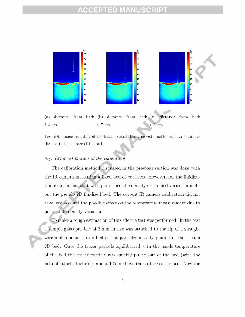
Figure 6: Image recording of the tracer particle being moved quickly from 1.5 cm above
the bed to the surface of the bed.
3.4. Error estimation of the calibration
The calibration method discussed in the previous section was done with
the IR camera measuring a fixed bed of particles. However, for the fluidiza-
tion experiments that were performed the density of the bed varies through-
out the pseudo 2D fluidized bed. The current IR camera calibration did not
take into account the possible effect on the temperature measurement due to
particulate density variation.
To make a rough estimation of this effect a test was performed. In the test
a sample glass particle of 2 mm in size was attached to the tip of a straight
wire and immersed in a bed of hot particles already poured in the pseudo
2D bed. Once the tracer particle equilibrated with the inside temperature
of the bed the tracer particle was quickly pulled out of the bed (with the
help of attached wire) to about 1.5cm above the surface of the bed. Now the
16
Page 18
particle was lowered quickly back towards the top surface of the bed till it
came in contact with the bed. This process was recorded with the IR camera
at a high frequency of 100 Hz. A small background gas velocity of 0.1 m/s
was maintained so that when the particle is lifted above the bed it is in a
gas environment that has a temperature equal to the bulk temperature of
the bed. Fig. 6 shows three images that were recorded while lowering the
tracer particle. The temperature recorded at the centre of the particle was
extracted using the calibration curve. With this data a plot of temperature
of the tracer particle against the distance of the particle from the top surface
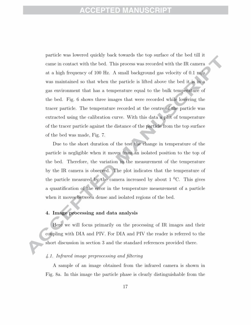
of the bed was made, Fig. 7.
Due to the short duration of the test the change in temperature of the
particle is negligible when it moves from an isolated position to the top of
the bed. Therefore, the variation in the measurement of the temperature
by the IR camera is observed. The plot indicates that the temperature of
the particle measured by the camera increased by about 1 0C. This gives
a quantification of the error in the temperature measurement of a particle
when it moves between dense and isolated regions of the bed.
4. Image processing and data analysis
Here we will focus primarily on the processing of IR images and their
coupling with DIA and PIV. For DIA and PIV the reader is referred to the
short discussion in section 3 and the standard references provided there.
4.1. Infrared image preprocessing and filtering
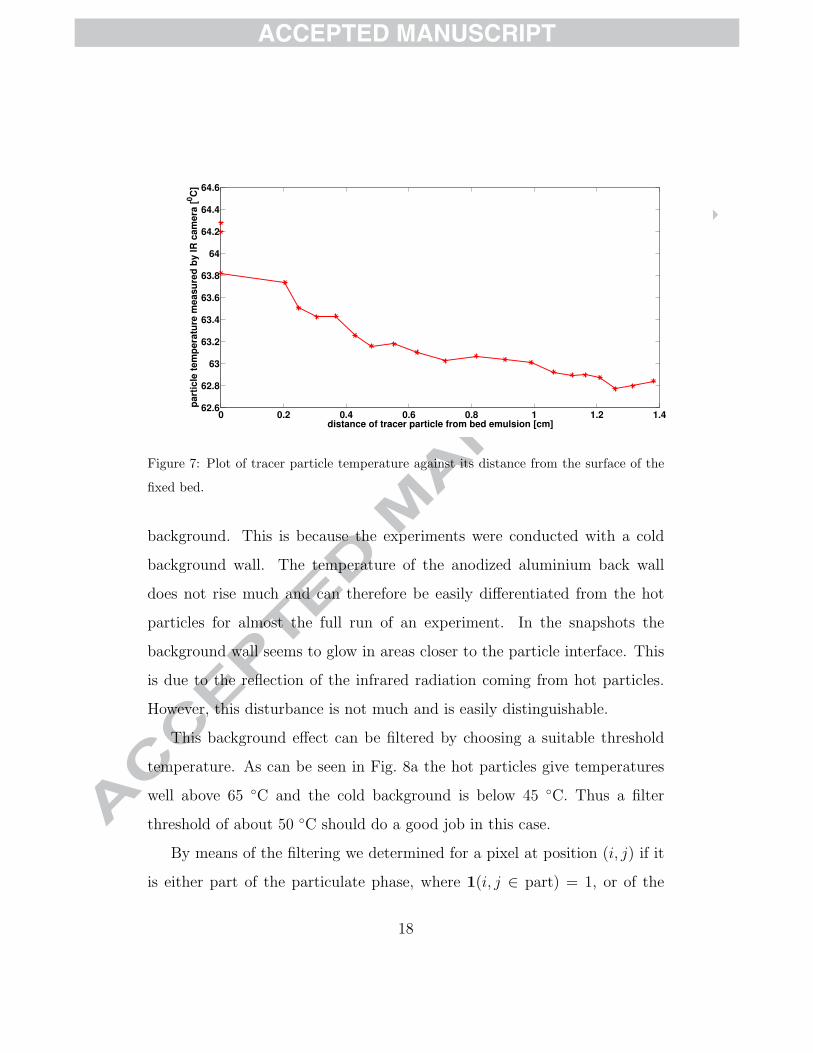
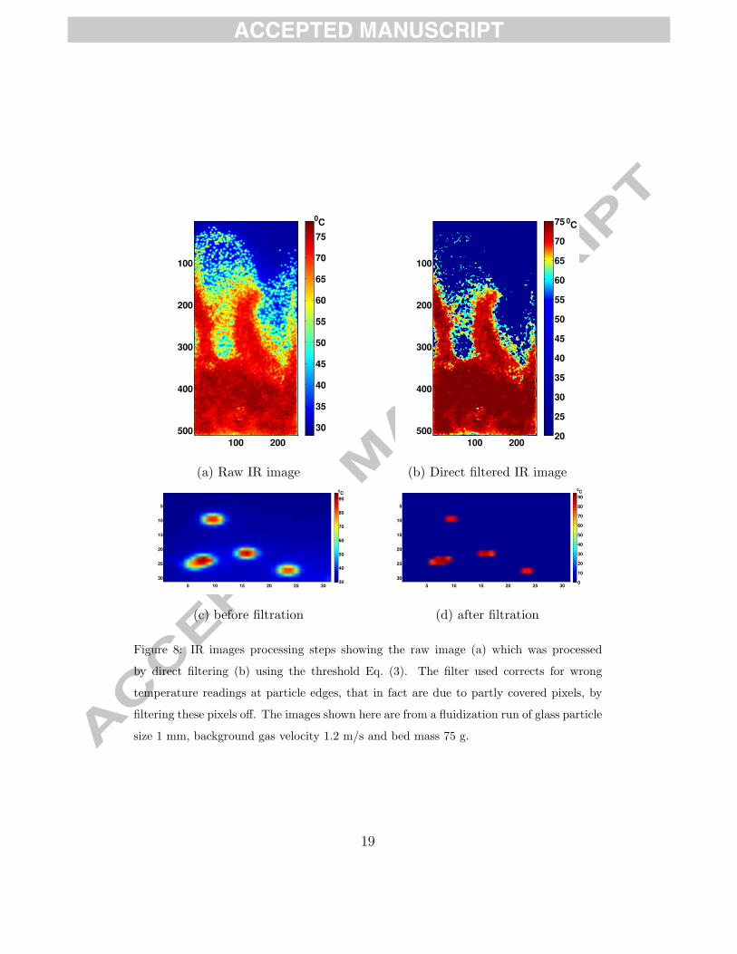
A sample of an image obtained from the infrared camera is shown in
Fig. 8a. In this image the particle phase is clearly distinguishable from the
17
Page 19
0 0.2 0.4 0.6 0.8 1 1.2 1.462.6
62.8
63
63.2
63.4
63.6
63.8
64
64.2
64.4
64.6
distance of tracer particle from bed emulsion [cm]
parti
cle
tem
peratu
re m
easu
red
by IR
cam
era [
0C
]
Figure 7: Plot of tracer particle temperature against its distance from the surface of the
fixed bed.
background. This is because the experiments were conducted with a cold
background wall. The temperature of the anodized aluminium back wall
does not rise much and can therefore be easily differentiated from the hot
particles for almost the full run of an experiment. In the snapshots the
background wall seems to glow in areas closer to the particle interface. This
is due to the reflection of the infrared radiation coming from hot particles.
However, this disturbance is not much and is easily distinguishable.
This background effect can be filtered by choosing a suitable threshold
temperature. As can be seen in Fig. 8a the hot particles give temperatures
well above 65 ◦C and the cold background is below 45 ◦C. Thus a filter
threshold of about 50 ◦C should do a good job in this case.
By means of the filtering we determined for a pixel at position (i, j) if it
is either part of the particulate phase, where 1(i, j ∈ part) = 1, or of the
18
Page 20
0C
100 200
100
200
300
400
500 30
35
40
45
50
55
60
65
70
75
(a) Raw IR image
0C
100 200
100
200
300
400
50020
25
30
35
40
45
50
55
60
65
70
75
(b) Direct filtered IR image0C
5 10 15 20 25 30
5
10
15
20
25
3030
40
50
60
70
80
90
(c) before filtration
0C
5 10 15 20 25 30
5
10
15
20
25
300
10
20
30
40
50
60
70
80
90
(d) after filtration
Figure 8: IR images processing steps showing the raw image (a) which was processed
by direct filtering (b) using the threshold Eq. (3). The filter used corrects for wrong
temperature readings at particle edges, that in fact are due to partly covered pixels, by
filtering these pixels off. The images shown here are from a fluidization run of glass particle
size 1 mm, background gas velocity 1.2 m/s and bed mass 75 g.
19
Page 21
background for which 1(i, j ∈ part) = 0. Using this notation a pixel averages
were computed as
〈Tp〉pix =
∑i,j 1(i, j ∈ part)Tp(i, j)∑
i,j 1(i, j ∈ part)(2)
We find that the temperature distribution in the particulate phase is quite
narrow. Therefore a threshold closer to the average temperature than to the
background temperature, Tbg was used, namely,
Tthr = 0.25Tbg + 0.75 〈Tp〉pix. (3)
This relation was found to be suited by trial and error experimentation.
The background subtraction was found to be insensitive to the precise choice
of the parameters for defining the threshold temperature. For example, the
combinations of weights: (0.2, 0.8) and (0.3, 0.7) gave nearly the same results.
Since we use the threshold to compute the pixel-averaged temperature
Eq. (3) is an implicit definition. However, this average temperature only
changes slowly from one snapshot to the next. Therefore we used the av-
erage value, 〈Tp〉pix, from the previous time step to compute the threshold
temperature.
Fig. 8b shows the filtered image corresponding to Fig. 8a using Eq. (3).
Clearly, many of the shades that are present in Fig. 8a at the interface of the
particle phase are filtered off. This is due to edge filtering induced by Eq. (3)
and is desirable.
This is more clearly illustrated in the following two figures Fig. 8c and
Fig. 8d where some particles in flight are shown. The centers of the particles
show a high temperature and can be easily differentiated from the background
which has a faint glow because of the particles in its vicinity. At the edges of
20
Page 22
particles, however, there is a signal intensity in between that of the core of a
particles and the background. By using the calibration curve this digital level
erroneously translated into an in-between temperature. The real cause of the
in-between signal was that pixels representing the edges of particles were only
partly covered by particles. Since the lower signal does not translate into the
correct temperature it was better to filter partly covered pixels off. This
was done to a large extent by choosing the threshold relatively close to the
average particle temperature as done in Eq. (3).
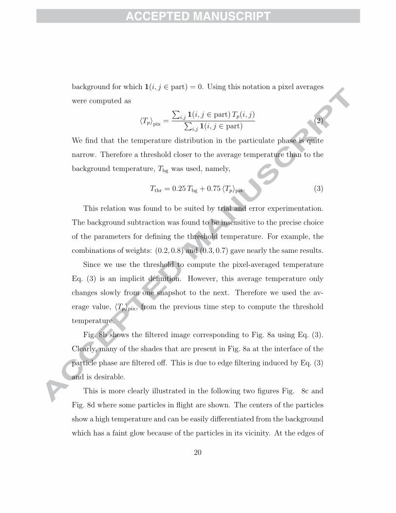
In Fig. 9 the mean pixel temperatures is plotted against time to give
the cooling profile for fluidized bed runs with 1 mm particle size and bed
mass 75 g for different background gas velocities. The starting point for the
recording was taken to be the point in time where the mean pixel tempera-
ture falls below 100 ◦C. The figure gives a closeup view of the region of the
temperature interval between 70 to 40 ◦C.
For each velocity the experiment was repeated 4 times. The repetitions
are shown using different symbols but the same color. The fluctuations be-
tween the repeated experiments at the same background velocity are less
than the separation of curves corresponding to different background veloc-
ities. This plot clearly shows that experiments are reproducible and that
the cooling curves for each of the background velocities are distinguishably
different.
4.2. DIA / IR coupling
The mean pixel temperature calculated in the previous section was not a
useful quantity for studying heat transfer. Changes in enthalpy are propor-
tional to the mass times heat capacity times temperature difference. Consid-
21
Page 23
6 8 10 12 14 16 18 20 22
45
50
55
60
65
70
75
80
time t, s
Mean
pix
el te
mp
eratu
re <
Tp>
pix
, C
ubg
= 1.71 m/s
ubg
= 1.54 m/s
ubg
= 1.2 m/s
Figure 9: Mean pixel temperature as defined in Eq. (2) with respect to time. Cooling curves
for bed with bed mass equal to 75 g and 1 mm sized particles for different background gas
velocities are shown.
ering that heat capacities and specific densities are nearly constant a mean
temperature that is calculated by a weighted-averaging using solids volume
fractions is more appropriate.This quantity can be computed by coupling IR
temperature fields with the DIA 3D volume fraction data of the bed.
The DIA process described earlier uses a high resolution 2D image (560×
1168) (size = 0.143 mm/pixel) shown in Fig. 3b to get the 3D particle fraction
data at a coarse grid (35× 73) (size 2.29 mm/pixel) also called interrogation
grid. In order to couple the 3D particle-fraction data of DIA with IR the high
resolution filtered IR image (250 × 512) (size = 0.312 mm/pixel) of Fig. 8b
was also divided into interrogation areas such that they produce grids of the
same size as that of DIA. So, each IR interrogation window has a size of
(250/35 × 512/73) pixels. The mean particulate pixel temperature in each
22
Page 24
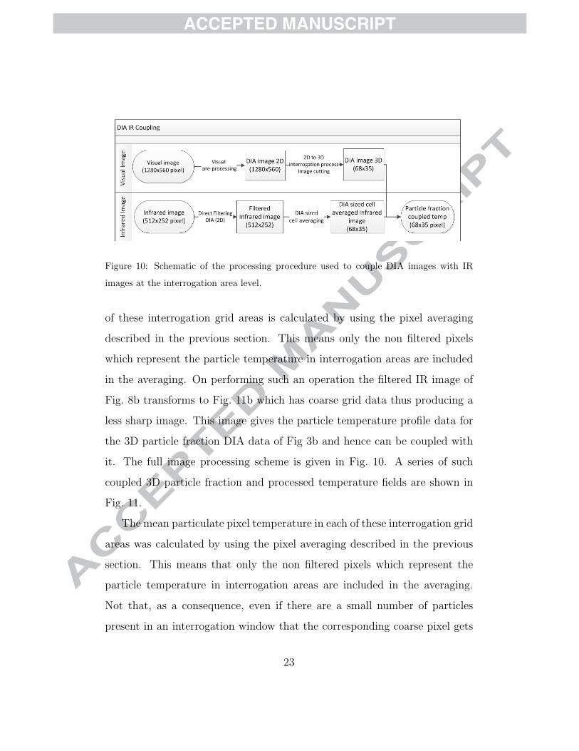
Figure 10: Schematic of the processing procedure used to couple DIA images with IR
images at the interrogation area level.
of these interrogation grid areas is calculated by using the pixel averaging
described in the previous section. This means only the non filtered pixels
which represent the particle temperature in interrogation areas are included
in the averaging. On performing such an operation the filtered IR image of
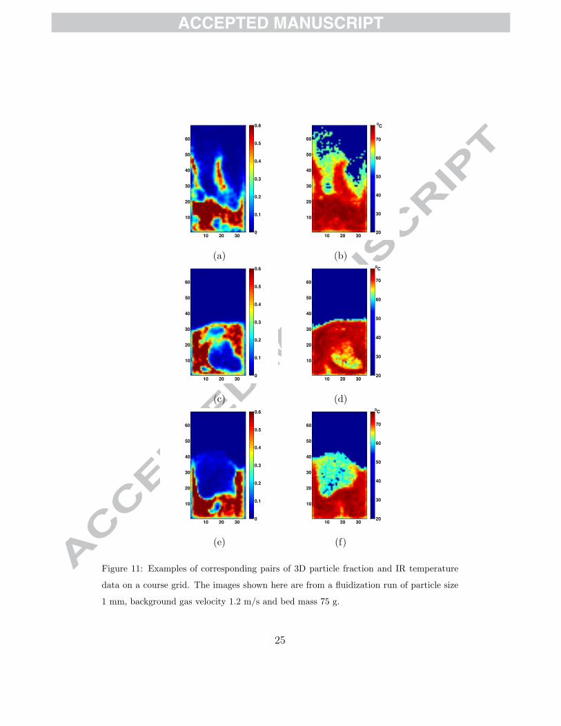
Fig. 8b transforms to Fig. 11b which has coarse grid data thus producing a
less sharp image. This image gives the particle temperature profile data for
the 3D particle fraction DIA data of Fig 3b and hence can be coupled with
it. The full image processing scheme is given in Fig. 10. A series of such
coupled 3D particle fraction and processed temperature fields are shown in
Fig. 11.
The mean particulate pixel temperature in each of these interrogation grid
areas was calculated by using the pixel averaging described in the previous
section. This means that only the non filtered pixels which represent the
particle temperature in interrogation areas are included in the averaging.
Not that, as a consequence, even if there are a small number of particles
present in an interrogation window that the corresponding coarse pixel gets
23
Page 25
the temperature corresponding to the average temperature of these particles.
This explains why in, e.g., the visual image Fig. 11e a region that contains
very little particles still has a high temperature in Fig. 11f.
The temperature distribution obtained from the pseudo 2D bed from the
IR images were that of the particles of the few front layers closest to the
sapphire window. Since this was a fluidized bed in operation it was expected
that in the depth direction the mixing was effective and the temperature was
nearly uniform. We know however that the particle distribution within the
fluidized bed was not uniform. Throughout the bed the particle fractions will
vary in time and space. As said, a temperature that was weighted with the
solids volume fraction was essential to understand heat transport phenomena
in fluidized beds. The solids-volume-fraction weighted spatial average was
computed as
〈Tp〉ε =
∑i,j εp(i, j)Tp(i, j)∑
i,j εp(i, j). (4)
Because of correlations between voidage and temperature it can be markedly
different from a pixel-averaged temperature. In fact the mean temperature
of particles computed by Eq. (4) mostly produces a higher value compared
to mean pixel temperature of Eq. (2) as the dense regions of the bed are
generally at a higher temperature compared to bubble regions or sparse par-
ticulate region. This can be observed in the corresponding DIA and IR
images of Fig. 11.
Fig. 12 shows the mean temperature plot using both methods for a flu-
idization experiment where this phenomenon can be clearly seen. Due to
the constant expansion and contraction of the bed the mean pixel tempera-
ture curve has much more fluctuation compared to solids-fraction weighted
24
Page 26
10 20 30
10
20
30
40
50
60
0
0.1
0.2
0.3
0.4
0.5
0.6
(a)
0C
10 20 30
10
20
30
40
50
60
20
30
40
50
60
70
(b)
10 20 30
10
20
30
40
50
60
0
0.1
0.2
0.3
0.4
0.5
0.6
(c)
0C
10 20 30
10
20
30
40
50
60
20
30
40
50
60
70
(d)
10 20 30
10
20
30
40
50
60
0
0.1
0.2
0.3
0.4
0.5
0.6
(e)
0C
10 20 30
10
20
30
40
50
60
20
30
40
50
60
70
(f)
Figure 11: Examples of corresponding pairs of 3D particle fraction and IR temperature
data on a course grid. The images shown here are from a fluidization run of particle size
1 mm, background gas velocity 1.2 m/s and bed mass 75 g.
25
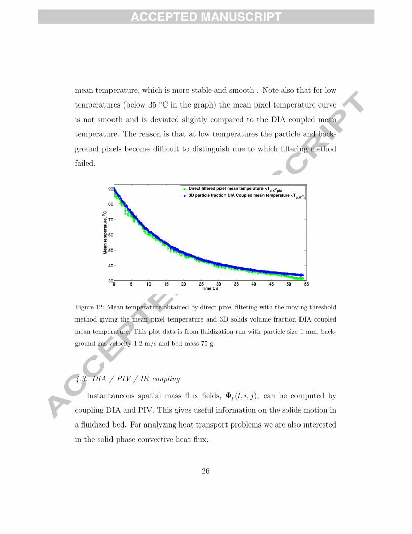
Page 27
mean temperature, which is more stable and smooth . Note also that for low
temperatures (below 35 ◦C in the graph) the mean pixel temperature curve
is not smooth and is deviated slightly compared to the DIA coupled mean
temperature. The reason is that at low temperatures the particle and back-
ground pixels become difficult to distinguish due to which filtering method
failed.
0 5 10 15 20 25 30 35 40 45 50 5530
40
50
60
70
80
90
Time t, s
Mean
tem
peratu
re,
0C
Direct filtered pixel mean temperature <Tp,X
>pix
3D particle fraction DIA Coupled mean temperature <Tp,X
>ε
Figure 12: Mean temperature obtained by direct pixel filtering with the moving threshold
method giving the mean pixel temperature and 3D solids volume fraction DIA coupled
mean temperature. This plot data is from fluidization run with particle size 1 mm, back-
ground gas velocity 1.2 m/s and bed mass 75 g.
4.3. DIA / PIV / IR coupling
Instantaneous spatial mass flux fields, ΦΦΦp(t, i, j), can be computed by
coupling DIA and PIV. This gives useful information on the solids motion in
a fluidized bed. For analyzing heat transport problems we are also interested
in the solid phase convective heat flux.
26
Page 28
This quantity can be obtained by complete coupling of the DIA data
(particle fraction), PIV data (particle velocity) and IR data (particle tem-
perature). The enthalpy change of a particle when its temperature changes
equals mpCp,p ∆Tp. So, when analysing heat transport the convective trans-
port of Tp can provide valuable information. We define an instantaneous
‘heat’ flux for each course grid position (i.e., interrogation window) as
Hp(t, i, j) = εp(t, i, j) ρpCp,p vp(t, i, j)Tp(t, i, j). (5)
4.4. Temperature distribution of particles
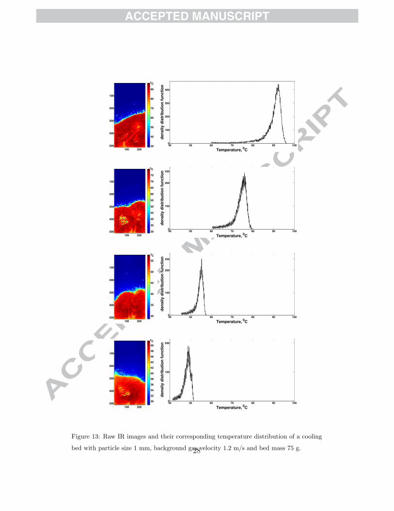
The infrared image observations that were made during a sample run are
shown in Fig. 13 together with temperature histograms. These distributions
have a well defined single peak. It was observed that the distribution spread
tended to become narrow as the cooling proceeded. This is expected because
at higher particle temperatures the difference between particles and inlet gas
is larger, which causes the temperature differences between mixing particles
to be also larger.
Besides the mean temperature, Eq. (4), the width of the distributions can
be characterized from the standard deviation, σp, which equals the square
root of the variance,
σ2p =
⟨(Tp − 〈Tp〉ε
)2⟩ε
=
∑i,j εp(i, j) (Tp(i, j)− 〈Tp〉ε)2∑
i,j εp(i, j)(6)
To obtain an impression of the relation between the bed temperature and
the width of the temperature distribution σp was plotted against the mean
particle temperature in Fig. 14a in an absolute and a relative way. These
plots clearly demonstrate the decreasing standard deviation as the bed cools
down.
27
Page 29
0C
100 200
100
200
300
400
500 30
40
50
60
70
80
90
40 50 60 70 80 90 1000
100
200
300
400
Temperature, 0C
de
ns
ity
dis
trib
uti
on
fu
nc
tio
n
0C
100 200
100
200
300
400
500 30
35
40
45
50
55
60
65
70
75
40 50 60 70 80 90 1000
100
200
250
Temperature, 0C
de
ns
ity
dis
trib
uti
on
fu
nc
tio
n
0C
100 200
100
200
300
400
50030
35
40
45
50
55
40 50 60 70 80 90 1000
100
200
250
Temperature, 0C
de
ns
ity
dis
trib
uti
on
fu
nc
tio
n
0C
100 200
100
200
300
400
50030
32
34
36
38
40
42
44
46
48
50
40 50 60 70 80 90 1000
100
200
Temperature, 0C
de
ns
ity
dis
trib
uti
on
fu
nc
tio
n
Figure 13: Raw IR images and their corresponding temperature distribution of a cooling
bed with particle size 1 mm, background gas velocity 1.2 m/s and bed mass 75 g.28
Page 30
In the relative plot the standard deviation is normalized by the thermal
‘driving force’ for the cooling process: 〈Tp〉ε− Tg,in. Fig. 14b shows that this
normalized standard deviation is more or less constant. These results also
show a large fluctuation in the standard deviation when the driving force is
high.
4.5. Time-averaging
Besides spatial averaging also time-averages per pixel give valuable infor-
mation. We will use an overbar-notation to distinguish time-averaging from
spatial averaging,
εp(i, j) =1
Nt
∑t
εp(t, i, j) (7)
ΦΦΦp(i, j) =1
Nt
∑t
εp(t, i, j) vp(t, i, j) (8)
vp(i, j) =
∑t εp(t, i, j) vp(t, i, j)∑
t εp(t, i, j)(9)
Here Eq. (8) gives the time-averaged mass flux. To obtain this quantity
solids-volume-fraction data from DIA needs to be combined with velocity
data from PIV. This is similar to the hydrodynamic data processing previ-
ously presented in van Buijtenen et al. [18], de Jong et al. [19]. From the
mass flux a mass-averaged particle velocity can by computed using Eq. (8).
Since the bed is cooling down it does not make much sense to time-average
the temperature. The analysis of the standard deviation in the previous
section suggests that the thermal driving, 〈Tp〉 − Tg,in, is a good quantifier
for the internal temperature differences. It therefore makes sense to look
at temperature differences that are made dimensionless using this thermal
29
Page 31
30 40 50 60 70 80 90 1000
2
4
6
8
10
12
Mean temperature of particles, 0CS
tan
da
rd
de
via
tio
n o
f p
arti
cle
te
mp
era
ture
dis
trib
uti
on
, 0C
(a) Spatial standard deviation of the particle temperature.
30 40 50 60 70 80 90 1000
0.05
0.1
0.15
0.2
0.25
0.3
0.35
Mean temperature of particles, 0C
No
n−
dim
en
sio
na
lis
ed
sta
nd
ard
de
via
tio
n o
f th
e
pa
rti
cle
te
mp
era
ture
dis
trib
uti
on
(b) Non-dimensionalised standard deviation for the same data
points as shown in (a).
Figure 14: Plots showing standard deviation of particle temperature distribution against
mean particle temperature with and without non-dimensionalization This is obtained from
the processing of data from bed mass 75 g, particle size 1 mm and background gas velocity
1.2 m/s.
30
Page 32
driving force. This leads to the definition of a time-averaged dimensionless
temperature difference,
Γp(i, j) =1∑
t εp(t, i, j)
∑t
εp(t, i, j)Tp(t, i, j)− 〈Tp(t)〉ε〈Tp(t)〉ε − Tg,in(t)
(10)
This quantity is analyzed for runs of varying particle sizes, background ve-
locity and bed mass in the next section. The number of images used for each
of the time averaging was 150.
5. Results and Discussion
The visual/IR coupling has led to various kinds of processing possibili-
ties that give a wide range of result output types. We have tried to classify
and present these in three separate subsections as individual achievements
of the developed technique. First, we present data on individual time in-
stant images of DIA and IR giving instantaneous mass and heat flux pro-
files and instantaneous axial temperature profiles. In the second subsection
we show time-averaged spatial distribution profiles that were obtained for a
series of standard runs. Finally we show the DIA/IR coupled mean temper-
ature plot with respect to time for different conditions. With these sets of
results we summarize a new development in the field of non-invasive hydro-
dynamic/thermal monitoring in gas fluidized beds.
5.1. Instantaneous image profiles
In Figs. 15 and 16 instantaneous DIA/PIV and DIA/PIV/IR results are
shown for two bed masses (125 g and 75 g). By coupling the visual images
with IR data for each of the snapshots the solids volume fractions and tem-
perature fields can be observed along with the instantaneous solids mass and
31
Page 33
10 20 30
10
20
30
40
50
60
0
0.1
0.2
0.3
0.4
0.5
0.6
(a) Particle fraction
εp obtained by DIA
0C
10 20 30
10
20
30
40
50
60
20
30
40
50
60
70
80
90
(b) Temprature ob-
tained by IR
10 20 30
10
20
30
40
50
60
εp v
p = 2.5m
3/(m
2s)
(c) Mass flux ob-
tained by DIA/PIV
10 20 30
10
20
30
40
50
60
εs ρ
p C
p,p v
p T
p = 0.5 (GW/m
2)/m width
(d) Heat flux
obtained by
DIA/PIV/IR
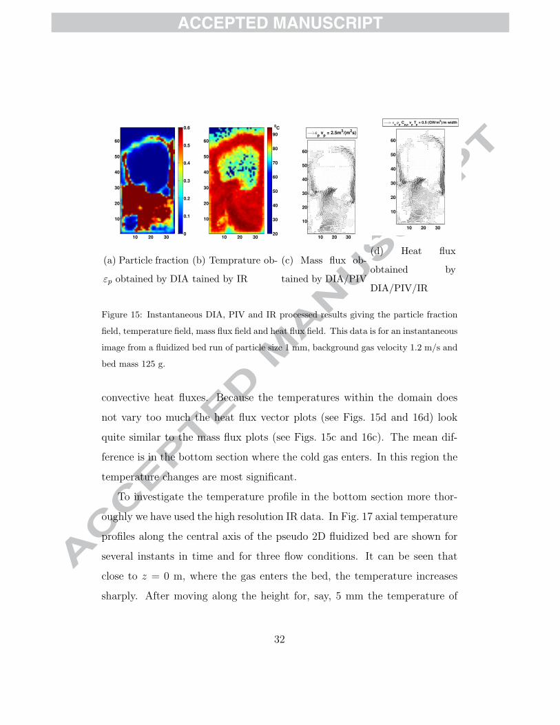
Figure 15: Instantaneous DIA, PIV and IR processed results giving the particle fraction
field, temperature field, mass flux field and heat flux field. This data is for an instantaneous
image from a fluidized bed run of particle size 1 mm, background gas velocity 1.2 m/s and
bed mass 125 g.
convective heat fluxes. Because the temperatures within the domain does
not vary too much the heat flux vector plots (see Figs. 15d and 16d) look
quite similar to the mass flux plots (see Figs. 15c and 16c). The mean dif-
ference is in the bottom section where the cold gas enters. In this region the
temperature changes are most significant.
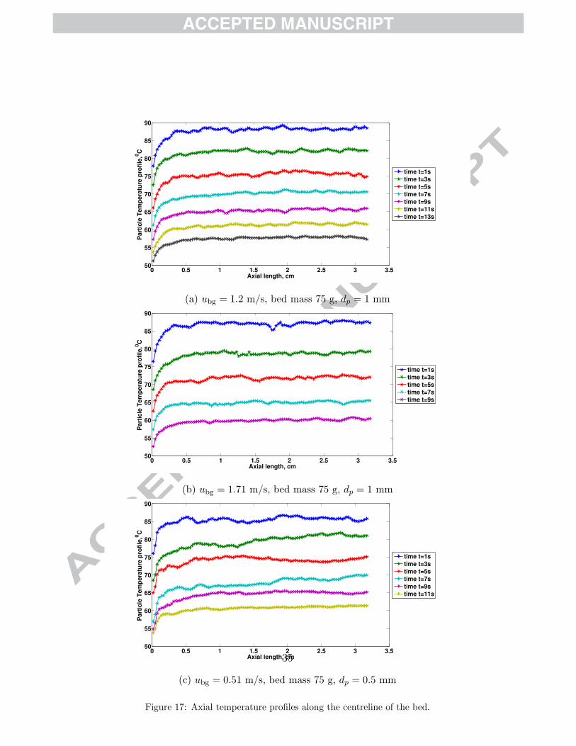
To investigate the temperature profile in the bottom section more thor-
oughly we have used the high resolution IR data. In Fig. 17 axial temperature
profiles along the central axis of the pseudo 2D fluidized bed are shown for
several instants in time and for three flow conditions. It can be seen that
close to z = 0 m, where the gas enters the bed, the temperature increases
sharply. After moving along the height for, say, 5 mm the temperature of
32
Page 34
10 20 30
10
20
30
40
50
60
0
0.1
0.2
0.3
0.4
0.5
0.6
(a) Particle fraction
εp obtained by DIA
0C
10 20 30
10
20
30
40
50
60
20
30
40
50
60
70
(b) Temprature ob-
tained by IR
10 20 30
10
20
30
40
50
60
εp v
p = 2.5m
3/(m
2s)
(c) Mass flux ob-
tained by DIA/PIV
10 20 30
10
20
30
40
50
60
εs ρ
p C
p,p v
p T
p = 0.5 (GW/m
2)/m depth
(d) Heat flux
obtained by
DIA/PIV/IR
Figure 16: Instantaneous DIA, PIV and IR processed results giving the particle fraction
field, temperature field, mass flux field and heat flux field. This data is for an instantaneous
image from a fluidized bed run of particle size 1 mm, background gas velocity 1.2 m/s and
bed mass 75 g.
33
Page 35
the bed remains constant with only minor variation.
It is observed from these plots that at higher mean temperatures of the
bed the temperature profile increases more sharply at the inlet. As the
background gas velocity increases the temperature gradient at the inlet also
increases. This is expected because the heat transfer coefficient increases
as the gas velocity increases. By comparing Fig. 17c, which shows 0.5 mm
particle data, with plots 17a-b, which show 1 mm data, it is seen that the
temperature profile at the inlet is sharper for the smaller particle size. As
0.5 mm particles are smaller they have a larger specific area causing a higher
bed heat transfer coefficient even for background velocities that are smaller
than in case of the 1 mm particles.
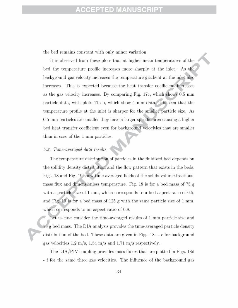
5.2. Time-averaged data results
The temperature distribution of particles in the fluidized bed depends on
the solidity density distribution and the flow pattern that exists in the beds.
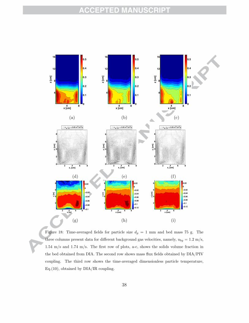
Figs. 18 and Fig. 19 show time-averaged fields of the solids-volume fractions,
mass flux and dimensionless temperature. Fig. 18 is for a bed mass of 75 g
with a particle size of 1 mm, which corresponds to a bed aspect ratio of 0.5,
and Fig. 19 is for a bed mass of 125 g with the same particle size of 1 mm,
which corresponds to an aspect ratio of 0.8.
Let us first consider the time-averaged results of 1 mm particle size and
75 g bed mass. The DIA analysis provides the time-averaged particle density
distribution of the bed. These data are given in Figs. 18a - c for background
gas velocities 1.2 m/s, 1.54 m/s and 1.71 m/s respectively.
The DIA/PIV coupling provides mass fluxes that are plotted in Figs. 18d
- f for the same three gas velocities. The influence of the background gas
34
Page 36
0 0.5 1 1.5 2 2.5 3 3.550
55
60
65
70
75
80
85
90
Axial length, cm
Parti
cle
Tem
peratu
re p
ro
file
, 0C
time t=1s
time t=3s
time t=5s
time t=7s
time t=9s
time t=11s
time t=13s
(a) ubg = 1.2 m/s, bed mass 75 g, dp = 1 mm
0 0.5 1 1.5 2 2.5 3 3.550
55
60
65
70
75
80
85
90
Axial length, cm
Parti
cle
Tem
peratu
re p
ro
file
, 0C
time t=1s
time t=3s
time t=5s
time t=7s
time t=9s
(b) ubg = 1.71 m/s, bed mass 75 g, dp = 1 mm
0 0.5 1 1.5 2 2.5 3 3.550
55
60
65
70
75
80
85
90
Axial length, cm
Parti
cle
Tem
peratu
re p
ro
file
, 0C
time t=1s
time t=3s
time t=5s
time t=7s
time t=9s
time t=11s
(c) ubg = 0.51 m/s, bed mass 75 g, dp = 0.5 mm
Figure 17: Axial temperature profiles along the centreline of the bed.
35
Page 37
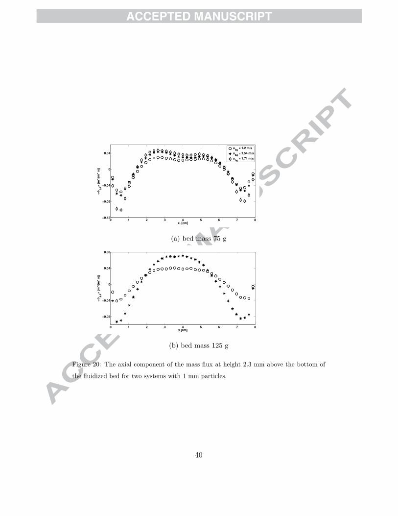
velocity is noticeable in the circulation pattern of the particulate phase. The
increase in the background gas velocity causes a more pronounced circulation
and back mixing of particles in the bed. This can be observed more closely in
the Fig. 20a that shows the cross-sectional profile of the mass flux for these
three background gas velocities at a height of 2.3 mm above the bottom plate.
A typical instantaneous IR image was shown earlier in Fig. 2. Here one
sees a small jet of cold particles issuing into the bed from the bottom-centre
of the bed. This is a typical narrow cold zone created along the axial direction
from the bottom that tends to diminish as it propagates into the bed. This
narrow cold zone (‘jet’) of particles is created due to the circulation pattern
of the particles which moves from the sides of the bed to centre from the
bottom. During this process the particles come into contact with fresh cold
gas and exchange more heat before moving upward from the centre. During
fluidization runs, the jet oscillates in the bed with a relatively stable base.
It was observed that at the lower background gas velocity of 1.2 m/s the
narrow cold zone is more stable compared to higher background gas velocity.
Thus when a time-average of the dimensionless temperature distribution is
computed, using Eq. (10), we obtain a distribution as shown in Fig. 18g. In
this figure at the centre bottom the narrow cold zone leaves its mark. This
causes relatively hotter zones to appear on the sides of the bed.
At higher background gas velocities the narrow cold zone tends to oscillate
more as well as move around the bottom of the bed. Thus when a time-
averaging is performed the resulting field is more uniform. This can be
observed for background gas velocities 1.54 and 1.71 m/s in Fig. 18h and
Fig. 18i, respectively. Also the hotter zones forming at the sides of the
36
Page 38
pseudo 2D bed tend to diminish at higher background gas velocity.
Now let us consider and analyse the distribution profiles for higher bed
mass of 125 g and bed aspect ratio of 0.8 with the same particle size of 1 mm.
Here background gas velocities of 1.2 m/s and 1.54 m/s are considered for
which various plots and profiles are shown in Fig. 19. The time-averaged
particle fraction data are shown in Figs. 19a-b for runs at background gas
velocities of 1.2 m/s and 1.54 m/s respectively. Following this the mass flux
profile giving the flow pattern is shown in Figs. 19c-d. The axial component
of the mass flux at a bed height of 2.3 mm is shown in Fig. 20b. Here it
can be seen that, as the background gas velocity increases from 1.2 m/s to
1.54 m/s, the mass flux also increase causing greater circulation of particles.
The narrow cold zone created in the 75 g bed for background gas velocty
1.2 m/s is not that pronounced in the system with bed mass 125 g. Therefore
the hot zone tend to stay in the centre as shown in Fig. 19e. However, for the
higher background gas velocity of 1.54 m/s the hot zone formation is again
towards to the sides with cold zones forming at the centre bottom. This
indicate that the narrow cold zone forming at the bottom is affected by the
bed aspect ratio as well.
5.3. Position averaged data results
The DIA/IR image processing detailed in the section 4.2 was applied to
all the fluidized bed runs listed in Table 1. By means of these procedures the
mean particle temperature was calculated as function of time and plotted
together for comparison. Fig. 21 shows a plot of the mean particle tempera-
ture change with respect to time for the bed mass of 75 g and particle sizes
1 mm and 0.5 mm. There are two important observations that can be made
37
Page 39
x [cm]
z [
cm
]
4 8
4
8
12
16
0
0.1
0.2
0.3
0.4
0.5
(a)
x [cm]
z [
cm
]
4 8
4
8
12
16
0
0.1
0.2
0.3
0.4
0.5
(b)
x [cm]
z [
cm
]
4 8
4
8
12
16
0
0.1
0.2
0.3
0.4
0.5
(c)
2 4 6 80
2
4
6
8
x, [cm]
z, [c
m]
<εp v
p> = 0.05 m
3/(m
2s)
(d)
2 4 6 80
2
4
6
8
x, [cm]
z, [c
m]
<εp v
p> = 0.05 m
3/(m
2s)
(e)
2 4 6 80
2
4
6
8
x, [cm]
z, [c
m]
<εp v
p> = 0.05 m
3/(m
2s)
(f)
x [m]
z [
m]
2 4 6 8
2
4
6
8
−0.1
−0.08
−0.06
−0.04
−0.02
0
0.02
0.04
(g)
x [cm]
z [
cm
]
2 4 6 8
2
4
6
8
−0.12
−0.1
−0.08
−0.06
−0.04
−0.02
0
0.02
(h)
x [cm]
z [
cm
]
2 4 6
2
4
6
8
−0.12
−0.1
−0.08
−0.06
−0.04
−0.02
0
0.02
(i)
Figure 18: Time-averaged fields for particle size dp = 1 mm and bed mass 75 g. The
three columns present data for different background gas velocities, namely, ubg = 1.2 m/s,
1.54 m/s and 1.74 m/s. The first row of plots, a-c, shows the solids volume fraction in
the bed obtained from DIA. The second row shows mass flux fields obtained by DIA/PIV
coupling. The third row shows the time-averaged dimensionless particle temperature,
Eq.(10), obtained by DIA/IR coupling.
38
Page 40
x [cm]
z [
cm
]
4 8
4
8
12
16
0.1
0.2
0.3
0.4
0.5
(a)
x [cm]
z [
cm
]
4 8
4
8
12
16
0.1
0.2
0.3
0.4
0.5
(b)
4 8
4
8
12
x [cm]
z [
cm
]
<εp v
p> = 0.05 m
3/(m
2s)
(c)
4 8
4
8
12
x [cm]
z [
cm
]
<εp v
p> = 0.05 m
3/(m
2s)
(d)
x [cm]
z [
cm
]
4 8
4
8
12
−0.1
−0.08
−0.06
−0.04
−0.02
0
0.02
0.04
(e)
x [cm]
z [
cm
]
4 8
4
8
12
−0.1
−0.08
−0.06
−0.04
−0.02
0
0.02
0.04
(f)
Figure 19: Time-averaged fields for particle size dp = 1 mm and bed mass 125 g. The
two columns present data for different background gas velocities, namely, ubg = 1.2 m/s
and 1.54 m/s. The first row of plots shows the solids volume fraction in the bed obtained
from DIA. The second row shows mass flux fields obtained by DIA/PIV coupling. The
third row shows the time-averaged dimensionless particle temperature, Eq.(10), obtained
by DIA/IR coupling.
39
Page 41
0 1 2 3 4 5 6 7 8−0.12
−0.08
−0.04
0
0.04
x, [cm]
<Φ
p,z
> [
m3/(
m2 s
)]
ubg
= 1.2 m/s
ubg
= 1.54 m/s
ubg
= 1.71 m/s
(a) bed mass 75 g
0 1 2 3 4 5 6 7 8
−0.08
−0.04
0
0.04
0.08
x [cm]
<Φ
p,z
> [
m3/(
m2 s
)]
(b) bed mass 125 g
Figure 20: The axial component of the mass flux at height 2.3 mm above the bottom of
the fluidized bed for two systems with 1 mm particles.
40
Page 42
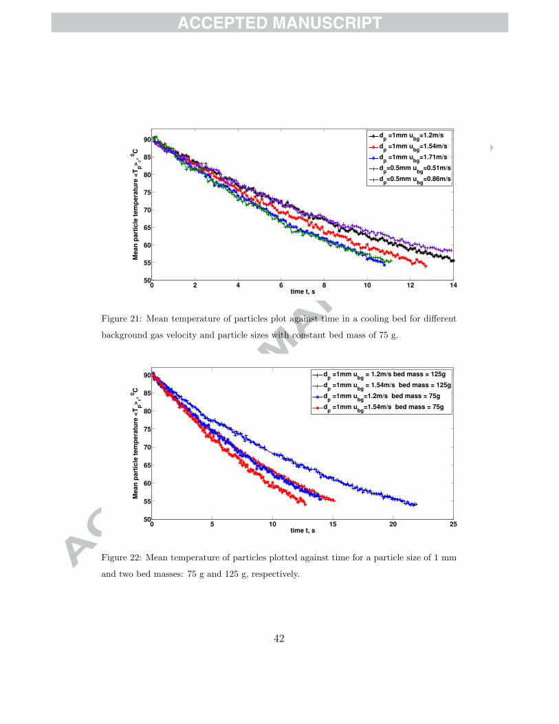
from this plot. For one particle size of 1 mm or 0.5 mm, as the background
gas velocity is increased the cooling rate of the bed also increases. Further-
more, as the particle size decreases the cooling rate of the bed increases.
The background gas velocity for 1 mm particle are 1.2 m/s, 1.54 m/s and
1.71 m/s which are 2.06, 2.66 and 2.95 times minimum fluidization velocity
(umf = 0.58 m/s). Similarly, the background gas velocity for 0.5 mm parti-
cles is 0.51 m/s and 0.86 m/s, which are 2.83 and 4.78 times the minimum
fluidization velocity (umf = 0.18 m/s).
All curves in Fig. 21 are for the same bed mass of 75 g. In Fig. 22 we
present a comparison between the cooling rate for two bed masses, namely,
75 g and 125 g with otherwise the same 1 mm particle size and two back-
ground velocities. The higher bed mass gives a slower rate of cooling of the
bed as expected.
These plots accurately give the rate of heat loss of the particles. This heat
loss is the sum of heat exchange between particles and gas due to multiphase
flow, heat radiating from the particles to the surrounding and heat exchange
between the gas phase and surrounding walls by means of heat conduction.
In this paper we do not try to quantify these quantities but using DEM some
of these heat exchange types have been quantified in the literature [5, 6].
Using some direct measurements shown in this work these quantities can
be validated. The plot in Fig. 22 can quantify gas particle convective heat
transfer as it is a plot for the same particle size and background gas velocity
but different bed mass. As the gas flowing through the particles becomes
thermally saturated the remaining heat will be lost due to other transfer
mechanisms like radiation.
41
Page 43
0 2 4 6 8 10 12 1450
55
60
65
70
75
80
85
90
time t, s
Mean
parti
cle
tem
peratu
re <
Tp>
ε,
0C
dp =1mm u
bg=1.2m/s
dp =1mm u
bg=1.54m/s
dp =1mm u
bg=1.71m/s
dp=0.5mm u
bg=0.51m/s
dp=0.5mm u
bg=0.86m/s
Figure 21: Mean temperature of particles plot against time in a cooling bed for different
background gas velocity and particle sizes with constant bed mass of 75 g.
0 5 10 15 20 2550
55
60
65
70
75
80
85
90
time t, s
Mean
parti
cle
tem
peratu
re <
Tp>
ε,
0C
dp =1mm u
bg = 1.2m/s bed mass = 125g
dp =1mm u
bg = 1.54m/s bed mass = 125g
dp =1mm u
bg=1.2m/s bed mass = 75g
dp =1mm u
bg=1.54m/s bed mass = 75g
Figure 22: Mean temperature of particles plotted against time for a particle size of 1 mm
and two bed masses: 75 g and 125 g, respectively.
42
Page 44
6. Conclusion
A measuring technique involving the use of visual and infrared images has
been developed. The visual and IR recordings were successfully synchronized
and combined by a high resolution image mapping. The mean temperature of
particles in the bed was calculated with respect to time for different particle
sizes, background gas velocity and bed mass (aspect ratio). With these plots
the varying exchange rate between particles and gas can be calculated. Time
averaged temperature distribution fields of the fluidised bed were calculated
and presented for various configurations. They were compared and analysed
with their respective particle volume fraction and also mass and heat flux
data was computed.
With this work processed measurements of four important synchronized
parameters of multiphase flow in non-isothermal pseudo 2D fluidized beds
are made available, namely, solids volume fractions, temperature fields and
mass- and heat-flux fields. This has produced a data sets that can be used to
analyze the heat transfer mechanisms inside a fluidized bed in more detail,
e.g., by comparison with CFD computations.
Notation
dp Particle diameter, m
ubg Background or fluidization velocity, m/s
umf Minimum fluidization velocity, m/s
vp Time average particle velocity, m/s
43
Page 45
ΦΦΦp Time averaged particulate mass flux, m3/m2s
ρp Particle density, kg/m3
σp Standard deviation of particle temperature distribution, K
εp Particle density fraction 3D
ε2D Particle density fraction 2D
ε3D Particle density fraction 3D
A Fitting parameter
B Fitting parameter
Cp,p Particle heat capacity, J/kg K
Tp Particle temperature, K
Hp Particulate heat flux, (GW/m2)/m width
Acknowledgments
The authors would like to thank the European Research Council for its
financial support, under its Advanced Investigator Grant scheme, contract
number 247298 (Multiscale Flows). This research was also supported by
the Dutch Technology Foundation STW, applied science division of NWO
and the Technology Program of the Ministry of Economic Affairs in The
Netherlands. The authors would also like to acknowledge the Dutch polymer
institute (DPI) which had supported the building of the set up. The tech-
nicians Lee McAlpine and Paul Aendenroomer (TNO) are specially thanked
44
Page 46
for constructing and maintaining the set up. The author would also like to
thank T.Y.N. Dang, S. Shirsath and Y.M. Lau for helping out with image
processing. Acknowledgment also goes to Mariet Slagter, Stijn Smits, Tom
Kolkman and Rohit Rewagad for providing help and suggestions at various
stages during the development of the set up and measurement method.
References
[1] J. Davidson, D. Harrison, Fluidised Particles, Cambridge University
Press, 1963.
[2] D. Kunii, O. Levenspiel, Fluidization engineering, Butterworth-
Heinemann series in chemical engineering, Butterworth-Heinemann
Limited, 1991.
[3] D. Gunn, Transfer of heat or mass to particles in fixed and fluidised
beds, Int. J. Heat and Mass Transfer 21 (1978) 467–476.
[4] V. Ganzha, S. Upadhyay, S. Saxena, A mechanistic theory for heat
transfer between fluidized beds of large particles and immersed surfaces,
International Journal of Heat and Mass Transfer 25 (1982) 1531 – 1540.
[5] Z. Y. Zhou, A. B. Yu, P. Zulli, Particle scale study of heat transfer in
packed and bubbling fluidized beds, AIChE Journal 55 (2009) 868–884.
[6] Z. Zhou, A. Yu, P. Zulli, A new computational method for studying heat
transfer in fluid bed reactors, Powder technology 197 (2010) 102–110.
45
Page 47
[7] P. Basu, P. Nag, An investigation into heat transfer in circulating flu-
idized beds, International Journal of Heat and Mass Transfer 30 (1987)
2399 – 2409.
[8] C. Heerden, A. Nobel, D. Krevelen, Mechanism of heat transfer in
fluidized beds, Industrial and Engineering Chemistry 45 (1953) 1237–
1242.
[9] V. Borodulya, V. Ganzha, Y. Teplitskii, Y. Epanov, Heat transfer in
fluidized beds, Journal of engineering physics 49 (1985) 1197–1202.
[10] J. Valenzuela, L. Glicksman, An experimental study of solids mixing in
a freely bubbling two-dimensional fluidized bed, Powder Technology 38
(1984) 63 – 72.
[11] T. Tsuji, T. Miyauchi, S. Oh, T. Tanaka, Simultaneous measurement of
particle motion and temperature in two-dimensional fluidized bed with
heat transfer, Kona Powder and Particle Journal (2010) 167–179.
[12] S. L. Brown, B. Y. Lattimer, Transient gas-to-particle heat transfer mea-
surements in a spouted bed, Experimental Thermal and Fluid Science
44 (2013) 883 – 892.
[13] P. Findlay, G. R. Peck, K. R. Morris, Determination of fluidized bed
granulation end point using near-infrared spectroscopy and phenomeno-
logical analysis, J. Pharm. Sci. 94 (2005) 604–612.
[14] T. Astarita, G. Carlomagno, Infrared Thermography for Thermo-Fluid-
Dynamics, Experimental fluid mechanics, Springer, 2012.
46
Page 48
[15] M. Vollmer, K. Mollmann, Infrared Thermal Imaging: Fundamentals,
Research and Applications, Wiley, 2011.
[16] H. Kaplan, Practical Applications of Infrared Thermal Sensing and
Imaging Equipment, Tutorial Text Series, Society of Photo Optical,
2007.
[17] T. Dang, T. Kolkman, F. Gallucci, M. van Sint Annaland, Development
of a novel infrared technique for instantaneous, whole-field, non invasive
gas concentration measurements in gas-solid fluidized beds, Chemical
Engineering Journal 219 (2013) 545 – 557.
[18] M. S. van Buijtenen, M. Borner, N. G. Deen, S. Heinrich, S. Antonyuk,
J. Kuipers, An experimental study of the effect of collision properties
on spout fluidized bed dynamics, Powder Technology 206 (2011) 139 –
148.
[19] J. de Jong, S. Odu, M. van Buijtenen, N. Deen, M. van Sint Annaland,
J. Kuipers, Development and validation of a novel digital image analysis
method for fluidized bed particle image velocimetry, Powder Technology
230 (2012) 193 – 202.
[20] D. DeWitt, G. Nutter, Theory and Practice of Radiation Thermometry,
Wiley-interscience publication, Wiley, 1988.
[21] M. Modest, Radiative Heat Transfer, Elsevier Science, 2003.
47
Page 49
• Heat transfer in a fluidized beds is studied experimentally
• New measurement technique proposed: coupling IR with DIA and PIV
• Calibration of the infrared measuring technique is discussed
• Post-processed the temperature distributions as well as mass and heat fluxes are
analyzed