Air Force Institute of Technology Air Force Institute of Technology AFIT Scholar AFIT Scholar Theses and Dissertations Student Graduate Works 3-2000 A Study of Morning Radiation Fog Formation A Study of Morning Radiation Fog Formation Jimmie L. Trigg Jr. Follow this and additional works at: https://scholar.afit.edu/etd Part of the Meteorology Commons Recommended Citation Recommended Citation Trigg, Jimmie L. Jr., "A Study of Morning Radiation Fog Formation" (2000). Theses and Dissertations. 4872. https://scholar.afit.edu/etd/4872 This Thesis is brought to you for free and open access by the Student Graduate Works at AFIT Scholar. It has been accepted for inclusion in Theses and Dissertations by an authorized administrator of AFIT Scholar. For more information, please contact richard.mansfield@afit.edu.
Transcript
Air Force Institute of Technology Air Force Institute of Technology
AFIT Scholar AFIT Scholar
Theses and Dissertations Student Graduate Works
3-2000
A Study of Morning Radiation Fog Formation A Study of Morning Radiation Fog Formation
Jimmie L. Trigg Jr.
Follow this and additional works at: https://scholar.afit.edu/etd
Part of the Meteorology Commons
Recommended Citation Recommended Citation Trigg, Jimmie L. Jr., "A Study of Morning Radiation Fog Formation" (2000). Theses and Dissertations. 4872. https://scholar.afit.edu/etd/4872
This Thesis is brought to you for free and open access by the Student Graduate Works at AFIT Scholar. It has been accepted for inclusion in Theses and Dissertations by an authorized administrator of AFIT Scholar. For more information, please contact [email protected].
DDL Interactive Development Language (computer programming language)
LCL Lowest Condensation Level
MIFG Visibility obscuration entry indicating shallow patchy ground fog
NONE Visibility obscuration entry indicating no obstruction to visibility is
Observed
PLCL Pressure of the LCL
P Atmospheric pressure
R Universal Gas Constant (8.3143*10A3 J deg"1 Kmol"1)
r2 Coefficient of Determination (1 - (SSE / SST))
SSE Error Sum of Squares (SSE = Z(YAj - Y;)2)
SST Total Sum of Squares (SST = S(Yj - Ybar;)2)
Tbar Average Temperature Between Two Pressure Levels
T Temperature
TLCL Temperature of the LCL
ZLCL Height of the LCL
UTC Greenwich Mean Time
p Density
Abstract
This research focuses on developing a linear regression formula that forecasters in
the Midwest can use to accurately anticipate the formation of radiation fog. This was
accomplished in three stages. First a study of the surface and upper air parameters and
processes required to develop radiation fog were identified and explored. Next, a linear
regression technique was applied to the 23 parameters identified. The top four indicators
were then reprocessed and a new linear regression equation was developed. Finally, the
new regression equation was compared to an existing fog forecasting technique. The
existing forecast technique selected was the 2nd Weather Wings "Fog Stability Index."
Hit rates, False Alarm Rates and Threat Scores for both methods were calculated and
compared. In general the linear regression, while only accounting for 45 to 50 percent of
the total error (SST), outperformed the Fog Stability Index in ability to accurately
forecast the development of radiation fog, and greatly reduced the number of incorrect
forecasts. The new linear regression equation reduced the false alarm rate on fog
forecasting by 23 to 43 percent and increased the threat score ability 30 to 60 percentage
points.
Vlll
A STUDY OF MORNING RADIATION FOG FORMATION
1. Background and Statement of the Problem
1.1. Background
Accurately forecasting radiation fog is a significant problem at many weather
stations. "From a meteorological point of view, fog occurrence and severity are hard to
predict, and only those forecasters with a good understanding of the local climatology
and meteorology are able to demonstrate fog forecasting skill" (Lala 1987). This
statement is seen in numerous reviews of missed fog forecasts through the years. The
major difficulty in forecasting fog is that similar synoptic conditions that produced fog
one morning may not produce fog the next (Lala 1987).
Forecasters usually have all the data they need to forecast the formation of
radiation fog accurately, but fail to apply these tools correctly. There has been a great
deal of literature written by the Air Force, civilian forecasters, and academic researchers
on how fog forms. This literature, unfortunately, has not been effectively crossed to the
forecasters.
1.2 Statement of the Problem
Leaders in Weather Stations need a "toolbox" filled with meteorological
principles that are grounded in scientific reason and research. Once the governing
physical principles of radiation fog formation are fully understood, forecasters can be
guided, using the 'Tunneling Technique," into correctly forecasting the onset and
duration of radiation fog. By researching fog formation, centering on tools already
accessible to forecasters, and cross feeding this information, weather personnel may be
able to improve their overall success rate in forecasting fog that can limit operations.
1.3. Organization
Chapter 2 examines the fundamental processes that contribute to fog formation.
In this chapter, each process is defined and explained as to its impact on the development
and continuation of radiation fog. In addition, elements readily accessible to the counter
forecaster that indicate these processes in motion are noted. Past rules of thumb and
simple numerical prediction methods are also listed.
Chapter 3 goes into depth concerning the data required for this research. It covers
the data sources, manipulation techniques, computer programs, and filtering schemes
employed. The author discusses how missing data was interpolated and how verification
data was separated from the main data set.
Results and conclusions are discussed in Chapter 4. Here the regression formula
and its verification results are compared to an existing forecasting fog technique.
Finally, Chapter 5 discusses future research opportunities and recommendations
for improving the radiation fog formation forecasting skill for Air Force Weather
personnel.
2. Radiation Fog Formation Causes and Processes
2.1. Basics Definitions
Ahrens (1988) defines fog as a cloud with its base at the Earth's surface reducing
horizontal visibility to less than 1 km. Since fog is defined as a cloud, it stands to reason
that it will follow the same "rules" as clouds during formation, dissipation, and advection.
Meteorologists categorize clouds based on their height and structure; so too, fog is
divided into four basic types based on its formation process. The four major types of fog
are evaporation, upslope, advection, and radiation (Ahrens 1988). The simplest example
of evaporation fog is the cloud you see when you exhale outside on a cold day. The
warm moisture from your breath saturates the colder air outside causing fog (Ahrens
1988). Upslope fog, as its name implies, forms as air is forced vertically by orographic
features. From the ideal gas law, P=pRT, air that is forced upward to a lower pressure
must cool (Holton 1992). In the equation above, P is the pressure, p is the density, T is
the temperature of the air parcel and R is the Universal Gas Constant. If this air cools to
the dew point, fog forms. In advection fog, the temperature of the parcel decreases or the
moisture content increases based on its path and its interaction with the surrounding
environment (Ahrens 1988). As air moves into cooler areas, its temperature drops until it
is in thermal equilibrium with its surrounding environment. Similarly, an airmass that
passes over a moisture source increases its relative humidity until it reaches saturation.
Fog forms when this cooling reaches the dew point. Radiation fog forms very similarly
to upslope and advection fog; however, radiation fog usually develops, intensifies, and
dissipates in a relatively confined area. The air mass cools, not from advection or ascent,
but through radiative transfer. This particular type of fog is the most difficult for
forecasters to predict accurately as it initially forms in a very small area and rapidly
increases or disappears with apparent randomness.
2.2 Causes
The key processes that produce radiation fog are mixing of different air masses,
radiative cooling, rapidly falling pressure, scattering of visible light, adjusting the
moisture content of the air mass, and temperature differentials (Fleagle and Businger
1980). The Air Force has reduced this list to two simple processes: increasing the
moisture, or decreasing the temperature (AFWA 1998). Forecasters must remember that
fog forms not from one particular cause, but from a combination of events (AFWA
1998). "As fog occurs within the boundary layer, a forecaster must focus on the
evolution of weather across all scales that may lead to saturation of all or some portion of
the boundary layer." (Croft et al. 1997)
a. Mixing
Mixing of adjacent air masses is a major cause of radiation fog. Forecasters must
understand the basic principles behind mixing to understand how this process affects fog
formation. According to Iribarne and Cho (1980), "If two different adjacent air masses
mix, the process occurs essentially at constant pressure," and if there is no condensation,
the properties of the resulting mixture will be a mass weighted average of the original
parameters. Dew point does not follow this rule. The final dew point for a mixture will
be higher than the corresponding linear average of the individual dew points due to the
exponential form of the Clausius-Clapeyron equation (Fleagle and Businger 1980). By
recalling that the log differential of the specific humidity, and thus the dew point, is equal
to the log differential of the saturation vapor pressure, the Clausius-Clapeyron equation in
its empirical, standard atmospheric form reduces to
logl0(es)=11.40 - 2353/T
where es is the saturation vapor pressure and T is the temperature of the airmass (Fleagle
and Businger 1980). This equation shows vapor pressure of a gas is not a linear function
of the temperature of the gas.
According to Iribarne and Cho (1980), a mixture can be represented on a plot of vapor
pressure vs. temperature as a point on a line between the initial parameters. However,
this can lead to supersaturation of the mixture as illustrated in Figure 2.1. When this
occurs, the water vapor in the gas will condense until the mixture reaches the saturation
vapor pressure curve.
Forecasters can easily calculate a resulting temperature either from the equation above
or by interpolating the graph below. This illustrates that mixing of the atmosphere can
result in supersaturation of the lowest levels of the atmosphere, thus contributing to fog
formation. It is important to note that although some turbulence is required for the
atmosphere to mix and reach saturation or supersaturation values, too much mixing can
entrain drier air from aloft into the mixture thus greatly reducing the moisture content. In
general, winds speeds less then 2-3 knots will not mix enough of the atmosphere, where
winds speeds in excess of 7 knots will entrain dry air (WPAFB LAFP 1999).
Figure 2.1. Vapor Pressure Vs Temperature. Points A and B indicate the initial conditions. Point C is the mass weighted average temperature and vapor pressure. The air mass at C is supersaturated and must follow the line down to the saturation vapor pressure curve. (Iribarne and Cho 1980)
b. Radiative Cooling
Radiative cooling is another contributing factor to the formation of radiation fog.
Radiative cooling is best explained as a system of energy balance equations. Fleagle and
Businger (1980) use a parcel of air over a cooling surface to illustrate how the air cools
through radiative exchanges. If we assume the air and surface temperature profiles are
continuous, the boundary between the air and surface has a given temperature. We also
assume that the air in a shallow layer is isothermal. Finally, we also assume that the
ground is cooling due to longwave radiation, and that longwave radiation is passing
through the airmass without being absorbed. With these assumptions we can create a
system of balancing equations. As the ground cools, energy in the form of heat is
transferred from the air just above the ground to the ground. This exchange results in a
cooling of the air in the layer just above the ground. As this layer continues to transfer
energy to the ground, and thus cool, the air above this layer, which is now relatively
warmer, begins to transfer energy into the lower layer, slowing that layers temperature
drop. The temperature in the lowest level continues to drop until it reaches either
saturation or thermal equilibrium. At this point there may exist a portion of this lower
layer where the net exchange in energies going to the ground and coming from the layer
above, are balanced and there is no net increase or decrease in temperature (Fleagle and
Businger 1980). This forms a temperature inversion where the change in temperature
with height equals 0.0.
Height
Ground
Original Temperature Profile
Resulting Temperature Profile
\ /" /
/ /
Temperature Inversion
<f
Temperature Figure 2.2. Cooling of the Near Surface Airmass. Resulting temperature profile indicates a temperature inversion has formed at the point where the change in temperature with height equals 0.0
Close examination of the evening sounding can give the forecaster a warning that
this process is likely to occur. Carefully estimating the amount of warm air advection
and taking into account the amount of solar energy imparted to the ground during the day
can aid the forecaster in deciding if adequate energy transfer can occur.
c. Rapidly Falling Pressure
An easier and quicker way to create fog is to lower the atmospheric pressure rapidly.
Bohren (1987) noted that the air trapped above a carbonated liquid in a bottle is usually
twice the sea level pressure of the air outside the bottle. "When the bottle is uncapped,
this gas escapes rapidly from the neck and its pressure drops greatly" (Bohren 1987).
From the ideal gas law we know that P=pRT. When the pressure drops, the temperature
and density must change. Since the drop is sudden, the density, and thus the water vapor
present in the air, does not have time to decrease. Instead, the temperature drops rapidly
to keep pace with the pressure. Consequently, the temperature reaches supersaturation
values, and the moisture condenses in the neck of the bottle creating fog.
Although such a drastic event may not appear to be practical in the real atmosphere,
rapidly dropping pressures can be a contributing factor to fog formation. The forecaster
must recall that fog is not caused by a single event but by a combination of supporting
processes. Although pressure drops of a magnitude required to reach saturation are
seldom witnessed in the environment, the remark "pressure falling rapidly" in the
observation may indicate a sympathetic or supporting process is occurring.
d. Scattering
Scattering is the reason fog is a hindrance to operations. The amount of water vapor
in the air does not reduce visibility. Wallace and Hobbs (1977) noted that fog has a
relatively uniform structure over a large horizontal scale, with a liquid water content
generally only a few tenths of a gram per cubic meter. Visibility is reduced however,
because light interacts with suspended particles. Human eyes are sensitive to a narrow
band of radiation in the 0.4 to 0.7 micrometer wavelength known as visible light (Ahrens
1988). Scattering is dependent on the size of the molecule relative to the wavelength of
the incident radiation. Fog droplets have an average size of 20.0 micrometer and thus
result in near geometric scattering (Schanda 1986). With this scattering, the light from
distant objects is refracted in all directions, greatly reducing the amount of light reaching
the observer, thus reducing visibility. The initial size of the condensation nuclei plays an
important role in how much condensation must accumulate on the particle for it to begin
restricting visibility. According to Ahrens (1988), condensation can begin with relative
humidities as low as 75%. Therefore, fog can form and restrict visibility even before the
temperature reaches the dew point.
In this case, observers play a vital role in forecasting fog formation. A thin haze layer
or a slight restriction to visibility in the lowest levels can indicate the presence of
condensation nuclei in the atmosphere. Since the visibility is already beginning impaired
by the size of these nuclei, it takes a relatively small amount of water vapor condensing
on these particles to restrict visibility severely,
e. Moisture
The processes mentioned in the above sections, mixing, radiative cooling, rapidly
falling pressure, and scattering all require one common factor to be effective, moisture.
Without moisture, there is no condensation at any temperature. Moisture is introduced
into an airmass in several ways; precipitation, evaporation from wet surfaces, and
moisture advection are the most common (AFWA 1998).
As rain falls through the atmosphere, it evaporates and thus increases the dew point of
the air mass. Once the precipitation has ended, puddles will slowly evaporate adding
moisture to the air. Even if there was no precipitation or standing water in the general
area, advection can infuse moisture into the airmass.
Advection of moisture can occur by bringing air in from an area that has had
precipitation, or by bringing in air that is warmer and has more suspended water vapor.
Wind speed and direction are also very important in this respect. Strong winds can cause
excessive mixing and inhibit fog formation. On the other hand, air masses that bring
additional moisture into the area can be a source of fog.
Plants can also contribute moisture to the atmosphere through transpiration. Griend
and Camillio (1986) found that plants, grasses in particular, contributed greatly to the
amount of water vapor in the air. They found that grass in excess of 10 cm in length can
raise the dew point as much as 1 to 1.5 degrees Celsius during the night. In this case, the
forecaster must fully appreciate the events that have occurred to create moisture sources
at the station of interest and upstream. In addition, he has to have knowledge of the
immediate vicinity of the airfield. Items such as the relative height and condition of the
infield grass, succulent crops growing in adjacent fields, and such, are important features
to note. Coupled with a sound minimum temperature forecast, the forecaster and
observer should note the trend of the dewpoint. Continued evaporation of standing water
or advection of moisture will be evident in an increase in the dewpoint. Rapidly falling
10
temperatures and climbing dewpoint readings should indicate to the forecaster that the
potential for fog formation is rapidly increasing,
f. Temperature
Perhaps the most important fog formation parameter after moisture is temperature.
The diurnal temperature change is perhaps the single most recognized cause of fog
formation. Even the definition of fog formation, "the cooling of air below its dew point",
illustrates the importance of temperature (Wallace and Hobbs 1977). Temperature drops
can be contributed to two main causes, long wave radiation (Wallace and Hobbs 1977)
and evaporation (AFWA 1998).
During the night, solar radiation is cut off, and the earth begins to cool. Long wave
radiation is released from the earth skyward (Iribarne and Cho 1980). If there are no
clouds to absorb or reflect this radiation then the surface will cool rapidly. Once the
surface cools, the actions cited in the irradiance section become the dominant process.
The air cools until it reaches thermal equilibrium. This equilibrium point could be
saturation, in which case fog forms, or radiative transfer equilibrium where the exchange
of heat with the air and ground balance at a temperature above saturation values.
When calculating the temperature equilibrium point, forecasters often dismiss
evaporation. Condensation is the mechanism for drawing moisture from the air and
forming fog; however, evaporation can occur during the day adding moisture and through
the early part of the night cooling the air to the saturation point. Once the air cools,
added moisture through transpiration, continued evaporation of standing water, or
moisture advection can produce fog. Once dew forms, it is a common belief that fog will
not form. Forecasters must be wary of applying this rule blindly. Dew can be a ready
11
source of moisture under the right conditions. In the same way, nearby golf courses that
water during the night may be setting the stage for a major fog incident.
Diurnal temperature curves, developed by the Air Force Combat Climotology Center
in Asheville, North Carolina and delivered to every Base Weather Station in tabular
format, can assist forecasters in determining the amount of cooling to expect during the
night. These tables are specifically developed for each station and are stratified into
month, cloud cover, wind speed and wind direction. These tables give the forecaster a
good "first guess" of the expected minimum temperature (AFWA 1998).
Another method for forecasting the minimum temperature is to employ the equation
below. This equation was developed by J. M. Craddock and D. Pritchard to assist in
forecasting fog; the temperatures are in degrees Fahrenheit (AFWA 1998).
Tmin = 0.32*(Temperature at noon) + 0.55*(Dew Point at noon) + 2.12 +C
Table 2.1. Variable used in Craddock and Pritchard Equation. C is a variable dependent on the wind speed and mean cloud amount. Mean Forecast Surface Winds
Cloud Amount 0-1/8
Cloud Amount 2/8 - 3/8
Cloud Amount 4/8 - 5/8
Cloud Amount 6/8 - 8/8
<10Kt -3 -2 -1 0 >10Kt -1 0 0 +1
A critical factor when forecasting the minimum temperature is that condensation itself
can release heat into the environment. The cooling mechanism must not only be strong
enough to cool the air to the saturation point but overcome the latent heat of condensation
released. As water vapor condenses on a nucleus, it releases heat. Although for this
process the parcel is not lifted, the temperature change and heat release can be modeled
using the equation listed below (Wallace and Hobbs 1977).
- L*dws=Cp*dT + G*dz
12
Here L is the latent heat of condensation, dws is the saturation mixing ratio. Cp is the
specific heat at constant pressure for dry air. dT is the change in temperature of the
parcel. And G*dz is the force acting on a parcel as it is lifted. This equation illustrates
how as the parcel cools (dT<0) at a constant height (g*dz=0) the energy released by
condensation, in the form of heat (L*dws), is greater then zero. So as condensation
begins due to cooling, heat is released to counter the cooling. In certain circumstances,
this latent heat release may equal the effects of radiational cooling, keeping the
temperature constant. This is a very important principle that must remain foremost in the
forecaster's mind during marginal fog events.
2.3 The Five Stages of Fog Formation
Garland Lala, in his paper "Radiation Fog: Characteristics and Formation Processes"
(1987) divides the fog formation process into five distinct phases. These five phases
outline the processes that occur through the night that result in operations-inhibiting fog
at sunrise. By understanding these different stages and how each fog forming process
works within them, forecasters can better anticipate the timing and intensity of
operations-inhibiting fog.
The first phase starts at sundown. A rapid temperature drop due to radiational cooling
of the atmosphere characterizes this phase. According to Lala (1987), this cooling rate
can be as much as 2 to 3 degrees Celsius per hour. During this phase, the near adiabatic
lapse rate during the day is replaced with a strengthening temperature inversion, which
will act to isolate the low level air and moisture from the drier air aloft. It also reduces
the surface winds and the possibility of mixing. This cooling with little mixing acts to
increase the relative humidity of the surface air (Lala 1987). During this phase, observers
13
may notice a slow but steady decrease in horizontal visibility as condensation forms on
suspended hydroscopic particles.
The second phase begins two to three hours after sundown and lasts for the next eight
hours (Lala 1987). The temperature cooling rate drops to one degree Celsius per hour
and works to strengthen the inversion. Here the inversion may grow to 100 to 150 meters
from the ground while the air under the inversion is nearly saturated (Lala 1987). Short-
lived patches of fog form and move through the area. These patches could be missed at a
station with a limited meteorological watch. Close scrutiny of the Runway Visual Range
detector could be the only indicator that fog is imminent.
After about 0500 local time the mature fog stage begins (Lala 1987). The air is
saturated at the lower levels, and the maximum radiational cooling moves to the top of
the fog layer (Lala 1987). Fog begins to thicken and increase in depth as the air above
cools rapidly.
Most forecasters are familiar with the term "sunrise surprise." As the sun rises, the
top of the inversion is heated and turbulent fluxes develop. In most cases this would act
to inhibit fog formation (Lala 1987). However, in this instance it acts to intensify the fog
by thoroughly mixing the saturated air and providing even more moisture through surface
evaporation. This is the major characteristic of the fourth phase in fog development.
This phase is easily identified by the transition from a smooth surface above the fog to an
irregular boiling like texture as the fog mixes (Lala 1987).
Finally, the increased solar radiation begins to heat the surface to an extent that the
associated convective circulations mix the saturated air with the drier air aloft breaking
the inversion and dissipating the fog (Lala 1987). This phase can happen rapidly based
14
on the amount of incoming radiation and mixing. Direct absorption of solar radiation by
the atmosphere can play a role in fog dissipation, but the increased mixing due to
convection often overwhelms its effects (Lala 1987).
2.4 Fog Forecasting Techniques
A quick review of any weather station's forecast review binder will list nearly as
many ways to forecast fog as there are forecasters. Some "rules of thumb" work well,
and some are happenstance. Those based, even if unknowingly, on the physical
principles of fog formation are the most reliable. To anticipate radiation fog accurately,
the forecaster must understand the stability of the atmosphere, calculate the minimum
temperature for the night and the corresponding dew point, factor in the wind speed and
direction, and be familiar with moisture sources in the area and upstream.
a. Rules of Thumb
Fog formation is a fine line between mixing and stratification of two air masses. One
of TSgt Ritchie's, Senior Forecaster at Wright-Patterson AFB (Ritchie 1996), favorite
"rules of thumb" was that fog is unlikely if the lights of the near by city are "twinkling".
At first, this may seem insignificant, but this rule does have scientific merit. The
"twinkling" of the lights indicates the index of refraction for the air is changing. Much
like a shimmering mirage in the desert, it's indicative of vertical motion, which will mix
the low level moisture with drier air aloft inhibiting fog formation.
b. Simple Numerical Predictors
Very similarly, Herr Strauss, from the 2nd Weather Wing, USAF developed the "Fog
Stability Index" based on the difference between the 850 mb and surface parameters
(AWS 1990).
15
FI = 4*Ts-2*(T850+Tds)+W85o
FI>55 Fog threat is low 32< FI<55 Fog threat is moderate FI <31 Fog threat is high
Here Ts is the temperature at the surface in degrees Celsius. T850 is the temperature at
850 mb in degrees Celsius. Tds is the surface dew point temperature in degrees Celsius.
And W85o is the 850 mb wind speed in knots.
This formula illustrates how important the upper level winds and temperatures are in
forecasting fog. If the 850 mb winds are too high, turbulent eddies will mix the layer,
likewise, if the 850 mb temperature is too low, the atmosphere will be unstable, and
convective eddies will mix the upper and lower air. Recall that fog needs a stable but
very lightly mixed atmosphere for development.
This formula and its verification are discussed in Chapter 4. At this point, it is
important that the forecaster understand that this formula gives only an index. It does not
indicate the intensity or duration of the fog event, only that fog is possible given the
parameters in this formula.
16
3. Data Analysis
3.1 Selection of Data Sets
The 88th Weather Squadron at Wright-Patterson Air Force Base, Ohio, sponsored
this thesis. The weather squadron requested assistance in forecasting the formation of
early morning radiation fog. On average, the base weather station experiences 187 days
of fog per year (AFCCC 1999). The location and general topography around the base
favors the formation of radiation fog.
The base weather station is located in the wide Miami River Valley approximately
eight miles from the center of Dayton, Ohio (WPAFB TFRN 1999). This proximity to
the city provides a source of condensation nuclei on days with a strong inversion.
The surrounding area is also rich in ready sources of moisture. The Mad River
flows along the western edge of the airfield. There are also 14 small ponds and lakes in
and around the airfield. In addition, the Huffman Dam lies just south of the runway
complex. This makes the south end of the overrun susceptible to local flooding (WPAFB
TFRN 1999).
Topography also assists in the formation of fog by mixing of atmosphere. The
higher elevations to the northeast develop a drainage wind during nights with a strong
inversion. This could provide the light, cool breeze required for the mixing and
formation of radiation fog (WPAFB TFRN 1999).
In order to expand the utility of this thesis, two additional Air Force Base Weather
Stations were selected. By selecting these additional stations, more data points are
introduced into the regression, which mitigates local effects, and develops a forecasting
17
tool concentrating on the most significant causes of radiation fog instead of the local
indicators.
The two additional sites selected were Scott Air Force Base, Illinois, and Ft
Campbell Army AirField, Kentucky. Both stations are in the "Midwest", have a
significant number of days with fog, and have a basic meteorological watch, meaning
their observing functions do not close at night.
Scott Air Force Base has on average 197 days with fog (AFCCC 1999). Like
Wright-Patterson, Scott's location and topography play a major role in fog formation.
Scott lies in the Silver Creek Valley 16 miles southeast of downtown St. Louis, Missouri
(Scott TFRN 1999). In addition to the proximity of the major city, Scott is surrounded by
farm lands which add greatly to the condensation nuclei especially during the early spring
and late fall seasons due to increased agricultural activities.
Similar to Wright-Patterson, Scott has two major land features which enhance
mixing of the lower boundary layer during strong inversions. Shiloh Hill, is two miles to
the northwest and Turkey Hill is five miles to the southwest. Both hills rise 200 to 300
feet above the airfield elevation and provide drainage winds to mix the layer.
Moisture sources are also evident in and around Scott's airfield. Silver Creek
runs north to south along Scott's runway and forms a swamp one to two miles southeast
of the complex. This swamp can act as a moisture source after heavy rains and a light
southeasterly wind.
Ft Campbell Army Airfield has on average 170 days with fog (AFCCC 1999). It
also has significant proximity and orographic influences which enhance the formation of
radiation fog. Ft Campbell is located in a shallow east-west valley, which lies along the
Kentucky-Tennessee State line. Terrain rises of 200 feet approximately 20 miles to the
north and south of the airfield act as sources for drainage winds. Moisture sources
include the Kentucky Lake and Lake Barkley located 25 miles west of the complex (Ft
Campbell TFRN 1999).
Data sets were restricted to the years 1990 to 1997. This ensured observation
points and equipment were reasonably standardized and that the data was as close to
uniformly formatted as possible. Items to take into consideration were that in 1992, the
Air Force implemented the Automated Weather Dissemination System (AWDS), and in
1994-1995 the AWDS system had a software upgrade, which affected the formatting of
the surface observations. Then, in 1996, the Air Force transitioned from using Surface
Airways code to the international MET AR code. In addition, in 1995, the National
Weather Service underwent regionalization, relocating several upper-air stations to new
Regional National Weather Service Station locations.
3.2 Data Sets and Format
Data sets included surface observations from the three selected sites along with
the upper air soundings from the nearest sounding station. For Wright-Patterson, this was
the Dayton National Weather Service office from 1990 to 1995, and the Wilmington
Regional National Weather Service office from 1995 to current. For Scott, the nearest
upper-air station was the Peoria National Weather Service office from 1990 to 1995,
which then transferred to the Lincoln Regional National Weather Service office from
1995 to present. The author did not adjust for distance or bearing from the sounding
station to the forecast location in question, since these stations are the closest upper-air
data site for each base weather station, and thus the soundings were assumed to be
19
representative for synoptic-scale weather. Ft Campbell was the only station not to have
an upper-air sounding station shift. For Ft Campbell the upper-air station was Nashville
National Weather Service office from 1990 to present.
The Air Force Combat Climatology Center (AFCCC), in Asheville, North
Carolina, provided all the data for this research. This center is the repository for all
weather data from military and civilian reporting stations throughout the world. They
were able to provide the surface observations in a "Microsoft Excel" spreadsheet format.
In addition, the upper-air data was provided in a delimited text format for import into a
spreadsheet or computer program.
Although the author requested the data in such a way as to reduce formatting
anomalies, several data formatting changes had to be accomplished before all the data
could be compiled. First, some of the data sets had the date group reported in year,
month, day format (YYMMDD). The author separated this entry into its components for
data filtering. Similarly, the wind data varied slightly over the years. Some data sets had
the wind reported in direction, speed and gust (DDDSSGG). This was de-coupled into its
base parts. In addition, simple reformatting was accomplished in order to ingest the data
into the equations used to develop the parameters used in the regression. For example,
the ceiling remarks in the observations begin as "cig", "cigm", "cige" or "vv" to indicate
a basic ceiling remark, a measured ceiling remark, an estimated ceiling remark or a
vertical visibility remark respectively. The author removed these prefixes, thus creating a
numerical indicator. Pressure alos had to be standardized. Some pressure entries were in
four digits without a decimal point (3002), whereas most had the decimal point reported
(30.02) (inches of Hg). All pressure readings were formatted to have the decimal point.
20
3.3 Interpolating Missing Data and Combining Surface/Upper-Air Observations
Some data entries required a more in-depth analysis. For example, missing
visibility readings, obscurations, and ceiling remarks had to be manually interpolated and
filled in. For the most part these missing data points centered on the introduction and
subsequent upgrades to the AWDS system. In these cases, the base weather stations were
notified that there were potential problems with the encoding subroutines so plain text
observations were recorded in the remarks section of each observation during these times.
Recovering this data required the author to sort through 24 years of data (three stations,
eight years for each station) and fill in the missing blanks from the remarks section, if
available. In some cases, the missing data was not available in the remarks section. In
these cases, the author relied upon his nine years as a certified weather forecaster and the
remaining parts of the observation to estimate the values. When in doubt, the author
deleted the entire observation, rather than contaminate the data set.
The author assumed some parameters were linearly dependent over short time
spans or distances when interpolated. These included the surface pressure, temperature,
dew point and upper level temperature and dew point. It was assumed that the pressure
and temperatures did not wildly fluctuate over the course of one hour or that the
temperatures did not "spike" positively or negatively within 1,000 feet vertically. For
these interpolations, computer programs written in "Interactive Data Language" (IDL)
were used. One program was used to interpolate surface data and one specifically for the
upper-air data. (See Appendix A.l and A.2 respectively.)
IDL programs were also used to reduce the upper-air data sets (see Appendix
A. 3). The typical sounding extends from the surface to approximately 100 millibars
21
(53,000 feet above ground level (AGL)). Since fog is limited to the lowest levels of the
atmosphere, the upper-air data sets were truncated at 700 millibars (10,000 feet AGL).
This ensured the data set had upper level values to interpolate any missing 850 millibar
(5,000 feet AGL) values. The 850 millibar level was required for verification of the Fog
Stability Index referred to in Chapter 2.
After the upper-air data was truncated, it was sent through another DDL program
with the corresponding surface data (see Appendix A.4). This program compared the
date and time of the surface data point and appended the matching upper-air data to the
end of the observation. For example, surface data from 1 January, 1990, 0000 UTC to
1159 UTC had the upper-air 1 January, 1990, 0000 UTC 850 millibar temperature, dew
point, wind direction and wind speed appended. This combined both data sets into one
file clearly illustrating the surface and upper-air parameters at the time of the observation.
3.4 Development of Radiation Fog Indicators
Now that the surface and upper-air data sets are compiled in such a way that each
observation is a "snap-shot" of the conditions at the surface and at 5,000 feet, proposed
indicators can be derived that vary with each observation.
Recall from Chapter 2 that the most probable causes of radiation fog are moisture,
pressure falls, radiational cooling, condensation nuclei, mixing, and a shallow boundary
layer. With these parameters in mind, indicators were derived from the combined
observations.
To indicate a ready moisture source, a column was created to indicate if
precipitation was occurring in that observation. A zero was entered if the obscuration
entry was, "NONE", "BR", "FG", "HZ" or "MJFG", and a one was entered for any other
22
weather phenomenon. Then a column was created that summed the values in the
precipitation indicator column in groups of 12. This column gives an estimation of the
number of hours precipitation was occurring over the last 12 hours (0-12).
Another moisture indicator was relative humidity. Relative humidity (RH) is the
ratio of vapor pressure (e) to the saturated vapor pressure (es). To calculate relative
humidity the vapor pressure and saturated vapor pressure had to be calculated using the
Figure 4.3. Wright-Patterson AFB Fog Timing Histogram. Time of Observation (UTC) carrying fog versus the frequency of that event.
29
b. Normality of the Data
In order to verify that the distributions are approximately normally distributed a
Wilk-Shapiro/Rankit test was performed on the data using the computer program
"Statistix". The Wilk-Shapiro/Rankit Plot procedure examines whether a variable
conforms to a normal distribution. The i-th rankit is defined as the expected value of the
i-th order statistic for the sample, assuming the sample was from a normal distribution.
The order statistics of a sample are the sample values reordered by their rank. If the
sample conforms to a normal distribution, a plot of the rankits against the order statistics
should result in a straight line, except for random variation. The approximate Wilk-
Shapiro statistic calculated is the square of the linear correlation between the rankits and
the order statistics (0-1). Systematic departure of the rankit plot from a linear trend
indicates non-normality, as does a small value for the Wilk-Shapiro statistic. One or a
few points departing from the linear trend near the extremes of the plot are indicative of
outliers. In this case, the resulting Wilk-Shapiro statistics were 0.9847 for Wright-
Patterson, 0.9854 for Scott, and 0.9749 for Ft Campbell. This illustrates that the
distributions are approximately normally distributed. Figure 4.4 shows the Wilk-Shapiro
results for Wright-Patterson AFB. The other bases results were similar.
30
2400-
Wilk-Shapiro / Rankit Plot of TIMING
-■»- -m-
■m-
-H-
■m-
_ 1600- -m-
Ord
ered
Dat
e
CO
O
O
■m-
0-
-4-2024
Rankits
Approximate Wilk-Shaplro 0.9847 1522 cases
Figure 4.4. Wilk-Shapiro Resultant Plot. This test for normality for the data from Wright-Patterson AFB. A score of 0.9847 indicates that the data can be assumed normally distributed.
4.2 Principles of Statistics Used
After establishing normality, it is assumed that each ordered pair, predictor and
resultant can be described by the linear equation,
Yi = ß0 + (ßi * X,) + 8i (Devore 1995).
In this equation, the resultant, Yi; is assigned the value of the visibility for the point in
question. Likewise, Xj is assigned the value of the predictor or parameter of interest, e.g.,
relative humidity and 8i is the residual error associated with using an estimated linear
regression versus the true regression. It can be visualized as the distance from the data
point to the estimated line along a constant X. The subscript i indicates each of the
31
ordered pairs used in the regression. The intercept and slope of the line are defined by ßo
and ßi respectively, which are calculated by minimizing the residual error.
The residual error is calculated by squaring the difference between the estimated
regression line and the true regression line
/(ßo,ßi) = Z (y, - Yi)2 = Z (y, - (ßo + (ßi * Xi)))2
where y; is the value of the dependent variable for the true regression line (Devore 1995).
For this example, the best fit regression line is one where the appropriate ßo + ßi result in
the smallest value of/(ßo,ßi)-
Now that ßo and ßi are defined for the best fit line, a linear equation can be
written as
YAi = ßo + (ßi*Xi).
Note that YA; = Y + £;, or the dependent variable for the best fit line equals the
dependent variable in the ordered pair plus the residual error.
Now the concept of Error Sum of Squares (SSE) and Total Sum of Squares (SST)
is explained. The SSE is defined as the sum of the squares of the difference in the
dependent variable from the best fit line and the dependent variable from the ordered pair
SSE = E (YAj - Yj)2 (Devore 1995).
This is how much error is not accounted for in the best fit line, or unexplained error. For
a valid regression, the unexplained error, SSE, is minimized. The Total Sum of Squares
is a measure of the total variance in the observed Y, values versus assuming a constant
mean average for all the dependent values
32
SST = E (Y, - YbarO2
where Ybar is the mean of all the dependent variables in the ordered pairs (Devore 1995).
The SST gives the user a gauge to decide the importance of the linear relationship. Small
values of SST indicate that a simple mean is sufficient to predict the values of the
dependent variable.
Another statistic principle required for this study is the Coefficient of
Determination (r2) (Devore 1995). This statistic is the proportion of the observed error in
Y that can be explained by the simple linear regression model.
r2 = 1 - (SSE/SST)
Large values of r2 indicate that the simple linear regression closely models the true
regression.
The final concepts are the confidence interval and the prediction interval. The
confidence interval is a range of YAi values. For a 95 percent confidence interval, the
user can be sure that at least 95 percent of the dependent variables for a certain value of
the independent variable will fall within the upper and lower bounds defined by the
equations listed below. Likewise, a 95 percent prediction interval tells the user that for a
given value of the independent variable, there is a 95 percent chance that a new ordered
pair with the same value for the independent variable will have a dependent variable
value that falls with in the lower and upper bounds (Devore 1995).
CI = xbar + o/Vn
PI = xbar + To/2, n-i * s * V(l+l/n)
Here xbar is the mean of the dependent variables along a constant independent variable
line, a is the standard deviation of the population, and n is the number of ordered pairs
33
with the particular independent variable value of interest. % indicates a "T" distribution
with a being the interval percentage of interest. S represents the sample standard
deviation.
These simple principles describe a 2-dimensional linear relationship with only one
independent variable. For three indicators, such as relative humidity, ceiling height and
station pressure, the linear equation is modified from a 2-dimensional plot to a 4-
dimensional plot.
Yi = ß0 + (ßi * X,) + (ß2 * Z.) + (ß3 * Pi) + ei (Devore 1995).
For N number of indicators, the equation is easily modified into an N+l-dimensional
Visibility = 8064.0 - 448.29 * Precip 95% conf and pred intervals
Figure 4.6. Precipitation/12 Hours Vs Visibility. Here the number of hours precipitation occurred in the previous 12 hours is plotted versus the resulting visibility.
38
The second indicator for moisture was the change in relative humidity over 12
hours. The change in humidity was selected over the forecasted humidity for two key
reasons. First, recall from section 2.1.d. that visibility restricting fog can occur in an
environment with a relative humidity as low as 75%. In addition, the weather observers
are taught that restrictions to visibility that occur with temperature and dew point spreads
in excess of 5°C should be attributed to haze, not fog. Therefore, some events that are
fog events could be wrongly encoded as haze. The change in relative humidity takes into
account moisture advection, cooling, and transpiration. Figure 4.7 points out that for
most restrictions to visibility to occur, the change in relative humidity must be positive.
No restriction to visibility was recorded for changes in relative humidity of-0.1 or less.
The r2 value for this parameter was 0.13.
Delta Relative Humidity Vs Visibility
10000 -
8000
6000
w 4000
>
2000-
+ + + H(H- + HH- #*+ ■«-+■ +H- -H+++ f+ * +
* -I- -If-t- * + + + +++ + ++++
+ + + +
+ ++ ++ ++++-H- + + + + + + +
+ -H- + +
+ + + + + # + +
+ + + -H-+ + +
+ + _____ ^ . 1_ h _
+ +
+ +
+ + + + +
-j-
-0.3 -0.1 0.1 0.3
Change in Relative Humidity over 12 Hour
Visibility = 705.8 + 2064.6 * DRH/Dt 95% conf and pred intervals
0.5 0.7
Figure 4.7. Delta Relative Humidity/12 Hours Vs Visibility. The change in RH over the 12 hours before the fog event is plotted versus the resulting visibility.
39
The next parameter investigated was pressure change. To map this change, the
change in pressure over the 12 hours before the fog event occurred was plotted against
the corresponding visibility in Figure 4.8. Contrary to the initial assumption, pressure
change values for visibility less then 4800 meters (3 statue miles) was slightly skewed
toward the positive. Readings ranged from -0.2 to 0.3 inches of mercury per 12 hours.
Still, the general trend is toward lower values of visibility with greater drops in pressure.
The r2 value for this parameter was 0.006, indicating that less then one percent of the
Visibility = 7537.0 + 3390.7 * DP/Dt 95% corf and pred intervals
0.3 0.4
Figure 4.8. Delta Pressure/12 Hours Vs Visibility. The change in surface pressure (inches of mercury per 12 hours) was plotted verses the resulting visibility.
40
The third key factor scrutinized was radiational cooling of the Earth. For this
parameter, three separate indicators were used. First, the amount of clear skies in the last
12 hours was investigated. For this the number of hours in the last 12 hours before the
fog event occurred that had ceilings above 25,000 feet were plotted against visibility.
Figure 4.9. showed that clear skies was only a moderate factor. The r2 value for this
indicator was 0.077, i.e., less than eight percent of the error is explained by ceiling
Figure 4.9. Clear Skies/12 Hours Vs Visibility. Here the number of hours the weather station reported ceilings above 25,000' for the previous 12 hours is plotted verses the resulting visibility.
41
In addition to ceiling height, the change in temperature over 12 hours was
analyzed. Figure 4.10. showed falling temperatures did dominate the data. It is
interesting, however, that temperature drops greater then 13 °C did not result in
significant fog. This is perhaps a result of frontal passage where, although the
temperature drops rapidly, drying is occurring and the dew point drops match the
temperature drops keeping a constant or slightly decreasing relative humidity. The
resulting r2 value for this indicator was 0.037.
Delta Temperature/12 Hour Vs Visibility
10000 -
8000-
+ + + + + + +
~~T~~T ■— 1—
+ + +
—+ +
+ +
+
+
+
+ + + +
+ + +
+ + +
+
W U
-4-t
— "-—-~— ~"'~~~~~-~-____
£ 6000- + + + + + + ~~-—~__
£ + + + + + + + + + x> + + + +
VI 4000- + + + + >
2000-
+ + +
+ +
+ +
+
+
+
+
+ + +
-■■■+■■■ +
+
——±-_ ~—- +
-. __
0- + + +
+ + * +
-11 -6
Change in Temperature over 12 Hours
Visibüity= 6462.3 -154.66 * DT/Dt 95% conf and pred intervals
Figure 4.10. Delta Temperature/12 Hours Vs Visibility. Here the change in surface temperature over the previous 12 hours was plotted verses the resulting visibility.
42
Closely tied to temperature change was the change in dew point over 12 hours.
The graph in Figure 4.11. showed a slight negative trend. Values of the change in dew
point when fog occurred were between 5.0°C and -7.0°C over 12 hours. This is an
important concept for forecasters to keep in mind. Many forecasters use the Air Weather
Service rule of thumb that the dew point at maximum heating will be the minimum
temperature for the night. However, this graph shows that the dew point regularly drops
in the early morning hours, and thus the temperature may fall lower. For this indicator,
the r2 value was 0.002.
Delta Dew Point/12 Hour Vs Visibility
10000 - + + + + + + + + + + + + + + + -""
8000- + + + _jt_- -+—-^r~~~T X"
to u 4~J
_^--
6 6000- —--"" + + + + +
£ + + + + + + £i + + +
CO 4000- + + + +
> + + + +
+ + +
2000- + + +
+ + +
_____^_ ————— " + _~K-' +
__—— —— ■—T~ +
+ +
0- + +
+ + t +
-6-3 0 3
Change in Dew Point over 12 Hours
Visibility = 7703.4+54.471 * DTd/Dt 95% confand pred intervals
Figure 4.11. Delta Dew Point/12 hours Vs Visibility. Here the change in surface dew point over 12 hours was plotted verses the resulting visibility.
43
The fourth consideration was condensation nuclei. Again, this indicator was
parameterized using the obscuration "HZ". A total amount of hours with haze in the
previous 12 hours was plotted versus visibility. The plot in Figure 4.12 shows that the
greater the number of haze hours reported, the lower the resulting visibility. However,
like the other graphs, visibilities ranged from unrestricted to totally obscured when no
haze was reported in the previous 12 hours. The r2 value for this indicator was 0.051.
Haze/12 Hour Vs Visibility
10000- +
8000
u
>
6000
4000-
2000
3 6
# Hours of Haze over 12 Hour
Vitality=7797.1 - 625.89 * Haze 95% conf and pred intervals
Figure 4.12. Haze/12 Hours Vs Visibility. In this graph the number of hours that the weather station reported haze as an obscuration over the past 12 hours is plotted verses the resulting visbility.
44
Selecting the wind speed column parameterized mixing. This was a simple plot
of the wind speed in knots versus the visibility. Again, Figure 4.13. does not show any
significant biases or particular insight into the development of radiation fog. Wind
speeds from zero to five knots had corresponding visibilities from unrestricted to totally
obscured. The r2 value for wind speed was 0.008.
Wind Speed Vs Visibility
10000 ■ + + + + + ____^~- +
8000- + __ __, .^^^^-^—■^^zzz——-—- +
—
~"—~~ ~"~ t/i u <L>
-4-1
| 6000 ■ + + -5 &
+ + + + + + jO + + £ 4000 - + +
> + + +
~—■ ~~'
+ • _ +
2000- + +
+
...——- ~^ +
0- 1 i—r
0 1 2 3 4 5
Wind Speed in Knots
Visibility = 7338.6 + 158.18 * Spd 95% confand pred intervals
Figure 4.13. Wind Speed Vs Visibility. Wind speed in knots plotted against the resulting visibility.
45
The final parameter to be investigated was the height of the LCL. The height of
the LCL illustrates how much of the atmosphere must be saturated. With a low LCL, the
inversion is near the surface and ground moisture can be readily mixed into the air
causing saturation and fog. For higher LCLs, more moisture is required to saturate the
layer. In addition, more mixing is required to distribute the moisture and more cooling is
required for the layer to reach saturation. Here, the height of the LCL in meters is
plotted against the visibility. Again, mixed findings are present in the graph. It is
apparent from Figure 4.14. that restrictions in visibility due to fog occur when the LCL is
at its lowest values. However, values of zero for the LCL resulted in visibility ranging
from zero to unrestricted. The r2 value for this parameter was 0.115.
10000 -
HeightofLCLVs Visibility
+t + + * * / **• -yt- + + + ++
^^^^^^^'^^
8000- ++ jfv^J^^--'""' ,-—-""" ^
Vis
ibil
ity
(met
ers)
to
^.
OS
C
D
C
D
C
D
CD
CD
CD
C
D
C
D
C
D
++ + + ^■"-"'"
4+ + „..-"'
■^"' ++ + ++ ^
+
0- r +
0 7 14 21 28
Height of LCL in Meters
Visibility = 7023.9 + 342.77 * ZLCL 95% conf and pred intervals
Figure 4.14. Height of LCL Vs Visibility. Here the height of the LCL is plotted against the resulting visibility.
46
From the previous graphs, it is obvious that no single parameter adequately
captures the variability of radiation fog formation. In fact, the graphs show that no linear
equation, in any form, exponential, trigonometric, or quadratic closely maps the
dependent variables values. Clearly, another method of attack such as multiple
regression was required to adequately model radiation fog formation using a linear
regression algorithm.
4.5 Multiple Regression of all Parameters
Since single parameters did not perform well as models for fog formation, a
combination of parameters must be used. Recall from section 2.1 that fog is formed not
from one factor but from a combination of several key factors that come together in a
correct mixture. To find the most important ingredients for radiation fog formation, all
23 parameters were imported into the "Statistix" program. Each parameter, its
coefficient, and its r2 value at each location is listed in Tables 4.1 through 4.3.
The two most important results of Tables 4.1 through 4.3 are the following. First,
even with 23 different parameters included, the linear regression can only account for just
over half the total error. The second and perhaps most interesting finding is that the top
four parameters with the highest r2 values are not only the same in each location but are
the same ranking in each location. These top four parameters are, in order of rank, the
forecasted ceiling, the forecasted relative humidity, the pressure of the LCL, and the
height of the LCL.
Linear regression calculations were made for each separate location and for all
three locations together using just the top four parameters. This resulted in four new sets
of coefficients. These new equations were then applied to the verification data to check
47
the ability of the equations to forecast fog. The new equation verification statistics were
compared to the Fog Stability Index statistics.
48
Table 4.1. Parameter Results for Scott AFB. All the parameters investigated for inclusion into the linear regression with the resulting correlation coefficient for Scott AFB.
PARAMETERS FOR SCOTT AFB, IL
PREDICTOR COEFFICIENT INDIVIDUAL R2
CONSTANT 1.379E+07 N/A
MONTH 47.6722 -0.001
WIND DIRECTION 0.46311 0.010
WIND SPEED 163.666 0.008
FORECASTED TEMPERATURE -19960.2 0.045
FORECASTED DEW POINT 70056.4 0.084
FORECASTED PRESSURE 3620.12 0.012
FORECASTED CEILING 12.6192 0.341
FORECASTED RELATIVE HUMIDITY -124517 0.278
850 MB TEMPERATURE -6.38097 0.048
850 MB DEW POINT -3.55208 0.068
850 MB WIND DIRECTION 0.34825 0.025
850 MB WIND SPEED 26.9027 0.080
TEMPERATURE OF LCL -50027.8 0.093
PRESSURE OF LCL -3746.71 0.241
HEIGHT OF LCL 716.452 0.138
# HOURS CEILING >25,000' -119.414 0.093
CHANGE IN PRESSURE/12 HOURS 22.1871 0.022
CHANGE IN TEMPERATURE/12 HOURS -295.367 0.129
CHANGE IN DEW POINT/12 HOURS 232.495 0.002
CHANGE IN RELATIVE HUMIDITY/12 HOURS -2852.23 0.073
# HOURS OF PRECIPITATION 34.5205 0.113
# HOURS OF HAZE -363.936 0.051
CEILING 12 HOURS BEFORE 0.62173 0.082
TOTAL R2 FOR ALL PARAMETERS COMBINEE > 0.6147
49
Table 4.2. Parameter Results for Wright-Patterson AFB. All the parameters investigated for inclusion into the linear regression with the resulting correlation coefficient for Wright-Patterson AFB.
PARAMETERS FOR WRIGHT-PATTERSON AFE ,OH
PREDICTOR COEFFICIENT INDIVIDUAL R2
CONSTANT 2470703 N/A
MONTH 82.4963 -0.001
WIND DIRECTION 0.52673 0.005
WIND SPEED 78.8174 0.008
FORECASTED TEMPERATURE 724.248 0.053
FORECASTED DEW POINT 8235.16 0.095
FORECASTED PRESSURE -5969.72 0.029
FORECASTED CEILING 11.7781 0.342
FORECASTED RELATIVE HUMIDITY -14016.1 0.235
850 MB TEMPERATURE -7.22172 0.054
850 MB DEW POINT 1.25321 0.068
850 MB WIND DIRECTION -1.03056 0.0
850 MB WIND SPEED 35.6985 0.024
TEMPERATURE OF LCL -8992.68 0.104
PRESSURE OF LCL 6059.17 0.183
HEIGHT OF LCL -217.549 0.115
# HOURS CEILING >25,000' -27.8412 0.077
CHANGE IN PRESSURE/12 HOURS -286.841 0.006
CHANGE IN TEMPERATURE/12 HOURS -269.658 0.037
CHANGE IN DEW POINT/12 HOURS 280.900 0.002
CHANGE IN RELATIVE HUMIDITY/12 HOURS -4765.38 0.013
# HOURS OF PRECIPITATION -40.6036 0.087
# HOURS OF HAZE -321.368 0.051
CEILING 12 HOURS BEFORE 0.61356 0.035
TOTAL R2 FOR ALL PARAMETERS COMBINED 0.5331
50
Table 4.3. Parameter Results for Ft Campbell AAF. All the parameters investigated for inclusion into the linear regression with the resulting correlation coefficient for Scott AFB.
PARAMETERS FOR FT CAMPBELL, KY
PREDICTOR COEFFICIENT INDIVIDUAL R2
CONSTANT 3.352E+07 N/A
MONTH 0.00503 0.0
WIND DIRECTION -0.12775 0.002
WIND SPEED 162.131 0.005
FORECASTED TEMPERATURE -58920.2 0.082
FORECASTED DEW POINT 180533 0.132
FORECASTED PRESSURE 33906.3 0.026
FORECASTED CEILING 11.8589 0.289
FORECASTED RELATIVE HUMIDITY -247088 0.2741
850 MB TEMPERATURE -5.33446 0.065
850 MB DEW POINT -2.57601 0.122
850 MB WIND DIRECTION 0.17711 0.0
850 MB WIND SPEED 37.4833 0.019
TEMPERATURE OF LCL -121542 0.142
PRESSURE OF LCL -36412.6 0.238
HEIGHT OF LCL 2255.75 0.148
# HOURS CEILING >25,000' -54.7276 0.119
CHANGE IN PRESSURE/12 HOURS -846.670 0.015
CHANGE IN TEMPERATURE/12 HOURS -211.618 0.130
CHANGE IN DEW POINT/12 HOURS 149.484 0.0
CHANGE IN RELATIVE HUMIDITY/12 HOURS -1572.85 0.050
# HOURS OF PRECIPITATION -5.55510 0.142
# HOURS OF HAZE -502.780 0.073
CEILING 12 HOURS BEFORE 0.48740 0.091
TOTAL R2 FOR ALL PARAMETERS COMBINED 0.5554
51
4.6 Verification of New Fog Regression Equations and Fog Stability Index
This section takes the four key indicators discovered in section 4.5 and uses the
year of data for each location reserved for verification to test the forecast accuracy of the
new equations. The new equations are listed below. Each location's verification data has
the location-specific equation, the general equation (coefficients derived from all three
locations together), and the Fog Stability Index equation applied.
*(Forecast Relative Humidity))+((392.139)*(Pressure of the LCL)) +((-264.172)*(Height of the LCL))
Scott Specific: 31891.8+((12.354)*(Forecast Ceiling Height))+((-19627.5) »(Forecast relative Humidity))+((-328.527)*(Pressure of the LCL)) +((-361.522)*(Height of the LCL))
Wright-Patterson Specific: 4768.5+((12.8501)*(Forecast Ceiling Height))+((-21433) »(Forecast Relative Humidity))+((647.131)*(Pressure of the LCL)) +((-217.914)*(Height of the LCL))
Ft Campbell Specific: 24950.9+((11.347)*(Forecast Ceiling Height))+((-18833.3) »(Forecast Relative Humidity))+((-126.654)*(Pressure of the LCL)) +((-248.998)*(Height of the LCL))
Fog Stability Index: FI = 4*Ts-2*(T85o+Tds)+W850
For these equations the forecasted ceiling height is reported in hundreds of feet,
i.e., 100 = 10,000 feet. The forecasted relative humidity is a unitless ration of the vapor
pressure to the saturation vapor pressure. The pressure of the LCL is reported in inches
of mercury and the height of the LCL is reported in meters. The temperature and dew
52
point values are all reported in degrees Celsius and the wind speed at 850 mb is reported
in knots.
The resultant, a stability index score in the case of the Fog Stability Index, and a
forecasted visibility in meters for the specific and general linear regression equations,
were used to calculate a positive forecast (fog was forecast) or a negative forecast (no fog
forecasted).
In the case of the Fog Stability Index (FSI), a value of less then 31 indicates a
high probability that fog will occur as reported in Figure 2.5. For this purpose calculated
values of FSI that were less then 31 were considered a positive forecast and values equal
to or exceeding 31 were considered to be a negative forecast.
Likewise, visibility forecast values using the specific and general form of the
linear regression were calculated. Values less then 8000 meters (5 miles) were
considered positive forecasts while values exceeding 8000 meters were considered
negative forecasts.
Any data point where the encoded visibility was less then 9999 meters
(unrestricted) was considered to be a fog day and visibilities equal to 9999 meters were
considered non-fog days.
With this convention in place the total number of fog days were calculated by
summing the total number of observations with visibility less than 9999 meters. The total
number of positive forecasts were also summed in a like manner. Forecasts for visibility
less than 8000 meters or a Stability Index of less then 31 were summed as positive
forecasts.
53
Figures 4.15. through 4.18. are 2X2 contingency tables (probability boxes) for
each location. Each probability box has the calculated values for each set of equations:
FSI (italics), site specific (underlined), and general (bold). They show the four
possibilities for each forecast. The four possibilities are that fog was forecast and did
occur (upper left), fog was forecast but did not occur (upper right), fog was not forecast
but did occur (lower left) and finally fog was not forecast and did not occur (lower right).
These boxes correspond to terms familiar to forecasters looking at forecast statistics: hits
Table 4.4. 2X2 Contengency Table. Here all the possible outcomes for each forecast is illustrated.
Observed N
Fest
N
A B
C D
Hit rate is calculated by taking the number of correct forecast and dividing that
by the sample size (the sum of all four blocks) Hit Rate = (A+D)/(A+B+C+D) (Wilks
1995). In other words, how often was the forecast procedure correct. The false alarm
rate is calculated by dividing the number of times fog was forecasted and did not occur
54
by the total number of times fog was forecasted False Alarm = (B)/(A+B) (Wilks 1995).
Perhaps more important is the Threat Score. This score takes the number of correct
positive forecast and divides it by the total sum minus the correct negative forecast
Threat Score = (A)/(A+B+C) (Wilks 1995).
Table 4.5. Probability Box for Scott AFB. Recorded are the number of each forecast type that either correctly or incorrectly predicted fog formation. FSI is in italics, the site specific equation is underlined and the general equation output is in bold.
Verification Square for Scott AFB, IL
FSL Specific Equation, General Equation Total Cases=307
Fog Occured Fog Did Not Occur
11 14
Fest Yes
143 57
143 57
12S 164 Fest No 14 93
14 93
55
Table 4.6. Probability Box for Wright-Patterson AFB. Recorded are the number of each forecast type that either correctly or incorrectly predicted fog formation. FSI is in italics, the site specific equation is underlined and the general equation output is in bold.
Verification Square for Wright-Patterson AFB, OH
FSI, Specific Equation, General Equation Total Cases = 118
Fog Occured Fog Did Not Occur
4 9
Fest 46 33 Yes
46 39
SS 72 Fest No 3 36
3 30
Table 4.7. Probability Box for Ft. Campbell AAF. Recorded are the number of each forecast type that either correctly or incorrectly predicted fog formation. FSI is in italics, the site specific equation is underlined and the general equation output is in bold.
Verification Square for Ft Campbell, KY
FSI, Specific Equation, General Equation Total Cases =151
Fog Occured Fog Did Not Occur
S e Fest Yes
40 6
29 4
SO SO Fest No
31 74
42 76
56
Table 4.7. Verification Results. The Hit Rate, False Alarm Rate and the Threat Score for each regression and the Fog Stability Index for each location.
Verification Rates
Fog Stability Index Site Specific General Equation
Scott Hit Rate 54% 77% 77% False Alarm Rate 56% 29% 29% Threat Score 7% 67% 67%
Ft Campbell Hit Rate 56% 75% 70% False Alarm 55% 13% 12% Threat Score 7% 52% 39%
4.7 Summary of Findings and Conclusions
As illustrated in Table 4.7, both the general and the site-specific linear regression
equations outperform the Fog Stability Index.
When applied to Scott, the general linear equation gave the exact same forecast as
the site-specific equation for each case. The regression models outperformed the Fog
Stability Index in hit rate by 23 percentage points. The false alarm rates were also cut by
27 percent when the linear regression model was used. The major improvement was in
threat score. The new equations scored 60 percentage points better then the Fog Stability
Index.
Wright-Patterson had slightly different results. Although the general equation
scored the same hit rate as the Fog Stability Index, the site-specific equation scored five
57
points higher. False Alarm rates were better by 23 to 27 percentage points. In addition,
the threat score differed by over 40 percentage points. Still, Wright-Patterson's scores
were closer then either other station. This could be a result of the low number of fog
events in the verification data set.
Ft Campbell's scores were very similar to the results seen for Scott AFB. In
general the hit rate improved by 15 to 20 percentage points by using the new regression
formulas. The false alarm rates decreased by over 40 points. But, again, the real
improvement could be seen in the threat score. Even the general regression equation out
performed the Fog Stability Index by 32 percentage points.
In general, the linear regression models slightly improve the fog forecast over
using the Fog Stability Index when hit rate alone is investigated. The real differences are
evident in the false alarm rates. Improvements in this arena range from 23 to 43 percent.
However, the real payoff is in the threat score. Improvements over the Fog Stability
Index range from 32 to 60 percentage points. This is a significant improvement, which
outweighs the added investment in time needed to calculate the pressure and the height of
the LCL.
58
5. Recommendations for Future Work
5.1 Improvements in Regression Analysis
If additional work is to be accomplished using this data set, there are four
concerns that should be addressed. First, frontal passage effects were considered
nullified by the removal of strong winds. Second, the surface parameters should be
expanded to include entries not routinely encoded in the observations. Next, additional
upper air data is available and should be considered as a possible parameter. Finally,
different regression techniques should be investigated.
To eliminate frontal passage effects on the data the change in wind direction
should be investigated. Wind shifts of over 30 degrees with sustained winds of 10-15
knots could indicate strong frontal passage. In this case, the entire day should be deleted
from the data set. Additionally, rapidly falling dew points could indicate a change in air
mass, frontal passage.
In addition to frontal features, hydro-meteorological parameters should be
expanded. Instead of looking at the number of hours rain fell in the previous 12 hours,
rain fall rates or intensities may play a larger role. Ground moisture, if parameterized
correctly, coupled with ground temperature could be the key to accurately forecasting
radiation fog. A method of measuring or predicting the size of condensation nuclei at the
airfield could focus the study from when visibility will be reduced to when sufficient
condensation will form on the nuclei.
Not only are surface features critical, but this research has shown that upper air
features play an important role as well. Consider using the 925 mb level instead of, or in
addition to, the 850 mb level. Non-mandatory levels could provide a wealth of data not
59
routinely utilized. In addition, Doppler radar provides rapidly updated profiles of the
environmental wind fields.
Finally, one could examine other regression techniques besides linear regression.
Logistic regression with a yes or no forecast for fog could be more accurate.
5.2 Improvements in Verification Analysis
Suggestions to improve the scope and impact of this study would include
expanding the number of fog indexes investigated, working to improve or tailor existing
fog indexes, or developing an index for the timing or severity of radiation fog events.
There are a great many fog indexes. They are listed in the Air Force Weather
Agency's Met-Tips. These indexes use surface, upper-air, climotology and a host of
other sources to make forecast. Additional work could focus more on improving existing
forecast techniques. Fine tuning a technique grounded in principle and being familiar to
counter forecasters may lead to a significant improvement in fog forecasting skill.
Finally, this thesis dealt with simply forecasting whether radiation fog was likely to occur
between 1000 UTC and 1400 UTC. A study of the severity or the time of onset could
greatly improve the fog forecasting skill of Air Force Weather Forecasters.
60
BIBLIOGRAPHY
Ahrens, C. Donald. Meteorology Today. St. Paul: West Publishing Company, 1988. pp.126, 171-175,562.
Air Force Combat Climotology Center. "AFCCC." Excerpt from the Operational Climatic Data Summary, n. pag. http://www.afccc.af.mil. 12 December 1999.
Air Force Weather Agency (AFWA). Meteorological Techniques. Technical Note 98/002. Offutt Air Force Base, Nebraska: HQ AFWA, 15 July 1998.
Air Weather Service (AWS). T-TWOS: The Fog Stability Index. T-TWOS #29. Hurlburt Field, Florida: Detachment 4, HQ AWS Technology Applications, 1990.
Bohren, C. F. Clouds in a Glass of Beer. New York: John Wiley & Sons, Inc., 1987. pp 1.
Croft P. J., Pfost R. L., Medlin J. M., Johnson G. A., Fog Forecasting in the Southern Region: A Conceptual Model Approach, Weather and Forecasting, 12, 1997.
Devore, J. L. Probability and Statistics for Engineering and the Sciences 4th Edition. Pacific Grove: Brooks/Cole Publishing Company, 1995 pp 278, 296, 477-489.
Duffield G. F. and Nastrom, G. D. Equations and Algorithms for Meteorological Applications in Air Weather Service. Air Weather Service Technical Regulation 83-001. Scott Air Force Base, Illinois: HQ AWS 30 December 1983.
Fleagle, R. G. and Businger, J. A. An Introduction to Atmospheric Physics 2nd Edition. San Diego: Academic Press, Inc., 1980. pp 72, 297, 298.
Ft Campbell Army Air Field. "Terminal Forecast Reference Notebook (TFRN)." Forecast guide for local forecasters, 19th ASOS, Ft Campbell AAF, Kentucky. August 1999.
Griend, A.A. van de and Camillo, P. J., "Estimation of Soil Moisture from Diurnal Surface Temperature Observations," Proceedings of IGARSS' 86 Symposium. 1227-1230. Zurich: ESA Publications Division, August 1986.
Holton, J. R. An Introduction to Dynamic Meteorology, 3rd Edition. San Diego: Academic Press, Inc., 1992. pp 19.
Iribarne, J. V. and Cho, H. R. Atmospheric Physics. Boston: D. Reidel Publishing Company, 1980. pp 65, 87.
Lala, G.G. "Radiation Fog: Characteristics and Formation Processes," AIAA 25th
Aerospace Sciences Meeting. New York: American Institute of Aeronautics and Astronautics, January 12-15, 1987.
61
Ritchie, Randal R. Technical Sergeant, USAF, Senior Counter Forecaster, Wright- Patterson Air Force Base, Ohio. Personal interview 1996.
Rogers, R. R. and Yau, M. K. A Short Course in Cloud Physics Third Edition. Woburn: Butterworth-Heinemann, 1989. pp 16.
Schanda, E. Physical Fundamentals of Remote Sensing. New York: Springer-Verlag, 1986. pp 106.
Scott Air Force Base. "Terminal Forecast Reference Notebook (TFRN)." Forecast guide for local forecasters, 375th Operations Support Squadron, Scott AFB, Illinois. December 1999.
Wallace, J. M. and Hobbs, P. V. Atmospheric Science. San Diego: Academic Press, Inc., 1977. pp 77, 216, 228.
Wilks D. S., Statistical Methods in the Atmospheric Sciences. San Diego: Academic Press, Inc.,1995. pp 240-241.
Wright-Patterson Air Force Base (WPAFB). "Local Analysis and Forecast Program (LAFP)." Forecast guide for local forecasters, 88th Weather Squadron, Wright- Patterson AFB, Ohio. June 1999.
Wright-Patterson Air Force Base (WPAFB). "Terminal Forecast Reference Notebook (TFRN)." Forecast guide for local forecasters, 88th Weather Squadron, Wright- Patterson AFB, Ohio. June 1999.
This program reads in the data from a formatted surface observations file and saves the data into a 21 X n array. Each element in that row has a specific (i,j) position.
Written By: Capt Jim Trigg Last Modified: 12 Dec 99 Files Required: Surface data in a 22 column format with a '&' separating
the columns. ***********************************************************************
closes all devices left open
close/all
; allows selection of a specific file
fn=dialog_pickfile(filter="~/")
;if no file is selected the program is exited
if (fneq"") then return
;just a counter to determine the total number of sfc ob files that will be read
openr,2,fn n=0L
; defines a string variable
s=""
; returns the number of rows in the file
while not (EOF(2)) do begin readf,2,s n=n+l
endwhile
total=n-l
63
close,2 ;read file elements into an array
openr,2,fn readf,2,s
;reads in each row as a single string variable to determine the number of columns
lines=strarr(total) readf,2,lines close,2 data = strarr(22,total)
uses a loop to separate out each element in each row to a specific array value by using the '&' symbol as the identifier(this identifier is what is used in ;each sfc ob file) He********************************************************************
for i=01,total-l do data(*,i)=str_sep(lines(i),"&")
; This identifies the variable associated with each column of the array
wmo = data[0,*] ymd = data[l,*] year = data[2,*] month = data[3,*] day = data[4,*] type = data[5,*] time = data[6,*] DSG = data[7,*] dir = data[8,*] spd = data[9,*] gust = data[10,*] vis = data[ll,*] wx = data[12,*] skycon = data[13,*] temp = data[14,*] dp = data[15,*] press = data[16,*] cig = data[17,*] rmks = data[18,*] satvappress = data[19,*] vappress = data[20,*] rh = data[21,*]
64
;changes the values of temp and Dp from string variables to numbers
temp=fix(temp) dp=fix(dp)
print, 'seperated the data'
;This identifies where the missing values of temp are
uses a loop to separate out each element in each row to a specific array value by using the '&' symbol as the identifier(this identifier is what is used in each ua file)
;converts the temperature and dew point values into strings and removes the spaces data(7,*)=strcompress(string(tmp)) data(8,*)=strcompress(string(dp))
uses a loop to separate out each element in each row to a specific array value by using the '&' symbol as the identifier(this indentifier is what is used in each sfc ob file)
Appendix A.4. Surface and Upper-Air Compilation Program
pro uasfcinter
This program will append the 850mb temp, dewpoint and winds to the surface observation
Written By: Capt Jim Trigg Last Modified: 12 Dec 99 Files Required: Surface data in a 22 column format and UA data in a 11 column format each with a '&' separating the columns,
uses a loop to separate out each element in each row to a specific array value by using the '&' symbol as the identifier(this identifier is what is used in each sfc ob file)
uses a loop to separate out each element in each row to a specific array value by using the '&' symbol as the identifier(this identifier is what is used in each UA ob file)
if ((newdatau(3,i) eq datas(2,j)) $ and (newdatau(2,i) eq datas(3,j)) $ and (newdatau(l,i) eq datas(4,j)) $ and (((newdatau(0,i) eq 0) and (datas(6,j) le 1159))$ or ((newdatau(0,i) eq 12) and (datas(6,j) ge 1200)))) then begin
datas(22,j)=newdatau(7,i) datas(23,j)=newdatau(8,i) datas(24,j)=newdatau(9,i) datas(25,j)=newdatau( 10,i) endif else begin q=q+l endelse


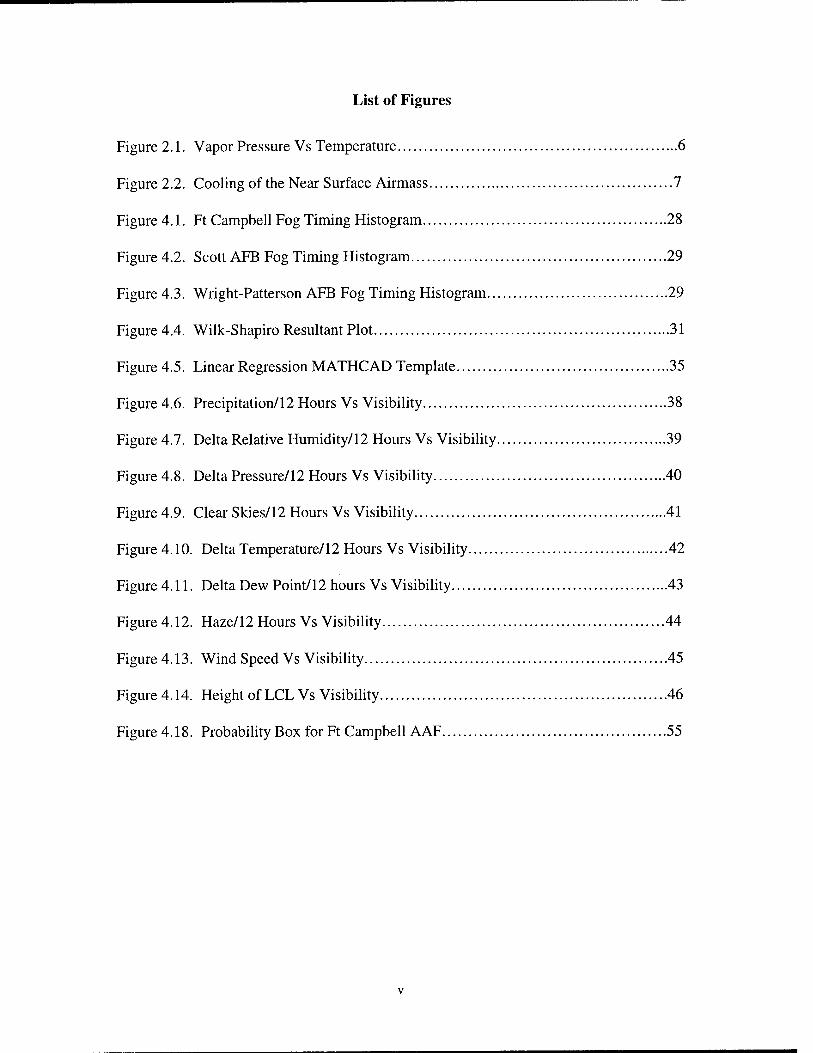
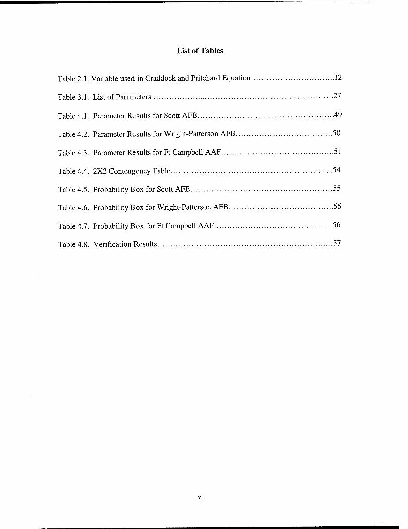


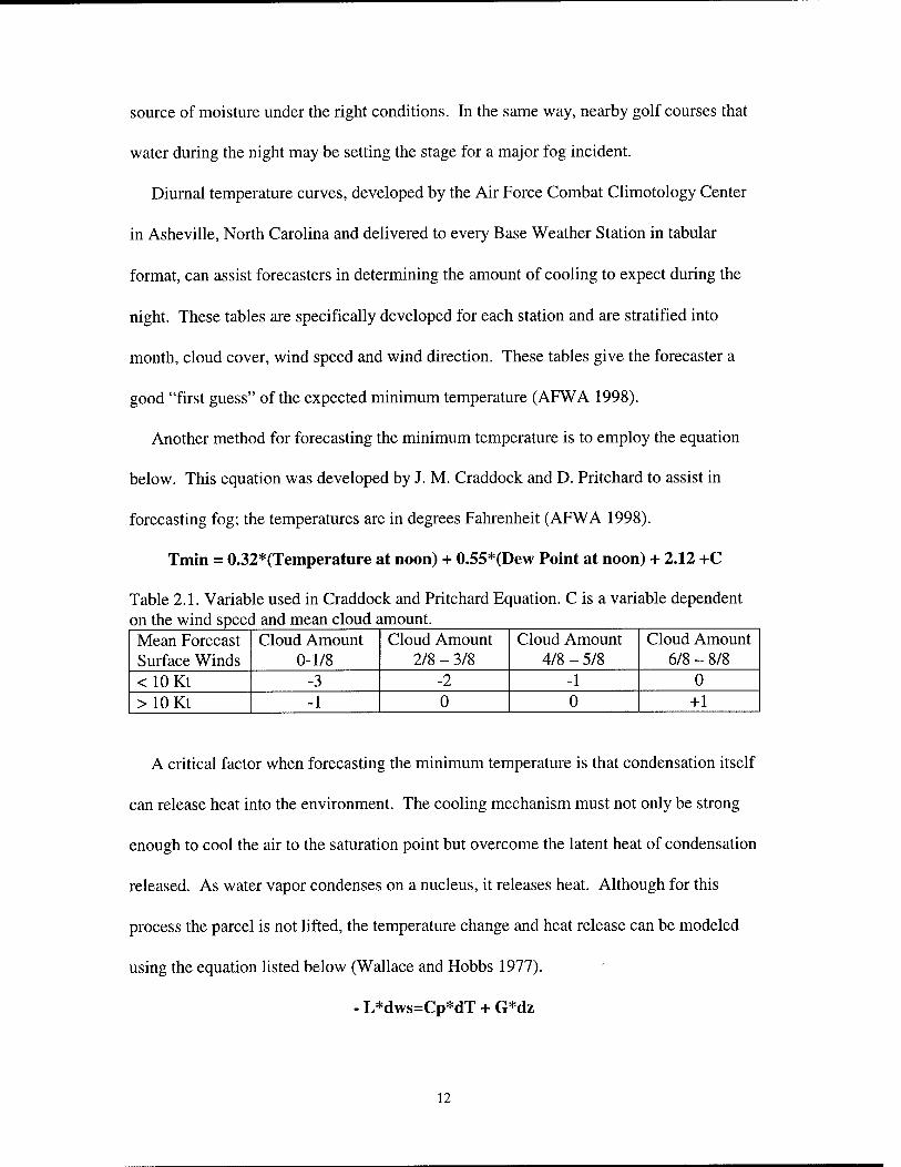

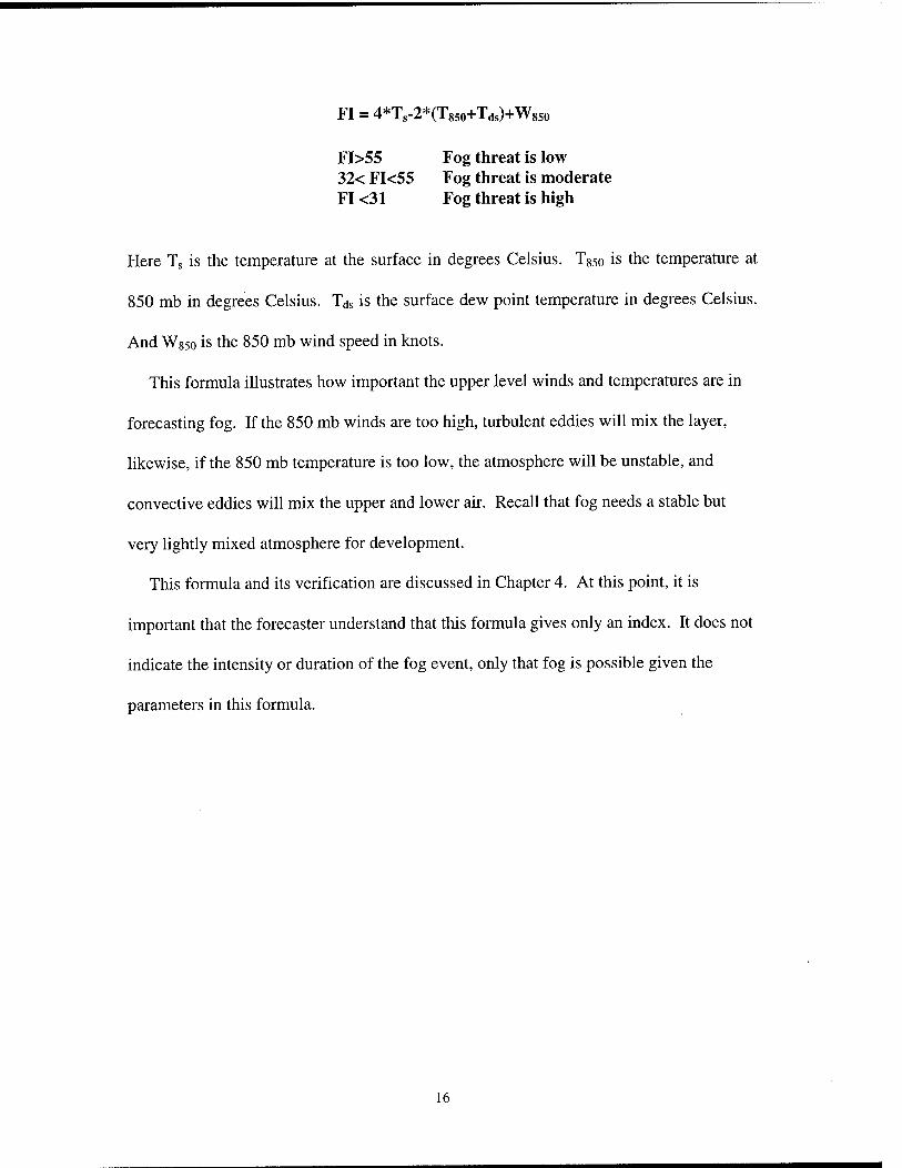


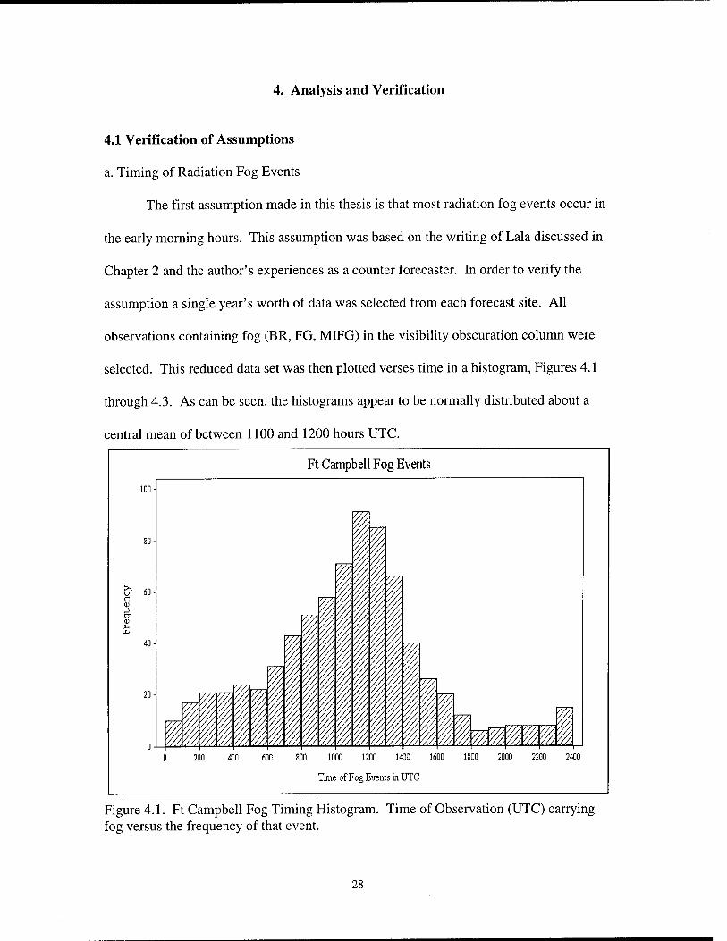

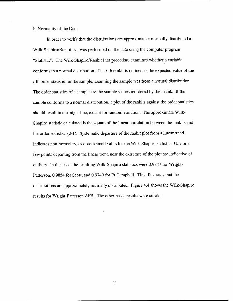
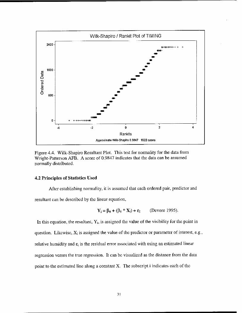


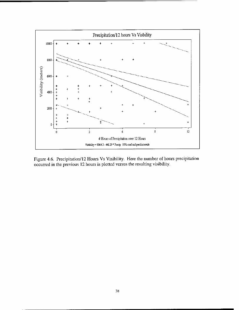

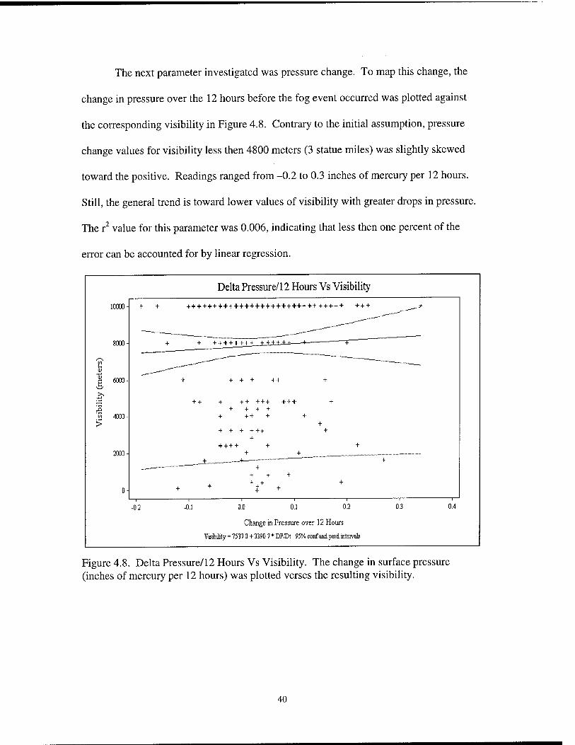
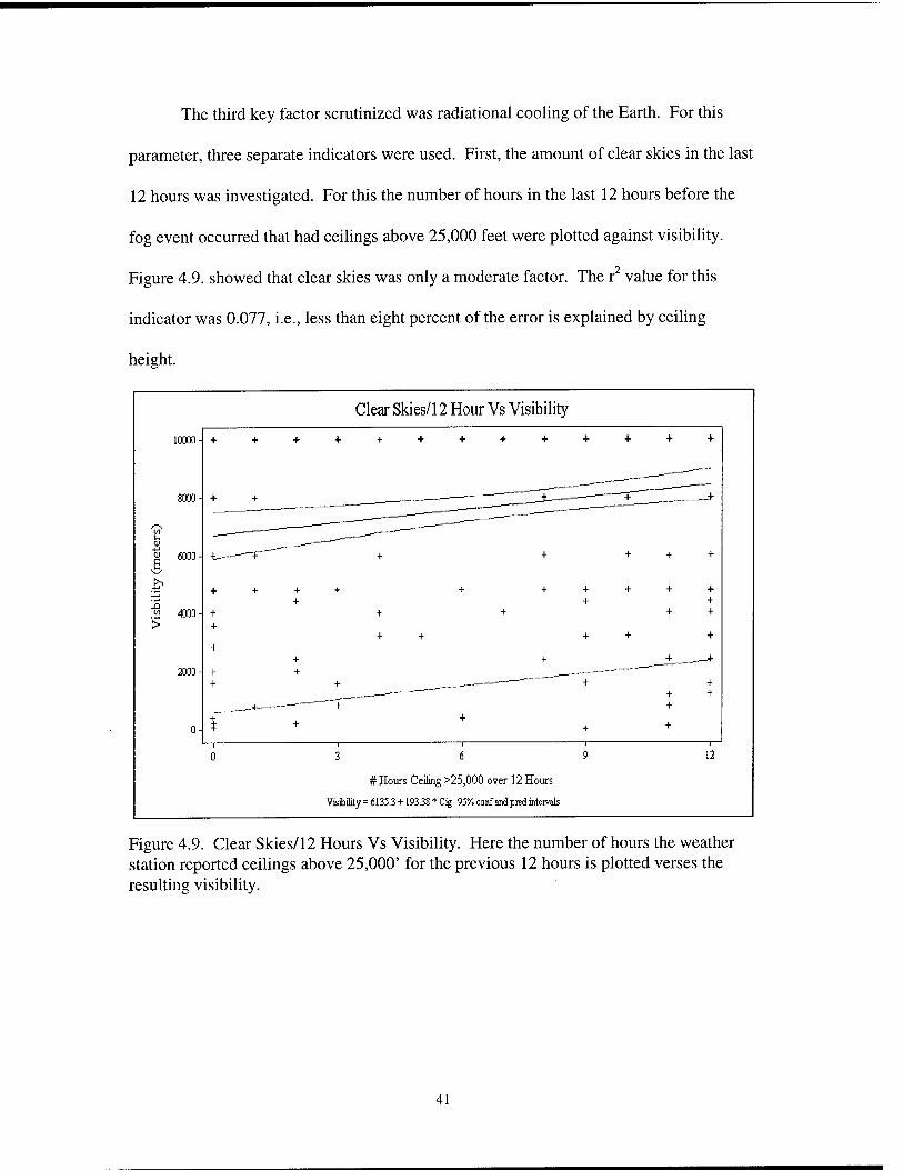


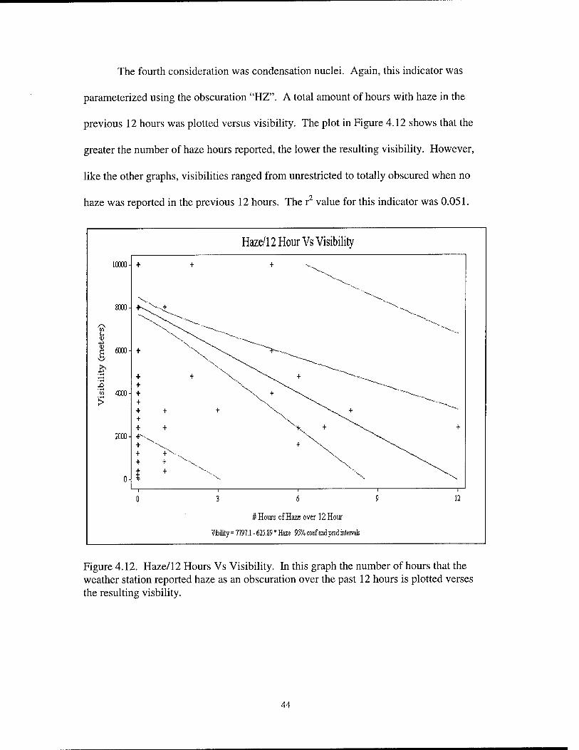


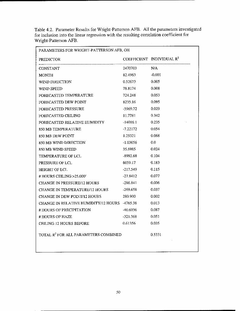


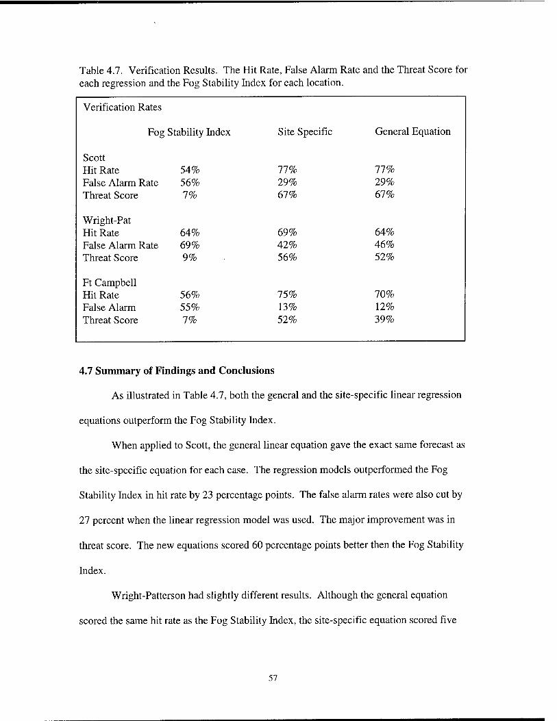


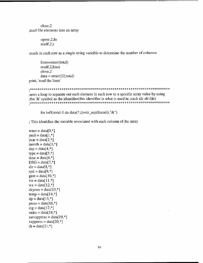


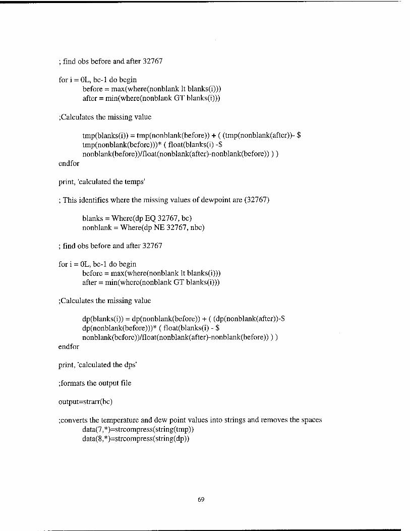

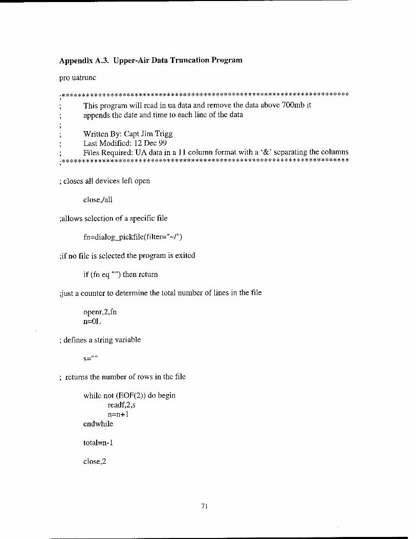
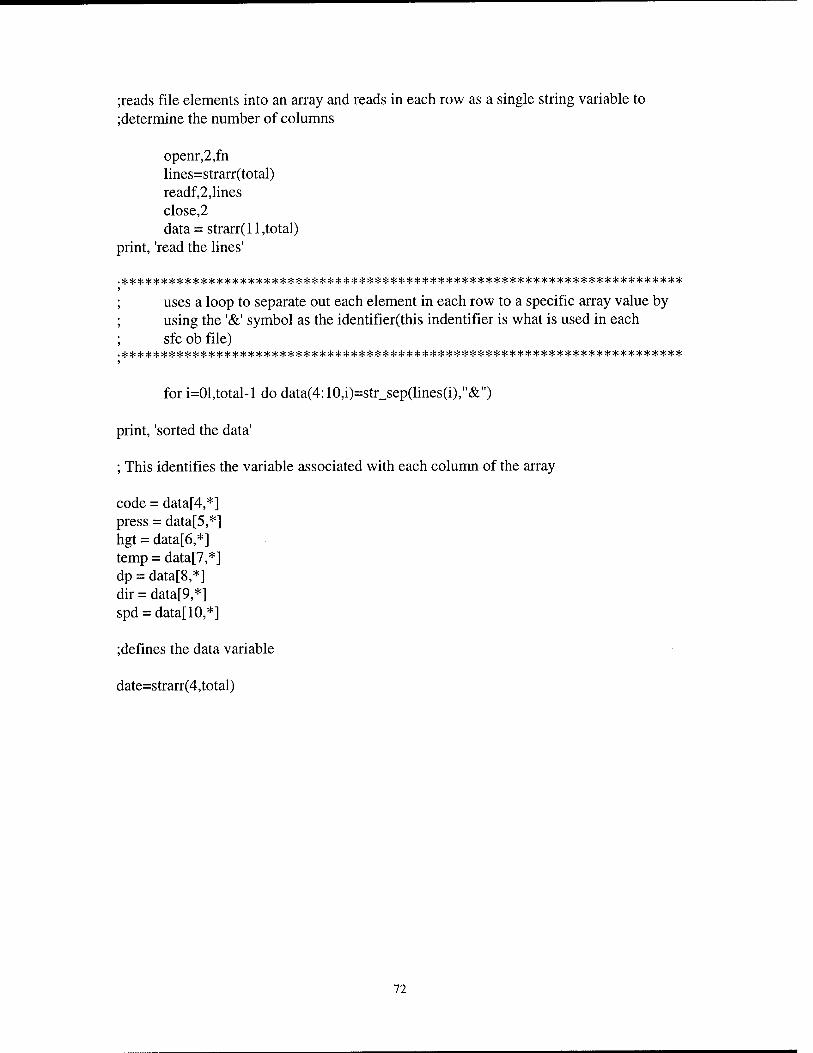


![Vehicular Fog Computing: A Viewpoint of Vehicles as the ...cwc.ucsd.edu/sites/cwc.ucsd.edu/files/Vehicular Fog... · fog computing paradigm [10]–[14]. Specifically, in the fog](https://static.documents.pub/doc/80x56/5ece3cb4a160d21f083aea78/vehicular-fog-computing-a-viewpoint-of-vehicles-as-the-cwcucsdedusitescwcucsdedufilesvehicular.jpg)
