A study of natural usage and sentiment analysis of ...trap.ncirl.ie/2660/1/damiengrouse.pdf · All...

A report submitted in partial fulfillment of the requirements for the

award of the degree of

B.Sc (hons)

in

Computers

By

Damien Grouse (x13114328)

A study of natural usage and sentiment analysis of Electric Ireland and Bord Gais

customers who have moved to smart meters.

1

Declaration Cover Sheet for Project Submission

Name: Damien Grouse

Student ID: X13114328

Supervisor: Michael Bradford

SECTION 2 Confirmation of Authorship

The acceptance of your work is subject to your signature on the following declaration:

I confirm that I have read the College statement on plagiarism (summarised overleaf and printed in full

in the Student Handbook) and that the work I have submitted for assessment is entirely my own work.

Signature: _______________________________________________

Date: ____________

2

Abstract

We've all heard the term, data and most people have an idea of what data is. Data is

information and today it is generally electronically stored. Data can be simply formatted, such

as information on an Excel sheet (integers and characters). Unfortunately, most people struggle

to understand data, unless they see it in a visual representation.

Even the most experienced Data Scientist would struggle to understand a Big Dataset, on initial

inspection. Stored electronic data is stored in a database, in Sql (tabular form) or non-Sql (non-

tabular form) databases. Due to the use of computer languages such as R and software

packages such as R Studio and Microsoft BI. We can query data and return results in a quick and

reliable way. We can also get an easy visualization of the data via graphs, thanks to these

technologies.

Data is acknowledged to only have real value, if the information leads you to an inference or it

is structured and results/insights can be gained from it.

By applying Data Analytics procedures and practices, such as data mining, we can gain a more

incisive understanding of data we are querying, to gain additional knowledge and

understanding.

Keywords: Data; Big Data Set; Data Mining; Data Analytics; R; Software Suites; Graphs

3

Table of Contents Abstract ......................................................................................................................................................... 2

Introduction .................................................................................................................................................. 5

Purpose of this Document ............................................................................................................................ 5

Motivation for this project ............................................................................................................................ 5

Project Sponsor, Partners, Background & Data Sources .............................................................................. 6

Scope of the Development Project ............................................................................................................... 7

Hardware Used ............................................................................................................................................. 7

Methodology KDD ......................................................................................................................................... 7

Project Data .................................................................................................................................................. 8

Data Dictionary ............................................................................................................................................. 8

Project Design and Architecture ................................................................................................................. 11

System ......................................................................................................................................................... 12

Smart meter explained ............................................................................................................................... 13

Technologies Used ...................................................................................................................................... 13

Sentiment Analysis ...................................................................................................................................... 14

Clustering .................................................................................................................................................... 15

Trees ............................................................................................................................................................ 15

Questionnaire Details ................................................................................................................................. 15

Requirements .............................................................................................................................................. 16

Functional Requirements ............................................................................................................................ 16

Non Functional Requirements .................................................................................................................... 16

Environment Requirements ........................................................................................................................ 16

Data Format ................................................................................................................................................ 17

Sentiment Analysis ...................................................................................................................................... 18

Importing the CSV Files ............................................................................................................................... 18

Selecting the Sentiment data ...................................................................................................................... 22

Make up of Survey Demographics .............................................................................................................. 24

Pre-processing the Sentiment data ............................................................................................................ 30

Transforming the Sentiment data ............................................................................................................... 31

Mining the Sentiment data ......................................................................................................................... 32

Evaluating the Sentiment data.................................................................................................................... 32

Sentiment Analysis Conclusion: .................................................................................................................. 36

4

Data Usage .................................................................................................................................................. 37

Selecting the Usage data ............................................................................................................................. 37

Pre-processing the Usage data ................................................................................................................... 37

Transforming the Usage data ..................................................................................................................... 38

Mining the Usage data ................................................................................................................................ 40

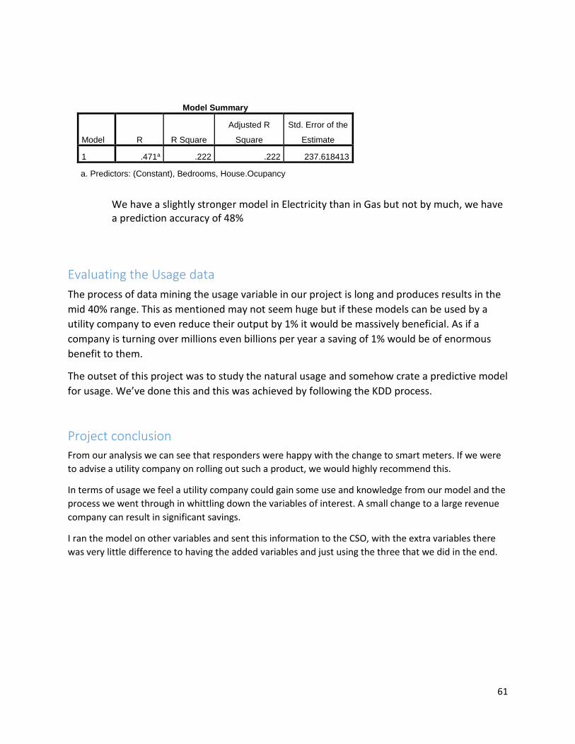
Evaluating the Usage data .......................................................................................................................... 61

Project conclusion ....................................................................................................................................... 61

Overall Project Reflection ........................................................................................................................... 62

Testing ......................................................................................................................................................... 63

Monthly Project Journals ............................................................................................................................ 64

Images ......................................................................................................................................................... 72

5

Introduction

We've all heard the term data and most people have an idea of what data is. Data is

information and today it is generally electronically stored. This electronic data is stored in

databases. Thanks to new technologies and the processing power of these technologies,

coupled with the methodology off data mining, data can now be exploited to gain extra

knowledge. What technology can process, in terms of data processing volume and speed, is

quicker than what a human is capable of. Humans have the knowledge to know what data they

wish to query and gain extra inferences from, such as, are there relationships between data

objects and their strength. Technology cannot make these distinguished decisions yet, it can

statistically see if data interact with eachother, but decision making only occurs unless artificial

intelligence is applied in some measure.

Data Mining is also known as knowledge discovery and data mining (KDD). Data mining is the

extracting of useful structured patterns from data sources (databases, text, images). Patterns

must be valid, novel, potentially useful and understandable.

Data mining is primarily used for predicting outcomes and making more informed decisions,

based on past events, current decision factors, for future events. This is achieved by analyzing

previous occurrences, with machine learning and making predictions on these occurrences. It

allows for the investigation into databases, to find relationships between objects previously

unknown and measure dependencies amongst these objects.

Data Mining methodology is used by humans with technology, to allow humans to make more

informed decisions.

Purpose of this Document

This document describes the processes, procedures and technologies used to complete a final

year software project. It gives a highly detailed account of how the project was completed.

How the data was sourced, extracted and manipulated and the conclusions derived from these

processes.

Motivation for this project

As a final year BSc Computing student in the National College of Ireland, I am tasked to

complete a final year software project. In my final year, I am specializing in Data Analysis. I

chose to apply the new knowledge, theories and technologies introduced to me, during my final

year in college to complete my final year project.

The commercial motivation for this project can be summed up as follows - If we can see

patterns in terms of natural usage, which are re-occurring, it will lead to suppliers of gas and

6

electricity been better able to predict what supply occupants of dwellings need, meaning better

usage predictions for suppliers. With better prediction power and knowledge gained, power

suppliers can use this information to reduce their costs. Better planning, usually means better

returns.

For users of these utility it will be interesting to find if they felt it was worth switching to smart

meters.

Project Sponsor, Partners, Background & Data Sources

ISSDA.

My project supervisor is Michael Bradford, lecturer at national College of Ireland.

Project sponsor John Dunne, CSO.

I contacted the CSO (Central Statistics Office of Ireland) looking for advice and possibly reliable,

clean data and to see if they'd a project they would like me to do on their behalf.

John Dunne(CSO) advised me and gave me information of a project he thought I may find

interesting. It was a trial done by utility companies, Bord Gais and Electric Ireland of moving

their customers from standard meters, to smart meters. He referred me to the ISSDA (Irish

Social Science Data Archive) as they store and control access to the data from the trial. John

told me it would be an interesting topic to study. He said he would be most interested in my

findings regarding domestic natural usage of gas and electricity within the data.

I found the topic and subject matter to be very interesting. I then applied to the ISSDA, to gain

access to the data. I was granted access to the trial data sets from the ISSDA and UCD, once I

signed a terms and conditions document, regarding what I could and could not do with the

data.

The data I was provided, contains data sets of business and domestic dwellings who have

moved from standard meters to Smart Meters installed for their electricity and gas supply and

it also gives me access to pre and post survey results of the participants of the trial.

As per John Dunne’s request, I plan on analyzing and reporting my findings regarding, the usage

data of the domestic users. Thus I am ignoring the data related to businesses.

I also decided seen as the data I was provided with contained pre and post survey

questionnaires, I would also analyze these data sets, as it would be interesting to know if the

utility company’s customers felt the change to smart meters had a positive, neutral or negative

effect on them. This type of analysis is generally known as opinion or sentiment analysis.

7

Scope of the Development Project The goal of this project is to study the data and apply data analytics processes to find natural

usage patterns from the data. I will report my findings to my project sponsor John Dunne from

the CSO. I will also work closely with Michael Bradford, my project supervisor. I will then use

visual displays and software to display my findings. I plan to use the KDD model to get the most

of the data provided to me. This document is also to be taken as a user manual for this project.

The code associated with this project, is to be submitted electronically to my college.

Hardware Used All of the project will be performed on Dell WYSE Pc’s in the college library (spec unknown due

to college It Dept restricting spec details of the machine) and my personal machine, a Toshiba

Satellite Laptop C660, 6 GB of Ram, 750 GB hardrive, Intel Core i3 processor, with a clock speed

of 2.4Ghz. Machine operating system is Windows 10.

Methodology KDD

The term Knowledge Discovery in Databases, or KDD for short, refers to the process of finding

knowledge from data, it is a methodology also. It can be described as a series of steps used to

reach the goal of extracting knowledge from data.

(fig1)

KDD is an iterative process. It involves many stages as the illustration above shows (six in total,

with sub stages between main stages, there are 11 steps).

In a usual Report document, it is assumed there would be use cases. However, as I am using the

KDD model and it is an iterative process, each process will be acknowledged and explained as I

execute the methodology on the data, it is being applied to (there are architecture diagrams

below, fig & fig, this can also be viewed as a use case, of user interaction with this overall

project system).

KDD is an iterative cycle used to mine data and gain knowledge. It is a joyously simple

methodology but very powerful once adhered too and done correctly. KDD is made up of a

number of steps, below is a simple step guide how to apply the KDD process:

8

Step 1: Data, is to get the data.

Step 2: Data Selection, is to understand the data at a high level

Step 3: Target Data, is to select and target data that you wish to use or explore further

Step 4: Pre-processing the data, is cleaning the data into a format it can be analysed, often

most time consuming step of KDD process.

Step 5: Pre-processed Data, at this point the data should be cleaned and ready for exploration

Step 6: Transforming Data, change and manipulate the data to suit your technology and needs

Step 7: Transformed Data, now data is transformed and stored it can now be mined

Step 8: Data Mining, with the previous steps completed correctly, the data can now be mined,

using machine learning and analysis algorithms.

Step 9: Patterns can be visible (if there are any), use clustering, trees and statistical analysis to

show these patterns

Step 10: Evaluate and Interpret the results

Step 11: Once the process of KDD has been complete, additional knowledge from the data and

intricate object relationships should be known as well as effect objects have or have not had on

each other.

As KDD is an iterative process, to reach the goal of additional previous unknown knowledge, the

process may have to be applied more than once.

Project Data

Data used in this project, as previously mentioned came from ISSDA. The format this data

received in was a combination of Microsoft Word, for the questionnaires. Text and CSV files

contained the data relating to the usage.

Data Dictionary

Manifest: Smart Meter Electricity Trial data

Issued by: The Research Perspective Ltd

Date: 12-03-2012

(1) Smart meter read data: 6 zipped files named File1.txt.zip to File6.txt.zip each containing 1 text file

Format of each data file: 3 columns corresponding to

9

Meter ID

Five digit code:

Day code: digits 1-3 (day 1 = 1st January 2009)

Time code: digits 4-5 (1-48 for each 30 minutes with 1= 00:00:00 –

00:29:59)

Electricity consumed during 30 minute interval (in kWh)

(2) Pre and post trial residential surveys: 2 word files: “RESIDENTIAL PRE TRIAL SURVEY”, “RESIDENTIAL POST TRIAL SURVEY” containing

CATI coded surveys

2 excel files: “Smart meters Residential pre-trial survey data”, “Smart meters Residential post-

trial survey data”

Format of file:

First row: question number and summary

Subsequent rows: 1 row per respondent

ID = meter ID

1 column per survey question

(3) Pre and post trial SME surveys: 2 word files: “SME PRE TRIAL SURVEY”, “SME POST TRIAL SURVEY” containing CATI coded

surveys

2 excel files: “Smart meters SME pre-trial survey data.xls”, “Smart meters SME post-trial survey

data.xls”

Format of file:

First row: question number and summary


ID = meter ID


(4) Allocation file: 1 excel file “SME and Residential allocations”

Format of file:

ID = meter ID

Code= specify residential, SME or other categories

10

Residential stimulus = for residential participants, the stimulus code (see

published report for details)

Residential tariff = for residential participants, the tariff category (see published

report for details)

SME allocation = for SME participants, the stimulus (see published report for details)

Manifest: Smart Meter Gas Trial data

Issued by: The Research Perspective Ltd

Date: 15-10-2012

(5) Smart meter read data: 78 Microsoft excel files named GasDataWeek0 to GasDataWeek77

Format of each data file:

ID = meter ID

DT = five digit code:

Day code: digits 1-3 (day 1 = 1st January 2009)

Time code: digits 4-5 (1-48 for each 30 minutes with 1= 00:00:00 –

00:29:59)

Used = Gas consumed during 30 minute interval (in kW)

(6) Pre and post trial residential surveys: 2 word files: “RESIDENTIAL PRE TRIAL SURVEY - GAS”, “RESIDENTIAL POST TRIAL SURVEY - GAS”

containing CATI coded surveys

2 excel files: “Smart meters Residential pre-trial survey data - Gas”, “Smart meters Residential

post-trial survey data - Gas”

Format of file:

First row: question number/description


ID = meter ID


(7) Allocation file: 1 excel file “Residential allocations”

Format of file:

ID = meter ID Allocation = for participants, the stimulus code (see

published report for details)

11

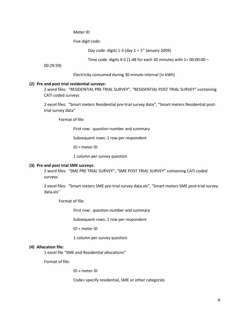
Project Design and Architecture

Architecture used in this project, will be to import data files into R Studio, then the KDD process

will be applied and will be, until the iterative process has been exhausted and all required

inferences from the data will have been gained.

High Level Architecture (also can be viewed as use case of user interacting with the Project System)

Begin KDD Process Import Data to KDD

Re-iterate

(fig2)

Data

Target Data

Pre-processed

Data

Transformed

Data

Data Mining

Interpretation/

Evaluation

Knowledge

12

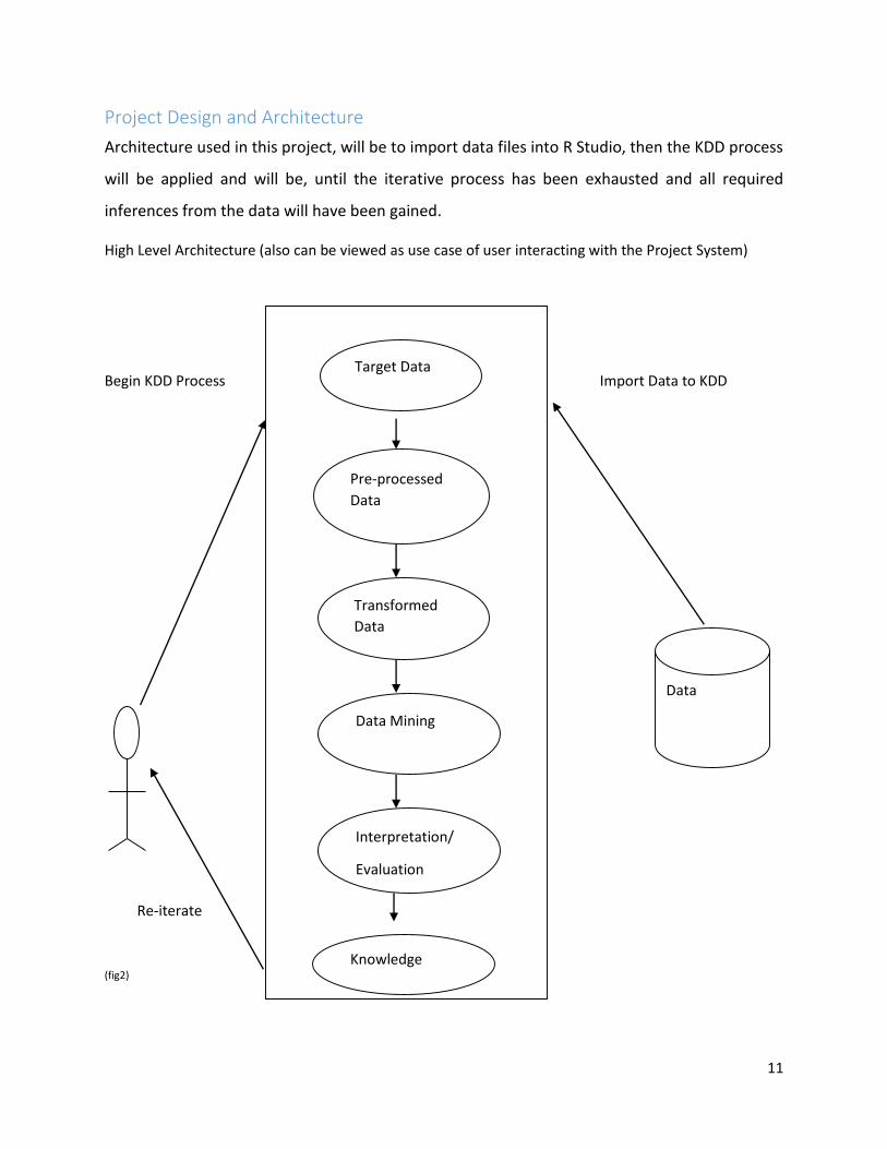
System

The project is not a typical software engineering project. However, it is planned to use many procedures and processes of building a software project into the project and system. By this we mean for example, we will adhere to separation of concern to build the project and system, systematically. Parts will be kept separate but will interact when called upon. For example, the data will be stored separate from the system, it will only come into play when it is called into the staging area. The system will not adhere to traditional software application design, as we are performing a data analysis on data sets.

However, to keep our explanation similar to a typical system, we will be interacting with csv files, importing them into R Studio, Weka, Sql Workbench, IBM Spss and Microsoft BI and performing data manipulation, querying the data and then displaying our results and findings, in numerical and visual displays.

(fig 3)

(tableau was replaced by Microsoft for the presentation of this project. R, Weka and IBM Spss were used

as staging areas and visuals in this document are from these technologies).

13

Smart meter explained

A smart meter is an electronic device used to measure the consumption of energy. In this case

it is been used to record to usage of electricity and gas on both domestic and business usage. It

records and sends data to the service provider at pre-programmed intervals throughout the day

and night (in our data this occurs every 30 minutes). It allows two-way communication between

the meter and the service providers central system. To do this the meter needs to be able to

connect to the internet.

The smart meter can also be used by customers who have an application on an electronic

device such as a smart phone, which can connect to the internet. Users of the app, can use it

similar to their thermostat timer in their house. They can program when the heating or hot

water is to come on and off and monitor their usage. Hive is an example of this service (Bord

Gais).

Technologies Used

The technologies used during the project were:

R studio

R (computer programming language)

Windows Office suite

Microsoft Power BI

PowerShell

IBM Spss Statistics

Weka

R studio is an IDE (integrated development environment), for writing R code. Similar to how

NetBeans is an IDE for writing Java code. R is open source, meaning to download and use it is

free. R is a computer language primarily used for statistical analysis and production of graphics

of data. R Studio is the environment which this occurs. It was developed by Bell Laboratories

(now Lucent).

R Studio uses packages published by users and its creators to add functionality to the IDE. Such

as the package “ggplot2”, which allows users to make more creative graphs from their data. To

use a package, you need to install it and to use it, you call it into your environment using the

library command. R was chosen as the primary language of my project, as it is a language

specifically for dealing with statistics and visual displays of data. We were introduced to R in our

4th year of college and it has been found to be a very rewarding language to work in. R studio is

the IDE for R, so it was used in this project as R and R Studio go hand in hand.

14

Windows office suite lent itself to the project as Excel was used to open and view the CSV files

associated with this project. Microsoft PowerPoint was used to generating mid-point and final

presentation slides. Microsoft Word was used to write up reports and to view questionnaires.

Microsoft Power BI Desktop (Business Intelligence) is a free desktop application which allows

the user to import their datasets for data exploration and visualisation through the creation of

graphs.

PowerShell is a command-line based service on Windows operating machines. It is generally

used for scripting language and command-line shell. It is powerful as it is the closest layer of

interface a user has to the actual nuts and bolts of a computer and what is stored on that

computer. It excels in processing text and numeric data quickly.

IBM Spss Statistics is a Statistical Package for the Social Sciences. It is a software suit which can

read data sets stored in a CSV file and perform highly complex data analysis and manipulation.

Weka is a free software suite containing machine learning algorithms for data mining tasks, it

can be directly applied like IBM Spss to a data-sets but Weka contains tools for data pre-

processing, classification, regression, clustering, association rules and visuals. Weka was chosen

as these features lend themselves well to the KDD process.

Sentiment Analysis

The data supplied by the ISSDA came in pre and post survey CSV and Word files containing

respondents answers to the survey questions. There are two files each for both Bord Gais and

Electric Ireland customers, pre-trial and post-trial surveys, totalling four files to be used in our

analysis.

Sentiment analysis (also known as opinion analysis), is generally accepted as the measuring of

how “something” made a person feel or the effect it had on them. This something can literally

be anything, once it can be quantified/measured. The measurement generally used is, did

“something” have a positive, neutral or negative effect on a person/groups. The degrees of

measurement are, positive, neutral and negative and these can also be subdivided into

measurements.

A simple example is observing humans looking at pictures. If they are looking at distressing

pictures (a person crying), the person would generally feel negative. If they see happy pictures

(a person smiling), they generally feel positive.

The person could then be asked to what degree of a positive effect did a happy picture have on

them, for example, yes the picture made me happy, responder could then be asked to rate their

level of happiness from a score of 1 to 5, 1 been happy and 5 been deliriously happy.

15

In the case of this project, we are testing if the move from normal meters to smart meters had

a negative, neutral or positive effect on those surveyed. Sentiment analysis is usually associated

with text but in this project we are going to use the process of sentiment analysis on text as

well as numerical data.

Gas & Electric Smart Meter Sentiment Hypothesis, would be that the,

Null Hypothesis: change to smart meters had no effect on users.

Alternative Hypothesis: there was an effect on users who changed (positive/negative)

Clustering

Clustering is a data mining technique for getting a good initial overview of the data and looking

for natural groupings amongst the data. It is called an unsupervised learning, as we have no

idea what we are going to find but more specifically we have no pre-determined outcome in

mind, we are hoping to learn or see clusters within the data.

Unlike supervised learning, which is the process of extracting knowledge from data with a

specific purpose or goal in mind.

Trees

Trees are a data mining tool used for classification. It is like Clustering and unsupervised

learning. A data tree is usually referred to as a decision tree. In essence a decision tree is simply

a flow chart, were users can follow the data until it reaches the end of a path, returning an

answer or classification. Classification is when something has a label on it. For example, a

decision tree has a root, which is the whole dataset usually, the branches are decisions and the

leaves are end points, also known as decision nodes. If we parse a piece of data through a data

tree, when it gets to a decision node, the data then takes on the label of that node. This is

classification, when data is labelled.

Questionnaire Details

The survey was done in two parts. Firstly, respondents were asked a series of questions

regarding themselves individually (their sex), their home (do they live alone, how many people

they live with, how many bedrooms are in their home), there social status (income, are they

self-employed, an employee.), the main reason they took part in the trial (monetary, help the

environment) and what they expected to get from the trial (save on their utility bills and a

cleaner environment) and other questions.

They were then asked the same set of questions, towards the end of the trial.

16

These surveys were done for both Bord Gais and Electric Ireland customers, the questions on

both surveys we almost exactly the same apart from slight alterations.

I will use both sets of questionnaires, pre-trial and post-trial, to compare and to see if the move

to smart meters had any (negative/positive) or no (neutral) effect on responders.

I will follow the KDD methodology to fulfil the sentiment analysis

Requirements

User is to, must be able to read, understand and follow this document, regardless of their

technical knowledge. All inferences are to be made without prejudice or pre-conceived desired

inference.

Functional Requirements

I. All data used,, manipulated, relabelled and transformed must derive from the original data sets

issued by the ISSDA

II. Software been used must be able to read and import data files

III. Software must be able to manipulate the data to the user’s requirements

IV. Software must be able to return visual display of data

V. Software must be able to process large amounts of data and return inference.

VI. User must be competent in using software

VII. Understand the data

VIII. Analyse natural usage and sentiment data

IX. Report my findings

Non Functional Requirements

I. All code must be commented so it is easily understood.

II. A reader of this final report should not require a high technical level of understanding to be able

to understand the findings.

Environment Requirements

I. Use computers compatible with the chosen software of this project

II. Use computers with resources to perform all computational tasks.

17

Data Format

The Word documents contain the questions used by both domestic Gas and Electric pre-trial

and post-trial responders. These files we used as a reference to gain meaning for the values

inserted into the respondent’s answers, contained in the CSV survey files.

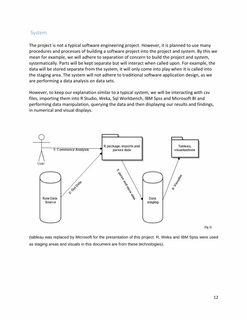
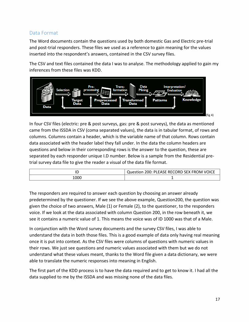
The CSV and text files contained the data I was to analyse. The methodology applied to gain my

inferences from these files was KDD.

(fig 4)

In four CSV files (electric: pre & post surveys, gas: pre & post surveys), the data as mentioned

came from the ISSDA in CSV (coma separated values), the data is in tabular format, of rows and

columns. Columns contain a header, which is the variable name of that column. Rows contain

data associated with the header label they fall under. In the data the column headers are

questions and below in their corresponding rows is the answer to the question, these are

separated by each responder unique I.D number. Below is a sample from the Residential pre-

trial survey data file to give the reader a visual of the data file format.

ID Question 200: PLEASE RECORD SEX FROM VOICE

1000 1

The responders are required to answer each question by choosing an answer already

predetermined by the questioner. If we see the above example, Question200, the question was

given the choice of two answers, Male (1) or Female (2), to the questioner, to the responders

voice. If we look at the data associated with column Question 200, in the row beneath it, we

see it contains a numeric value of 1. This means the voice was of ID 1000 was that of a Male.

In conjunction with the Word survey documents and the survey CSV files, I was able to

understand the data in both those files. This is a good example of data only having real meaning

once it is put into context. As the CSV files were columns of questions with numeric values in

their rows. We just see questions and numeric values associated with them but we do not

understand what these values meant, thanks to the Word file given a data dictionary, we were

able to translate the numeric responses into meaning in English.

The first part of the KDD process is to have the data required and to get to know it. I had all the

data supplied to me by the ISSDA and was missing none of the data files.

18

Firstly, for both gas and electric responder’s, we viewed the Word documents, to understand

the survey format, the questions been asked and how the answers were determined and their

meaning. By doing this I had a familiarity and a clear understanding of the survey. Below is an

example of how the Word documents are formatted:

QUESTION 300

May I ask what age you were on your last birthday?

INT: IF NECCESSARY, PROMPT WITH AGE BANDS

1 18 - 25

2 26 - 35

3 36 - 45

4 46 - 55

5 56 - 65

6 65+

7 Refused

We can see the question above and the possible answers the respondent has to choose from. In

the CSV file associated with this question, we would then look at the response from the

responder and from there gain our knowledge of what their response meant.

Once we were familiar with the questionnaire and the CSV files, the KDD process was begun for

the sentiment analysis. The files holding the survey data used for both Gas and Electric

customers, came was in CSV format.

Sentiment Analysis

Importing the CSV Files

The environment which was chosen to analyse the gas and electric responders for sentiment

analysis, was R Studio. As we had the data needed in CSV files already, it was just a process of

importing the files into R. It was also necessary to have the correct packages installed to R

Studio for functionality purposes and to call the libraries associated with those packages into

our staging area, so we could use these packages.

Below is the code for installing these packages and for setting the working directory and

importing the required CSV file to begin data exploration (below you can see how the packages

are installed, libraries initiated, the working directory is set and data from csv files is imported

into R and relabelled, in the below case it is called “PreSent” these steps were followed every

time for importing CSV files during this project, for this reason I will only explain this step once,

for sake of repeating myself.)

19

#install packages and Libraries needed

install.packages(c("e1071", "C50", "ggplot2", "dplyr",

"foreign", "hexbin","descr", "caret", "e1071"))

#call in libraries to this script

library(e1071)

library(hexbin)

library(ggplot2)

library(caret)

library(descr)

library(C50)

library(zoo)

library(dplyr)

library(foreign)

#set working directory

setwd("H:\\SoftwareProject\\CER_both\\CER Gas Revised October

2012\\GasSentimentAnalysis")

#confirm in correct directory

getwd()

#list what is in the current directory

dir()

#import file I wish to use now and label it PreSent

PreSent = read.csv("Smart meters Residential pre-trial survey

data - Gas.csv", sep = ",", header = TRUE).

Once the above code is run, we now have the packages installed, they have been called into our

environment, the working directory has been set (is the path the machine needs to know from

where the file is that we want to import into R Studio) and the file we wish to work on has been

installed and relabelled. From here I can query the data, manipulate it, join the data and display

my findings using graphs.

20

Initially in R Studio, in the environment pane, we can see this file has 1365 objects and 156

variables. This means we have 1365 rows of data and 156 column headers or we can also say

we have 1365 Gas customer’s and 156 questions that each customer was asked to answer.

When the Electric file was imported we have 4232 objects and 144 variables or 4232 Electric

customers and 144 questions.

In the Gas case we have the file of the pre-trial survey data of gas responders. When importing

the CSV file, the data was given a label (name) called “Present”. R now sees all the data

associated with the CSV file but now in a data frame called Present.

So we now have our data in R Studio, we now need to explore and get to know it, which is step

1 of the KDD process complete.

(From here is a step by step guide of the whole KDD process, performed on the Gas customer’s, for the sentiment

analysis phase of this project. The same process was performed for the Electric customers, to avoid repeating

myself, I will only write up the process of the gas customer’s, till I get to the evaluation of both set of customer’s

unless otherwise stated.)

Now we want to gain knowledge and explore the dataset. To do this, we can run the following

commands to view all the data to get a general feel of the data,

#see the data…. lists the data in R

PreSent

#this will list the headers of each column/questions at top of

each column

names(PreSent)

#this command shows us the data in R Studio in format it is in,

in the CSV files

View(PreSent)

#this command shows us the structure of the data, the type of

data stored in an attribute, i.e. Question101 = int.

str(PreSent)

#this command shows us the number of attributes associated with

the data.(in this case 1365)

attributes(PreSent)

#this summary command gives us the summary of all the data

associated with the PreSent data set, it lists all questions and

their Min,1st quantile, Media, Mean, 3rd Quantile and Max values.

summary(PreSent) # below is example of summary output

21

Question.474..Have.any.of.the.following.ever.applied.to.you...None.of.these

Min. :0.0000

1st Qu.:0.0000

Median :0.0000

Mean :0.1143

3rd Qu.:0.0000

Max. :1.0000

NA's :1330

After getting to know the data for the sentiment analysis, which was very time consuming, due

to exploring the amount of variables associated with the data (156), the awkwardness of how

the variables(questions) are written and displayed in the CSV files. Questions are very long and

could not be fully seen in the CSV files unless, expanding the column width. Indeed, the files

were initially imported into Sql. CSV file was inserted into Sql Workbench but the variable

names caused endless trouble and this ws abandoned, as it was deemed too time consuming to

change almost 300 variable names. A connection was set up to the Sql database via R Studio

but it was not used due to variable naming issue (code below shows Sql connection via R).

#map to working directory I've project folder in

#code to read the csv file

dataPre <- read.csv("Smart meters Residential pre-trial survey

data - Gas.csv",header=TRUE,stringsAsFactors= TRUE,sep=",")

#comand will currently list survey questions and display

answeres as integers

con <- dbConnect(RMySQL::MySQL(),

dbname = "damien1",

host = "STLABS-17-092",

port = 3306,

user="DamienProj",

password="milan1978")

dbListTables(con)

dbReadTable(con,"smart meters residential post-trial survey data

- gas")

In R the variable names are easier to see but they are still awkward to view, as the opposite

view in the csv file, where the questions are headers and read from left to right. In R the can be

viewed this way or in a list format but due to the sheer volume of questions, it is terribly

22

difficult to view all the data and gain an easy understanding of it. To gain a good level

understanding of the data, it took a few weeks to get to grips with it mentally. As we were still

studying attending class and producing assignments. Plus, there were two sets of customer’s

we were working to understand.

See the example below, it shows how we targeted each variable(Questions) to understand it’s

output, by placing the question and it’s data into a data table, we then see the results but the

result has no meaning, so we have to add labels, to give the data meaning:

#Make Q200 into a data table

> table(PreSent$Question.200..PLEASE.RECORD.SEX.FROM.VOICE, useNA='ifany')

1 2

711 654

> #returns values 1 and 2, 1 = male, 2 = female respondents

> #Ans to Q200 is either male(1) or female(2), lets class these options

> PreSent$Question.200..PLEASE.RECORD.SEX.FROM.VOICE<- factor(PreSent$Questio

n.200..PLEASE.RECORD.SEX.FROM.VOICE,

+ levels=c(1, 2),

+ labels=c("Male", "Female"))

> # this will show us the male to female slpit

> summary(PreSent$Question.200..PLEASE.RECORD.SEX.FROM.VOICE)

Male Female

711 654

> # so the respondents are 711 males & 654 females

This process was repeated on each question that was used in this project.

Selecting the Sentiment data

Once an understanding of the data had been reached, it was on to step two of the KDD process,

data selection. Two scripts were created in R for both gas and electric customers to analyse the

sentiment analysis, these scripts are similar to all the code associated with this project (for the

sake of again not repeating myself, we will concentrate on the gas sentiment analysis in this

document, though the evaluation will include both sets of gas and electric customers.)

We needed variables with outputs which could be used to give us an inference into whether

customers felt (an effect) moving to smart meters was or was not beneficial to them or of

neutral benefit. To do this variable where needed, to give an insight into why users had taken

part in the trial. As our overall knowledge of the data was good at this point, we applied this

knowledge to identify variables that would return an inference.

Two options sprang to mind, time and money as two variables to be used to measure

sentiment. As time was not a factor in this trial (other than the duration the trial ran for), it was

decided to concentrate on monetary values as a reason a responder would join the trial. This

logic lead to the following questions been identified as sources for establishing responder’s

23

sentiment to the change to smart meters. The following questions and answers we’re identified

as our sources for sentiment analysis.

QUESTION 5011

I am interested in reducing my gas bill and I hope that I will as part of the trial

1 1-is very close to your reason

2 2

3 3

4 4

5 5 is not at all a reason.

QUESTION 5414

How do you think that your gas bills will change as part of the trial?

1 No change

2 Increase

3 Decrease

QUESTION 54155 IF [ Q5414 , 3 ]

By what amount?

1 less than 5%

2 between 5% and 10%



5 more than 30%

6 don’t know

Asking if reducing their bills was the motivation for users to sign up to the trial. It is a simple

way of evaluating their reason for been on the trial. Also the same questions appear in the post

survey. So by been able to compare whether users saved money or not, is a logical

measurement to gaining how they felt the trial was for them. As everyone likes to save money

and a reduction on the amount been spent by a customer is deemed a positive outcome.

24

Make up of Survey Demographics

While getting to know the data, we thought it would be beneficial to get an idea of the

demographics of who was been surveyed. The following analysis was performed on the pre-

survey data for both gas and electric customers. This was done for both gas and electric

customers. R Studio was used for this exploration. The survey files were imported into R Studio

and a script was created for gas and electric.

Gas Survey Demographic

Firstly, we want to know the male and female makeup of the gas responders, this was done by

tabling Question.200 and labelling the outcome, which returned the following output,

summary(PreSent$Question.200) Male Female 711 654 The same was done for the electric responders, which returned the following data,

summary(PreSentElect$Question.200..PLEASE.RECORD.SEX.FROM.VOICE) Male Female 2127 2105

Now we know the sex breakdown of the groups, we can check the age groups of the

responders, for the Gas users this data was associated with Question.300, the result output is

below with a graph exported from R studio and a table showing how many responders fell into

each group,

summary(PreSent$Question.300) 18-25 26-36 36-45 46-55 56-65 65+ Refused 5 195 371 330 222 231 11

25

The electric responders age groups can be seen below,

summary(PreSentElect$Question.300) 18-25 26-36 36-45 46-55 56-65 65+ Refused 16 420 905 1031 883 953 24

26

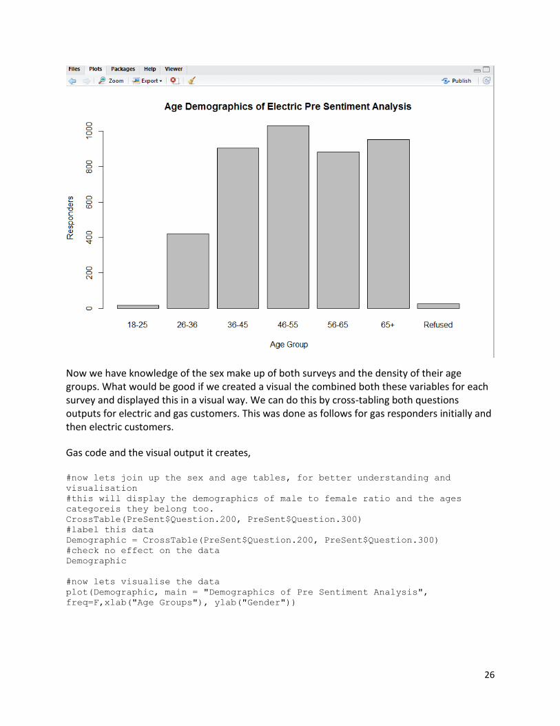
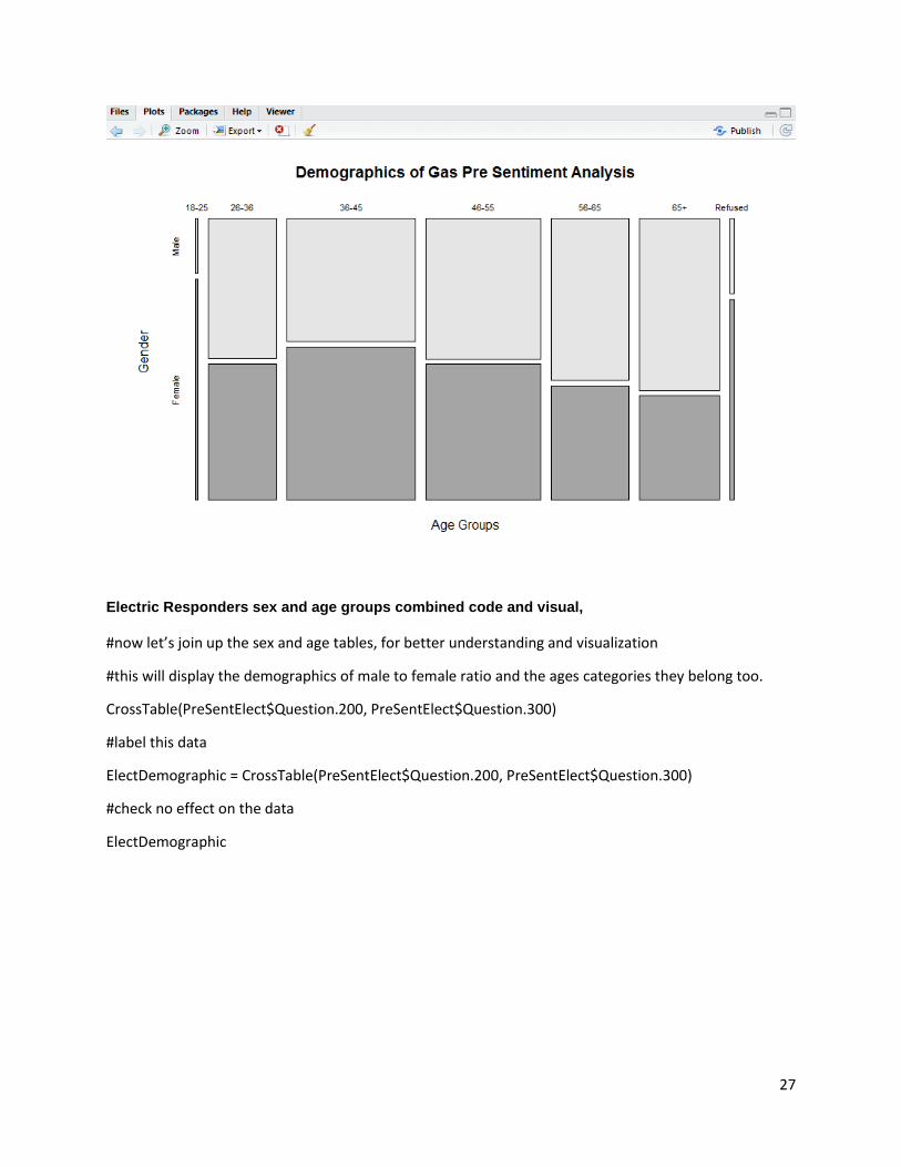
Now we have knowledge of the sex make up of both surveys and the density of their age groups. What would be good if we created a visual the combined both these variables for each survey and displayed this in a visual way. We can do this by cross-tabling both questions outputs for electric and gas customers. This was done as follows for gas responders initially and then electric customers.

Gas code and the visual output it creates, #now lets join up the sex and age tables, for better understanding and

visualisation

#this will display the demographics of male to female ratio and the ages

categoreis they belong too.

CrossTable(PreSent$Question.200, PreSent$Question.300)

#label this data

Demographic = CrossTable(PreSent$Question.200, PreSent$Question.300)

#check no effect on the data

Demographic

#now lets visualise the data

plot(Demographic, main = "Demographics of Pre Sentiment Analysis",

freq=F,xlab("Age Groups"), ylab("Gender"))

27

Electric Responders sex and age groups combined code and visual,

#now let’s join up the sex and age tables, for better understanding and visualization

#this will display the demographics of male to female ratio and the ages categories they belong too.

CrossTable(PreSentElect$Question.200, PreSentElect$Question.300)

#label this data

ElectDemographic = CrossTable(PreSentElect$Question.200, PreSentElect$Question.300)

#check no effect on the data

ElectDemographic

28

From looking at both graphs and their make ups, we see striking similarities amongst gas and

electric responders. The majority of those surveyed are made up by the 36 to 56 years of age.

The amount of women been surveyed decrease in as age increases. There are very few been

surveyed are in the 18 to 25 age group.

We also wanted to vusialize the following Question for both gas and electric users, as part of

researching the respondents living arrangements,

Gas Living Arrangements (code and vusual),

table(PreSent$Question.410..What.best.describes.the.people.you.live.with.)

summary(PreSent$Question.410..What.best.describes.the.people.you.live.with.)

#shorten variable name

PreSent$Question.410 =

PreSent$Question.410..What.best.describes.the.people.you.live.with.

#check data is the same

summary(PreSent$Question.410)

#it is now move on and factor and label the data

PreSent$Question.410= factor(PreSent$Question.410, levels = c(1,2,3), labels

= c("Live alone","All people over 15 years of age",

29

"Both adults and children under 15 years of age "))

#this gives us clearer understanding of the trialists

summary(PreSent$Question.410)

#change variable name

LivingDemographic = PreSent$Question.410

#no effect on the data

summary(LivingDemographic)

#lets visualise the variable

plot(LivingDemographic, main =" Gas Pre-Survey of who you live with")

We can see from the gas graph above that most people are living with children over 15, the

second largest group is made up of adults and young children and the smallest group are those

that live alone.

The same code was applied to the Electric responders, below is the graph,

30

Similar to the gas, the same results can be applied to the electric responders. This lead us to the

conclusion that the area been surveyed is a mature area, due to the amount of people living

alone and who are adults with children over 15.

Pre-processing the Sentiment data

Once the data was identified that we wanted to work on, the variables(questions) were made

into individual data tables. These tables are simple tabular structures, with the question as the

header and all the data associated with that question in rows beneath it. Another reason for

doing this, was similar to software development theory of separation of concerns. In other

words, each piece of software you are working on, should be separate to itself and not see or

be seen by any other object (unless allowed), so interference cannot occur between objects,

leading to an effect on the results.

Once the tables were created, we did not want any rows to be empty, we wanted to get as

clear a picture of the outputs to the variable as possible. To prevent data loss and not to create

any outputs that may skew the data, “NA’S” were used for missing outputs for each table. This

is a common process to follow in data analysis. Others processes may ad “0" or the average of a

data set rows to replace empty values, but as our data was numeric, these options were felt

may have had an effect on the output for the variable. So we used NA’s for missing values.

31

Transforming the Sentiment data

As the answers are options the responder has to choose from (predetermined responses), there

had to be some changes applied to the output, to allow for clearer understanding of the output.

For example, instead of the following:

QUESTION 5011

I am interested in reducing my gas bill and I hope that I will as part of the trial

1 1-is very close to your reason

2 2

3 3

4 4

5 5 is not at all a reason.

The following changes were made to the responses to Question 5011:

"Main Reason",

"Strong reason",

"Good reason",

" Medium Reason",

"Not strong at all"

We replaced the 1 to 5 answers from the survey. These outcomes have the same meaning but

put the scoring range into a more understandable context. Also as the question is very long, it

does not lend itself to being clear to work with in CSV or in R-Studio. As mentioned previously,

separation of concerns theory was applied to examining the data, we want to isolate the

variable under a new label. In this case, as with other questions used as objects in this project,

the question was renamed and a label was applied, this was achieved as follows,

PreSent$Question.5011Savings =

PreSent$Question.5011..I.am.interested.in.reducing.my.gas.bill.a

nd.I.hope.that.I.will.as.part.of.the.trial.

In essence the "Present" label is the whole data set for the survey, by adding a “$” after this,

means we are examining a subset of the whole data frame, in this case “Question.5011…”.

By PreSent$Question.5011Saving = followed by the question, we are creating an instance of

that question but in a variable named “PreSent$Question.5011Savings”, which is much clearer

and easier to work with.

These data transformations are applied constantly in the code scripts in this project, as well as

the pre-processing of the data, making sure no missing values had an effect on the data

outputs.

32

Mining the Sentiment data

Once the data had gone through the early KDD steps, of getting to know the data, data

selection, pre-processing the data and data transformation, it was now time to extract the post

and pre survey results associated with gas and electricity customers. We wanted to measure

the pre and post results.

Evaluating the Sentiment data

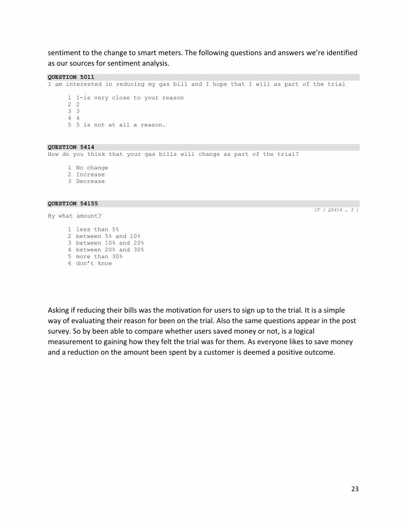
The responders to the Gas survey pre-survey where 1365. Gas customers were asked simple

questions. The first question to chosen to be examined for sentiment analysis, was did

responders believe that been on the trial would teach them to reduce their gas bill.

Gas customers responded, 153 No, 1212 Yes, out of the 1365 responders.

Users where then asked, “How do you think that your gas bills will change as part of the trial?”,

they were given three options to choose from, “1 = No Change, 2 = Increase, 3 = Decrease”.

They responded with the following output: No change Increase Decrease 328 20 1017 (1017/1365)*100 = 75% responded that they believed their bill would be reduced. Which is a massive degree of expectation. Users of gas where then asked, was a reduction in their gas bill their main reason for taken part in the trial, they responded: Main Reason Strong reason Good reason Medium Reason Not monetary 1064 226 38 11 26 Out of the 1365 responders, 77% said it was the main reason for participating in the trial was to reduce their gas bill. If we combine the values given for Main Reason + Strong reason + Good reason groups, which comes to 1328 responders, this is 97% of responders took part in the trial to save on their gas bills. Indicating that our logic of users participating in the trial to save on their gas bill as an excellent choice for sentiment analysis. Users where than asked: By what amount did they thnk they would save due to the trial? 1 less than 5% 2 between 5% and 10% 3 between 10% and 20% 4 between 20% and 30% 5 more than 30% 6 don’t know They responded:

33

<5% 5% - 10% 10%-20% 20% - 30% > 30% Don't Know NA's 97 433 278 60 18 131 348

7% of responders felt they would save less than 5% on their gas bill, 32% of responders felt they would save less than 5-10% on their gas bill, 20% of responders felt they would save less than 10-20% on their gas bill 4% of responders felt they would save less than 20- 30% on their gas bill. These categories represent the whole population of this trial, for participating in regard to how much they believe their bill will reduce. From above we can see 63% of responders felt they would save from 30% down on their gas bill. The post survey results are as follows to the same questions In the post survey, there was a reduction in respondents, 1233 responded to the post survey trial. (1365 – 1233) = 132, (132/1365) *100 = 9.67, this is a reduction of 10% in respondents. This resulted in higher NA’s and also the person who completed the first survey was not responding. However, when competing the post survey, those been questioned were only continued to be surveyed if they also and responsibility for the bill. For this reason we believe the data to be valid. Users where asked, did they believe their gas bills had changed as a result of the trial, they responded: Strongly Agree 85 Agree 418 No Change 234

Disagree 34 Strongly Disagree 19 Don't Know 16 NA's 417

We can see that from Strongly agree is 85 out of a total population of 1233, is 7%, but those in the who "agree" a group are 418, which is 33% of the total population and no change of 18% recorded from the total population. Interestingly if we combine those who disagree, strongly disagreed and the don’t knows, they only total 6% of the total population, as opposed to 40% who believe there has been a positive change for them moving to smart meters ( a reduction in their bill). However, we need to know more than that. What we know so far is, we can rule out a neutral effect from this point due to the fact 40% of the population had a positive change is greater than the 18% who believed they'd no change. If we add the Disagrees and Don’t Knows (6%) to the No Change groups, we get a total of 24%(negative) Versus 40% (positive). Initially moving to smart meters looks like a positive effect. When asked in the post survey by how much they believed their bills had reduced by, the

34

response from responders was:

<5% 82

5 - 10% 255

10 - 20% 126

20 - 30% 44

> 30% 18

Don't Knows 31

NA's 667

Out of the total population, 7% felt it reduced by 5%, 20% felt it reduced by 5-10%, 10% felt it had reduced by 10-20%, 4% felt it had reduced by 20-30%, 1% believing it had reduced by over 30%. In total 42% of the total population had responded to saving on their gas bill with the move to smart metering. This is quite a high rate of success when we acknowledge the NA’s, which now total for 54% of the population. If we remove the NA’s from this query and use only responders as the sample of the population (556 total responders), if we test again to see how many of the population felt their gas bill had reduced we get (525 responders had a reduction), this is 94% of the sample population. Felt they had save money by moving to smart meters. This is an extremely positive score. To confirm this the following analysis was ran on the following question which occurred in the post-gas-survey, Question 5500, And did your bill reduce to the degree that you expected? To which the resulting response was: PostSent$Q5500 = PostSent$Q5500.And.did.your.bill.reduce.to.the.degree.that.you.expected. > PostSent$Q5500 = factor(PostSent$Q5500, levels = c(1,2), labels = c("Yes", "No")) > summary(PostSent$Q5500) Yes No NA's 386 117 720

386 positive answers out of 1233 respondents, is 31% of the total population, though if we break that down to a sample set and concentrate on only those who responded answers (503 responders), 386 + 117 = 503, (386/503) *100 = 76% felt a positive effect in moving to smart meters of the sample group. Which is in line with the pre-survey of 97% who expected to make savings on their gas bills, resulting in a positive effect from them moving to smart meters.

35

Electricity customers who moved to smart meters was conducted using the KDD process and the same data selection, data pre-processing and transformation was applied. The pre-electric survey had 4232 observations(responders)and 144 variables(questions). Asked if participating in the trial would result in a reduction in their electric bill, the responded 368 No (9% of the total population) and 3864 Yes (91% of the total population). When asked more specifically whether their electric bill would have no change, increase or decrease, respondents replied as follows, No change Increase Decrease 778 37 3417

This represents 81% of the total population believe their electric bill would be reduced. When those been surveyed were asked by what percentage they believe their electric bill would be reduced, they responded, <5% 5% - 10% 10%-20% 20% - 30% > 30% Don't Know NA's 316 1240 1016 341 125 379 815

By adding the <5% groups up to >30% groups of the population, 71% of the total population expected their electric bill to decrease from less than 5% to over 30%. These results from the pre-electric survey are then compared to the post-electric survey. The post electric post-survey had 3423 observations, which is a decrease of 809 respondents this is a reduction of 19% in respondents. This resulted in as in the Gas-post-survey higher NA’s and also the person who completed the first survey was not responding. However, when competing the post survey, those been questioned were only continued to be surveyed if they also and responsibility for the bill. For this reason, we believe the data to be valid. For the question of whether their bills did decrease or increase as they hoped, the following question was asked and the output was as follows, summary(PostSentElect$Question.5414)

Decreased a lot 319

Decreased somewhat 1440

No change 732

Increased somewhat 134

Increased a lot 29

NA's 769

We can see from the above output that 51% of the total population felt they had a decrease in their electric bill, which indicates a positive result in the change to smart electric meters for these customers. If we use a sample of the population, removing the NA's, creating a sample population of 2654, (1759/2654) *100 = 67% of the sample agree their electric bill was reduced, this is a clear indication of a positive result in electric customers moving to smart meters.

36

Customers where then asked to give how much in percentage measurement, that they felt their electric bill had decreased, they responded, summary(PostSentElect$Question.54141) <5% 5% - 10% 10%-20% 20% - 30% > 30% Don't Know NA's 356 700 376 113 67 310 1501

This shows that of the total population, if we add less than 5% to greater than 30%, this shows that, (1612/3423) *100 = 47% believe that they had a reduction on their electric bill. If we ignore the NA's and use the total respondents as our sample group, that percentage figure rises to, (1612/1922) * 100 = 84% believe they saved by using to smart meters on their electric bill. Based on the data available, we can see very clearly that the change to smart meters made residential customers of both gas and electric feel they have saved on their utility bill, thus the sentiment of using smart meters for a utility services in these cases, is positive. There is an effect on users moving to smart meters and that effect is a positive effect. Users participated in the trial believing they can save money and they felt this was achieved.

Sentiment Analysis Conclusion:

Recall: The Null hypothesis was that gas customers would feel no change moving to smart meters. The Alternative was that there would be an effect on customers who changed. In this case as the answer is the same for both gas and electric customers, we can reject the null and fail to reject the alternative hypothesis, Simply put moving to smart meters had a positive effect on responders.

37

Data Usage

Selecting the Usage data

The data for usage of customers of Bord Gais and Electric Ireland customers was received as

outlined above in in the data dictionary in this report. As step 1 of KDD dictates, we need to

have data and understand it. This stage was reasonably simple; we already knew the data we

were going to use was in the files and we knew it’s format and how it was recorded. Data had

three columns, ID, DT and Usage. The usage was collected at 30 min intervals and DT gave the

code of whether the usage occurred at day or night time. These files were imported as per all

CSV files in this project into R Studio.

Pre-processing the Usage data

Pre-processing the data, step 2 of the KDD process was very difficult in the instances of

examining the usage of both domestic gas and electric customers. The files were enormously

large in the case of Electric usage files and in Gas the files there was were of a high number of

files.

Initially the plan was to total usage of a unique ID (customer), whose data was collected over a

period of time at 30 Min intervals. For example, the first 48 rows of each file, was the 24hr

usage period of a customer. This is a lot of repetitive rows data, where only the usage and time

period was recorded.

The gas usage files came in 78 CSV files. We attempted to sum up the usage of each ID, so they

would only take up one row of data in each file. This was successful but only to a certain point,

as R Studio would run out of memory when trying to do this.

Similarly, the Electric usage files came in only 6 files (each file was a text file so had to be

converted into CSV and also headers were missing) with all files over 400,000 KB. When we

attempted to sum up the usage by ID and merge the files together, R Studio ran out of memory

again before the computation and merging of the files was complete.

Another method of totalling usage by ID and merging the files was required. After some

research, PowerShell was chosen to attempt to compute the usage and merge the files of the

electric customers. Thankfully PowerShell was able to complete the merging of the files. The

following command is an example of how the electric usage files were merged.

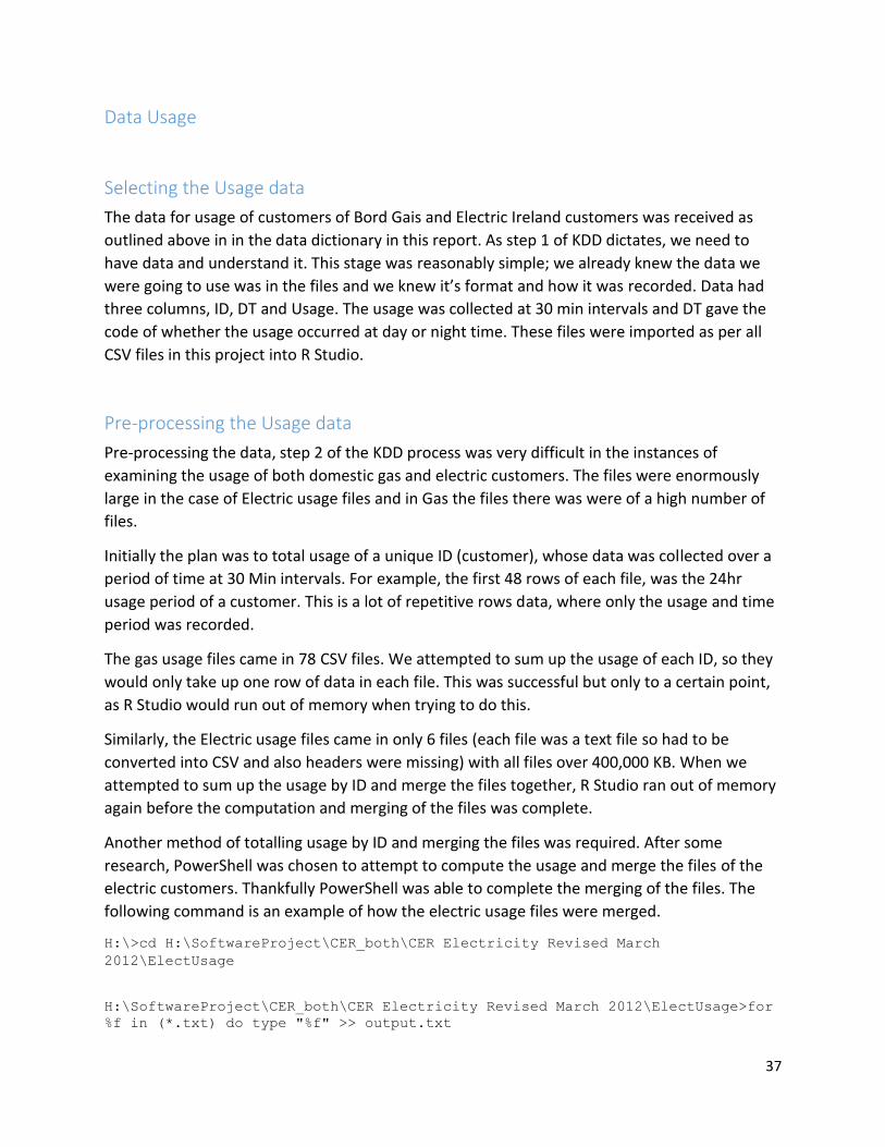
H:\>cd H:\SoftwareProject\CER_both\CER Electricity Revised March

2012\ElectUsage

H:\SoftwareProject\CER_both\CER Electricity Revised March 2012\ElectUsage>for

%f in (*.txt) do type "%f" >> output.txt

38

H:\SoftwareProject\CER_both\CER Electricity Revised March

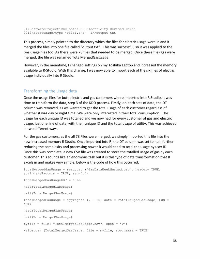
2012\ElectUsage>type "File1.txt" 1>>output.txt

This process, simply pointed to the directory which the files for electric usage were in and it

merged the files into one file called “output.txt”. This was successful, so it was applied to the

Gas usage files too. As there were 78 files that needed to be merged. Once these files gas were

merged, the file was renamed TotalMergedGasUsage.

However, in the meantime, I changed settings on my Toshiba Laptop and increased the memory

available to R-Studio. With this change, I was now able to import each of the six files of electric

usage individually into R Studio.

Transforming the Usage data

Once the usage files for both electric and gas customers where imported into R Studio, it was

time to transform the data, step 3 of the KDD process. Firstly, on both sets of data, the DT

column was removed, as we wanted to get the total usage of each customer regardless of

whether it was day or night time. We were only interested in their total consumption. The

usage for each unique ID was totalled and we now had for every customer of gas and electric

usage, just one line of data, with their unique ID and the total usage of utility. This was achieved

in two different ways.

For the gas customers, as the all 78 Files were merged, we simply imported this file into the

now increased memory R Studio. Once imported into R, the DT column was set to null, further

reducing the complexity and processing power R would need to total the usage by user ID.

Once this was complete, a new CSV file was created to store the totalled usage of gas by each

customer. This sounds like an enormous task but it is this type of data transformation that R

excels in and makes very simple, below is the code of how this occurred,

TotalMergedGasUsage = read.csv ("GasDataWeekMerged.csv", header= TRUE,

stringsAsFactors = TRUE, sep=",")

TotalMergedGasUsage$DT = NULL

head(TotalMergedGasUsage)

tail(TotalMergedGasUsage)

TotalMergedGasUsage = aggregate (. ~ ID, data = TotalMergedGasUsage, FUN =

sum)

head(TotalMergedGasUsage)

tail(TotalMergedGasUsage)

myfile = file( "TotalMergedGasUsage.csv", open = "w")

write.csv (TotalMergedGasUsage, file = myfile, row.names = TRUE)

39

close(myfile).

Transforming the electric files had a number of steps. The files were as text files and only file1

had headers. The decision was taken, to import the file, then create a CSV file from the text file,

this was done as follows below (using file 2, as example),

#File2

dir()

File2 = read.csv("File2.txt", header = FALSE, sep = " ")

head(File2)

myfile = file("File2.csv", open = "w")

write.csv(File2, file = myfile, row.names = TRUE)

close(myfile),

Once the file was a csv, it was checked against the text file to make sure the data was correct

and it was. Then the headers were added to the CSV file. The CSV file was then imported into R

Studio. Once in R the file and it’s headers, the aggregation of the usage by ID was performed,

the transformation to CSV and importation into R created an extra count variable X, this along

with the DT column were set to null and then the aggregation occurred, below is an example of

how this was achieved,

File2 = read.csv("File2.csv", header = TRUE, sep = ",")

head(File2)

File2$DT = NULL

File2$X=NULL

head(File2)

tail(File2)

#table the data

table(File2)

#once table format, now aggregate the Usage for each ID

File2ElectUsage = aggregate(. ~ ID, data=File2, FUN = sum).

This process was done for all the original electric usage files, each file had unique customer ID

numbers. No ID number was in multiple files, each file contained ID numbers unique to that file.

Once all the 6 individual files had been merged, so each row was a unique ID and that ID’s total

usage, the files were merged together.

40

We now had each user ID and their total usage for all gas and electric customers. As we had

gotten to know the data through the sentiment analysis and the initial KDD steps up to this

point, it was time to tackle the natural usage. Usage by their unique ID is not very useful. We

needed more variables to extract more knowledge from the totalled usage data. The variables

that were decided to be added to the totalled usage data, was the demographics of those been

surveyed. Added to the total merged data (id & usage) were the variables, Sex,

AgeOfResponder, who they live with, Adults in the house, Kids in the house, how many live in

the house and the number of bedrooms in the house. We used the ID variable to make sure

that the correct data correspondent to the correct data was merged.

The files which held the data now were called GasCustomersTotalById & ElectricityUsageModel.

These files were to be the basis for which our data mining would be based on.

Mining the Usage data

As mentioned previously separation of concern logic was applied during this project. The

totalled files and the merged additional variables were called GasCustomersTotalById &

ElectricityUsageModel . These files were imported into R. Once the data was in R, it was

decided that the ID and the count X variables were redundant to the data. We only wanted to

concentrate on the usage and these to variables did not contribute to that in any way.

The files GasCustomersTotalById & ElectricityUsageModel, were imported into R Studio, the

columns of ID AND x, new CSV files were created to hold the new dataset for both Gas and

Electric usage, these files were called GasCustomersClustering.csv &

ElectCustomersClustering.csv.

#import file that has all merged Gas data by id and their usage

BasicModel = read.csv("GasCustomersTotalById.csv", header = TRUE, sep = ",")

#check the attributes names on file

names(BasicModel)

#set what we don't need to 0

BasicModel$X=NULL

BasicModel$ID=NULL

#check attributes are now correct

names(BasicModel)

#get initial viisual of the data and the clusters

plot(BasicModel)

41

#save this as new file for clusterting

GasCustomersClustering.csv = BasicModel

myfile = file("GasCustomersClustering.csv", open = "w")

write.csv(GasCustomersClustering.csv, file = myfile,row.names = TRUE)

close(myfile)

The cluster analysis was performed in both R Studio and Weka. We gained an initial inference

by summarising each variable in R. We ran the clustering algorithm in R Studio for both gas and

electric customers.

In the case of the gas clustering, we imported the file GasCustomersClustering.csv, into R. We

then ran the following code (other values were used for k, but settled on 8 to avoid over and

under fitting). The following code was ran to run the cluster analysis in R.

#save this as new file for clusterting

GasCustomersClustering.csv = BasicModel

myfile = file("GasCustomersClustering.csv", open = "w")

write.csv(GasCustomersClustering.csv, file = myfile,row.names = TRUE)

close(myfile)

#now import that file

#to begin clustering analysis

ClusteringGas = read.csv("GasCustomersClustering.csv", header = TRUE, sep =

",")

#check attributes correct

names(ClusteringGas)

#get data summary

summary(ClusteringGas)

#get inital visual of the data

plot(ClusteringGas, main = " Gas Clusrering Analysis in R ")

kmeans.result = kmeans(ClusteringGas,8)

kmeans.result

42

Which resulted in the following output,

ithin cluster sum of squares by cluster:

[1] 458228719 476234589 2833591615 1232673650 776710148 441192325 479360

050 283223652

(between_SS / total_SS = 95.7 %)

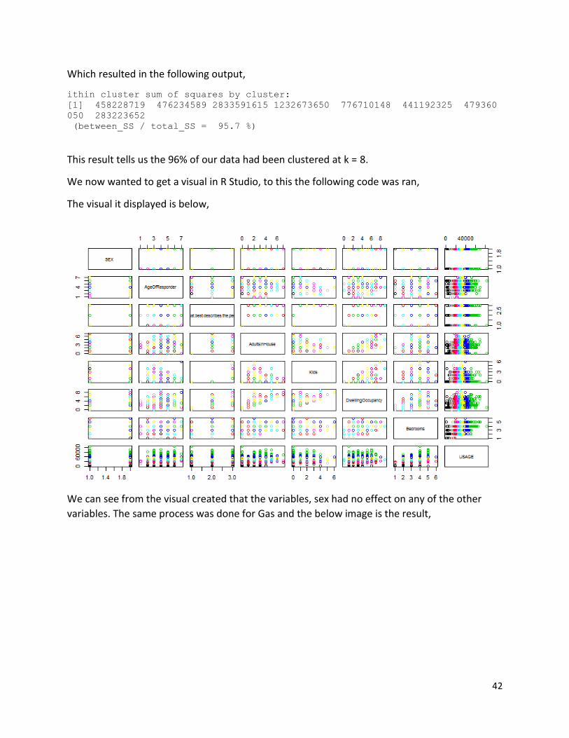
This result tells us the 96% of our data had been clustered at k = 8.

We now wanted to get a visual in R Studio, to this the following code was ran,

The visual it displayed is below,

We can see from the visual created that the variables, sex had no effect on any of the other

variables. The same process was done for Gas and the below image is the result,

43

44

Weka Clustering Visuals: Gas,

45

Electric Weka Cluster Visuals

We can the similarities between the tests run in R and Weka.

By performing the cluster analysis, we got a good eyeball test of the data and what may or may

not interact with each other. We can clearly see, that sex has no interaction with any variables.

From this point on, we can see there is no reason to include sex in our data mining process. We

can also see that who you live with interacts with usage as expected, as those that live alone

use less than the other two groups of groups (family units).

Just from this initial clustering we can see that Kids, Adults, number of bedrooms and house

occupancy have large interactions with usage. We can see this very clearly. The next step is to

46

classify and map the outcomes of these clustering’s. We want to extract more knowledge. To

do this we used decision trees to map this process.

Recall we are interested in usage of respondents, that is the goal of this project. The variables

chosen have a strong interaction with usage, we can see this from the clustering graphs, this

testifies to our knowledge and understanding of the data, that our choice of variables at this

stage is correct. We are know going to take out age of the responder

For creating the trees, we used Weka. To create a tree, we had to import the CSV files into

Weka, we had to filter the files from Numeric to Nominal, as in the current format, we would

not be able to create the tree we wanted. We want to run the J48 tree model on the data. Once

the files are imported into Weka, we need to first apply the filter, we do this by clicking on the

Choose tab, which gives us a drop down menu, which we then select the following, filters,

unsupervised, attributes, numeric to nominal, then click on apply button. Once this has been

done, we then click on the Classify tab. Once in the Classify window, we click the "Use training

set" option, then click on the Choose tab in this window, on the drop down list, click on Tress

and select J48 option, once we have done this, we click the start button in the Classify window.

This resulted in the following results,

ElectCustomersClustering = tree size = Number of Leaves :656, Size of the tree : 874

GasCustomersClustering = tree size = Number of Leaves : 418, Size of the tree : 551

As we can see the trees are too big to be fitted in this report, there is an example of the gas

tree above, as that was the smallest tree. Even though the tree is large, we can actually follow

in down the levels and get an outcome of usage for variables that are met.

47

To reduce complexity, it was decided that age of responder was not relevant, as again we are only

interested in the usage and age can be seen from the cluster analysis to be consistent across the age

groups, with little difference between the age groups. It was also decided to drop the variable who you

live with, as again the make up of those living in a dwelling whether they are a family etc was not

relevant to data usage. What was relevant to data usage was Adults, Kids, Dwelling occupancy and

Bedrooms in a dwelling. A new CSV files were created for both gas and electric customers, wth those

variables removed.

A test file was created for the purposes of this document to show a clearer path along the tree

structure. This was done for data reduction and to prune what variables we already knew had no effect

on usage. This was performed on the electric data.

Number of Leaves :45, Size of the tree: 53.

We will see the electric tree above for the tree usage file, we can follow down by number of people, to

number of bedrooms and we get a Usage amount that is associated with those variables.

This may seem an unusual way on classifying how to get natural usage but that is not the goal here. As

creating the tree is unsupervised, we are looking to gain understanding. The goal was for the tree

algorithm in Weka to return data to us, that we can understand and follow. It gives us more

understanding of the data as well as classification. Weka creates and returns a tree with 0.25

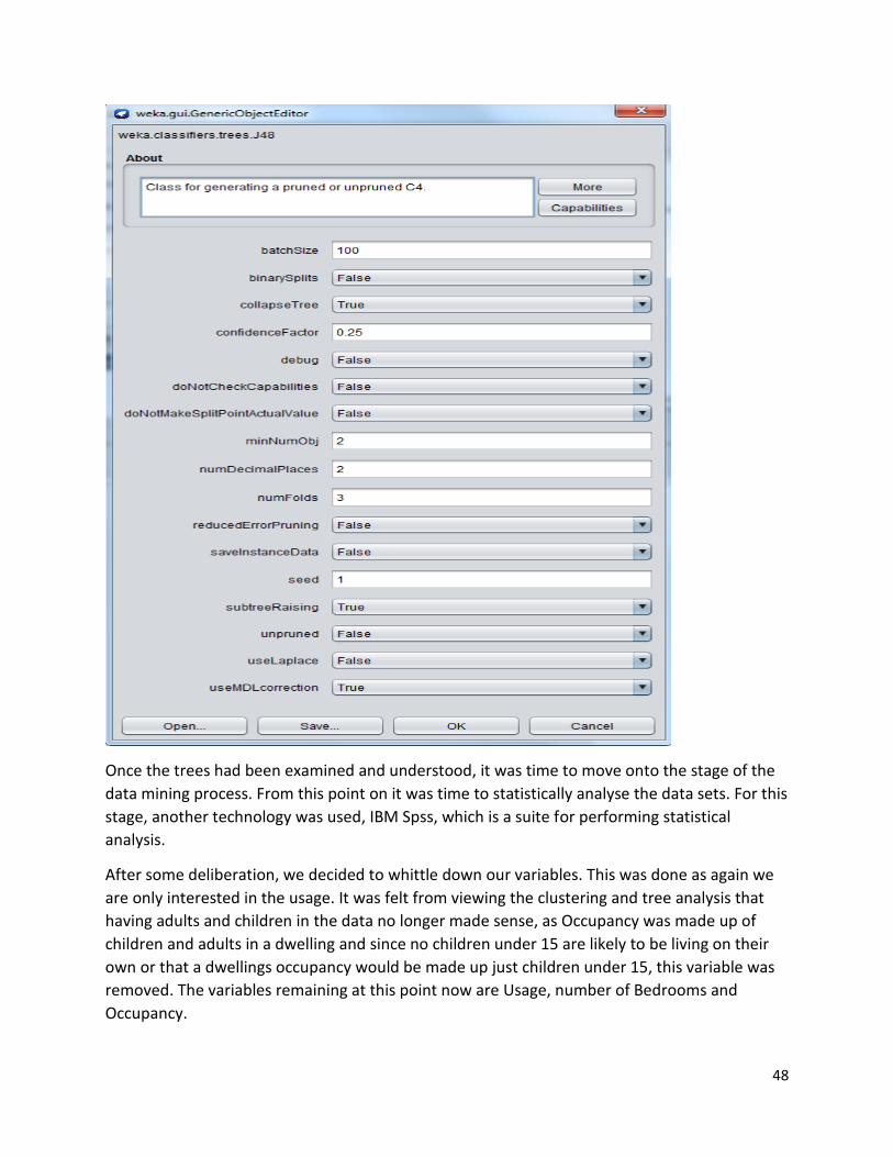
confidence, meaning that there is a 75% chance that not all variables have been classified. Below is the

settings of the Weka tree classification algorithm.

48

Once the trees had been examined and understood, it was time to move onto the stage of the

data mining process. From this point on it was time to statistically analyse the data sets. For this

stage, another technology was used, IBM Spss, which is a suite for performing statistical

analysis.

After some deliberation, we decided to whittle down our variables. This was done as again we

are only interested in the usage. It was felt from viewing the clustering and tree analysis that

having adults and children in the data no longer made sense, as Occupancy was made up of

children and adults in a dwelling and since no children under 15 are likely to be living on their

own or that a dwellings occupancy would be made up just children under 15, this variable was

removed. The variables remaining at this point now are Usage, number of Bedrooms and

Occupancy.

49

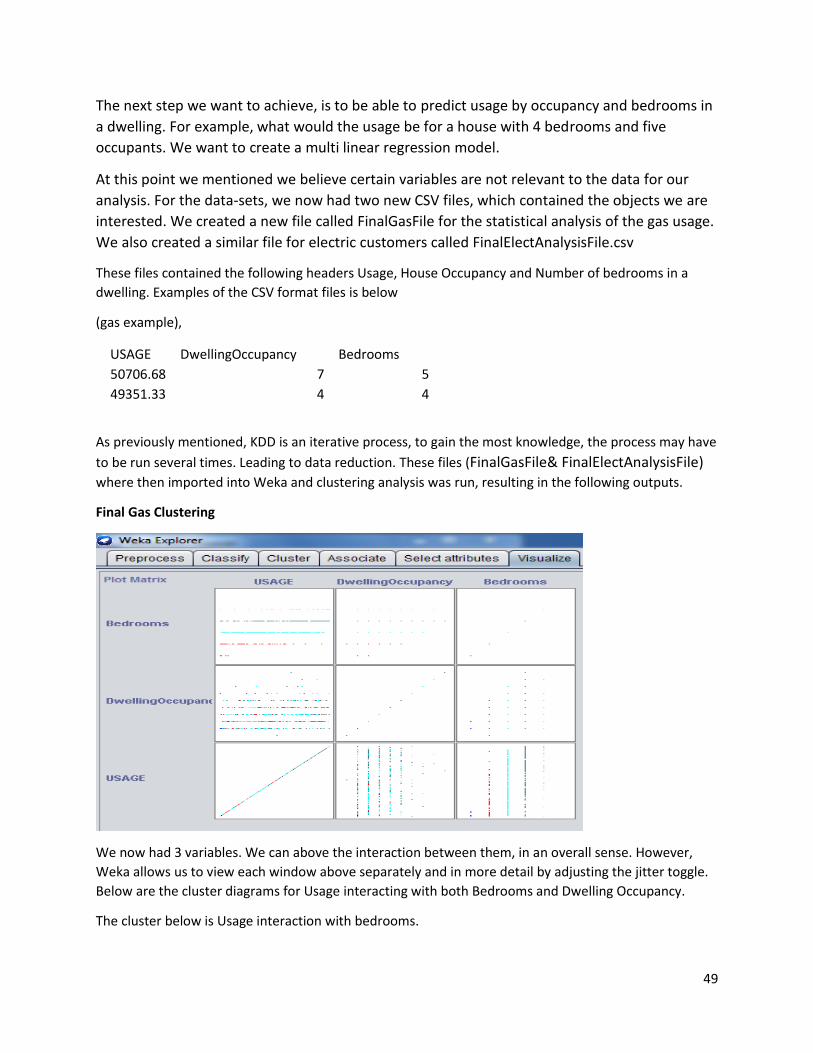
The next step we want to achieve, is to be able to predict usage by occupancy and bedrooms in

a dwelling. For example, what would the usage be for a house with 4 bedrooms and five

occupants. We want to create a multi linear regression model.

At this point we mentioned we believe certain variables are not relevant to the data for our

analysis. For the data-sets, we now had two new CSV files, which contained the objects we are

interested. We created a new file called FinalGasFile for the statistical analysis of the gas usage.

We also created a similar file for electric customers called FinalElectAnalysisFile.csv

These files contained the following headers Usage, House Occupancy and Number of bedrooms in a

dwelling. Examples of the CSV format files is below

(gas example),

USAGE DwellingOccupancy Bedrooms

50706.68 7 5

49351.33 4 4

As previously mentioned, KDD is an iterative process, to gain the most knowledge, the process may have

to be run several times. Leading to data reduction. These files (FinalGasFile& FinalElectAnalysisFile) where then imported into Weka and clustering analysis was run, resulting in the following outputs.

Final Gas Clustering

We now had 3 variables. We can above the interaction between them, in an overall sense. However,

Weka allows us to view each window above separately and in more detail by adjusting the jitter toggle.

Below are the cluster diagrams for Usage interacting with both Bedrooms and Dwelling Occupancy.

The cluster below is Usage interaction with bedrooms.

50

Bedrooms are on the y axis (to the left), we can see the range goes from 1 bedroom up to six. This

means within this data-set the least number of bedrooms is one and the maximum is 6. From the

dispersion of the data we can see that majority of Usage occurred by dwellings with three to four

bedrooms.

51

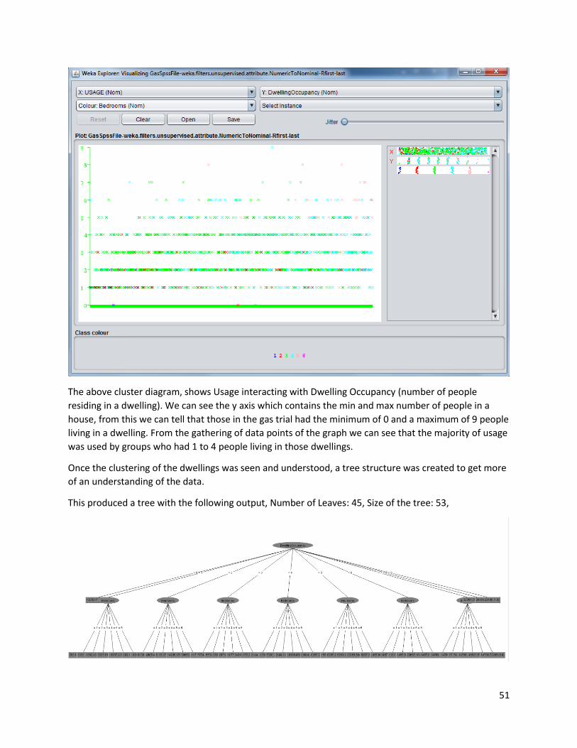
The above cluster diagram, shows Usage interacting with Dwelling Occupancy (number of people

residing in a dwelling). We can see the y axis which contains the min and max number of people in a

house, from this we can tell that those in the gas trial had the minimum of 0 and a maximum of 9 people

living in a dwelling. From the gathering of data points of the graph we can see that the majority of usage

was used by groups who had 1 to 4 people living in those dwellings.

Once the clustering of the dwellings was seen and understood, a tree structure was created to get more

of an understanding of the data.

This produced a tree with the following output, Number of Leaves: 45, Size of the tree: 53,

52

We can now follow the tree from number of people in a dwelling through to bedrooms to the usage.

The classification has been achieved, we can now use the tree as a flow chart to see if x amount of

people living in a dwelling has x amount of bedrooms, we know have all the usage options for them

classified.

Final Electric Clustering

Below is the overall clustering view of the three variables we are concentrating on for Electric usage,

which are the same as Gas usage, Usage, Dwelling Occupancy and Bedrooms.

As per the Gas usage clustering we will now see how the usage of Electric customers interacts with

Bedrooms and house occupancy.

53

Below is the cluster analysis from Weka which shows the interaction between Usage and Bedrooms.

Again we can see the min number of bedrooms in a dwelling is 1 and the max is 6. We can see the

majority of usage again occurs between dwellings that have 3 to 4 bedrooms.

54

Now we will check the interaction between Usage and Occupancy of a dwelling.

From the above graph of Usage v Occupancy we can see that the minimum occupant of a dwelling is 0

but the maximum is 12 (0 we are taking to mean the house is not occupied). We can also see that the

majority of usage occurs for dwellings that have between 2 to 4 occupants.

Now we will run the decision tree on the electric data set. We ran the decision tree in Weka and it

retuned a tree of, Number of Leaves :52, Size of the tree:61.

We can now follow the tree from dwelling occupancy to number of bedrooms to usage, this data-set has

now been classified.

55

Now that we have a good visual understanding and classification of these two data-sets, we

would now like to create a linear regression model. The purpose of a linear regression model is

predictions.

The data that makes up both Final files we are working on, have been drastically change from

the beginning of this process. From over a hundred variables, we’re down to just three now,

Usage, Dwelling Occupancy and Bedrooms. We now want to create a linear regression model

which will enable us to predict the amount of gas needed to supply a dwelling by the number of

people and bedrooms associated with said dwelling.

The formula for linear regression is: Y=a+Bx.

A linear model used one variable to predict an outcome.

The formula for multi linear regression is Y=a+Bx+Bx

A multi linear model uses more than one variable to predict an outcome

We can perform the multi linear regression in both R and IDM Spss. We will do this as it would

be interesting to compare these results and also for testing purposes.

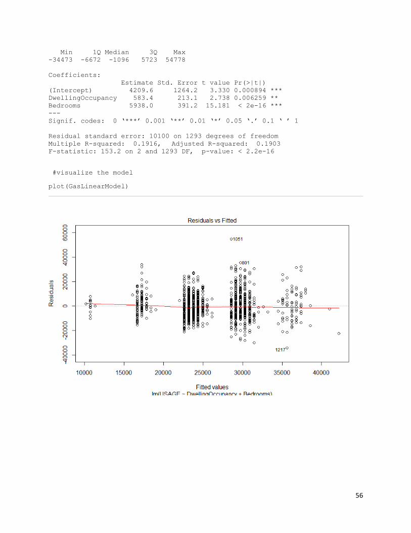
Firstly, in R studio we import the CSV file holding our data, install the packages and libraries, set

our working directory and then run the multi linear regression. The file has been labelled

GasLinearModel in the gas script, below is the code that creates the model and returns our

outputs.

LinearModel = read.csv("FinalGasFile.csv", header = TRUE, sep = ",")

#show our variables

> names(GasLinearModel)

"USAGE" “DwellingOccupancy" "Bedrooms"

#build gas mlr model

GasLinearModel<- lm( USAGE ~ DwellingOccupancy + Bedrooms ,

data=GasLinearModel)

#DISPLAY Model

Call:

lm(formula = USAGE ~ DwellingOccupancy + Bedrooms, data = GasLinearModel)

Coefficients:

(Intercept) DwellingOccupancy Bedrooms

4209.6 583.4 5938.0

#Multi Linear Gas Model Results

summary(GasLinearModel)

Call:

lm(formula = USAGE ~ DwellingOccupancy + Bedrooms, data = GasLinearModel)

Residuals:

56

Min 1Q Median 3Q Max

-34473 -6672 -1096 5723 54778

Coefficients:

Estimate Std. Error t value Pr(>|t|)

(Intercept) 4209.6 1264.2 3.330 0.000894 ***

DwellingOccupancy 583.4 213.1 2.738 0.006259 **

Bedrooms 5938.0 391.2 15.181 < 2e-16 ***

---

Signif. codes: 0 ‘***’ 0.001 ‘**’ 0.01 ‘*’ 0.05 ‘.’ 0.1 ‘ ’ 1

Residual standard error: 10100 on 1293 degrees of freedom

Multiple R-squared: 0.1916, Adjusted R-squared: 0.1903

F-statistic: 153.2 on 2 and 1293 DF, p-value: < 2.2e-16

#visualize the model

plot(GasLinearModel)

57

A Q-Q Plot is used to see if data is normal, if the data is close to the line generally we say the

data is normal. We don’t need to check for normality when doing regression but it is a good

visual to view. For instance, our data is mostly normal but it veers away from the central line at

head of the line and at the foot of the line we can see an outlier. These make the data not

normal.

58

We can see just through an eyeball test that 25000 is our central point and the majority of our

data falls within two places of the central line. Which we hope for.

59

In Spss we load the CSV file in, we then select Analyse tab and scroll down the list that creates

and choose Regression, from the submenu of Regression we choose Linear, which then

populates a window Linear regression window, we add usage as the dependent variable and

Dwelling Occupancy and Bedrooms as the independent variables and click ok, thisreturns us the

following outputs……which we can see are the same as in R. by doing these checks, we are

actually testing the consistency of our work and that the utputs are correct and reliable.

60

Model Summary

Model R R Square

Adjusted R

Square

Std. Error of the

Estimate

1 .438a .192 .190

10103.9834200

00

a. Predictors: (Constant), Bedrooms, DwellingOccupancy

The above table is the result of testing our model. It reveals we our model is just below medium

in strength, R = .438. This may seem low but if a utility can get 44% prediction of usage of

people in an area or neighborhood from this model or even in general that would go a long way

to planning their output and services. It may even be incorporated into their existing model.

Electricity Linear Model code and visuals, #create model

> ElectMLR<- lm( USAGE ~ House.Ocupancy + Bedrooms , data=ElectUsage)

> #view model results

> ElectMLR

Call:

lm(formula = USAGE ~ House.Ocupancy + Bedrooms, data = ElectUsage)

Coefficients:

(Intercept) House.Ocupancy Bedrooms

76.71 56.72 64.01

We did the same process for the Elect again both R and Spss, are the same values, Showing us testing in both confirms our value output.

Coefficientsa

Model

Unstandardized Coefficients

Standardized

Coefficients

t Sig.

95.0% Confidence Interval for B

B Std. Error Beta

Lower Bound

Upper Bound

1 (Constant) 76.705 15.409 4.978 0.000 46.496 106.914

House.Ocupancy 56.723 2.278 0.361 24.895 0.000 52.256 61.190

Bedrooms 64.013 4.617 0.201 13.864 0.000 54.961 73.065

a. Dependent Variable: USAGE

61

Model Summary

Model R R Square

Adjusted R

Square

Std. Error of the

Estimate

1 .471a .222 .222 237.618413

a. Predictors: (Constant), Bedrooms, House.Ocupancy

We have a slightly stronger model in Electricity than in Gas but not by much, we have a prediction accuracy of 48%

Evaluating the Usage data

The process of data mining the usage variable in our project is long and produces results in the

mid 40% range. This as mentioned may not seem huge but if these models can be used by a

utility company to even reduce their output by 1% it would be massively beneficial. As if a

company is turning over millions even billions per year a saving of 1% would be of enormous

benefit to them.

The outset of this project was to study the natural usage and somehow crate a predictive model

for usage. We’ve done this and this was achieved by following the KDD process.

Project conclusion

From our analysis we can see that responders were happy with the change to smart meters. If we were

to advise a utility company on rolling out such a product, we would highly recommend this.

In terms of usage we feel a utility company could gain some use and knowledge from our model and the

process we went through in whittling down the variables of interest. A small change to a large revenue

company can result in significant savings.

I ran the model on other variables and sent this information to the CSO, with the extra variables there

was very little difference to having the added variables and just using the three that we did in the end.

62

Overall Project Reflection

It would have been brilliant for analysis reasons to have had data relating before the smart meter trial. I

believe a better model could have been made with this data. It would have given us a bench mark to

work off.

We ran the same steps again with the variables we dismissed after the tree stage of our data mining

process, the following result of the model and correlations can be seen below for both Gas and Electric

responders,

Correlations

USAGE AdultsInHouse Kids

DwellingOccupa

ncy Bedrooms

Pearson Correlation USAGE 1.000 .263 .051 .218 .432

AdultsInHouse .263 1.000 .048 .734 .322

Kids .051 .048 1.000 .692 .186

DwellingOccupancy .218 .734 .692 1.000 .356

Bedrooms .432 .322 .186 .356 1.000

Sig. (1-tailed) USAGE . .000 .034 .000 .000

AdultsInHouse .000 . .042 .000 .000

Kids .034 .042 . .000 .000

DwellingOccupancy .000 .000 .000 . .000

Bedrooms .000 .000 .000 .000 .

N USAGE 1296 1296 1296 1296 1296

AdultsInHouse 1296 1296 1296 1296 1296

Kids 1296 1296 1296 1296 1296

DwellingOccupancy 1296 1296 1296 1296 1296

Bedrooms 1296 1296 1296 1296 1296

Model Summaryb

Model R R Square

Adjusted R

Square

Std. Error of the

Estimate

1 .453a .205 .203

10026.4826600

00

a. Predictors: (Constant), Bedrooms, Kids, AdultsInHouse,

DwellingOccupancy

b. Dependent Variable: USAGE

63

The Gas model only increased by 1%, which makes the decision valid for removing them to lessen

complexity and our decision process for removing them also.

We also ran the Electricity model again but with added variables,

Variables Entered/Removeda

Model

Variables

Entered

Variables

Removed Method

1 Bedrooms,

AGE, Sex,

ADULTS, KIDS,

PeopleYouLive

Withb

. Enter

a. Dependent Variable: USAGE

b. Tolerance = .000 limit reached.

This model actually increased the R value, as can be seen below

Model Summaryb

Model R R Square

Adjusted R

Square

Std. Error of the

Estimate

1 .479a .230 .229 236.577069

a. Predictors: (Constant), Bedrooms, AGE, Sex, ADULTS, KIDS,

PeopleYouLiveWith

b. Dependent Variable: USAGE

This actually increased to 48%. So in this case and on reflection it may have been wiser to have kept the

additional variables present on the multi linear regression. But at such a small increase in model %, we

feel we were justified in making them redundant during the process.

Testing

Testing was done throughout the process of the KDD model and testing our results in different

technologies. All tests proved to be successful as only minor discrepancies occurred in the technologies

results returned to us.

To some testing is not important in this type of project but I disagree. By constantly testing our results,

we can guarantee that we made the correct steps in each technology when analysing our data.

64

Monthly Project Journals

Reflective Journal

Student name: Damien Grouse x13114328

Programme : BSc in Computing, Data Analytics Stream

Month: 12th September - 07th October 2016

Introduction

I'm a fourth year student, attending the National College of Ireland and this is my reflective

journal charting my progress for my final year project. I want to look back on this journal after

and during my project, to use it as a tool to keep me focused but also as a semi-informal

document I can read and recall what I went through to complete my project. So I intend to

write it in a somewhat informal style.

My fourth year in college began on the 12th of September 2016 and I knew I would have a

major final year project to do. I chose to specialize in Data Analytics for my final year. I've a

keen interest in Databases but particularly Statistics, so that was my reason for choosing that

particular stream. So during the summer I was thinking of ideas for my final project. I used my

time on my work placement to formulate and float ideas to people who work in the IT industry.

I made a point of having at least half a dozen ideas on which to do my final project on, by the

time I returned to college.

My Achievements

This month, I had to whittle down my half a dozen ideas down to just one.

12/09/2016 - 17/09/2016

When I returned to college I had a number of ideas of what to do my final year project on. I

decided that I would use this week to get my ideas down to just one. I did this by floating my

ideas past my lecturers and fellow classmates. As I am specializing in Data Analytics, it made

sense to do my project in this field. I also made contact with the CSO (Central Statistics Office),

for general information and on the off chance they may have data sets available for me to use

and hopefully to do a project for them. As they are the best people to contact regarding

statistics in the country. By the end of the week I was down to the following three ideas,

65

build an application that allowed for real time data visualization for a business's needs (sales,

stock, staffing levels etc)

devise a retail rental pricing model, using heat maps, were rent is set on the amount of foot

traffic through areas of shopping centres ( most foot traffic = bigger rent)

to take a real and published data set and look for new trends

18/09/2016 - 24/09/2016

I have decided to go with my idea of getting a real data sets and to look for new trends. There

were several reasons behind this. The primary reason was, I heard back from the CSO ( John

Dunne emailed me), pointing me in the direction of Smart Metering on dwellings(Electric and

Gas) and a study previously done. This could give me access to real data, that is clean and

reliable. He also said " I would be interested in a project that took the smart metering data,

clustered households naturally based on usage patterns and then tried to describe them

based on usage patterns and information collected in the accompanying survey, I think

such a project would be very interesting". So I am going to use this direction as the core

study behind my project.

25/09/2016 : 01/10/2016

I had to apply to ISSDA and UCD to get access to the data. I sent an email and filled in an

application form. I am anxious to receive this as next week I have to present my idea to

lecturers so I can get their approval to proceed with my topic for my final year project.

02/10/2016 : 08/10/2016

I received the data from the ISSDA and UCD (there is a lot). I presented my case for my final

year project and I got an enthusiastic response from the three lecturer panel and some good

ideas also. They were very supportive in my choice of project. I've to wait till next week to find

out who is going to be my project Supervisor. So when that happens, my project will really

begin.

My Reflection

I'm pleased with how I went through the process of deciding my final year project. I can write

and understand code(java) but I really do not enjoy it. It always seems like a chore to me. I've a

real interest in Databases and Analytics, these interests really shaped the kind of project I

wanted to do(plus I am specializing in Analytics, so it makes sense). I got great feedback from

my project proposal presentation, which made me feel very positive on my choice of project.

66

I was happy with the response I got from who I reached out to, the CSO and ISSDA and UCD in

particular. My project tutor Eamon Nolan, has been great too, he's accessible, concise and

forthright in his views and answers to what I ask him, which I like .

I've real data to work with, which I really wanted. I'm excited to learn who my Supervisor will be

and getting the real work started on my project over the next few weeks.

Going forward

It was mentioned to me during my proposal that it may take me at least a month to six weeks

for me to get a grasp and understanding of the data I'd been sent. So for now till next month

my aim is to do that and to create a good relationship with my Supervisor and to come up with

a plan for the remainder of my project, at least up in till Christmas and with an eye on planning

my project schedule into the new year. I'll also make sure I stay on top of my submissions.

Supervisor Meetings

N/A yet to be allocated my Supervisor

Date of Meeting:

Items discussed:

Action Items:

Reflective Journal


Program : BSc in Computing, Data Analytics Stream

Month: 8th October - 4th November 2016

Introduction

This month has been bit of a nightmare in terms of time management. I've so many projects,

CA's on-top of learning new course work, that I've got very little done on my project that can be

measured in terms of work achieved.

My Achievements

This month I have made progress but not as much as I would have liked or maybe I am been too

hard on myself. Just currently I am feeling like I've a mountain to climb with all my course work

and with demands outside of college too. Plus I uploaded the wrong project proposal

document, so need to talk to Eamon about that, as it won't let me edit the submission, even

though it is still a live document.

67

I've been allocated Michael Bradford as my project supervisor. We were told that our

supervisors chose what projects and students they wanted to mentor. As many in our class

wanted Michael as their supervisor I drew some confidence that what I proposed he found

interesting and wanted to see.

I've met Michael a couple of times now and found him very easy to talk to and approachable.

He has a genuine interest in my project and I am looking forward to what advice he can give

me. I've set up a Github account and Michael has access to my project now. Initially we used

Dropbox but with the size of my project, I ran out of space quickly.

As I am learning as I go in terms of data analytics(R & Python languages etc), I'm getting to grips

with all the data I have and getting an understanding of it. As Michael advised me, I'm spending

the next few weeks(up till mid/end November) understanding the data and applying new

knowledge gained on my course to my project.

My Reflection

I've got my project supervisor. I am still getting to know my data and as that it not easily

quantifiable, in terms of effort applied, I was feeling I was not progressing much this month but

on writing this document I've realised I am progressing and that I knew it would take me a

couple of months to understand the data I have. So I am going to keep on going and try not to

be so hard on myself.

Going forward

I'm to have a more precise project plan to show Michael and get his opinion on it. He has told

me to relax and not be so hard on myself. That to see the bigger picture and that by

understanding all my data and having a clearer project plan, it will stand to me, when it comes

to querying the data and producing a strong project.

Supervisor Meetings

Michael Bradford is my Project Supervisor/Mentor.

We have met twice already, we have agreed to meet every two weeks on a Thursday.

Date of Meeting: 20/10/2016 & 03/11/2016

Items discussed: Initial meeting was a broad discussion of my project. Second meeting was a

discussion on my data and a general timeframe for my project was agreed. I've to bring an

exact schedule to our next meeting

Action Items: Have a specific project plan in terms of project milestones.

68

Reflective Journal



Month: 4th November - 9th December 2016

Introduction

This month has been and I can't believe I'm writing this, was even worse than last month. We

on the course have been totally screwed over time-wise and workload. We are struggling to

maintain any sort of standards we've set ourselves over the last three years in college. But by

the end of it, I have somehow managed to keep to all my deadlines and my midpoint has got

some positive feedback from my project mentor Michael Bradford considering where I was with

the whole college experience this semester.

My Achievements

This month at the start of it, we had come through a very tough time and it did not get any

easier this month, in fact it went up a few gears, in the words of Ron Burgundy…"That escalated

quickly".

We are to have our Technical report and our Mid-point presentation ready for the start of

December. However we also had a number of CA's, project submissions and the dates of these

kept changing, between students not having enough time and lecturers been off sick. These

issues caused delays and really piled on the workload to the end of the month and ranked up

the pressure.

By the middle of the month I was really stressed out and at this stage I was offered a full time

job and I nearly took it. As I've only few months left and I really do want my Honours Degree, I

turned it down. I don't want to create a glass ceiling for myself by not completing this year. I got

to admit though I was seriously thinking about leaving.

I obviously didn't take the job….I am writing this after all.

A major reason behind my staying on my course was my project mentor Michael Bradford. He

was a real calming influence for me. My head was all over the place. He spoke an awful lot of

sense to me and I am indebted to him for this.

I concentrated on updating my live documents after speaking to Michael, so my project

proposal and tech Spec documentation got pieces added to them. I then added these extra

features to my Technical report, along with additional information required for my technical

report. This really helped me get my mind back on track and cleared a lot of my project plan up

for me. I got that done on time and also my midpoint presentation.

69

Once the documentation was in order, I got down to the nitty-gritty of beginning to pre-process

and get to grips with the enormous amount of data I have. I've ran some summary queries on

the data. For my midpoint I am going to show my inference from two questions in the

sentiment survey. These two questions were answered by a total of 1365 residents surveyed.

So the information gathered and my inference was insightful. I used graphs to display my

findings, I then mapped both queries together to gain further insights. This is the KDD iterative

process I will be taking throughout my project, even is this just a sample version of it. My slides

are complete and I am ready to to my midpoint presentation.

My Reflection

Michael has been a great influence on me. We meet regularly and he's available also for when I

need to run anything by him, which is a great help. He really does help me stay on track and

challenge myself. But I got to admit, I nearly quit this month but glad I didn't.

Going forward

We've exams coming up, so I don't expect to get much more done on my project till they are

done towards the end of January. Once they are, I'll update my project plan and stick to it. I've

less modules next semester, so more time and with this I expect my project work to kick up a

few gears and for me to really start getting into it.

Supervisor Meetings


We have met four times this month. Date of Meeting: 8/11/2016 & 08/12/2016

Items discussed: Midpoint, documents and work life balance and not quitting to go working.

Action Items: all milestones met this semester and will evaluate new plan after my exams..

Reflective Journal



Month: 9th December 2016 - 5th January 2017

Introduction

This month has been manic. I'd to complete my mid-point project presentation.

My Achievements

70

I submitted my mid-point presentation. The presentation went as well as I could have hoped. I

was not really happy with it, as everything about my project this semester has felt rushed due

to the ridiculous workload we have. I managed to complete every element I was required to do.

I scored 67%, which works out at 16.75% out of a possible 25% of my project so far. So with a

bit more time next semester I hope to increase this grade.

My Reflection

I've not got any more work done on my project since my mid-point presentation, as I've been ill

and also preparing for my exams.

Going forward

Once my exams are over with, I believe we'll have two weeks off before the next semester

begins. I am going to take 3 to 4 days off after they are over. I will then come in to the library

and start working again on my project, get a head start on machine learning and data mining.

I'll also probably move all my data into an Sql database too.

Supervisor Meetings


We have met 3 times this month. We have every 2 weeks a scheduled meeting.

Michael is an excellent supervisor, he always has ideas to bounce off me and he listens and

advises me on my ideas too.

Items discussed: Midpoint, documents and going forward for next semester.

Action Items: get project back on track once exams and little break out of the way. Come up

with new project plan for semester 2.

Reflective Journal



Month: 7th Feb 2016 - 11th March 2017

Introduction

This month has been extremely busy….again…as we had some CA’s and Submissions to

complete.

My Achievements

Last month I began exploring the data, I’m almost finished this phase now and am moving onto

to targeting and removing the data that is not relevant to my project goals.

71

My Reflection

I feel really positive at the moment, my mentor says I am on schedule and I fell I made good

progress in understanding the data and I am now ready to move onto the next phase of my

project.

Going forward

I’ve cleaned the data and I am now targeting the data I require (KDD process), I expect to have

the majority of my data processing completed this month and should by the end of reading

week, have my sentiment analysis section of the project complete. Once I’ve done the practical

and technical elements of this, I will then begin to start my project submission document.

Supervisor Meetings


We now have a scheduled meeting every week (when either of us cannot make the meeting,

we acknowledge that, then rearrange.)

Items discussed: Michael has said I am on point to meet my project deadlines and I am looking

forward to showing him the completed sentiment analysis. Which will then leave me to focus

on the natural usage part of my project.

Action Items: to move onto the next phase of KDD and to begin gaining knowledge.

Reflective Journal



Month: 11th March 2017- 6th April2017

Introduction

This month by project took bit of a backseat, as I’d other CA’s and Projects and Submissions due

in my other subjects for this semester.

My Achievements

I’ve no finished half of my project, which was the Sentiment analysis. Which I am pleased with

my findings but I’d still rather be further along in my project, personally.

My Reflection

I’ve made progress, though not at the pace I was hoping to achieve. But I know many of my

class mates are still not even started, so I am taking some comfort in that. Though I am finding

72

this whole year very lonely. The guys I’d usually be with are on a different stream and I spend

most of my time on my own and I miss bouncing ideas around.

Going forward

Sentiment analysis is now done…so that’s half the project done and now it is in to the next

phase, studying the natural usage of the customers. The next two weeks I’ll chip away at the

project but my main focus is studying for my exams. But I know I’ll be on course to submit on

time.

Supervisor Meetings


We now have a scheduled meeting every week (when either of us cannot make the meeting,

we acknowledge that, then rearrange.)

I haven’t seen Michael as much as I’d have liked but that is not down to him or me, it’s the fact

that a few classes were rescheduled and this led to them colliding with our usual meeting time/

Action Items: begin KDD process on natural usage part of the project.

Images

All images were created by the author

Apart from Fig(4)

Which came from slides issued by Simon Caton, Lecturer of National College of Ireland, 2016.

Date post:	12-Mar-2018
Category:	Documents
Upload:	lekhanh
View:	216 times
Download:	1 times

A study of natural usage and sentiment analysis of ...trap.ncirl.ie/2660/1/damiengrouse.pdf · All...

Documents