HAL Id: hal-01150856https://hal.archives-ouvertes.fr/hal-01150856

Submitted on 12 May 2015

HAL is a multi-disciplinary open accessarchive for the deposit and dissemination of sci-entific research documents, whether they are pub-lished or not. The documents may come fromteaching and research institutions in France orabroad, or from public or private research centers.

L’archive ouverte pluridisciplinaire HAL, estdestinée au dépôt et à la diffusion de documentsscientifiques de niveau recherche, publiés ou non,émanant des établissements d’enseignement et derecherche français ou étrangers, des laboratoirespublics ou privés.

Copyright

A study of transverse cracking in laminates by the ThickLevel Set approach

Thibault Gorris, Paul-Émile Bernard, Laurent Stainier

To cite this version:Thibault Gorris, Paul-Émile Bernard, Laurent Stainier. A study of transverse cracking in lami-nates by the Thick Level Set approach. Mechanics of Materials, Elsevier, 2015, 90, pp.118-130.10.1016/j.mechmat.2015.05.003. hal-01150856

A study of transverse cracking in laminatesby the Thick Level Set approach

Thibault Gorrisa, Paul-Émile Bernardb, Laurent Stainiera,∗

aInstitut de Recherche en Génie Civil et Mécanique (GeM, UMR 6183 CNRS)École Centrale Nantes, 1 rue de la Noë, BP 92101, F-44321 Nantes, France

bInstitute of Mechanics, Materials and Civil Engineering (iMMC)Université catholique de Louvain, 4 ave. G. Lemaître, B-1348 Louvain-la-Neuve, Belgium

Abstract

In this paper, we present an analysis of the transverse cracking and interface failure process in-duced in layered materials (such as composite laminates) subjected to tensile loading, with a newlevel set based non-local modeling approach for damage growth (TLS: Thick Level Set). In par-ticular, a 2D finite element model is built to study damage in a cross-ply laminate. The studyaims at evaluating the capacity of the TLS method to predict evolution of damage at the ply level,including initiation, propagation, merging of cracks or delamination. We show how this numericalmodel is able to reproduce key features such as crack spacing saturation and other experimentalobservations.

Keywords: non-local damage, Thick Level Set, transverse cracking, composite laminates

1. Introduction

The appearance and development of transverse cracks in layered materials is an importantproblem in many fields of engineering, for example in composite laminates (Garret and Bailey,1977; Highsmith and Reifsnider, 1982; Manders et al., 1983), thin-films (Thouless et al., 1992),civil engineering (Hong et al., 1997), or geology (Price, 1966). It is well established that in thisconfiguration of layered materials, cracks tend to self-organize, with a spacing which is directlyrelated to the relative thickness of layers. Explanations for this phenomenon, based on shieldingeffects, have been proposed on the basis of fracture mechanics (e.g. Bai and Pollard, 1999; Baiet al., 2000). This type of analysis relies on the study of the effect of discrete cracks placed inelastic layers, and although it can explain why a given crack distribution is optimal or natural insome way, it cannot provide details on the process which would lead to this crack distribution.

Transverse microcracking and local delamination in fiber-reinforced composite laminates havebeen studied mainly within the framework of finite fracture mechanics. Analytical approacheshave been used for crack growth with energetic criteria that have allowed the definition of a largenumber of successful fracture models such as in Dvorak and Laws (1987), and others (Hashin,

∗Corresponding author: laurent.stainier@ec-nantes.fr

Preprint submitted to Mechanics of Materials May 11, 2015

1996; Nairn, 2000; Varna et al., 1999). Rebière and Gamby (2004) recently proposed an analyticalenergetic criterion for modeling crack initiation and propagation in the matrix as well as delamina-tion in cross-ply laminates. Alternatively, numerical models have been proposed to model matrixfracture, based on finite element approaches combined to bulk damage (Berthelot et al., 1996) orcohesive elements (Okabe et al., 2004). The meso-model developed by Ladevèze (Ladevèze andLubineau, 2001; Ladevèze et al., 2006) predicts damage evolution directly at the ply level. Dueto the variability of local material properties within the plies, the heterogeneity of mesoscopicstructures must be considered. Some authors introduced a statistical criterion in strength like inBerthelot and Le Corre (2000), or a statistical criterion in toughness as in Andersons et al. (2008).Numerical studies of the propagation of debonding at the tip of transverse cracks were also treatedby a variational approach to fracture (Baldelli et al., 2011).

Modeling the progressive degradation of materials from an initial undamaged state to totalfailure is still a challenge in computational mechanics. Damage models can be used to describethe initial degradation of mechanical properties, while fracture mechanics is well adapted to finalstages leading to fracture. The Thick Level Set (TLS) approach, proposed by Moës et al. (2011),allows for a seamless transition between damage and fracture, while providing the necessary reg-ularization in presence of softening.

In this paper, we present an analysis of the transverse cracking and interface failure processinduced in layered materials (such as composite laminates) subjected to tensile loading, using theTLS approach. The main aspects of this method will be presented in section 2. In section 3, a 2Dfinite element model is built to study damage in a cross-ply laminate. The study aims at evaluatingthe capacity of the TLS method to predict evolution of damage at the ply level, including initiation,propagation, merging of cracks or delamination. For this, we will start from undamaged (virgin)material with small but random variations of mechanical properties, and simulate the initiationand evolution of cracks. In section 4, we show how this numerical model is able to reproduce keyfeatures such as crack spacing saturation and other experimental observations. We also study theeffect of some algorithmic parameters involved in the TLS method. The paper closes with someconclusions and perspectives.

2. Thick Level Set (TLS) approach

2.1. Continuum damageOur objective in this work is to study the development of transverse cracks in layered materials,

starting from a virgin (crack-free) state. It is nowadays well established that continuum damagemodels (CDM) are appropriate to treat early stages of material degradation. Abundant literatureon CDM is available, which analysis is nonetheless beyond the scope of the present paper, and wewill simply refer the reader to Lemaître et al. (2009).

2.1.1. Local constitutive relationsWe will work under assumptions of linearized kinematics, and consider a simple elastic-

damage model described byσ = C(d) : ε (1)

2

where σ is the Cauchy stress tensor, ε the engineering strain tensor, and C(d) a fourth-orderelasticity tensor, function of the scalar damage variable d ∈ [0, 1]. The model can alternativelybe described in the framework of generalized standard materials (Halphen and Nguyen, 1975;Germain et al., 1983), by defining the free energy potential, a function of the material state ε, d:

W(ε, d) =12ε : C(d) : ε. (2)

This potential in turn allows to define thermodynamical forces conjugate to state variables ε andd:

σ =∂W∂ε

(ε, d) (3)

Y = −∂W∂d

(ε, d) (4)

It is easily verified that (3) is equivalent to (1). Relation (4) defines the energy release rate Y ,thermodynamically conjugate to damage d. The equation describing the evolution of damage isthen obtained through the dissipation potential ψ(Y):

d ∈ ∂Yψ(Y) (5)

where ∂Yψ denotes the sub-gradient of ψ(Y), a (potentially non-regular) convex function of Y .Following standard arguments, convexity of ψ(Y), combined to conditions ψ(0) = 0 and ψ(Y) ≥0∀Y , ensures positivity of the dissipation:

D = Yd ≥ 0. (6)

This formalism allows to simultaneously cover both rate-independent and rate-dependent damagemodels. Indeed, the rate-independent case corresponds to a lower semi-continuous dissipationpotential of the form:

ψ(Y) =

0 if Y ≤ Yc,

+∞ if Y > Yc(7)

and (5) is then equivalent to Karush-Kuhn-Tucker conditions: d ≥ 0, Y − Yc ≤ 0, (Y − Yc)d = 0.The rate-dependent case corresponds to more regular functions (e.g. power-law expressions of Yor Y − Yc). Finally, a dual dissipation potential ψ∗ can be defined through a Legendre-Fencheltransform:

ψ∗(d) = supY

[Yd − ψ(Y)

]and Y ∈ ∂dψ

∗(d) (8)

where convexity of ψ∗(d) is guaranteed by properties of Legendre transforms.

2.1.2. Boundary-value problemThe boundary-value problem at a given time t then consists in the static mechanical balance

equation∇ · σ + b = 0 ∀x ∈ Ω (9)

3

together with boundary conditions

u = u ∀x ∈ ∂uΩ (10a)σ · n = t ∀x ∈ ∂σΩ (10b)

where ∂uΩ⋃∂σΩ = ∂Ω and ∂uΩ

⋂∂σΩ = ∅, and constitutive equations (3), (4), and (5). Vectors

b, t, and u are respectively applied body force, applied surface traction, and imposed displacementat time t.

Alternatively, the boundary value problem can be stated in variational form:

statu

infd

∫Ω

[W(∇su, d) + ψ∗(d)

]dV −

∫Ω

b · u dV −∫∂Ωσ

t · u dS (11)

where variations on u must verify kinematic boundary conditions.

2.2. RegularizationThe above problem is well known to lead to mathematical and numerical problems when strain-

softening occurs due to the development of damage. In particular spurious mesh dependency willappear, which can lead to damage propagation with infinitesimally small energy input in the limit.Introduction of non-local damage is known to regularize the problem (e.g. Pijaudier-Cabot andBažant, 1987; Peerlings et al., 1996). Here, we will adopt the Thick Level Set (TLS) approach,proposed by Moës et al. (2011), and briefly summarized in this section.

The basic idea of the TLS method is to constrain damage distribution to follow a given profilein the transition zone between undamaged (virgin) and totally damaged zones. For this, a levelset function φ is introduced, such that the curve Γ0 : φ = 0 separates virgin and damaged zones.The level set φ is then constructed as a distance function to Γ0, and damage is constrained to thefollowing distribution:

d(φ) = 0 where φ ≤ 0 (12a)0 ≤ d(φ) ≤ 1 where 0 < φ < lc (12b)

d(φ) = 1 where φ ≥ lc (12c)

as illustrated in figure 1. It appears clearly from the above definition that a length scale lc has nowbeen introduced in the model: damage develops in a band bounded by Γ0 and Γc : φ = lc (theThick Level Set) and the spatial distribution of d is further constrained by the function d(φ).

Evolution of damage is now constrained by the evolution of level set φ (more precisely by theevolution of curve Γ0 since φ is built as a distance function to Γ0), and the variational boundary-value problem (11) becomes:

statu

infφ

∫Ω

[W(∇su, d(φ)) + ψ∗(d′(φ)φ)

]dV −

∫Ω

b · u dV −∫∂Ωσ

t · u dS (13)

Concentrating on the minimization with respect to φ, we can write

infφ

∫Γ0

∫ lc

0

[−Y d′(φ) φ + ψ∗(d′(φ)φ)

] (1 −

φ

ρ(s)

)dφ ds (14)

4

where s is a curvilinear coordinate along Γ0 and ρ(s) is the curvature radius of Γ0 (see figure 2).Considering that φ is a distance function, we know that φ = vn, where vn is the velocity of curve Γ0

along the outward normal to the Thick Level Set zone (at φ = 0). The stationarity equation withrespect to φ (assuming conditions allowing progression of damage) then yields∫

Γ0

∫ lc

0

[−Y + ∂dψ

∗(d′(φ)φ)]

d′(φ)(1 −

φ

ρ(s)

)δφ dφ ds = 0 ∀δφ (15)

which can be rewritten as∫Γ0

(−Y + Yc

) [∫ lc

0d′(φ)

(1 −

φ

ρ(s)

)dφ

]δφ ds = 0 ∀δφ (16)

where Y is defined by

Y =

∫ lc0

Yd′(φ)(1 − φ

ρ(s)

)dφ∫ lc

0d′(φ)

(1 − φ

ρ(s)

)dφ

(17)

and, assuming a rate-independent damage model such that

ψ∗(d) =

Yc d if d ≥ 0+∞ otherwise

(18)

Yc is defined as

Yc =

∫ lc0

Yc d′(φ)(1 − φ

ρ(s)

)dφ∫ lc

0d′(φ)

(1 − φ

ρ(s)

)dφ

. (19)

The above equation shows that the evolution of the level set is controlled by an energy release ratewhich is averaged over the thickness of the damaged band (figure 3).

Note that average quantities defined by (17) and (19) are never explicitly evaluated. Instead,the quantity Y is evaluated by writing an associated variational problem, as detailed in Bernardet al. (2012).

Figure 1: Damage distribution as defined by level set φ

5

Figure 2: Parametrization on the Thick Level Set

Figure 3: Definition of an average energy release rate Y over the damaged band

2.3. Numerical algorithmThe variational formulation described above concerns the rate problem. For numerical sim-

ulations, we need to adopt a time-discrete approach. For this purpose, we followed the strategydescribed in Bernard et al. (2012), summarized in Algorithm 1. This algorithm considers a quasi-static problem, with radial loading. The load factor µ is incrementally increased, and crack initia-tion and propagation is possible at each step. The algorithm computes load factor increments suchthat the damage front (curve Γ0) advance a is of the order of mesh size h. Front advance is chosenas proportional to 〈Y − Yc〉+ (only forward motion is allowed, by irreversibility of damage), witha coefficient k (see algorithm) computed from previous iterations. More details can be found inBernard et al. (2012).

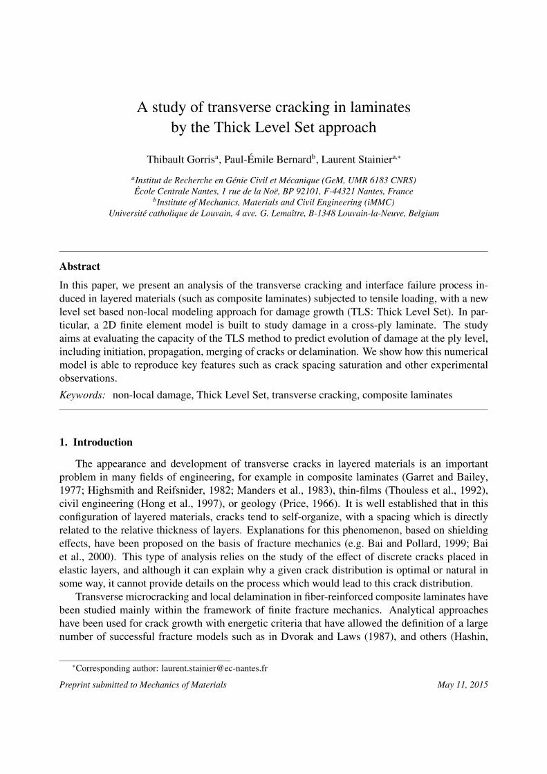
Note that the initiation criterion for new cracks is purely local. Once the local energy releaserate Y reaches a value above the local critical value Yc, a small damaged zone is introduced aroundthe critical point: for example, a level set corresponding to a circular curve Γ of radius r0 suchthat: h < r0 < lc (figure 4). Thus, this is not properly speaking a crack, but a small damaged zone,which can later develop as a fully formed crack, such evolution being controlled by a non-localcriterion. Note also that damage initiation occurs in a range where the local constitutive behavior ismathematically well-posed (i.e. hardening stress-strain relation). Later stages are treated throughthe non-local TLS model, avoiding problems of pathological mesh dependence.

Some level of mesh adaption is required as damaged zones develop, in order to maintain asufficiently accurate geometrical description of the level set (in particular in regions of strong

6

Algorithm 1 Incremental computation of crack initiation and propagation1: initial elastic computation2: search for material point with maximal ratio Y/Yc

3: set load factor µ such that Ymax = Yc and insert first crack4: repeat5: compute Y6: search for location on Γ0 with maximal ratio Y/Yc

7: compute associated load factor µ2n = Yc/Ymax

8: compute load factor increment:

h = amax = k((µn + ∆µ)2 Ymax

Yc− 1

)such that maximal damage front advance is of the order of mesh size

9: move damage front:

a = k⟨(µn + ∆µ)2 Y

Yc− 1

⟩+

10: elastic computation (frozen damage)11: search for material point with maximal ratio Y/Yc

12: insert new crack if Y/Yc ≥ 1 (outside of existing damaged zone)13: until µ ≥ µfinal

curvature, as in a crack tip), as well as for numerical integration purposes. This mesh adaption isperformed by a recursive subdivision algorithm of quadtree type.

3. Model laminate

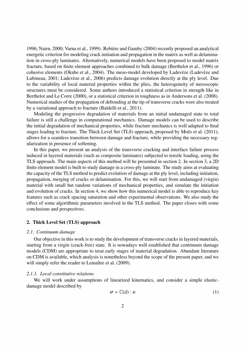
3.1. Geometry and boundary conditionsIn the following, we will consider a composite laminate of type [0m, 90n]s corresponding to

the stacking of unidirectional fiber reinforced plies at orthogonal directions, subject to uniaxialtension. Relative thicknesses of each layer are determined by the number m and n of unit pliesintroduced in the stacking sequence. In the configuration illustrated in figure 5, the fibers in the topand bottom layers are aligned with the tensile axis, and these layers will thus be considered as elas-tic, while fibers in the middle layer are orthogonal to the tensile direction, offering little resistance,and damage will develop in that region. Planar symmetries have been taken into consideration forthe numerical model. Note that the amplitude of the applied tensile force is controlled by a loadfactor, itself computed by the algorithm 1.

3.2. Material propertiesThe top and bottom layers are thus considered as purely elastic (no damage). Rigorously, an

orthotropic elastic stiffness tensor should be used, with different elastic properties in the direc-tion of fibers (ex) and in the transverse direction (ey). Nonetheless, considering that longitudinal

7

Figure 4: Initiation of a new damage zone

Figure 5: Geometry of model laminate

stresses will be dominant over transverse stresses, we will use an isotropic elasticity model withYoung modulus E f and Poisson ratio ν. For the central layer, the material can be considered asisotropic (transverse isotropy) with Young modulus Ec < E f and Poisson ratio ν.

Damage (and cracks) can develop in the central layer, corresponding to matrix failure and/orfiber/matrix debonding. Despite the complexity of micro-mechanisms at work, we will use asimple scalar damage model. We will consider a damage evolution law allowing a progressivetransition from undamaged (d = 0) to totally damaged (d = 1) states, as described by the followingrelation (Ladevèze and Le Dantec, 1992):

d(t) = max0≤τ≤t

⟨ √Y(τ) −

√Y0

√Yu −

√Y0

⟩+

(20)

which can be reformulated through the dissipation pseudo-potential given by:

ψ∗(d; d) =

Yc(d) d if d ≥ 0+∞ otherwise

with Yc(d) =[ √

Y0 + d (√

Yu −√

Y0)]2

(21)

where Y0 is the (initial) critical energy release rate and Yu the ultimate energy release rate (i.e. atcomplete failure).

In order to account for heterogeneities in the material, we introduced a small variability forthe critical energy release rate Y0 in the central layer. This heterogeneity is due to variationsin the density and/or orientation of fibers, as well as other defects, resulting in zones of weaker

8

and higher strength. This variability affects both initiation and propagation of the cracks in thelayer. Various distribution are used in the literature, the use of a particular distribution dependingon the composite and on the physical process considered. Here, following Berthelot and Le Corre(2000), we chose a pseudo-normal distribution (i.e. a normal distribution, but defined on a boundeddomain), but applied on the critical energy release rate (instead of the critical stress in the originalpaper), yielding

Y0 = (σN(0, 1) + 1) Y0 (22)

where N(0, 1) is the normal distribution function, σ the standard deviation, and Y0 the averagevalue of critical energy release rate. In the following, unless explicitly indicated otherwise, we willuse a standard deviation of σ = 0.19. In practice, we obtain a discrete distribution, by drawinga value for each element of the mesh, yielding the distribution illustrated on figure 6. Keeping inline with Berthelot and Le Corre (2000), a “tail” with particularly weak values of Yc was added tothe normal distribution to account for micro-cavities which are known to occur in real materials.Berthelot and Le Corre showed that such weak zones were necessary to reproduce more accuratelycrack density evolution curves in their initial stages.

Figure 6: Distribution of the relative critical energy release rate Yc/Yc over elements of the central layer

The average critical energy release rate Y0 is itself computed from the fracture energy Gc byconsidering the following relation:

Gc = Yc lc ⇐⇒ Y0 =Gc

lc(23)

where Gc is the average fracture energy.9

4. Results

4.1. Influence of algorithmic parametersIn order to assess the effect of algorithmic parameters introduced by the TLS (i.e. d(φ) and lc),

we consider the case studied by Garret and Bailey (1977): a glass/polyester cross-ply composite,with individual plies of thickness 0.8 mm and mechanical properties listed in table 1. The laminateis subjected to tensile loading in the direction corresponding to the orientation of fibers in the topand bottom layers. Note that our numerical model assumes plane strains. The initial mesh size isof the order of 0.05 mm.

Table 1: Material properties for a glass/polyester composite

E f (GPa) Ec (GPa) ν Y0 (MPa) Yu (MPa)23.0 4.2 0.3 0.057 1.3

Given the heterogeneity of the critical energy release rate Yc, damage will first develop in a welllocalized zone, forming a first crack, followed by others as the applied stress increases. Cracks willappear at a distance from each other (as discussed below), leading to a distribution as illustratedin figure 7. Note that adaptive mesh refinement has led to about 40000 degrees of freedom at thisfinal stage.

Figure 7: Transverse crack propagation in a [0, 90, 0] glass/polyester laminate.

4.1.1. Damage profileBefore looking at predictions of our numerical model, we can study the effect of algorithmic

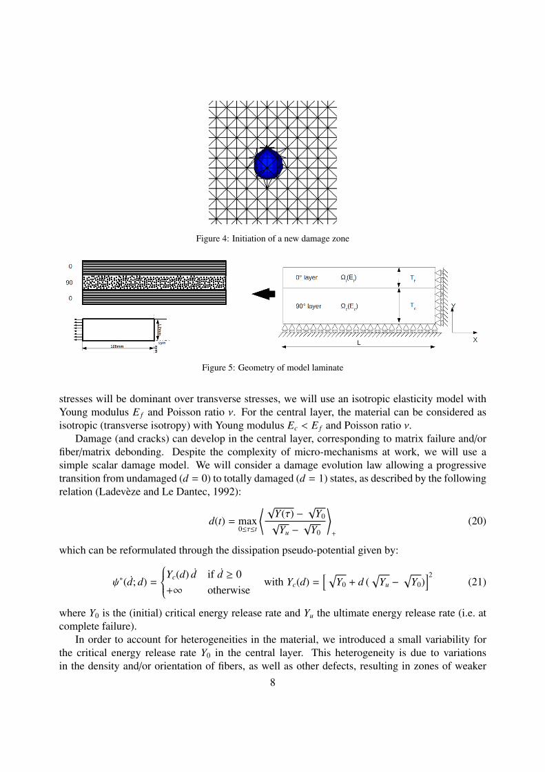
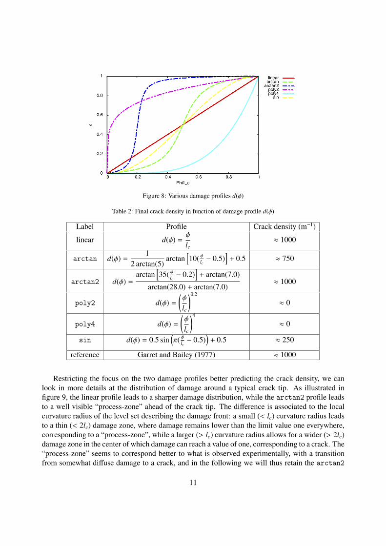
parameters introduced by the TLS approach. First, we will consider a fixed characteristic length,of the order of the diameter of a fiber (lc = 15 µm), and vary the shape of damage function d(φ).Various possibilities are illustrated in figure 8.

One interesting indicator for comparing results is the crack density at the final stage: in com-puting this density, we considered only cracks that have propagated through the middle layer. Thefinal stage can be defined as the stress level for which no more transverse cracks appear, propa-gation of damage occurring instead along the interface between the two layers. Results for thisindicator are given in table 2. These results indicate that the linear and arctan2 profiles pro-vide the best fit with respect to experimental measures. The polynomial profiles lead to very lownumbers: in these cases, new damaged zones seem to be more easily initiated, preventing existingdamaged zones to develop as actual, propagated, cracks.

10

Figure 8: Various damage profiles d(φ)

Table 2: Final crack density in function of damage profile d(φ)

Label Profile Crack density (m−1)

linear d(φ) =φ

lc≈ 1000

arctan d(φ) =1

2 arctan(5)arctan

[10( φlc − 0.5)

]+ 0.5 ≈ 750

arctan2 d(φ) =arctan

[35( φlc − 0.2)

]+ arctan(7.0)

arctan(28.0) + arctan(7.0)≈ 1000

poly2 d(φ) =

(φ

lc

)0.2

≈ 0

poly4 d(φ) =

(φ

lc

)4

≈ 0

sin d(φ) = 0.5 sin(π( φlc − 0.5)

)+ 0.5 ≈ 250

reference Garret and Bailey (1977) ≈ 1000

Restricting the focus on the two damage profiles better predicting the crack density, we canlook in more details at the distribution of damage around a typical crack tip. As illustrated infigure 9, the linear profile leads to a sharper damage distribution, while the arctan2 profile leadsto a well visible “process-zone” ahead of the crack tip. The difference is associated to the localcurvature radius of the level set describing the damage front: a small (< lc) curvature radius leadsto a thin (< 2lc) damage zone, where damage remains lower than the limit value one everywhere,corresponding to a “process-zone”, while a larger (> lc) curvature radius allows for a wider (> 2lc)damage zone in the center of which damage can reach a value of one, corresponding to a crack. The“process-zone” seems to correspond better to what is observed experimentally, with a transitionfrom somewhat diffuse damage to a crack, and in the following we will thus retain the arctan2

11

profile for d(φ).

(a) arctan2 (b) linear

Figure 9: Effect of damage profile on crack tip distribution (both figures are not to scale)

4.1.2. Characteristic lengthConsidering a fixed damage profile, chosen as the arctan2 expression above, we can now

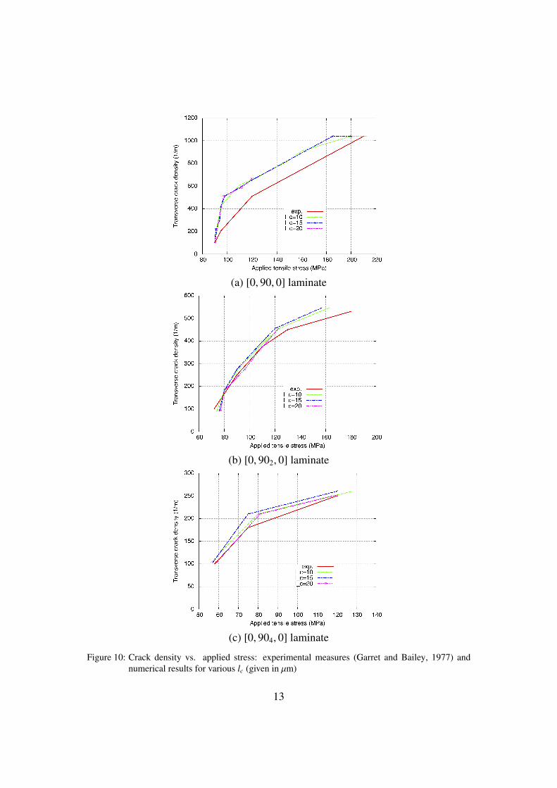
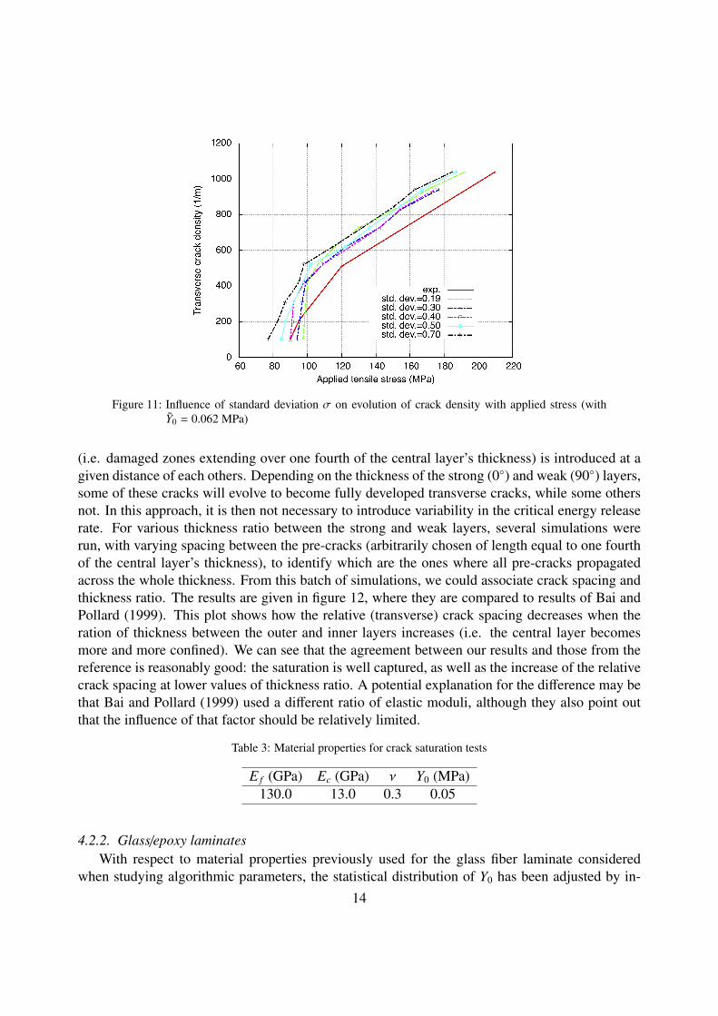
study the effect of the characteristic length lc. We have run the same simulation, with values oflc = 10 µm, lc = 15 µm, and lc = 20 µm. Results can be compared in terms of crack densityevolution in function of applied stress, as illustrated in figure 10, for various stacking sequences(corresponding to different thickness ratios). We can first observe that the parameter lc does notseem to have a significant effect on results. Then, numerical results present a relatively goodagreement with experimental results of Garret and Bailey (1977). The main difference appears forthe case of the [0, 90, 0] laminate, but it must be emphasized that a better fit can actually beobtained by playing with the statistical distribution of Yc. Indeed, increasing the value of standarddeviation up to σ = 0.5 can flatten the crack density curves, as shown in figure 11, and a translationcan be obtained by varying the average value Y0.

4.2. Comparison with experimental data4.2.1. Crack saturation

In multi-layered materials, with layers of different mechanical properties subjected to tensilestress in the longitudinal direction, transverse cracks will appear, parallel to each others. Thesecracks appear in the weaker layers, and are confined by neighboring stronger layers. When longi-tudinal stress/strain increase, the number of cracks increases as well, with new cracks nucleatingbetween existing ones, up to a certain threshold, beyond which no more cracks appear. This satu-ration state is characterized by the distance between cracks. It has been experimentally observed(Garret and Bailey, 1977; Parvizi et al., 1978; Wu and Pollard, 1995) that this distance is relatedto the relative thickness of the weak layer with respect to the strong layer.

In the following, we will verify that our numerical model is able to reproduce this kind ofbehavior. For this purpose, we consider a laminate with material properties listed in table 3. Withinthis preliminary study, we will adopt a strategy slightly different from what was exposed before, inorder to accelerate numerical computations (several successive computations had to be run), andto have a more precise control on crack development. Thus, a number of transverse “pre-cracks”

12

(a) [0, 90, 0] laminate

(b) [0, 902, 0] laminate

(c) [0, 904, 0] laminate

Figure 10: Crack density vs. applied stress: experimental measures (Garret and Bailey, 1977) andnumerical results for various lc (given in µm)

13

Figure 11: Influence of standard deviation σ on evolution of crack density with applied stress (withY0 = 0.062 MPa)

(i.e. damaged zones extending over one fourth of the central layer’s thickness) is introduced at agiven distance of each others. Depending on the thickness of the strong (0) and weak (90) layers,some of these cracks will evolve to become fully developed transverse cracks, while some othersnot. In this approach, it is then not necessary to introduce variability in the critical energy releaserate. For various thickness ratio between the strong and weak layers, several simulations wererun, with varying spacing between the pre-cracks (arbitrarily chosen of length equal to one fourthof the central layer’s thickness), to identify which are the ones where all pre-cracks propagatedacross the whole thickness. From this batch of simulations, we could associate crack spacing andthickness ratio. The results are given in figure 12, where they are compared to results of Bai andPollard (1999). This plot shows how the relative (transverse) crack spacing decreases when theration of thickness between the outer and inner layers increases (i.e. the central layer becomesmore and more confined). We can see that the agreement between our results and those from thereference is reasonably good: the saturation is well captured, as well as the increase of the relativecrack spacing at lower values of thickness ratio. A potential explanation for the difference may bethat Bai and Pollard (1999) used a different ratio of elastic moduli, although they also point outthat the influence of that factor should be relatively limited.

Table 3: Material properties for crack saturation tests

E f (GPa) Ec (GPa) ν Y0 (MPa)130.0 13.0 0.3 0.05

4.2.2. Glass/epoxy laminatesWith respect to material properties previously used for the glass fiber laminate considered

when studying algorithmic parameters, the statistical distribution of Y0 has been adjusted by in-14

Figure 12: Crack saturation effect: comparison with results from Bai and Pollard (1999) (S is the crackspacing, T f and Tc are outer and inner layers’ thickness as defined in fig. 5)

creasing standard deviation σ and average critical energy release rate Y0 to better fit experimentalcrack density curves: looking at figure 11, increasing the value of Y0 allows to shift the curvecorresponding to σ = 0.7 on top of the experimental curve. Note that the value of Yu is basicallylinked to the ultimate strength of the epoxy matrix. The resulting set of data is listed in table 4.

Table 4: Material properties for a glass/epoxy composite

E f (GPa) Ec (GPa) ν Y0 (MPa) σ Yu (MPa)23.0 4.2 0.3 0.08 0.7 1.3

Results obtained from simulations performed with this adjusted set of parameters are shownin figure 13. We can observe the appearance of successive transverse cracks in the weaker cen-tral layer, as the average longitudinal strain increases. New cracks typically initiate at the core ofthe laminate and propagate until they reach the interface between the 90 and 0 layers. One canclearly see on this figure that, as new cracks appear, they tend to respect a spacing equivalent tothe (weak) layer’s thickness (remember that the simulation takes advantage of the transverse sym-metry), which will ultimately lead to saturation (not reached in the numerical simulation presentedhere) as previously discussed.

Figure 14 plots the evolution of transverse crack density as a function of applied longitudinalstress, for various stacking sequences (of type [0, 90n, 0

]) corresponding to a variable thicknessratio between strong and weak layers. These curves are compared with results from Garret andBailey (1977), and exhibit an excellent agreement with this reference.

4.2.3. Carbon fiber reinforced laminatesWe have also considered a the case of carbon fiber reinforced laminates, with an epoxy matrix.

This configuration presents a stronger elastic stiffness ratio between longitudinal (0) and trans-verse (90) directions, as can be seen in table 5. Reference results for this type of laminates are

15

εxx=0.4% (σxx=79 MPa)

εxx=0.41% (σxx=80 MPa)

εxx=0.45% (σxx=85 MPa)

εxx=0.49% (σxx=90 MPa)

εxx=1% (σxx=175 MPa)

εxx=1.2% (σxx=210 MPa)

Figure 13: [0, 90, 0] glass/epoxy laminate: transverse cracks evolution as a function of longitudinalstrain. Average tensile stress has also be indicated for reference. Color map corresponds tostrains.

available in the experimental work of Wang (1984), for example. Here again, parameters describ-ing the statistical distribution of the critical energy release rate have been chosen so as to adjustthe crack density evolution curves: in particular the choice of Y0 allows to set the tensile stress atwhich transverse cracks start to develop significantly.

Table 5: Material properties for a carbon/epoxy composite

E f (GPa) Ec (GPa) ν Y0 (MPa) σ Yu (MPa)76.0 11.7 0.29 0.98 0.7 1.3

Figure 15 shows the evolution of transverse cracks with increasing longitudinal strain, as pre-dicted by the numerical simulations. Again, the transverse cracks are well seen to appear at a

16

Figure 14: Glass/epoxy laminates: crack density evolution with longitudinal stress and comparison withexperimental data from Garret and Bailey (1977)

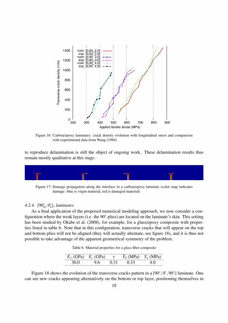
regular distance from each other, as expected. The evolution of transverse crack density withlongitudinal stress is shown on figure 16, for various relative thickness of the laminate layers.Numerical results show a good agreement with experimental measures from Wang (1984).

0.65%

0.75%

1.05%

1.4%

Figure 15: [0, 902, 0] carbon/epoxy laminate: transverse cracks evolution as a function of longitudinal

strain. Color map corresponds to strains, the ruler corresponds to longitudinal coordinate.

Note that in this example, before full saturation of transverse cracks (i.e. for an average lon-gitudinal strain of about 1.4%, as illustrated in fig. 15), damage propagates along the interfacebetween layers, in what resembles a delamination process (see figure 17). This behavior, not ob-served in the previous example, can probably be related to the stronger contrast between the elasticmoduli of the strong and weak layers. Note however that the actual capacity of the TLS approach

17

Figure 16: Carbon/epoxy laminates: crack density evolution with longitudinal stress and comparisonwith experimental data from Wang (1984)

to reproduce delamination is still the object of ongoing work. These delamination results thusremain mostly qualitative at this stage.

Figure 17: Damage propagation along the interface in a carbon/epoxy laminate (color map indicatesdamage: blue is virgin material, red is damaged material)

4.2.4. [90m, 0n]s laminates

As a final application of the proposed numerical modeling approach, we now consider a con-figuration where the weak layers (i.e. the 90 plies) are located on the laminate’s skin. This settinghas been studied by Okabe et al. (2008), for example, for a glass/epoxy composite with proper-ties listed in table 6. Note that in this configuration, transverse cracks that will appear on the topand bottom plies will not be aligned (they will actually alternate, see figure 18), and it is thus notpossible to take advantage of the apparent geometrical symmetry of the problem.

Table 6: Material properties for a glass fiber composite

E f (GPa) Ec (GPa) ν Y0 (MPa) Yu (MPa)30.0 9.6 0.31 0.33 4.0

Figure 18 shows the evolution of the transverse cracks pattern in a [90, 0, 90] laminate. Onecan see new cracks appearing alternatively on the bottom or top layer, positioning themselves in

18

a nonaligned fashion, as expected. The spacing at crack saturation depends, here as well, on therelative thickness of each kind of layer, as it is well visible on figure 18.

0.75%

0.90%

1.20%

1.70%

Figure 18: [90, 0, 90] glass/epoxy laminate: transverse crack evolution as a function of average lon-gitudinal strain (the ruler corresponds to longitudinal coordinate)

[90, 0, 90]

[902, 0, 902]

[903, 0, 903]

Figure 19: Final transverse crack distribution in glass/epoxy laminates with different stacking sequences(the ruler corresponds to longitudinal coordinate)

19

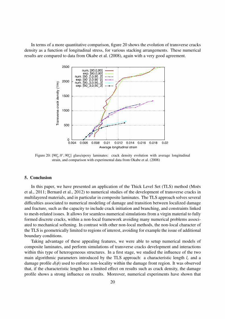
In terms of a more quantitative comparison, figure 20 shows the evolution of transverse cracksdensity as a function of longitudinal stress, for various stacking arrangements. These numericalresults are compared to data from Okabe et al. (2008), again with a very good agreement.

Figure 20: [90n, 0, 90n] glass/epoxy laminates: crack density evolution with average longitudinal

strain, and comparison with experimental data from Okabe et al. (2008)

5. Conclusion

In this paper, we have presented an application of the Thick Level Set (TLS) method (Moëset al., 2011; Bernard et al., 2012) to numerical studies of the development of transverse cracks inmultilayered materials, and in particular in composite laminates. The TLS approach solves severaldifficulties associated to numerical modeling of damage and transition between localized damageand fracture, such as the capacity to include crack initiation and branching, and constraints linkedto mesh-related issues. It allows for seamless numerical simulations from a virgin material to fullyformed discrete cracks, within a non-local framework avoiding many numerical problems associ-ated to mechanical softening. In contrast with other non-local methods, the non-local character ofthe TLS is geometrically limited to regions of interest, avoiding for example the issue of additionalboundary conditions.

Taking advantage of these appealing features, we were able to setup numerical models ofcomposite laminates, and perform simulations of transverse cracks development and interactionswithin this type of heterogeneous structures. In a first stage, we studied the influence of the twomain algorithmic parameters introduced by the TLS approach: a characteristic length lc and adamage profile d(φ) used to enforce non-locality within the damage front region. It was observedthat, if the characteristic length has a limited effect on results such as crack density, the damageprofile shows a strong influence on results. Moreover, numerical experiments have shown that

20

two specific damage profiles (namely a linear expression and an expression in arctan) led tothe most physical results for this specific problem of multilayered materials. In addition, thearctan2 profile led to the appearance of a process zone ahead of the crack tip, in agreementwith many experimental observations in organic matrix composites, and was thus used exclusivelyin the remaining numerical simulations. Ongoing work is aiming at a better and more systematicunderstanding of how the damage profile influences the development of damaged zones and cracks,beyond the conclusions obtained from this particular study.

With these optimized algorithmic parameters, it was shown that the TLS numerical modelwas able to reproduce crack interaction phenomena such as crack saturation in layered materials,showing good agreement with results from the literature, obtained from experimental measures orother computational methods. Several simulations were also performed to study transverse cracksdevelopment within different types of composite laminates ([0, 90n, 0

] and [90n, 0, 90n] stack-

ing sequences), demonstrating both qualitative agreement (e.g. crack placement) and quantitativeagreement (crack densities) with available data from the literature.

Simulations presented in this paper required between 4 hours (for the simpler ones, with pre-existing cracks), up to about 48 hours (for the simulations starting with a virgin material andfinishing with a fully crack-saturated weak layer), on a standard single processor desktop com-puter. Note that there is a lot of room left for optimization of the mathematical solvers, and of thecode itself, and that these computation times have already significantly decreased since the firstsimulations were run.

These results tend to show that the TLS could constitute an interesting approach to studyfracture scenarios and crack patterns in heterogeneous materials such as composites. In some ofthe simulations shown above, one can observe propagation along interfaces once transverse crackssaturation has been reached. As noted before, this qualitatively looks like the early stages of adelamination process. Yet, the proper way to model interfaces between materials (either with ajump of properties or with a smoother gradient), both from the numerical and the physical pointsof view remains an open issue, currently under investigation.

Finally, it is well established that free boundaries effects are absolutely critical in failureprocesses for composite laminates. A reliable numerical analysis of fracture scenarios in lami-nates thus requires to account for three-dimensional models, and the bi-dimensional models usedhere are limited to describe generic effects, such as crack saturation. Implementation of a three-dimensional version of the TLS algorithms has recently been completed, and future work willfocus on such simulations of complex failure scenarios in composites and other heterogeneousmaterials.

Acknowledgements

The authors would like to thank Nicolas Moës (for the many discussions) and Kevin Moreau(for sharing his graphical skills).

References

Andersons, J., Joffe, R., Sparnins, E., 2008. Statistical model of the transverse ply cracking in cross-ply laminates bystrength and fracture toughness based failure criteria. Engineering Fracture Mechanics 75 (9), 2651–2665.

21

Bai, T., Pollard, D. D., 1999. Spacing of fractures in a multilayer at fracture saturation. International Journal ofFracture 100, L23–L28.

Bai, T., Pollard, D. D., Gao, H., 2000. Explanation for fracture spacing in layered materials. Nature 403, 753–756.Baldelli, A. A. L., Bourdin, B., Marigo, J.-J., Maurini, C., 2011. Étude de la multifissuration et délamination par

l’approche variationnelle à la mécanique de la fracture. In: 10e colloque national en calcul des structures. Giens,France, p. 8 p.URL https://hal.archives-ouvertes.fr/hal-00592809

Bernard, P.-E., Moës, N., Chevaugeon, N., 2012. Damage growth modeling using the thick level set (tls) approach:efficient and accurate discretization for quasi-static loadings. Computer Methods in Applied Mechanics and Engi-neering 233-236, 11–27.

Berthelot, J.-M., Le Corre, J.-F., 2000. Statistical analysis of the progression of transverse cracking and delaminationin cross-ply laminates. Composites Science and Technology 60 (14), 2659–2669.

Berthelot, J.-M., Leblond, P., Mahi, A. E., Le Corre, J.-F., 1996. Transverse cracking of cross-ply laminates: Part 1.analysis. Composites Part A: Applied Science and Manufacturing 27 (10), 989–1001.

Dvorak, G. L., Laws, N., 1987. Analysis of progressive matrix cracking in composites laminates. Journal of Compos-ites Materials 21 (4), 309–329.

Garret, K., Bailey, J., 1977. Multiple transverse cracking in 90 cross-ply laminates of a glass fibre-reinforcedpolyester. Journal of Materials Science 12, 157–168.

Germain, P., Nguyen, Q. S., Suquet, P., 1983. Continuum thermodynamics. Journal of Applied Mechanics 50, 1010–1020.

Halphen, B., Nguyen, Q. S., 1975. Sur les matériaux standard généralisés. J. Mécanique 14 (1), 39–63.Hashin, Z., 1996. Finite thermoelastic fracture criterion with application to laminate cracking analysis. Journal of the

Mechanics and Physics of Solids 44 (7), 1129–1145.Highsmith, A. L., Reifsnider, K. L., 1982. Stiffness-reduction mechanisms in composite laminates. In: Reifsnider,

K. L. (Ed.), Damage in Composite Materials. ASTM STP 775, pp. 103–177.Hong, A., Li, Y., Bazant, P., 1997. Theory of crack spacing in concrete pavements. Journal of Engineering Mechanics

123, 267–275.Ladevèze, P., Le Dantec, E., 1992. Damage modelling of the elementary ply for laminated composites. Composites

Science and Technology 43 (3), 257–267.Ladevèze, P., Lubineau, G., 2001. On a damage mesomodel for laminates: micro-meso relationships, possibilities and

limits. Composites Science and Technology 61 (15), 2149–2158.Ladevèze, P., Lubineau, G., Marsal, D., 2006. Towards a bridge between the micro- and mesomechanics of delamina-

tion for laminated composites. Composites Science and Technology 66 (6), 698–712.Lemaître, J., Chaboche, J. L., Benallal, A., Desmorat, R., 2009. Mécanique des matériaux solides, 3rd Edition. Dunod.Manders, P. W., Chou, T. W., Jones, F. R., Rock, J. W., 1983. Statistical analysis of multiple fracture in 0/90/0

glass fibre/epoxy resin laminates. Journal of Materials Science 18 (10), 2876–2889.Moës, N., Stolz, C., Bernard, P., Chevaugeon, N., 2011. A level set based model for damage growth: The thick level

set approach. International Journal for Numerical Methods in Engineering 86 (3), 358–380.Nairn, J. A., 2000. Exact and variational theorems for fracture mechanics of composites with residual stresses,

traction-loaded cracks, and imperfect interfaces. International Journal of Fracture 105 (3), 243–271.Okabe, T., Nishikawa, M., Takeda, N., 2008. Numerical modeling of progressive damage in fiber reinforced plastic

cross-ply laminates. Composites Science and Technology 68 (10-11), 2282–2289.Okabe, T., Sekine, H., Noda, J., Nishikawa, M., Takeda, N., 2004. Characterization of tensile damage and strength in

GFRP cross-ply laminates. Materials Science and Engineering A 383 (2), 381–389.Parvizi, A., Garrett, K., Bailey, J., 1978. Constrained cracking in glass fiber-reinforced epoxy cross-ply laminates.

Journal of Materials Science 13 (3), 195–201.Peerlings, R., de Borst, R., Brekelmans, W., de Vree, J., 1996. Gradient enhanced damage for quasi-brittle materials.

International Journal for Numerical Methods in Engineering 39 (19), 3391–3403.Pijaudier-Cabot, G., Bažant, Z., 1987. Nonlocal damage theory. Journal of Engineering Mechanics 113 (10), 1512–

1533.Price, N. J., 1966. Fault and Joint Development in Brittle and Semi-Brittle Rocks. Oxford, Pergamon Press.

22

Rebière, J.-L., Gamby, D., 2004. A criterion for modelling initiation and propagation of matrix cracking and delami-nation in cross-ply laminates. Composites Science and Technology 64 (13-14), 2239–2250.

Thouless, M. D., Olsson, E., A., G., 1992. Cracking of brittle films on elastic substrates. Acta Metallurgica Materialia40, 1287–1292.

Varna, J., Joffe, R., Akshantala, N. V., Talreja, R., 1999. Damage in composite laminates with off-axis plies. Compos-ites Science and Technology 59 (14), 2139–2147.

Wang, A. S. D., 1984. Fracture mechanics of sublaminate cracks in composite materials. Journal of Composites,Technology and Research 6 (2), 45–62.

Wu, H., Pollard, D. D., 1995. An experimental study of the relationship between joint spacing and layer thickness.Journal of Structural Geology 17 (6), 887–905.

23