Southeast Asian Studies, Vol. 37, No.3, December 1999 A Study on Estimation of Cassava Area and Production Using Remote Sensing and Geographic Information Systems in the Northeast Region of Thailand Apisit EIUMNOH* and Rajendra P. SHRESTHA* Abstract A study on cassava plantation area and production was conducted in the northeast region of Thailand using an integrated Satellite Remote Sensing (SRS) and Geographic Informa- tion Systems (GIS). Although, SRS and GIS are considered as the efficient tools for resource inventorying and monitoring, little work has been done in Thailand with regards to the large area crop monitoring and production estimation. The objective of the study was to explore the use of NOAA-AVHRR data for mapping cassava plantation areas. GIS was employed to create geographical database, such as soils, topography, land use and also for improving the results of image classification. The study conducted for the two crop seasons of 1995 and 1996 indicated that the NOAA-A VHRR data can be used to map the cassava plantation areas at the regional scale in Thailand. The results of the study were compared with existing cassava statistics produced from the Thai Tapioca Development Institute (TTDI) and the Office of Agricultural Economics (GAE), Thailand. The estimated cassava plantation areas from the study were underestimated by - 9.7 and - 16.4 percent to that of TTDI and OAE, respectively for 1995 and overestimated by 4.0 percent but underestimated by - 14.4 percent, respectively for the year 1996. I Introduction I-1 Cassava Plantation in Thailand Cassava called as Tapioca (Manihot esculenta Crantz) is one of the major export crops of Thailand. There has been tremendous increase in cassava plantation area in the country in the last three decades, from 71,520 ha in 1960 to 1,228,111 ha in 1996 [OAE 1974; 1996, respectively]. Van der Eng [1998J mentioned that in the 1960s, Thailand took over Indonesian position as Asia's main cassava exporter. The crop gained considerable popularity among the Thai farmers because of the two main reasons: increased demand of cassava roots in the foreign market though the farm-gate price has been fluctuated over time, and the crop's excellent adaptability in the adverse climatic and biophysical condition. The crop performs well on poor upland soils, has high tolerance to drought, diseases and insect pests, and more importantly its flexible planting and harvesting times * School of Environment, Resources and Development of the Asian Institute of Technology, P. O. Box 4, Klongluang 12120, Thiland 417
Transcript
Southeast Asian Studies, Vol. 37, No.3, December 1999
A Study on Estimation of Cassava Area and ProductionUsing Remote Sensing and Geographic Information
Systems in the Northeast Region of Thailand
Apisit EIUMNOH* and Rajendra P. SHRESTHA*
Abstract
A study on cassava plantation area and production was conducted in the northeast regionof Thailand using an integrated Satellite Remote Sensing (SRS) and Geographic Information Systems (GIS). Although, SRS and GIS are considered as the efficient tools forresource inventorying and monitoring, little work has been done in Thailand with regardsto the large area crop monitoring and production estimation. The objective of the studywas to explore the use of NOAA-AVHRR data for mapping cassava plantation areas. GISwas employed to create geographical database, such as soils, topography, land use and alsofor improving the results of image classification. The study conducted for the two cropseasons of 1995 and 1996 indicated that the NOAA-AVHRR data can be used to map thecassava plantation areas at the regional scale in Thailand. The results of the study werecompared with existing cassava statistics produced from the Thai Tapioca DevelopmentInstitute (TTDI) and the Office of Agricultural Economics (GAE), Thailand. The estimatedcassava plantation areas from the study were underestimated by - 9.7 and - 16.4 percentto that of TTDI and OAE, respectively for 1995 and overestimated by 4.0 percent butunderestimated by - 14.4 percent, respectively for the year 1996.
I Introduction
I - 1 Cassava Plantation in Thailand
Cassava called as Tapioca (Manihot esculenta Crantz) is one of the major export crops of
Thailand. There has been tremendous increase in cassava plantation area in the country
in the last three decades, from 71,520 ha in 1960 to 1,228,111 ha in 1996 [OAE 1974; 1996,
respectively]. Van der Eng [1998J mentioned that in the 1960s, Thailand took over
Indonesian position as Asia's main cassava exporter. The crop gained considerable
popularity among the Thai farmers because of the two main reasons: increased demand
of cassava roots in the foreign market though the farm-gate price has been fluctuated
over time, and the crop's excellent adaptability in the adverse climatic and biophysical
condition. The crop performs well on poor upland soils, has high tolerance to drought,
diseases and insect pests, and more importantly its flexible planting and harvesting times
* School of Environment, Resources and Development of the Asian Institute of Technology,P. O. Box 4, Klongluang 12120, Thiland
417
Table 1 Plantation Area, Yield and Production of Cassava in Northeast Thailand
Sources: [OAE 1979; 1982; 1985; 1993; 1996; 1998JNote: The production is estimated based on the yield and harvested area. The
proportion of actual harvested area ranged from 91 percent in 1985 to 97percent in 1996 of the total planted area.
ensure the farm return. This means that the crop can be left out in the field without
taking harvest until the farmer is satisfied with the price for his crop. Next crop of
cassava can be planted right after the harvesting.
Geographically, Thailand can be divided into four regions: the North, Northeast,
Central and South region. The northeast region is the largest cassava grower among the
four regions. The region constitutes about 62 percent of the total cassava plantation area
and about 70 percent of the total cassava production in the country [OAE 1996J. The
region has experienced a tremendous increase in cassava plantation area from 1975 to
1990 with an annual average of 46,525 hat Since 1990, the total cassava plantation area has
been decreasing slowly with an average rate of 27,470 ha per year (Table 1).
Crop area monitoring is important from the agricultural planning point of view. In
Thailand, the annual agricultural statistical data on crop acreage, production and yield
are prepared by applying statistical projection techniques on the field information
collected through sampled interviews. The process of data compilation and report
production involves quite long time, at least six months. Early availability of these data
can be valuable for several purposes, one of these being the agricultural trade for export
and estimating the revenue.
I - 2 Satellite Remote Sensing and Geographic Information SystemsSatellite Remote Sensing (SRS) has been applied in several instances of natural resources
monitoring, such as wetland vegetation monitoring [Yasuoka et at. 1995J, deforestation
monitoring [Hirano et at. 1995J, drought monitoring [Lozano-Garcia et al. 1995J, land use
change [Pande and Saha 1994J, including agricultural monitoring, such as corn, soybeans,
sugarbeets area monitoring [Ehrlich et at. 1994J, irrigated crops monitoring [Manavalan etat. 1995J using both the optical and microwave data.
418
A. EWMNoH and R. P. SHRESTHA : Estimation of Cassava Area and Production
Uses of satellite data from Advanced Very High Resolution Radiometer (AVHRR)
sensor of National Oceanic and Atmospheric Administration (NOAA) satellite for crop
area estimation and yield modeling have also been demonstrated by many researchers,
such as Groten [1993J, and Potdar [1993]. This data has also been used for crop area and
yield estimates in different parts of the world, such as in the United States [Hayes et at.
1991J, Africa [Maselli et at. 1992J, Canada [Hayes and Decker 1996; Korporal 1993J, and
Europe [Benedetti and Rossini 1993].
The proportion of vegetative biomass in the area being sensed or captured in the
satellite data is important for later interpretation. In crop monitoring, the stage of crop
growth is thus important in terms of significant spectral responses of the features in the
data. For example, in case of cassava there is higher spectral response from the cassava
alone during its peak vegetative growth and lesser response during early period due to
less crown cover (Fig. 1).
Remote sensing technique, which has been used for real-time monitoring and even
for an early production assessment in many parts of the world, has not been yet
operationalize in Thailand. Hence, the main objective of this study was to explore the
potential of remote sensing technique to classify the cassava area and monitor the
production using NOAA-AVHRR data in the northeast Thailand.
High
0-1 1 - 2 2-3
DecemberMonth----------------------1.... November
Fig. 1 Stages of Cassava Growth and Spectral Responses in the Satellite Data
419
IT Methodology
IT - 1 The Study A rea
The northeast region, located between 14°06 '-18°35' N latitude and 101°06 '-105°21 ' E
longitude, is the largest region of Thailand with its 19 provinces covering over 170,000
km 2 (Fig. 2).
The climate of the area can be characterized as the tropical wet-dry climate with
extreme low and high temperatures of 6.6° to 41.6° Celsius (C), respectively with the
annual mean of 26.6°C (1991-1995). There is high degree of variation in annual rainfall
amount in different parts within the region. In general, the southern part of the region
is drier than the northern part. During 1991-1995, the average annual rainfall amount and
annual rainyday were 1,041 mm and 105 days, respectively in Nakhon Ratchasima, where
as they were 2,240 mm and 137 days in Nakhon Phanom province [OAE 1996].
The topography is gently undulating all over the region except the plain areas
between the Chi and Mun rivers and to the south of the Mun river. The soils are mostly
light texture of sandy Paleaquult in the depression and Paleustults in the upland with low
moisture holding capacity and fertility [Eiumnoh and Shrestha 1997J. However, the
region is inhabited by over one-third of country's population, the income per farm family
Northeast region of Thailand
'"80400' N~
ii
I
I 100 0 100 Kilometers
/ ~ ~
i ~.,
l~._~_~
----~--~-----~~------------------~~--
Fig. 2 Location of the Study Area
420
A. EIUMNOH and R. P. SHRESTHA: Estimation of Cassava Area and Production
of 1,247 US$ in the northeast region was almost half of the country's average farm income
of 2,473 US$ in 1995/96 [OAE 1998J. The unstable agricultural production is one of the
major reasons for low farm income. The critical constraints that influence agriculture in
the region are soil, topography, water supply and erratic rainfall.
n- 2 Data Types
The basic data sources were NOAA-AVHRR data acquired by NOAA-14 satellite, existing
topographic maps (scale 1: 250,000; The Royal Thai Survey Department, Bangkok, 1984),
land use map of 1993 (scale 1: 250,000; OAE, Bangkok), soil map (scale 1: 500,000; Soil
Survey Division, Bangkok, 1982), and the published agricultural statistics. The field
surveys in all the provinces of the region were conducted to carry out ground truthing
for cassava cultivation and verify the land use map.
The baseline spatial database on province boundaries, land uses and soil types were
prepared by digitizing the required information from the above-mentioned base maps
using PC Arc/Info software.
The AVHRR senses in five wavebands ranging in the visible (band 1,0.58 - 0.68 ,urn),
the near infrared (band 2, 0.725 - 1.10 ,urn), and thermal infrared (band 3, 3.55 - 3.93 ,urn;
band 4, 10.5 - 11.5 ,urn; band 5, 11.5 - 12.5 ,urn) regions of the electromagnetic spectrum at a
nadir pixel resolution of 1.1 km by 1.1 km [Kidwell 1995J. Many of more recent studies
have utilized the Normalized Difference Vegetation Index (NDVI), a ratio of reflectance in
the near infrared and red wavelengths of the spectrum [Robinson 1996]. The AVHRR
data are suitable for macro-assessment and monitoring of land cover status and their
change patterns in near real time basis [Giri and Shrestha 1995]. One of the major
advantages of the data is its synoptic coverage as one scene of AVHRR data can cover the
whole country of Thailand, which otherwise require about 12 full scenes of Landsat
Thematic Mapper (TM) to cover the northeast region of Thailand only. Table 2 reviews
the strengths and weaknesses of AVHRR data.
The study employs an integration of SRS, GIS and other ancillary information from
the field survey and secondary sources. The AVHRR data for two years period (1995 and
Table 2 Strengths and Weaknesses of NOAA-AVHRR Data
Strengths Weaknesses1. Synoptic coverage and hence, low 1. Coarse resolution (1.1 km at nadir)
data volume 2. Preprocessing is time consuming2. High radiometric resolution (lO-bit) 3. Basically a weather monitoring data, hence3. Relatively low cost the methodology in handling AVHRR data for4. High opportunity for real time data land applications is not well developed
due to its daily revisit 4. LAC data has limited capability to record on-5. Twice daily coverage and hence board
high possibilities of having cloud 5. Data acquired in rainy season (crop growingfree data season) has problem of cloud
Source: Modified from Giri and Shrestha [1995J
421
1996) were used in the study. The data selected for the year 1995 was acquired on 25
November 1995, and for 1996 were 24 and 26 December. Unlike the microwave radar data,
which can penetrate the cloud, the optical dataset has the cloud related problem during
the crop growing season in the tropical region, like Thailand. Among the data acquired
during the crop season for the respective years, the selection of data was made based on
the minimum percentage of cloudy pixels in the data.
IT - 3 A VHRR Data Processing
The raw AVHRR data were taken through a number of preprocessing steps before the
analysis was carried out. The calibration procedures, which are adopted for AVHRR data
preprocessing by the National Environmental Satellite Data and Information Service
(NESDIS) were used for this study. The percentage albedo of visible and infrared
channels was calculated and was converted to radiance value. The thermal channels
were also converted to radiance values. The radiance for all channels were calculated
using the channel related linearity and non-linearity calibration coefficients given for
NOAA-14. As there were two date images for the year 1996, a cloud masked composite
image was prepared from 24 and 26 December images.
For the geometric correction of raw images, 60 Ground Control Points (GCPs) were
collected from the topographic map and then the raw images were registered to the
topographic map with the help of those selected GCPs. The Root Mean Square (RMS)
error accepted was less than 1 pixel at the third order of nearest neighbor transforma
tion.
The usual technique of estimating crop area by using remote sensing is the direct
estimate from classified image. The most obvious area estimator from a classified image
is
Zc=~DN pix
where, Zc is the area estimator,,uc is the number of pixels classified into the land use
c, Npix is the total number of pixels, and D is the total area [Gallego et al. 1993J. The image
can be classified by supervised and unsupervised techniques. Supervised technique is a
user control where the whole image is classified based on the user defined training areas,
where as in the unsupervised technique, the pixels are assigned to the certain groups
instead of user defined training areas but the threshold values for separating different
classes. In the supervised technique, homogenous areas are required for selecting as the
training areas. Given the land use pattern of the study area where many types of land use
exists in a one sq. km. area (pixel resolution of NOAA-AVHRR), not enough areas for
training the signatures were possible. Hence, an ISODATA clustering technique was
used to classify the images using original bands, ratio bands and NDVI assigning
altogether 40 classes which were later regrouped based on the Ward's method of hierar-
422
A. EIUMNoH and R. P. SHRESTHA: Estimation of Cassava Area and Production
chical clustering technique. This method calculates means for each variable within each
cluster and squared Euclidean distance to the cluster means for each case [Aldenderfer
and Blashfield 1984J. The final classification map was prepared by merging the clusters
which result in the smallest increase in the overall sum of the squared within cluster
distance.
The result of image classification was evaluated by computing Overall Classification
Accuracy (OCA), i. e. the proportion of correctly classified pixels of the total pixels of the
classified image. Construction of error matrix to express the OCA is the most common
technique [Lillesand and Kiefer 1994]. A sample size of 196 pixels were determined using
the following formula from the binomial probability theory [Fitzpatrick-Lins 1981J.
where, Z = 1.96 as the normal standard deviate for the 95% two-sided confidence
interval, p = 85% as the expected percent accuracy, q = 100 - p, and E = 5 % allowable
error. The sample pixels were randomly selected for each of the classified image to
construct the error matrices and then find out the correctly classified pixels with the help
of available reference information, such as field information and land use map.
II - 4 SRSjGIS Integration
The clustering process of image classification operates on the spectral signature of the
pixel of the image. It means that a pixel is classified into only one class although it
contains more than one land use types. Considering the prevailing land use pattern of the
area, such situation of more than one land use type within a pixel is often likely to occur.
In some instances, it might also be possible that the signatures of cassava resembles with
sparse forest and bushy area, which also introduces error in the classification results by
not being able to distinctly separate them because of the similar signatures of different
classes.
The purpose of integrating the GIS to the classified NOAA-AVHRR images was to
improve the classification results obtained from image data by post-classification sorting.
The topographic information and soil information are strongly correlated in determining
the certain type of land use. For example, cassava is not cultivated in the lowland or soils
having aquic moisture regime. Use of larger scales or resolutions GIS database, as those
in this study, compared to that of NOAA-AVHRR helps to improve the result of image
classification, which is solely based on the spectral signature of the pixel.
The classified images were imported to GIS, where vector layers of land use, soil map
and province boundaries were overlaid. Then, a sequential masking was followed to
eliminate the land uses other than cassava on the basis of soil types and land use types
(Fig. 3). For example, in the first step, all the non-agricultural areas were masked by
using land use map. Thus, all the pixels mis-classified as cassava in the non-agricultural
423
Provincewlsecassava area
Soil map
Provinceboundary map J----------------..I.----.
Land usemap
Vectorizedclassified image
with differentland use classes
Fig. 3 GIS Procedure for Sequential Masking
areas were eliminated. In the second step, all the pixels, mis-classified as cassava in the
lowland area (having aquic regime or paddy soil), were eliminated by overlaying the soil
map. The results were reevaluated by computing OCA following the same procedure
described earlier. Finally, province boundary layer was overlaid to estimate the cassava
plantation area in each province.
ill Results and Discussion
m- 1 Comparison of Existing Agriculture Statistics
The crop acreage and production of cassava have been reported regularly on the annual
basis from the Thai Tapioca Development Institute (TTDI) and Office of Agricultural
Economics (OAE). For the year 1995, the total cassava plantation area in the northeast
region of Thailand was reported to be 748,640 ha by TTDI, where as it was 808,741
according to OAE statistics (Table 3). The differences between the reported statistics
could be probably because of the method of data collection and data projection tech
niques of the individual organization. The technique of data collection is the interview
of sample farmers or key informants by the field workers in both the cases (personal
communication). Since, the organizational setup is different, in most cases it is likely that
the sampled interviews with different interviewee and level of sampling lead to the
generation of different statistics.
Data discrepancies can also be found with other existing information. For example,
we also digitized the land use map of 1993 produced by OAE and calculated the cassava
plantation area in the study area. The GIS derived cassava plantation area was much
higher (1,495,248 ha) than the tabular data. It could be due to various reasons, such as
map accuracy and map scale where the area is overestimated when smaller map units are
masked and thus generalized during the visual classification. This shows the obvious
discrepancies in the existing data generated by not only different organizations but also
424
A. EIUMNOH and R. P. SHRESTHA: Estimation of Cassava Area and Production
Table 3 Cassava Plantation Area in N. E. Thailand from Different Sources
different data format. Such situation exhibits the need of a reliable baseline study
employing a firm technique and efficient too.
ill- 2 Cassava Area Estimation
The overall classification accuracies obtained for the classified images from the digital
image processing technique alone were 74 and 78 percent for the year 1995 and 1996,
respectively.
As discussed earlier, the cassava has prolonged planting and harvesting times. The
prolonged harvesting period means even after the crop is at harvestable stage, can be left
as such in the field for few weeks without taking harvest. It was learnt from the farmers
that the yield loss due to late harvesting is not of much significance. However, the major
harvesting period is from November to January. The next crop is planted right after
harvesting using stem cuttings as planting materials. This implies that there can be
different stages of the crop in terms of its vegetative growth at a particular point of time.
Since AVHRR data is a coarse resolution (1.1 km) data, it is possible that not only
different stages of cassava field can be found in the given resolution but also different
land use types, which popularly can be called as "mixed pixel" condition. Such condition
can be dealt by overlaying the GIS database with the classified images for the post
classification sorting.
425
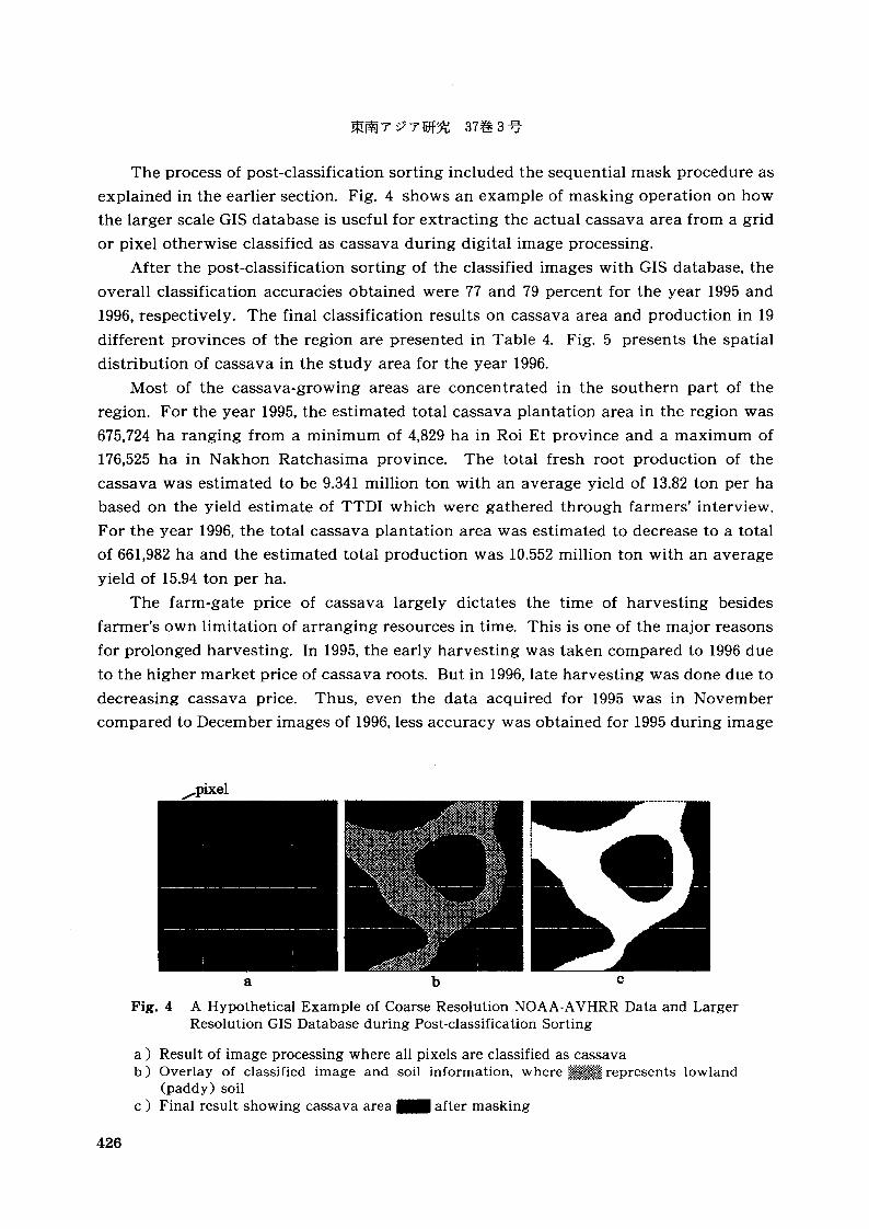
The process of post-classification sorting included the sequential mask procedure as
explained in the earlier section. Fig. 4 shows an example of masking operation on how
the larger scale GIS database is useful for extracting the actual cassava area from a grid
or pixel otherwise classified as cassava during digital image processing.
After the post-classification sorting of the classified images with GIS database, the
overall classification accuracies obtained were 77 and 79 percent for the year 1995 and
1996, respectively. The final classification results on cassava area and production in 19
different provinces of the region are presented in Table 4. Fig. 5 presents the spatial
distribution of cassava in the study area for the year 1996.
Most of the cassava-growing areas are concentrated in the southern part of the
region. For the year 1995, the estimated total cassava plantation area in the region was
675,724 ha ranging from a minimum of 4,829 ha in Roi Et province and a maximum of
176,525 ha in Nakhon Ratchasima province. The total fresh root production of the
cassava was estimated to be 9.341 million ton with an average yield of 13.82 ton per ha
based on the yield estimate of TTDI which were gathered through farmers' interview.
For the year 1996, the total cassava plantation area was estimated to decrease to a total
of 661,982 ha and the estimated total production was 10.552 million ton with an average
yield of 15.94 ton per ha.
The farm-gate price of cassava largely dictates the time of harvesting besides
farmer's own limitation of arranging resources in time. This is one of the major reasons
for prolonged harvesting. In 1995, the early harvesting was taken compared to 1996 due
to the higher market price of cassava roots. But in 1996, late harvesting was done due to
decreasing cassava price. Thus, even the data acquired for 1995 was in November
compared to December images of 1996, less accuracy was obtained for 1995 during image
~ .
I.a b c
Fig. 4 A Hypothetical Example of Coarse Resolution NOAA-AVHRR Data and LargerResolution GIS Database during Post-classification Sorting
a) Result of image processing where all pixels are classified as cassavab) Overlay of classified image and soil information, where ~.:! represents lowland
(paddy) soilc) Final result showing cassava area _ after masking
426
A. EIUMNOH and R. P. SHRESTHA : Estimation of Cassava Area and Production
Table 4 Classified Cassava Plantation Area and Production in N. E. Thailand
1995 1996Province Area Yie1d* Production Area Area Yield* Production Area
Total 675,724 13.82 9,341,205 72,916 661,982 15.94 10,551,797 - 25,166
Notes: * Yield estimates from TTDI** Denotes the difference between TTDI's report and image classified area, e. g. in 1995,
TTDI's reported area was higher by 79,474 ha for Nakhon Ratchasima but was lower by- 13,767 ha for Buri Ram province.
classification due to higher percentage of already harvested cassava fields, and thus
representing the bare field.
N Conclusion and Further Work
The study conducted in the northeast region of Thailand for the two years indicated that
NOAA-AVHRR data can be considered for the operational cassava area monitoring.
However, it was somewhat difficult in deciding to which source be considered as the
baseline data for the evaluation of study results due to the differences in the statistics
produced by different organizations. The comparison between the findings of the study
and the existing statistics from TTDI and OAE showed that the estimated cassava
plantation area from the study was closer to that of TTDI with - 9.7 percent under
estimated for the year 1995 and 4.0 percent overestimated for 1996. In case of OAE
statistics, the estimated cassava areas were underestimated by - 16.4 and - 14.4 percent
for the year 1995 and 1996, respectively.
Nevertheless, remote sensing and geographic information systems techniques are
427
05E
_ cassava area
N
O2E
O2E.....1l....50..._ ..1001llomMlr O5E
Fig. 5 Spatial Distribution of Cassava Area in the Northeast Region of Thailand in 1996
useful tools for the crop area estimation, and certainly efficient over existing techniques
for obtaining quicker and reliable results. Integration of geographic information systems
at the post-classification stage of the image analysis improved the result than remote
sensing technique alone in case of coarser resolution data, like NOAA-A VHRR.
Regarding the data acquisition, use of the single date data gives satisfactory result in
those years of late harvesting. Considering the different harvesting time of the crop, it is
desirable to use the time series data as the single date data do not represent all those
cassava fields which were already harvested before the data acquired. But one of the
problems in using time series data is the cloud cover in the NOAA-AVHRR data during
September-Dctober, which is the best period for data acquisition. For operationalizing
the remote sensing for cassava area monitoring, the cloudfree composite image could be
prepared from the several data acquired during this period (September-October), how
ever it requires more resources towards data purchasing and processing, and which was
beyond the scope of the study. Analysis of such composite image could help to correctly
assess the cassava plantation areas with higher accuracy.
There are also opportunities to deal with the cloud related problem by making use of
microwave remote sensing, which can penetrate the cloud and sense the earth features,
428
A. EIUMNoH and R. P. SHRESTHA: Estimation of Cassava Area and Production
but needs further studies as this technology is still in infant stage in this area of
application.
Acknowledgement
The authors would like to acknowledge the generous support of the Thai Tapioca DevelopmentInstitute, Bangkok for providing the financial support, National Research Council of Thailand forproviding AVHRR data and the Asian Institute of Technology, Bangkok for the research facilities tocarry out the study. Comments of the anonymous referees and the editor on the manuscript arehighly appreciated.
References
Aldenderfer, M. S.; and Blashfield, R K 1984. Cluster Analysis. London: SAGE Publications, Inc.Benedetti, R; and Rossini, P. 1993. On the Use of NDVI Profiles as a Tool for Agricultural Statistics:
The Case Study of Wheat Yield Estimate and Forecast in Emilia Romagna. Remote SensingEnviron 45: 311-326.
Ehrlich, d. Estes]. E.; Scepan,].; and McGwire, K C. 1994. Crop Area Monitoring within an AdvancedAgricultural Information System. Geocarto International 4: 31-41.
Eiumnoh, A.; and Shrestha, R. P. 1997. Integration of Remote Sensing and Geographic InformationSystems for Cassava Monitoring in the Northeast Thailand: Problems Still Exist. In CD ROMProc. of "GER" 97: Geomatics in the Era of RADARSA T 1997, Ottawa, Canada, 25-30 May 1997.
Fitzpatrick-Lins, K 1981. Comparison of Sampling Procedures and Data Analysis for a Land-use andLand-cover Map. Photogrammetric Engineering and Remote Sensing 47 (3): 343-351.
Gallego, F.].; Delince, J.; and Rueda, C. 1993. Crop Area Estimates through Remote Sensing: Stabilityof the Regression Correction. Int. J Remote Sensing 14 (18): 3433-3445.
Giri, C. P.; and Shrestha, S. 1995. Developing Land Cover Classification System for NOAA-AVHRRApplications in Asia. In Proc. of the 16th Asian Conference on Remote Sensing, 20-24 November1995, Nakhon Ratchasima, Thailand.
Groten, S. M. E. 1993. NDVI-Crop Monitoring and Early Yield Assessment of Burkino Fasa. Int. JRemote Sensing 14 (8): 1495-1515.
Hayes, M.].; and Decker, W. L. 1996. Using NOAAHRR Data to Estimate Maize Production in theUnited States Corn Belt. Int.]. Remote Sensing 17 (16): 3189-3200.
Hayes, M. J.; Decker, W.; and Achutuni, V. 1991. Relationships between the NDVI and Crops Yieldsalong a Transect across the Great Plains. In Proc. of the Twentieth Conference on Agricultural andMeteorology, Salt Lake City, UT, 10-13 September. pp. 102-104. Boston: American MeteorologicalSociety.
Hirano, A.; Saito, G.; and Mino, N. 1995. Monitoring Deforestation in Luzon Island, the PhilippinesUsing Satellite Data. In Proc. of the 16th Asian Conference on Remote Sensing, 20-24 November1995. Nakhon Ratchasima, Thailand.
Kidwell, K 1995. NOAA Polar Orbiter Data User's Guide. Washington, D. C.: NOAA/NESDIS.Korporal, K 1993. Early Season Yield Estimates 1993. Agricultural Division, Statistics Canada.
Ottawa, Canada. (unpublished)Lillesand, T. M.; and Kiefer, R W. 1994. Remote Sensing and Image Interpretation. The third edition.
Singapore: John Wiley and Sons.Lozano-Garcia, D. F.; Fernandez, R. N.; Gallo, K P.; and Johannsen, c.]. 1995. Monitoring the 1988
Severe Drought in Indiana, U. S. A. Using AVHRR Data. Int. J Remote Sensing 16 (7): 1327-1340.Manavalan, P.; Kesavasamy, K; and Adiga, S. 1995. Irrigated Crops Monitoring through Seasons
Using Digital Change Detection Analysis of IRS-LISS 2 Data. Int.]. Remote Sensing 16 (7): 1289-
429
130l.Maselli, F.; Conese, c.; Petkov, L.; and Gilabert, M. 1992. Use of NOAA-AVHRR NDVI Data for
Environmental Monitoring and Crop Forecasting in the Sahel: Preliminary Results. Int. JRemote Sensing 13: 2743-2749.
OAE. 1974. Agricultural Statistics of Thailand, Crop Year 1972/73, No. 25. Bangkok: Office ofAgricultural Economics, Ministry of Agriculture and Cooperatives.
___. 1979. Agricultural Statistics of Thailand, Crop Year 1978/79, No. 108. Bangkok: Office ofAgricultural Economics, Ministry of Agriculture and Cooperatives.
____. 1982. Agricultural Statistics of Thailand, Crop Year 1981/82, No. 168. Bangkok: Office ofAgricultural Economics, Ministry of Agriculture and Cooperatives.
____. 1985. Agricultural Statistics of Thailand, Crop Year 1984/85, No. 293. Bangkok: Office ofAgricultural Economics, Ministry of Agriculture and Cooperatives.
___. 1993. Agricultural Statistics of Thailand, Crop Year 1992/93, No. 445. Bangkok: Office ofAgricultural Economics, Ministry of Agriculture and Cooperatives.
___. 1996. Agricultural Statistics of Thailand, Crop Year 1995/96, No. 28/1996. Bangkok: Officeof Agricultural Economics, Ministry of Agriculture and Cooperatives.
___. 1998. Agricultural Statistics of Thailand, Crop Year 1996/97, No. 19/1998. Bangkok: Officeof Agricultural Economics, Ministry of Agriculture and Cooperatives.
Pande, L. M.; and Saha, S. K. 1994. Temporal Change Monitoring and Land-Use Planning UsingSatellite Remote Sensing. Asian-Pacific Remote Sensing Journal 6 (2): 19-30.
Potdar, M. B. 1993. Sorghum Yield Modeling Based on Crop Growth Parameters Determined fromVisible and Near-IR Channel of NOAA-AVHRR Data. Int. J Remote Sensing 14 (5): 895-905.
Robinson, T. P. 1996. Spatial and Temporal Accuracy of Coarse Resolution Products of NOAAAVHRR Data. Int. J Remote Sensing 17 (12): 2303-2321.
TTDI. 1995. Cassava Area and Production Projection Report for 1995. The Thailand TapiocaDevelopment Institute, Bangkok, Thailand. (unpublished)
___. 1996. Cassava Area and Production Projection Report for 1996. The Thailand TapiocaDevelopment Institute, Bangkok, Thailand. (unpublished)
Van der Eng. 1998. Cassava in Indonesia: A Historical Re-appraisal of an Enigmatic Food Crop.Southeast Asian Studies 36 (1): 3-31.
Yasuoka, Y.; Yamagata, Y.; Tamura, M.; Sugita, M., et al. 1995. Monitoring of Wetland VegetationDistribution and Its Change by Using Microwave Sensor Data. In Proc. of the 16th AsianConference on Remote Sensing, 20-24 November 1995, Nakhon Ratchasima, Thailand.