Page 1
Western University Western University
Scholarship@Western Scholarship@Western
Electronic Thesis and Dissertation Repository
9-6-2017 2:30 PM
A Study on Hydraulic Conductivity of Fine Oil Sand Tailings A Study on Hydraulic Conductivity of Fine Oil Sand Tailings
Mingyue LIU, The University of Western Ontario
Supervisor: Julie Q Shang, The University of Western Ontario
A thesis submitted in partial fulfillment of the requirements for the Master of Engineering
Science degree in Civil and Environmental Engineering
© Mingyue LIU 2017
Follow this and additional works at: https://ir.lib.uwo.ca/etd
Part of the Geotechnical Engineering Commons
Recommended Citation Recommended Citation LIU, Mingyue, "A Study on Hydraulic Conductivity of Fine Oil Sand Tailings" (2017). Electronic Thesis and Dissertation Repository. 4986. https://ir.lib.uwo.ca/etd/4986
This Dissertation/Thesis is brought to you for free and open access by Scholarship@Western. It has been accepted for inclusion in Electronic Thesis and Dissertation Repository by an authorized administrator of Scholarship@Western. For more information, please contact [email protected] .
Page 2
ii
ABSTRACT
In oil sand waste tailings pond, the gravity segregation takes place, where coarse
particles settle relatively more quickly than fine particles, and a stable suspension,
known as the mature fine tailings (MFT), is formed. Compression of MFT appears to
be very slow, and MFT remains suspended in tailings pond for decades due to the low
permeability. Large volumes of MFT continually accumulate in tailings ponds, and
therefore MFT storage requires a large containment pond, which generates
environmental concerns and leads to MFT management challenges. Hydraulic
conductivity is one of the most important properties of MFT because it controls
consolidation behaviors. Clear understandings of hydraulic conductivity and its
relationship with void ratio are essential to MFT management and treatment.
This study establishes the relationship between hydraulic conductivity and a
relatively wide range of void ratios for MFT through three laboratory tests, i.e. the
standard oedometer test, the falling head test and the Rowe cell test. Based on the
hydraulic conductivity data of this study together with the data reported in the literature,
data regression models are developed to correlate the hydraulic conductivity with a
wide range of void ratios (k-e relationship) for fine oil sand tailings. Empirical
equations, which were proposed to predict the hydraulic conductivity for plastic soils,
are evaluated their suitability and performances in terms of predicting the hydraulic
conductivity for fine oil sand tailings.
Key words: mature fine oil sand tailings, hydraulic conductivity, void ratio, data
regression.
Page 3
iii
ACKNOWLEDGEMENTS
I would like to express my deepest gratitude to my supervisor Dr. Julie Q, Shang
for her continuing support, excellent guidance and encouragement throughout my time
at Western University.
I would like to thank the faculty and staff in the Faculty of Engineering at Western
University, particularly to Ms. Melodie Richards and Ms. Kristen Edwards for their
technical advice in the soil laboratory and help in the official works.
Grateful thanks to all my fellow colleagues and friends for their generous help and
encouragement throughout this research, especially to Yu Guo and Pengpeng He.
Finally, and most importantly, I would like to express my sincere gratitude to my
parents for their encouragement, support, and love.
Page 4
iv
TABLE OF CONTENTS
ABSTRACT ................................................................................................................... ii
ACKNOWLEDGEMENTS .......................................................................................... iii
TABLE OF CONTENTS .............................................................................................. iv
LIST OF TABLES ...................................................................................................... viii
CHAPTER 3 ...................................................................................................... viii
CHAPTER 4 ...................................................................................................... viii
LIST OF FIGURES ...................................................................................................... ix
CHAPTER 2 ........................................................................................................ ix
CHAPTER 3 ........................................................................................................ ix
CHAPTER 4 ......................................................................................................... x
LIST OF ABBREVIATIONS AND SYMBOLS ......................................................... xii
CHAPTER 1 INTRODUCTION ................................................................................... 1
1.1 General ............................................................................................................ 1
1.2 Objectives of Study ......................................................................................... 1
1.3 Thesis Outline ................................................................................................. 2
1.4 Original Contributions .................................................................................... 3
Page 5
v
CHAPTER 2 LITERATURE REVIEW......................................................................... 5
2.1 Introduction ..................................................................................................... 5
2.2 Laboratory Methods of the Hydraulic Conductivity Measurement ................ 9
2.2.1 Direct Methods.................................................................................... 9
2.2.1.1 Constant Head Test .................................................................... 9
2.2.1.2 Falling Head Test ..................................................................... 14
2.2.1.3 Flow Pump Test ....................................................................... 16
2.2.2 Indirect Method ................................................................................. 17
2.2.3 Discussion and Conclusions ............................................................. 18
2.3 Database of the Hydraulic Conductivity of Oil Sand Tailings...................... 20
2.4 Predictive Models ......................................................................................... 24
2.4.1 Class1:Based on Kozeny-Carman Equation and its Extensions ....... 25
2.4.2 Class2: Based on Atterberg Limits and Index Properties ................. 29
2.5 Summary ....................................................................................................... 38
CHAPTER 3 METHODOLOGY OF HYDRAULIC CONDUCTIVITY
MEASUREMENT OF FINE OIL SAND TAILINGS ................................................. 46
3.1 Introduction ................................................................................................... 46
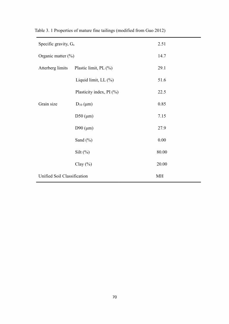
3.2 Properties of fine oil sand tailings ................................................................ 47
Page 6
vi
3.3 Standard Oedometer Test .............................................................................. 48
3.3.1 Experimental Apparatus .................................................................... 48
3.3.2 Testing Procedures ............................................................................ 49
3.3.3 Data Analysis .................................................................................... 50
3.3.4 Discussion ......................................................................................... 50
3.4 Falling Head Test .......................................................................................... 51
3.4.1 Experimental Apparatus .................................................................... 52
3.4.2 Testing Procedures ............................................................................ 52
3.4.3 Data Analysis .................................................................................... 53
3.4.4 Discussions ....................................................................................... 54
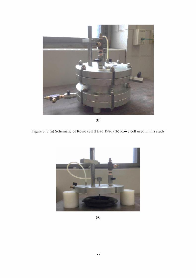
3.5 Rowe Cell Test .............................................................................................. 55
3.5.1 Experimental Apparatus .................................................................... 57
3.5.2 Testing Procedures ............................................................................ 59
3.5.3 Data analysis ..................................................................................... 66
3.5.4 Discussion ......................................................................................... 68
3.6 Summary ....................................................................................................... 68
CHAPTER 4 RESULTS AND DISCUSSIONS .......................................................... 83
4.1 Introduction ................................................................................................... 83
Page 7
vii
4.2 Laboratory Test Results ................................................................................ 84
4.2.1 Results of Standard Odometer Test ................................................... 84
4.2.2 Results of Falling Head Permeability Test ........................................ 85
4.2.3 Results of Rowe cell test ................................................................... 86
4.2.4 Discussions and Summary ................................................................ 87
4.3 A Comparison of the hydraulic conductivity data of oil sand tailings .......... 89
4.4 Regression Models for Fine Oil Sand Tailings ............................................. 93
4.4.1 Regression Models Based on the Experimental Results of this Study
.................................................................................................................... 94
4.4.2 Regression Models Based on the Database of Oil Sand Tailings ..... 96
4.4.3 Summary ........................................................................................... 97
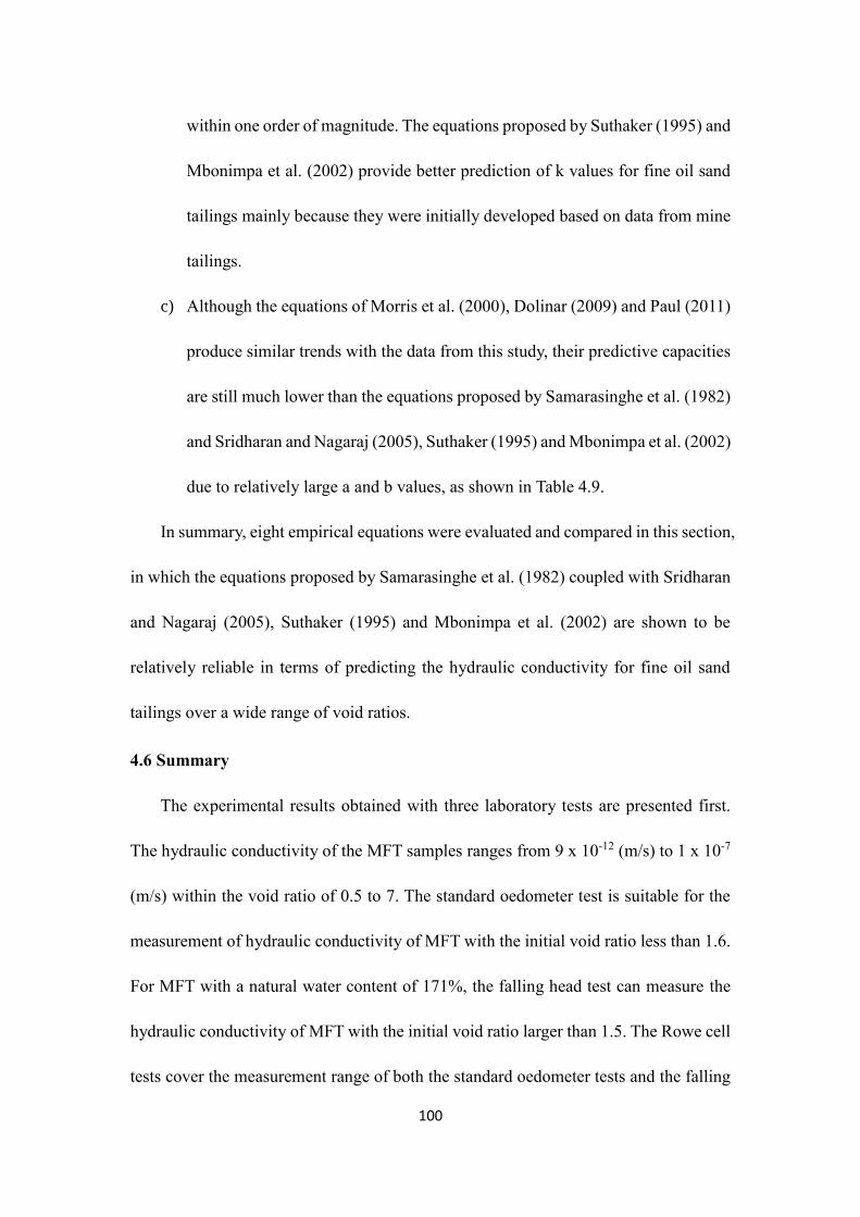
4.5 Evaluation and Comparison of Previous Empirical Equations ..................... 98
4.6 Summary ..................................................................................................... 100
CHAPTER 5 CONCLUSIONS AND RECOMMENDATIONS ............................... 128
5.1 Summary ..................................................................................................... 128
5.2 Conclusions ................................................................................................. 128
5.3 Engineering Significance ............................................................................ 130
5.4 Recommendations ....................................................................................... 130
Page 8
viii
BIBLIOGRAPHY ...................................................................................................... 132
LIST OF TABLES
CHAPTER 3
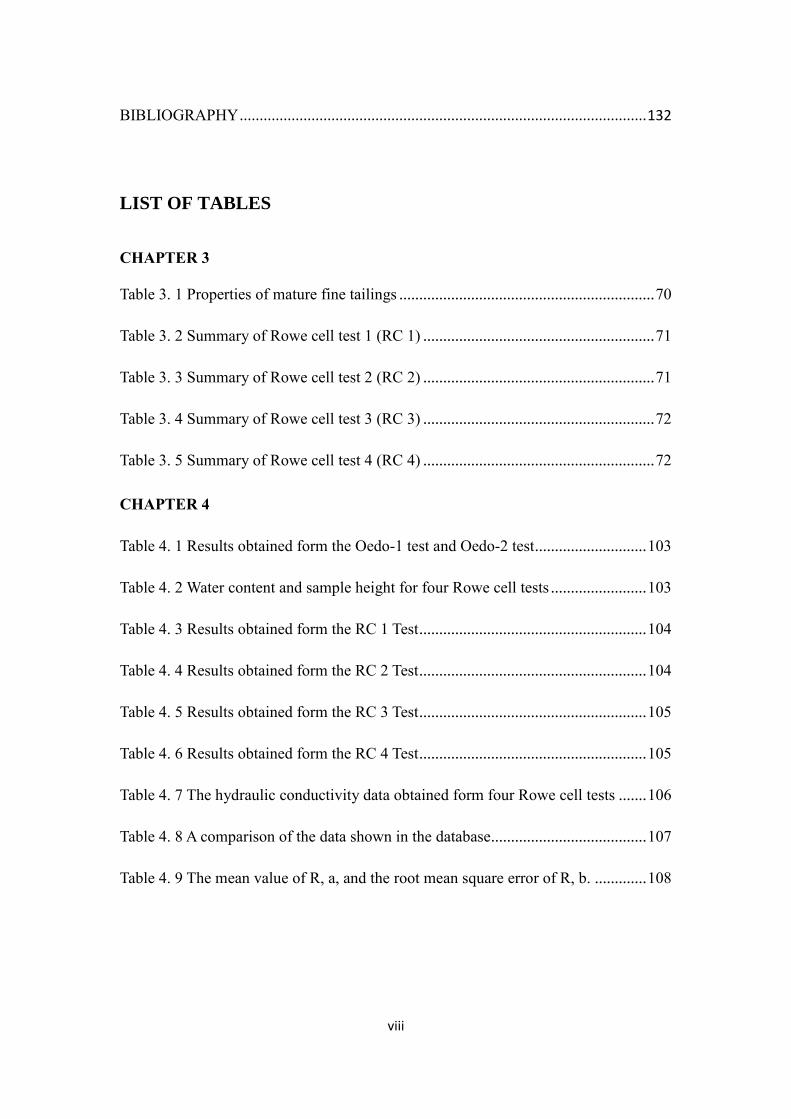
Table 3. 1 Properties of mature fine tailings ................................................................ 70
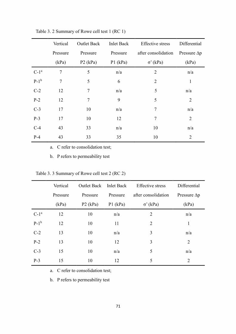
Table 3. 2 Summary of Rowe cell test 1 (RC 1) .......................................................... 71
Table 3. 3 Summary of Rowe cell test 2 (RC 2) .......................................................... 71
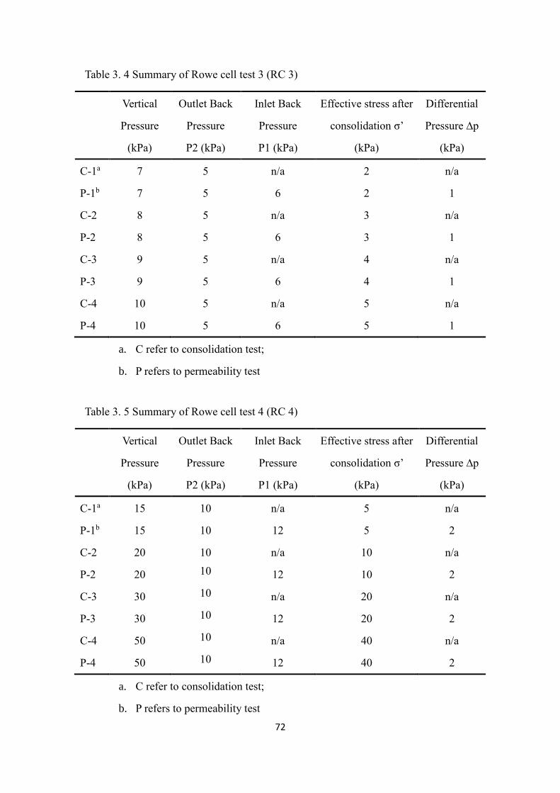
Table 3. 4 Summary of Rowe cell test 3 (RC 3) .......................................................... 72
Table 3. 5 Summary of Rowe cell test 4 (RC 4) .......................................................... 72
CHAPTER 4
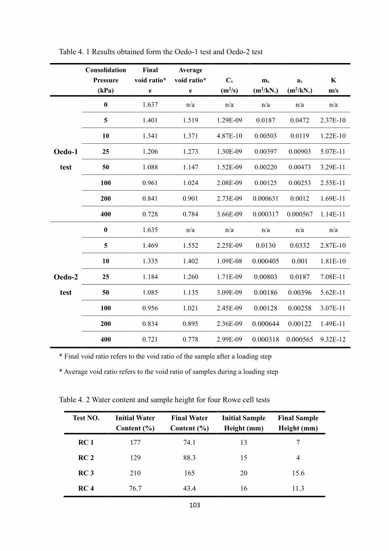
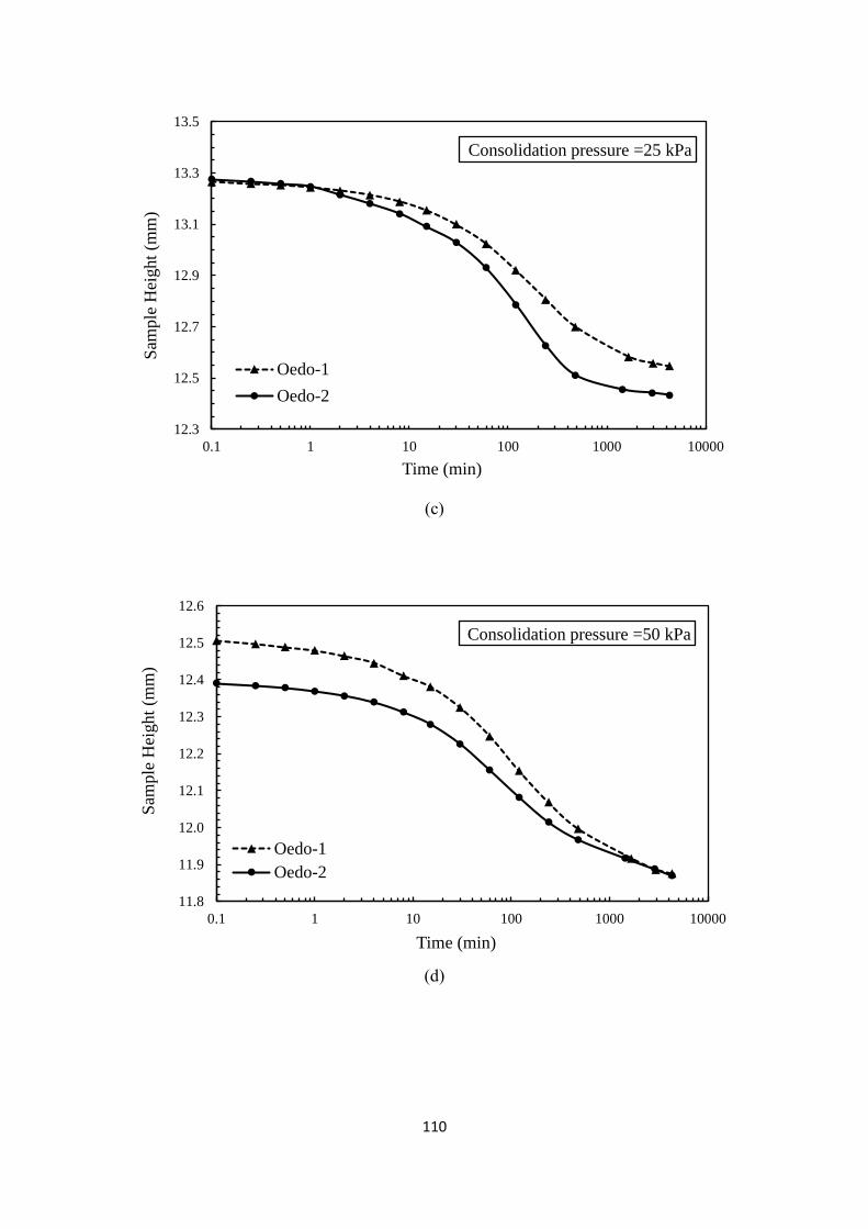
Table 4. 1 Results obtained form the Oedo-1 test and Oedo-2 test ............................ 103
Table 4. 2 Water content and sample height for four Rowe cell tests ........................ 103
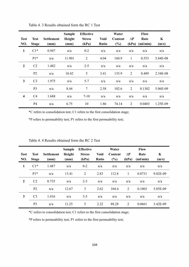
Table 4. 3 Results obtained form the RC 1 Test ......................................................... 104
Table 4. 4 Results obtained form the RC 2 Test ......................................................... 104
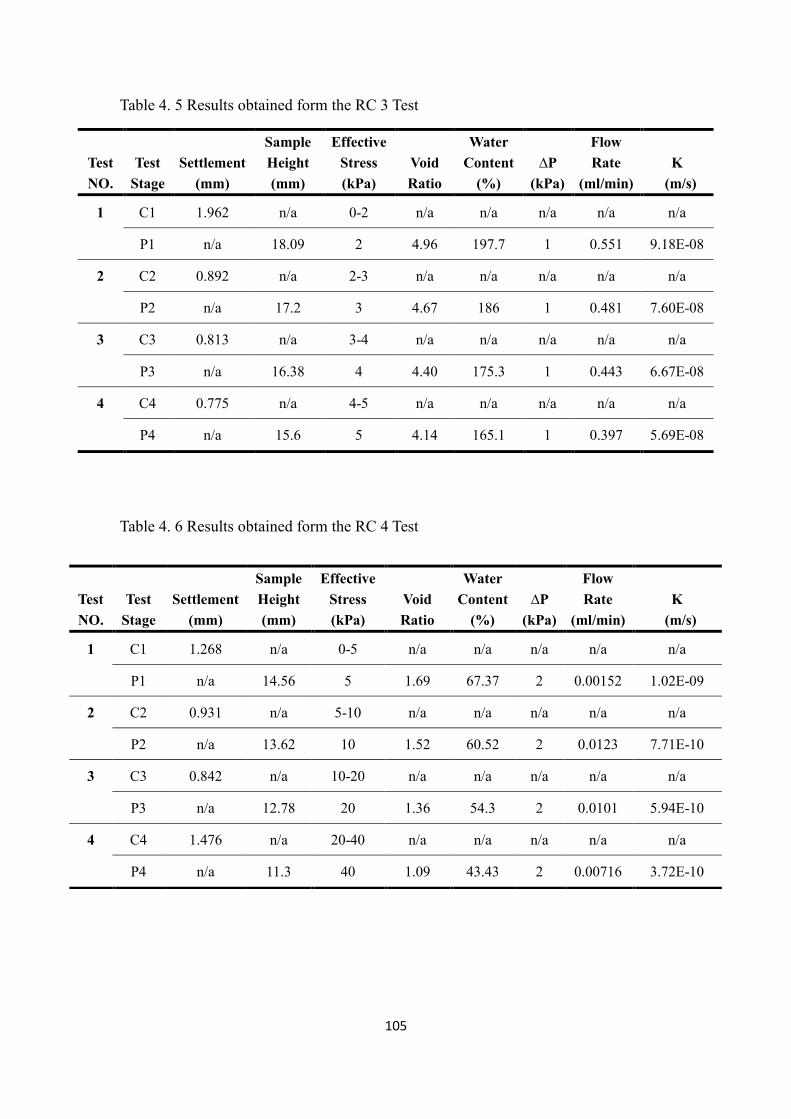
Table 4. 5 Results obtained form the RC 3 Test ......................................................... 105
Table 4. 6 Results obtained form the RC 4 Test ......................................................... 105
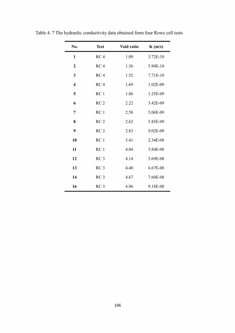
Table 4. 7 The hydraulic conductivity data obtained form four Rowe cell tests ....... 106
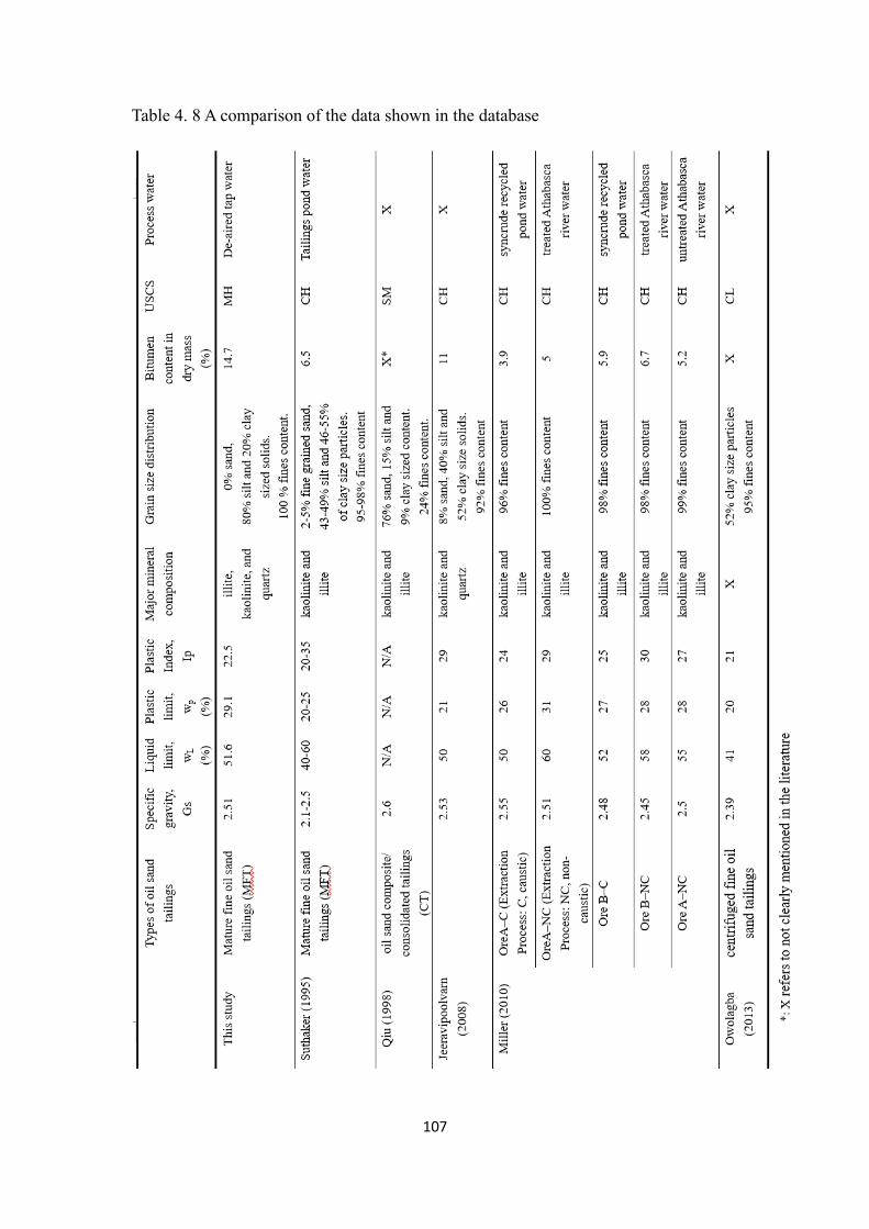
Table 4. 8 A comparison of the data shown in the database....................................... 107
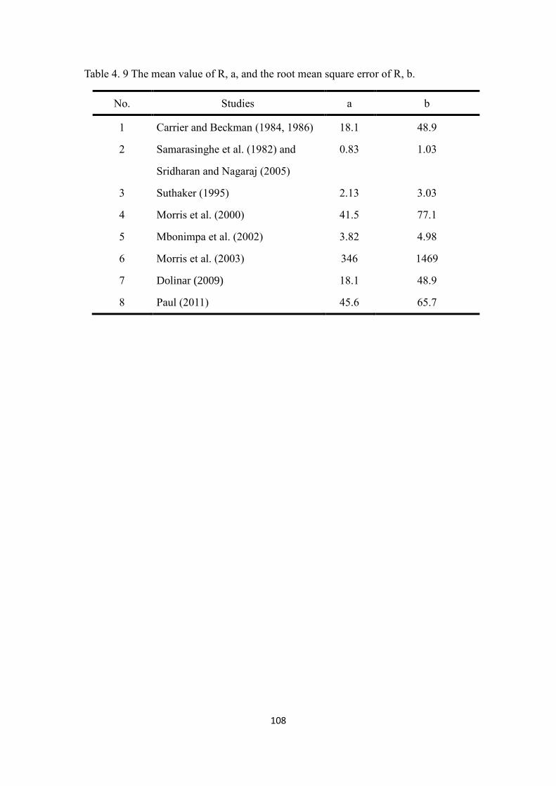
Table 4. 9 The mean value of R, a, and the root mean square error of R, b. ............. 108
Page 9
ix
LIST OF FIGURES
CHAPTER 2
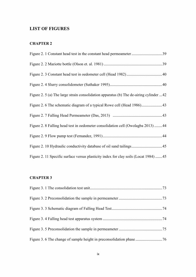
Figure 2. 1 Constant head test in the constant head permeameter ............................... 39
Figure 2. 2 Mariotte bottle (Olson et. al. 1981) ........................................................... 39
Figure 2. 3 Constant head test in oedometer cell (Head 1982) .................................... 40
Figure 2. 4 Slurry consolidometer (Suthaker 1995) ..................................................... 40
Figure 2. 5 (a) The large strain consolidation apparatus (b) The de-airing cylinder ... 42
Figure 2. 6 The schematic diagram of a typical Rowe cell (Head 1986) ..................... 43
Figure 2. 7 Falling Head Permeameter (Das, 2013) .................................................. 43
Figure 2. 8 Falling head test in oedometer consolidation cell (Owolagba 2013) ........ 44
Figure 2. 9 Flow pump test (Fernandez, 1991) ............................................................ 44
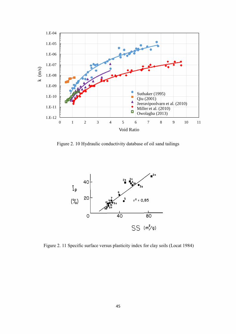
Figure 2. 10 Hydraulic conductivity database of oil sand tailings ............................... 45
Figure 2. 11 Specific surface versus plasticity index for clay soils (Locat 1984) ....... 45
CHAPTER 3
Figure 3. 1 The consolidation test unit ......................................................................... 73
Figure 3. 2 Preconsolidation the sample in permeameter ............................................ 73
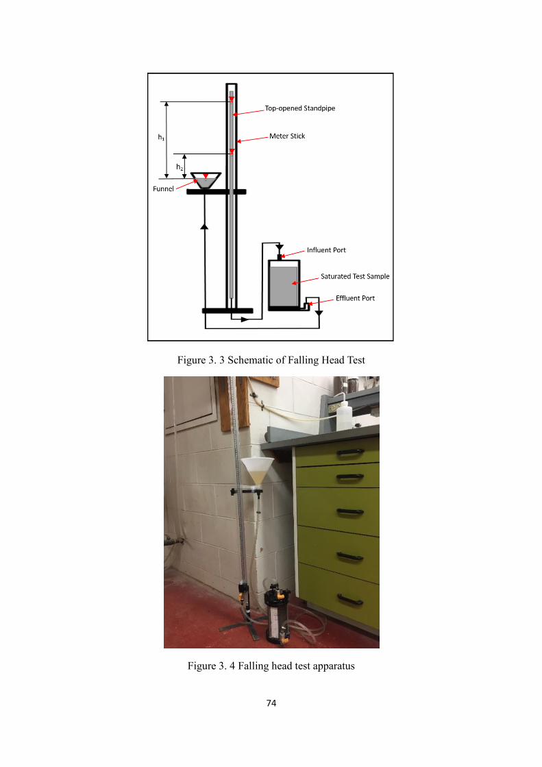
Figure 3. 3 Schematic diagram of Falling Head Test ................................................... 74
Figure 3. 4 Falling head test apparatus system ............................................................ 74
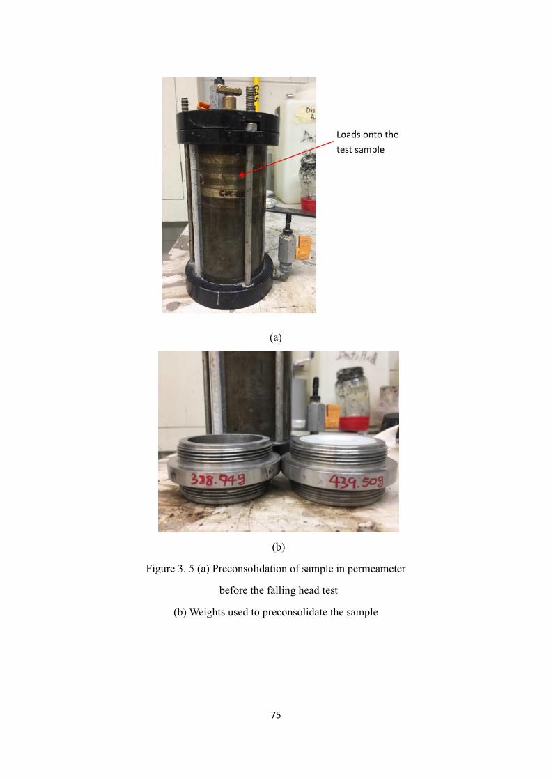
Figure 3. 5 Preconsolidation the sample in permeameter ............................................ 75
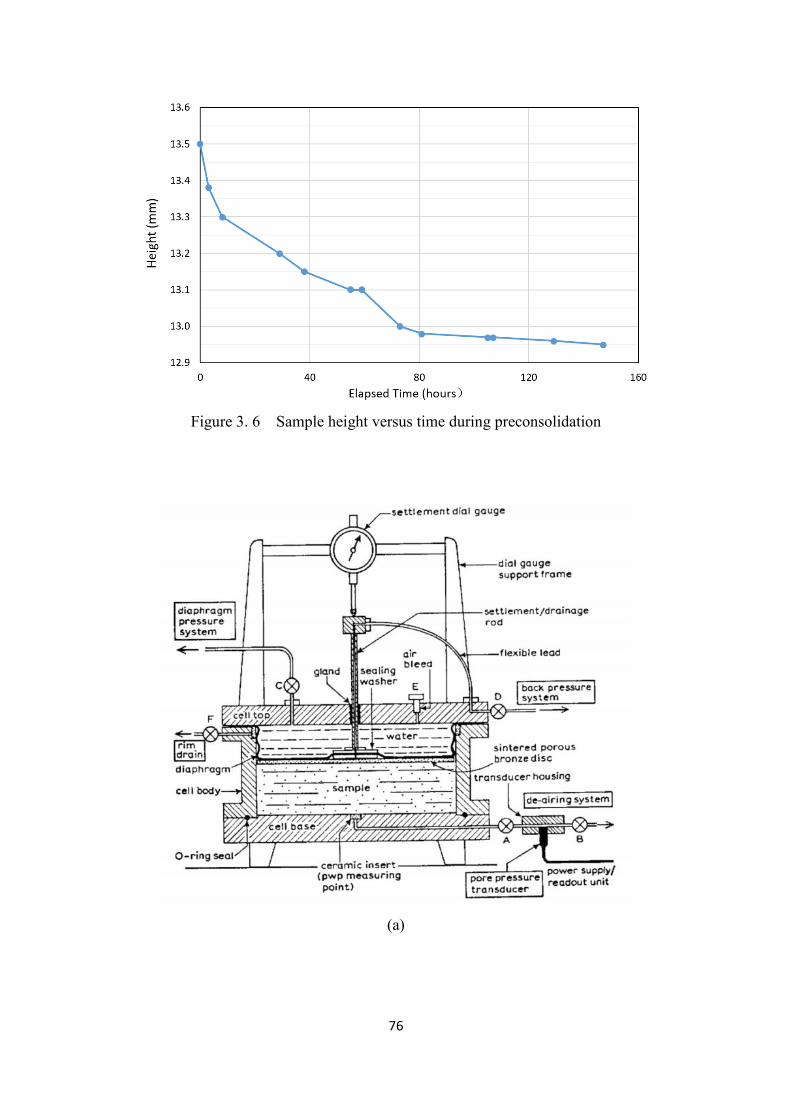
Figure 3. 6 The change of sample height in preconsolidation phase ........................... 76
Page 10
x
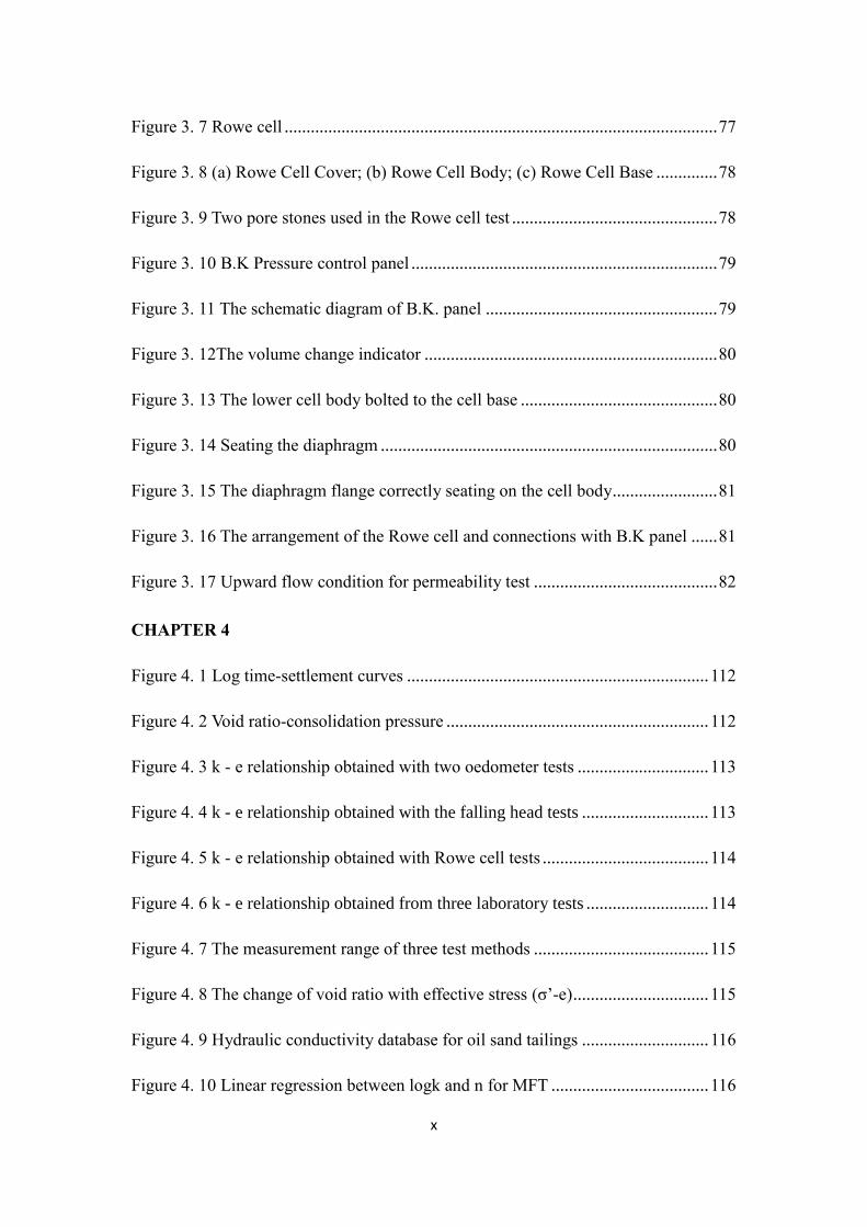
Figure 3. 7 Rowe cell ................................................................................................... 77
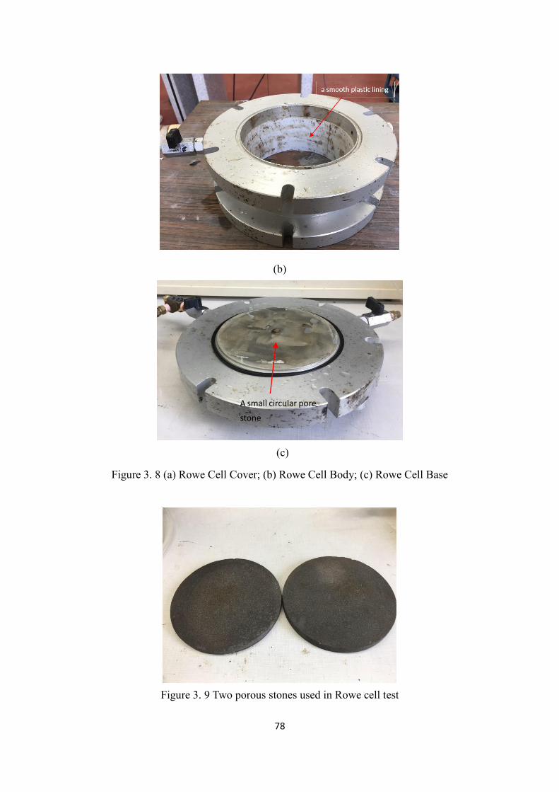
Figure 3. 8 (a) Rowe Cell Cover; (b) Rowe Cell Body; (c) Rowe Cell Base .............. 78
Figure 3. 9 Two pore stones used in the Rowe cell test ............................................... 78
Figure 3. 10 B.K Pressure control panel ...................................................................... 79
Figure 3. 11 The schematic diagram of B.K. panel ..................................................... 79
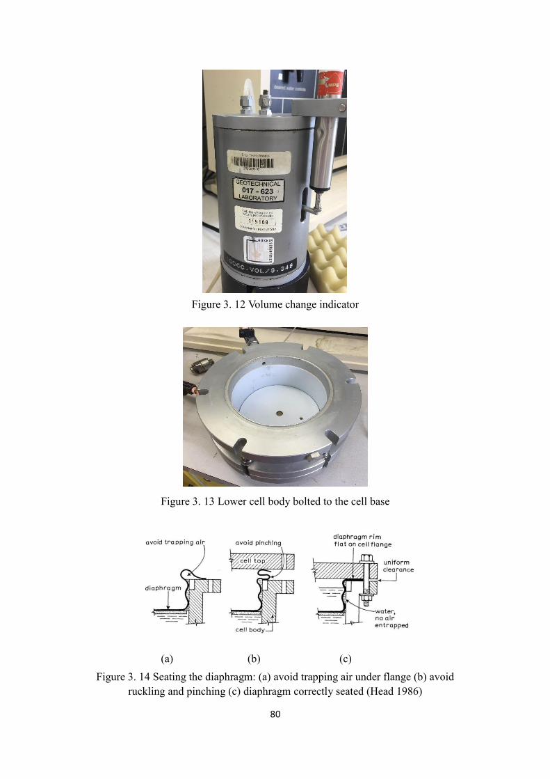
Figure 3. 12The volume change indicator ................................................................... 80
Figure 3. 13 The lower cell body bolted to the cell base ............................................. 80
Figure 3. 14 Seating the diaphragm ............................................................................. 80
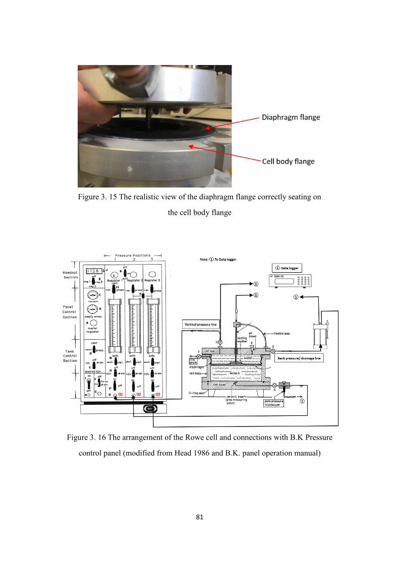
Figure 3. 15 The diaphragm flange correctly seating on the cell body ........................ 81
Figure 3. 16 The arrangement of the Rowe cell and connections with B.K panel ...... 81
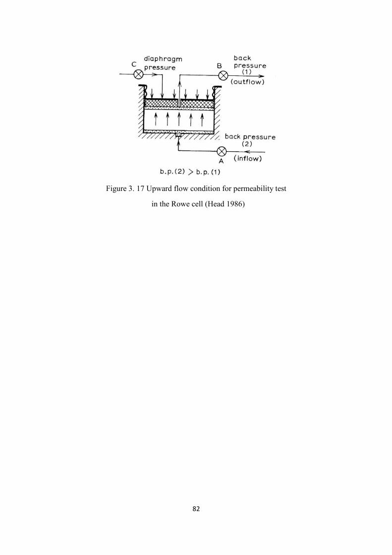
Figure 3. 17 Upward flow condition for permeability test .......................................... 82
CHAPTER 4
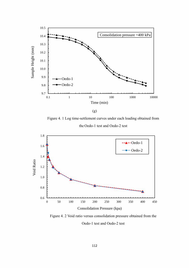
Figure 4. 1 Log time-settlement curves ..................................................................... 112
Figure 4. 2 Void ratio-consolidation pressure ............................................................ 112
Figure 4. 3 k - e relationship obtained with two oedometer tests .............................. 113
Figure 4. 4 k - e relationship obtained with the falling head tests ............................. 113
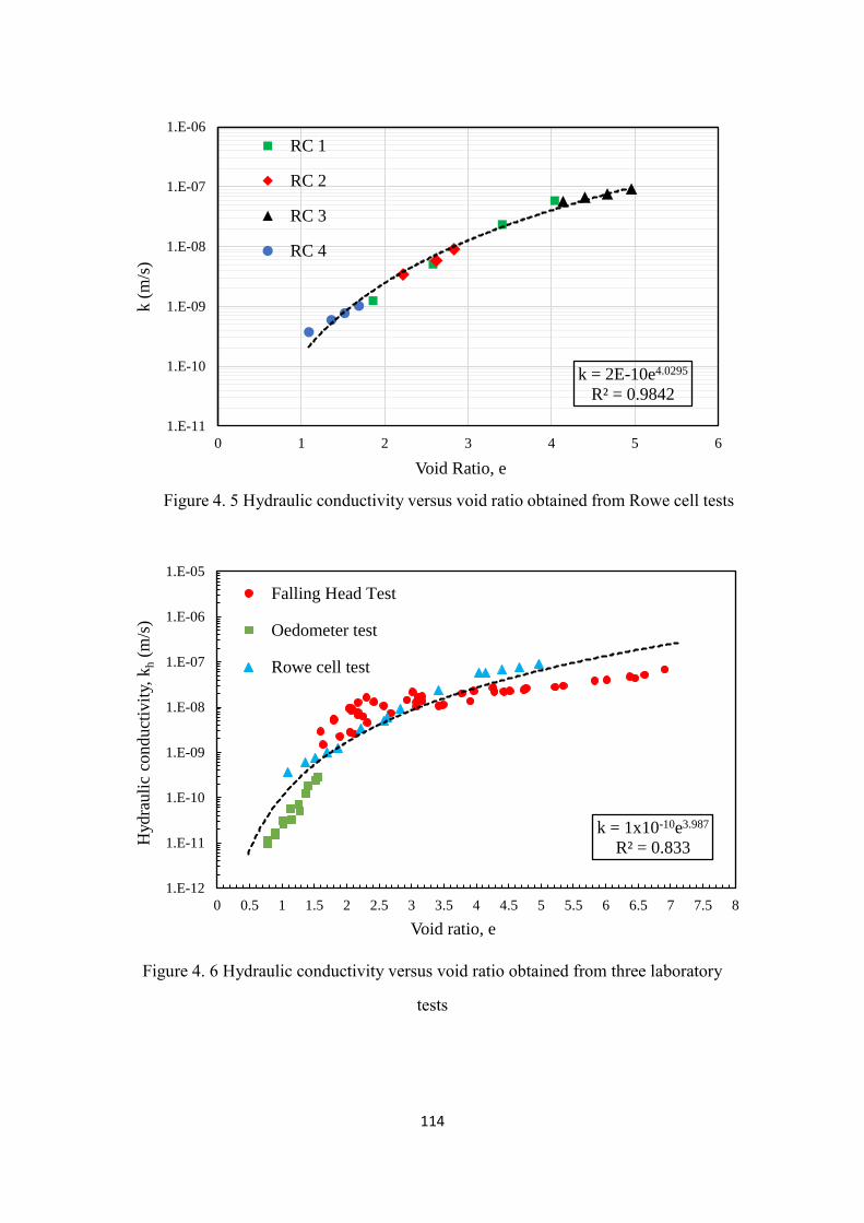
Figure 4. 5 k - e relationship obtained with Rowe cell tests ...................................... 114
Figure 4. 6 k - e relationship obtained from three laboratory tests ............................ 114
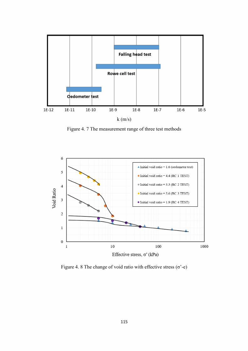
Figure 4. 7 The measurement range of three test methods ........................................ 115
Figure 4. 8 The change of void ratio with effective stress (σ’-e) ............................... 115
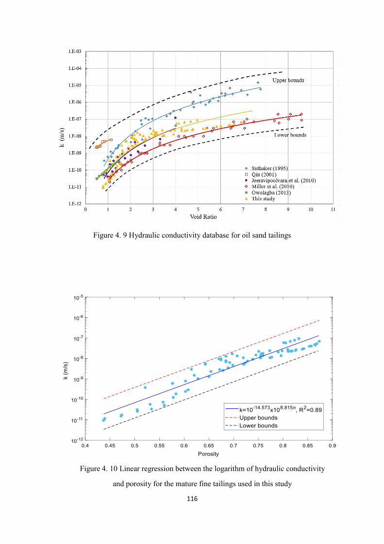
Figure 4. 9 Hydraulic conductivity database for oil sand tailings ............................. 116
Figure 4. 10 Linear regression between logk and n for MFT .................................... 116
Page 11
xi
Figure 4. 11 Linear regression between logk and e for oil sand tailings ................... 117
Figure 4. 12 Power regression between k and e for oil sand tailings ......................... 117
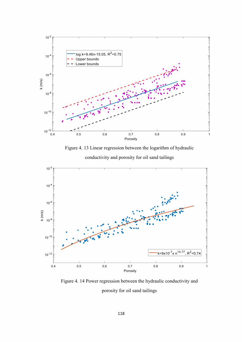
Figure 4. 13 Linear regression between logk and n for oil sand tailings ................... 118
Figure 4. 14 Power regression between k and n for oil sand tailings ........................ 118
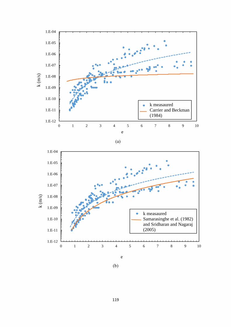
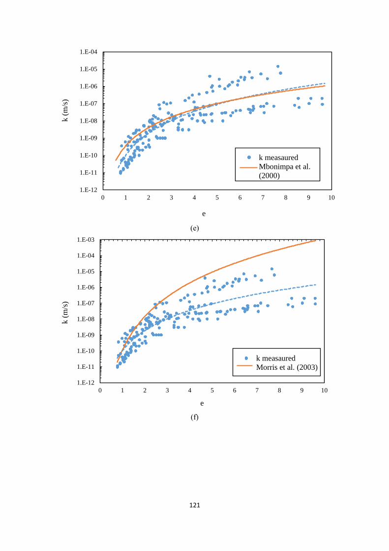
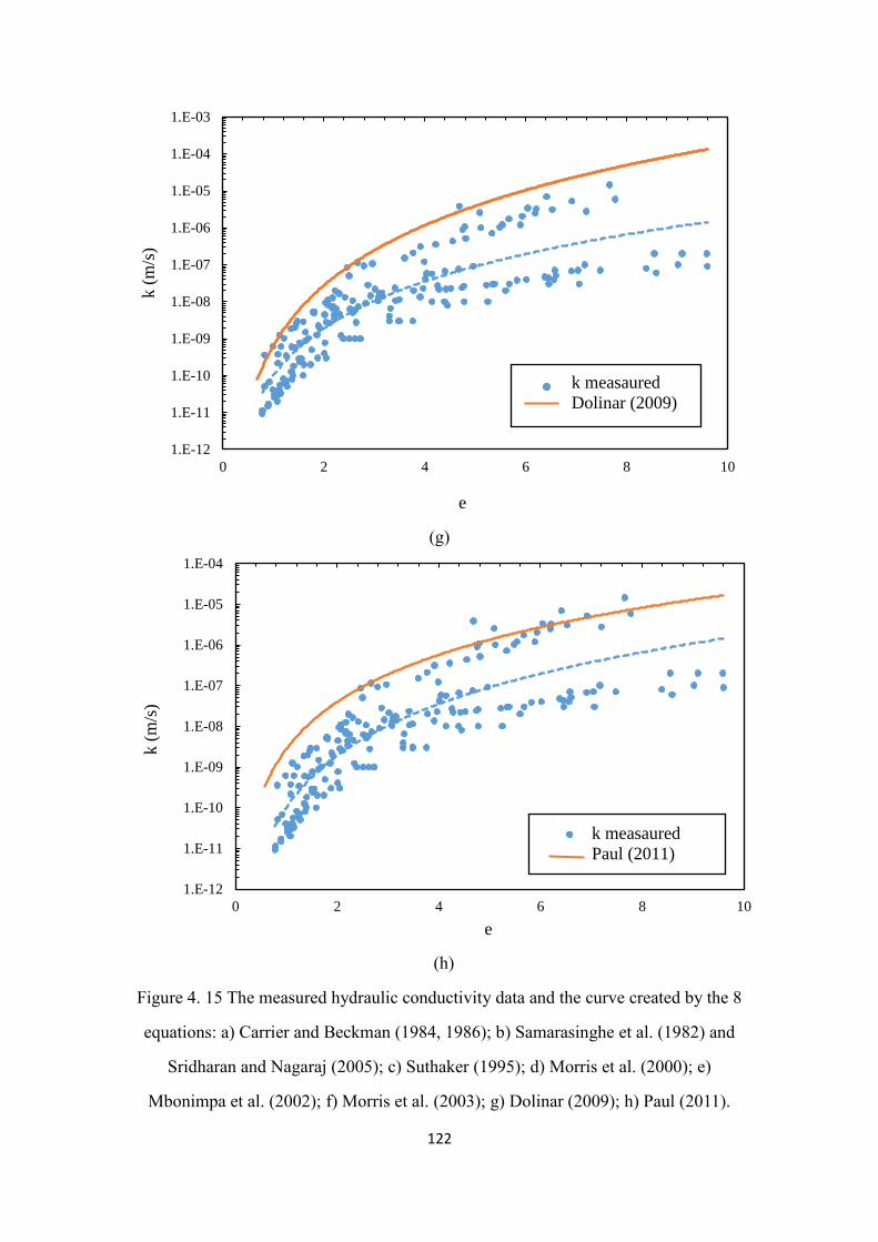
Figure 4. 15 The measured k data and the curves created by the 8 equations ........... 122
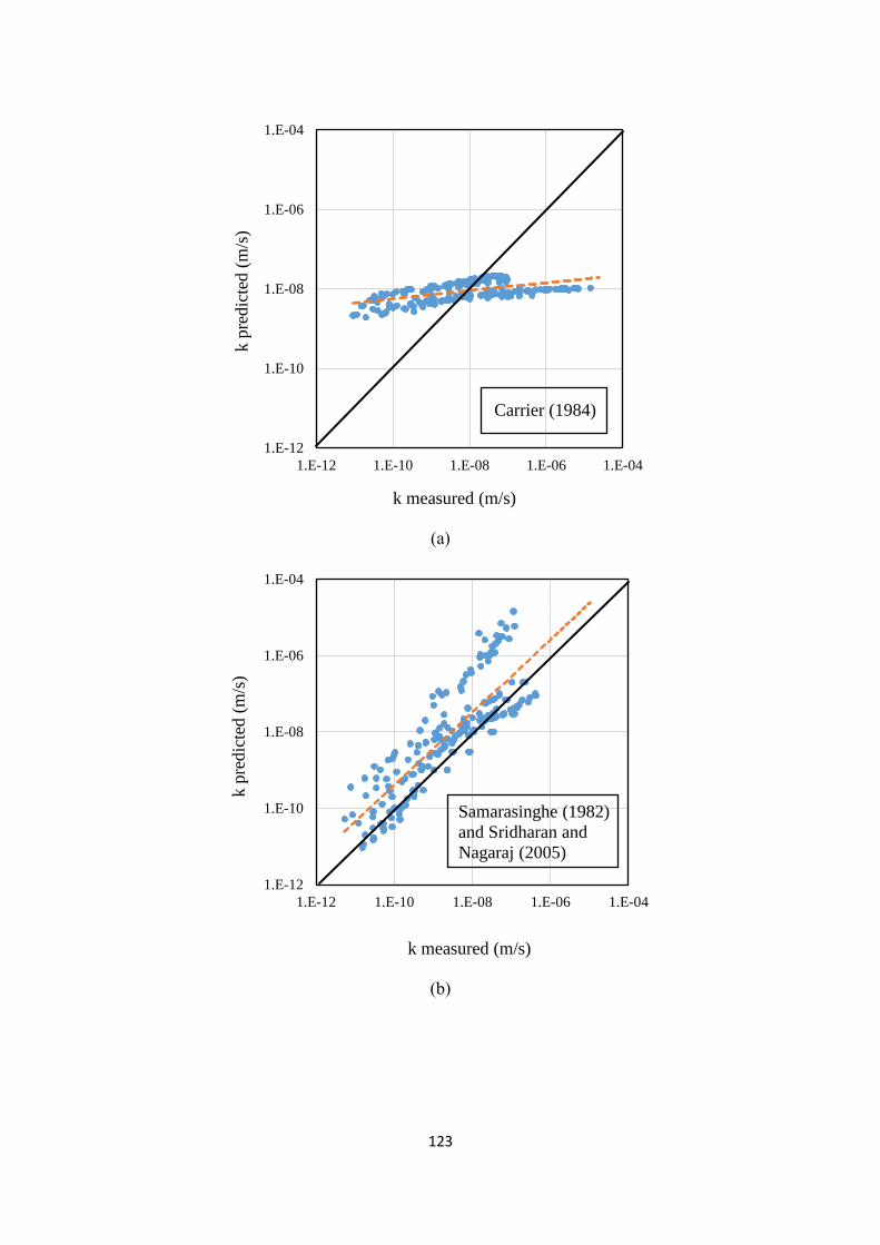
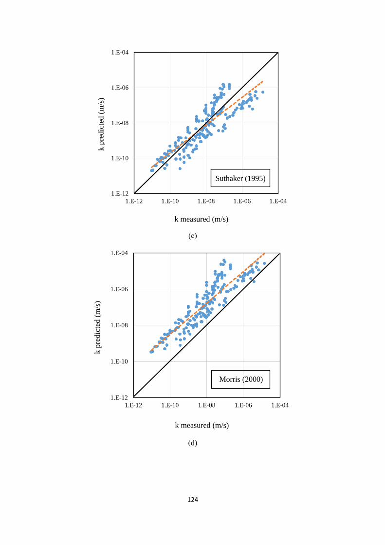
Figure 4. 16 kmeasured versus kpredicted calculated by the 8 equations.. .......................... 126
Page 12
xii
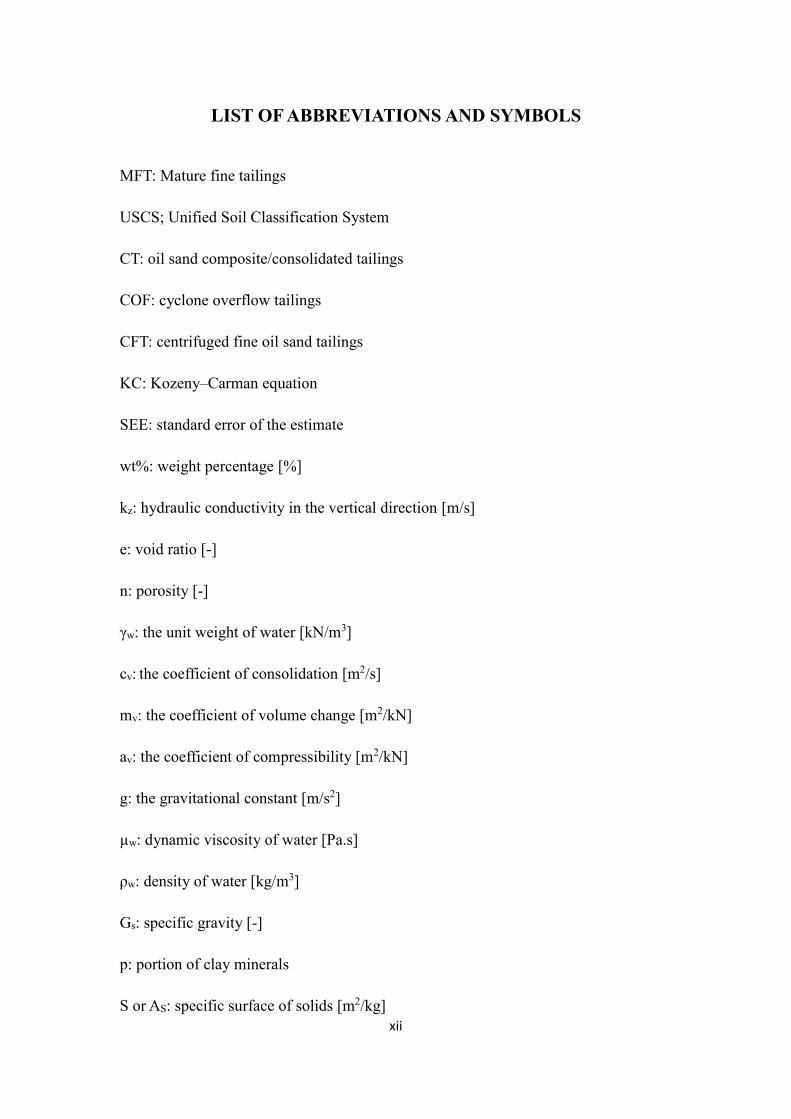
LIST OF ABBREVIATIONS AND SYMBOLS
MFT: Mature fine tailings
USCS; Unified Soil Classification System
CT: oil sand composite/consolidated tailings
COF: cyclone overflow tailings
CFT: centrifuged fine oil sand tailings
KC: Kozeny–Carman equation
SEE: standard error of the estimate
wt%: weight percentage [%]
kz: hydraulic conductivity in the vertical direction [m/s]
e: void ratio [-]
n: porosity [-]
γw: the unit weight of water [kN/m3]
cv: the coefficient of consolidation [m2/s]
mv: the coefficient of volume change [m2/kN]
av: the coefficient of compressibility [m2/kN]
g: the gravitational constant [m/s2]
µw: dynamic viscosity of water [Pa.s]
ρw: density of water [kg/m3]
Gs: specific gravity [-]
p: portion of clay minerals
S or AS: specific surface of solids [m2/kg]
Page 13
xiii
eL: the void ratio at liquid limit [-]
e/eL: the generalized state parameter [-]
r2: The coefficient of determination [-]
R: the ratio of a predicted value of k (kpredicted) to a measured value of k (kmeasured) [-]
a: mean value of R [-]
b: root mean square error of R [-]
Page 14
1
CHAPTER 1 INTRODUCTION
1.1 General
Oil sands mining processes produce tremendous amounts of tailings in northern
Alberta, Canada. The tailings are deposited to tailings ponds, where gravity segregation
takes place. During this process, sand settles more quickly than fine solids, which form
a stable suspension, called mature fine tailings (MFT). MFT typically consists of 90%
fines and stabilizes at a solids content of 30% (Jeeravipoolvarn 2010). Consolidation of
MFT is very slow because of the tailings’ low permeability (Jeeravipoolvarn 2010).
Management and treatment of the MFT are major challenges facing the oil sand industry.
Hydraulic conductivity is an important physical property of MFT because it
controls consolidation behaviors. Clear understandings of hydraulic conductivity and
its relationship with void ratio are essential to MFT management and treatment. Owing
to the excessive amount of time, and the sophisticated experimental techniques and
apparatus required, studies related to investigation and measurement of the hydraulic
conductivity over a wide range of void ratios for MFT are limited, and will be the focus
of this study.
1.2 Objectives of Study
The main objective of this study is to measure the hydraulic conductivity of MFT
over a relatively wide range of void ratios. The following specific objectives are devised:
• Existing experimental apparatuses and laboratory testing methods of the
measurement of hydraulic conductivity for fine grained geomaterials are
Page 15
2
summarized; particular attention is paid to the measurement methods for soft
fine-grained geomaterials, which have high water content and generally
present in the form of slurries.
• Available hydraulic conductivity data (k values) reported in the literature for
oil sand tailings are summarized. Particular attention is paid to k values of fine
grained oil sand tailings.
• Empirical equations proposed in previous studies to predict the hydraulic
conductivity for plastic soils are summarized.
• The hydraulic conductivity of MFT over a wide range of void ratios is
measured using three methods in laboratory tests, i.e. the standard oedometer
test, the falling head test and the Rowe cell test.
• Data regression models are developed to correlate the hydraulic conductivity
and a wide range of void ratios (k-e relationship) for fine oil sand tailings based
on data from this study as well as data published in the literature.
• The suitability and performances of empirical equations are assessed and
compared in terms of predicting hydraulic conductivity for fine oil sand tailings.
1.3 Thesis Outline
This thesis contains five chapters. Chapter 1 is an introduction of the thesis,
including the objective of this study, thesis outline and original contributions.
Chapter 2 presents the literature review, which primarily contains three parts: a
review of laboratory testing methods and relevant experimental apparatuses of the
measurement of hydraulic conductivity for fine grained geomaterials; a review of
Page 16
3
available hydraulic conductivity data for oil sand tailings; and a review of empirical
equations developed for the prediction of hydraulic conductivity of plastic soils.
Chapter 3 introduces the methodology of hydraulic conductivity measurement of
mature fine oil sand tailings (MFT). Geotechnical properties of MFT samples used in
this study are presented. The experimental apparatuses, testing procedures and data
analysis for the standard oedometer test, the falling head permeability test and Rowe
cell test are described in detail. The challenges associated with the sample preparation,
the test set up and execution, as well as limitations and possible sources of errors of the
laboratory test methods are reported.
Chapter 4 includes the analysis and discussions of experimental results obtained
from three laboratory testing methods. A hydraulic conductivity database for oil sand
tailings is established based on data from this study together with data published in the
literature. This database is used to develop the regression models, which correlate the
hydraulic conductivity with a wide range of void ratios for fine oil sand tailings. The
regression models proposed in this study can be used in the prediction and analysis of
the hydraulic conductivity for fine oil sand tailings. Selected empirical equations are
evaluated for their suitability and performances in predicting the hydraulic conductivity
for fine oil sand tailings.
Chapter 5 presents a summary of the thesis, conclusions and a recommendation for
future research.
1.4 Original Contributions
The original contributions of this study include:
Page 17
4
• Measuring the hydraulic conductivity for MFT over a wide range of void
ratios using three experimental devices
• Establishing a hydraulic conductivity database for oil sand tailings
• Developing data regression models for MFT and oil sand tailings
• Evaluating the suitability and performance of previous empirical equations
in terms of predicting hydraulic conductivity for fine oil sand tailings
Page 18
5
CHAPTER 2 LITERATURE REVIEW
2.1 Introduction
Oil sands tailings are by-products of the bitumen extraction process used in mining
operations. The tailings directly produced from oil sands processing are called whole
tailings.
The tailings slurry, which is discharged into a tailings pond for storage, contains
approximately 40% solids. Upon deposition, the tailings segregate, coarse solids settle
quickly, forming beaches. The remaining water, bitumen, and fines accumulate in the
center of tailings pond. Fine tailings remain suspended in the water and form a stable
suspension containing about 30 % solids and are known as mature fine tailings (Xu et.
al 2008). Compression of mature fine tailings (MFT) is extremely slow and MFT
remains in a fluid-like state for decades given the tailings’ low permeability
(Jeeravipoolvarn 2010). The management of tailings largely depends on the
consolidation behavior of MFT. Large volumes of MFT require multiple large
containment ponds, which generates environmental issues and leads to MFT
management challenges due to limited capacity of tailings pond.
The hydraulic conductivity is one of the most important physical properties of
geomaterials as it controls seepage and the rate of consolidation. In soil mechanics, the
hydraulic conductivity is defined as a coefficient of proportionality of Darcy’s law,
which links the discharge velocity with the hydraulic gradient. Darcy’s law can be
Page 19
6
expressed with the following equation (Das 2013):
v = ki (2.1)
where v[L/T] discharge velocity, i is hydraulic gradient, and k[L/T] is hydraulic
conductivity. Hence, the hydraulic conductivity can be measured through the volume
rate of flow, q[L3/T], and cross-sectional area, A[L2/T], given by the following equation:
q = kiA (2.2)
It should be noted that hydraulic conductivity is a measure of the rate of flow for a
particular fluid through a porous medium and its value varies as function of the fluid
and the porous medium. Permeability, also termed intrinsic permeability, is a property
of the medium itself and is not related to the fluid flowing through the fabric. The
hydraulic conductivity and permeability can be related by the following equation
(Adams 2011):
K g
k
(2.3)
where k [L/T] is the hydraulic conductivity, K[L2] is the intrinsic permeability, ρ [M/L3]
is the density of the fluid, g [L/T2] is the gravitational constant, and µ is the dynamic
viscosity [M/LT] which reflects one of the fluid properties.
Clear understanding of hydraulic conductivity and its relationship with void ratio
are essential to the investigation of the MFT consolidation behavior and oil sand tailings
Page 20
7
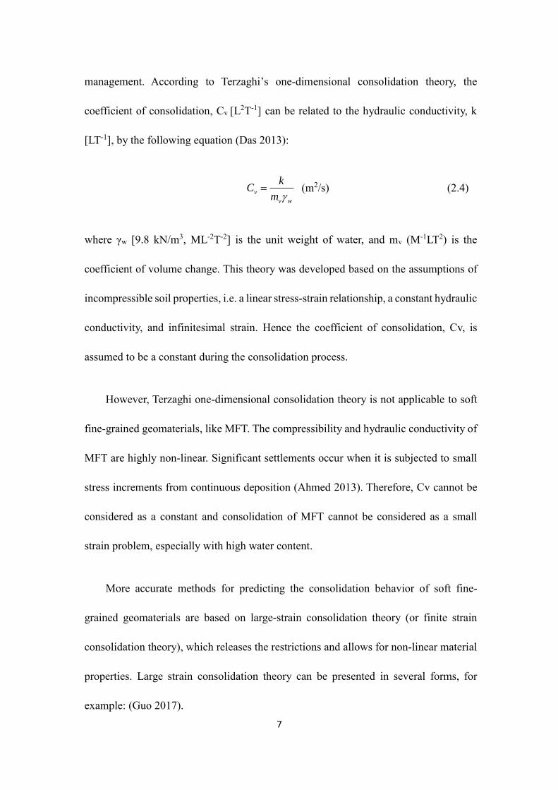
management. According to Terzaghi’s one-dimensional consolidation theory, the
coefficient of consolidation, Cv [L2T-1] can be related to the hydraulic conductivity, k
[LT-1], by the following equation (Das 2013):
v
v w
kC
m (m2/s) (2.4)
where γw [9.8 kN/m3, ML-2T-2] is the unit weight of water, and mv (M-1LT2) is the
coefficient of volume change. This theory was developed based on the assumptions of
incompressible soil properties, i.e. a linear stress-strain relationship, a constant hydraulic
conductivity, and infinitesimal strain. Hence the coefficient of consolidation, Cv, is
assumed to be a constant during the consolidation process.
However, Terzaghi one-dimensional consolidation theory is not applicable to soft
fine-grained geomaterials, like MFT. The compressibility and hydraulic conductivity of
MFT are highly non-linear. Significant settlements occur when it is subjected to small
stress increments from continuous deposition (Ahmed 2013). Therefore, Cv cannot be
considered as a constant and consolidation of MFT cannot be considered as a small
strain problem, especially with high water content.
More accurate methods for predicting the consolidation behavior of soft fine-
grained geomaterials are based on large-strain consolidation theory (or finite strain
consolidation theory), which releases the restrictions and allows for non-linear material
properties. Large strain consolidation theory can be presented in several forms, for
example: (Guo 2017).
Page 21
8
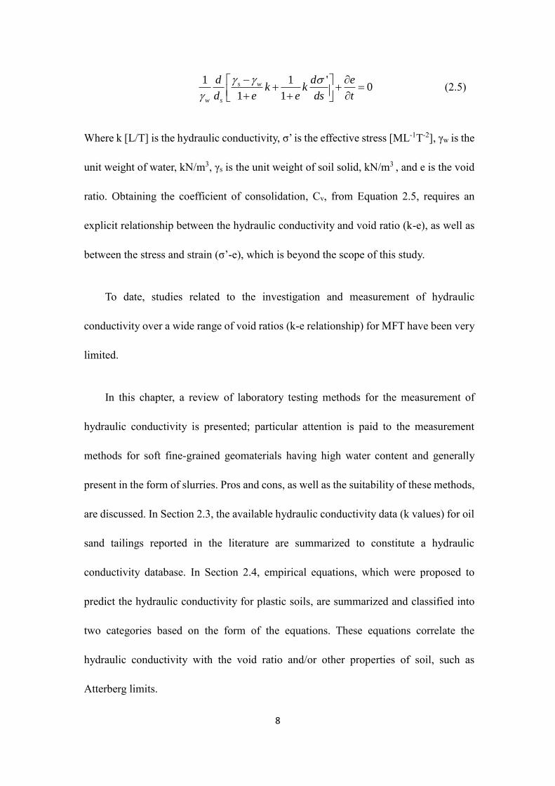
1 1 '
01 1
s w
w s
d d ek k
d e e ds t
(2.5)
Where k [L/T] is the hydraulic conductivity, σ’ is the effective stress [ML-1T-2], γw is the
unit weight of water, kN/m3, γs is the unit weight of soil solid, kN/m3 , and e is the void
ratio. Obtaining the coefficient of consolidation, Cv, from Equation 2.5, requires an
explicit relationship between the hydraulic conductivity and void ratio (k-e), as well as
between the stress and strain (σ’-e), which is beyond the scope of this study.
To date, studies related to the investigation and measurement of hydraulic
conductivity over a wide range of void ratios (k-e relationship) for MFT have been very
limited.
In this chapter, a review of laboratory testing methods for the measurement of
hydraulic conductivity is presented; particular attention is paid to the measurement
methods for soft fine-grained geomaterials having high water content and generally
present in the form of slurries. Pros and cons, as well as the suitability of these methods,
are discussed. In Section 2.3, the available hydraulic conductivity data (k values) for oil
sand tailings reported in the literature are summarized to constitute a hydraulic
conductivity database. In Section 2.4, empirical equations, which were proposed to
predict the hydraulic conductivity for plastic soils, are summarized and classified into
two categories based on the form of the equations. These equations correlate the
hydraulic conductivity with the void ratio and/or other properties of soil, such as
Atterberg limits.
Page 22
9
2.2 Laboratory Methods and Apparatuses of the Hydraulic Conductivity
Measurement
Many techniques and methods have been developed and reported in previous
studies to measure the hydraulic conductivity of soils in the laboratory. In this section,
existing experimental apparatuses and testing methods of the hydraulic conductivity
measurement in the laboratory are summarized. For fine-grained soils with high-water
content, conventional measurement techniques are inadequate or even not suitable for
determining the hydraulic conductivity. Therefore, special attention is paid to
experimental apparatuses and methods designed for soft fine-grained geomaterials that
have a high compressibility and low permeability.
The hydraulic conductivity of soils can be measured by direct or indirect methods.
In sections 2.2.1 and 2.2.2, two types of methods are introduced, and a comparison
between the direct and indirect methods is presented in Section 2.2.3.
2.2.1 Direct Methods
2.2.1.1 Constant Head Test
The constant head test has been carried out in various apparatuses, such as the
constant head permeameter, the oedometer cell, the slurry consolidometer, the large
strain consolidation cell and the Rowe cell, to directly measure the hydraulic
conductivity of geomaterials. In this section, these appartuses are introduced in detail.
It should be noted that the test performed in constant head permeameter is a standarad
Page 23
10
test followed by standard ASTM D2434, except which the test performed in other
apparatuses mentioned above are non-standard tests.
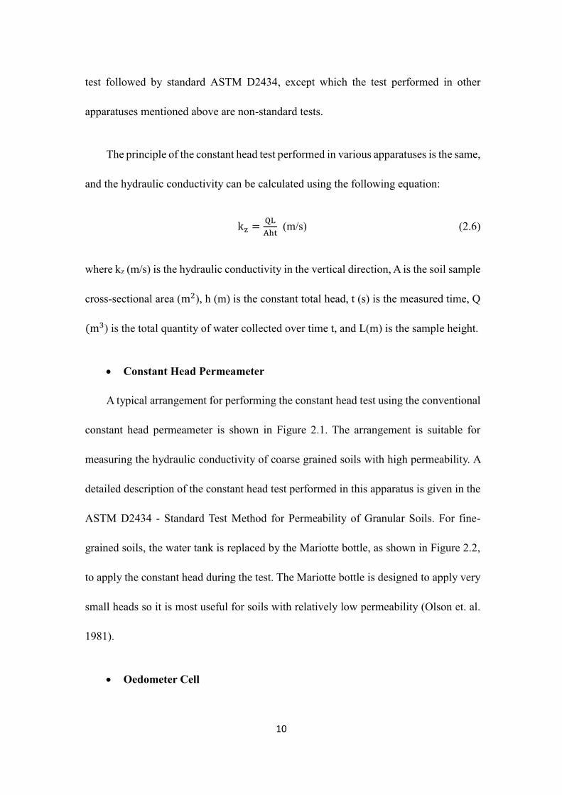
The principle of the constant head test performed in various apparatuses is the same,
and the hydraulic conductivity can be calculated using the following equation:
kz =QL
Aht (m/s) (2.6)
where kz (m/s) is the hydraulic conductivity in the vertical direction, A is the soil sample
cross-sectional area (m2), h (m) is the constant total head, t (s) is the measured time, Q
(m3) is the total quantity of water collected over time t, and L(m) is the sample height.
• Constant Head Permeameter
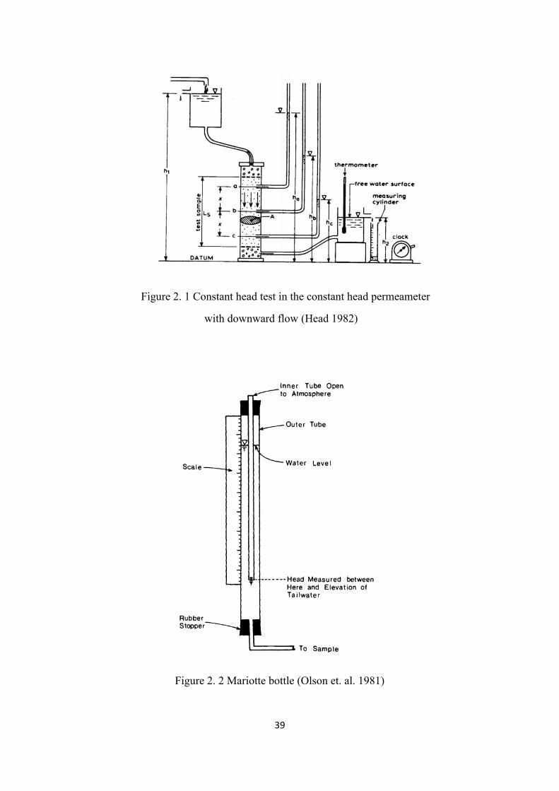
A typical arrangement for performing the constant head test using the conventional
constant head permeameter is shown in Figure 2.1. The arrangement is suitable for
measuring the hydraulic conductivity of coarse grained soils with high permeability. A
detailed description of the constant head test performed in this apparatus is given in the
ASTM D2434 - Standard Test Method for Permeability of Granular Soils. For fine-
grained soils, the water tank is replaced by the Mariotte bottle, as shown in Figure 2.2,
to apply the constant head during the test. The Mariotte bottle is designed to apply very
small heads so it is most useful for soils with relatively low permeability (Olson et. al.
1981).
• Oedometer Cell
Page 24
11
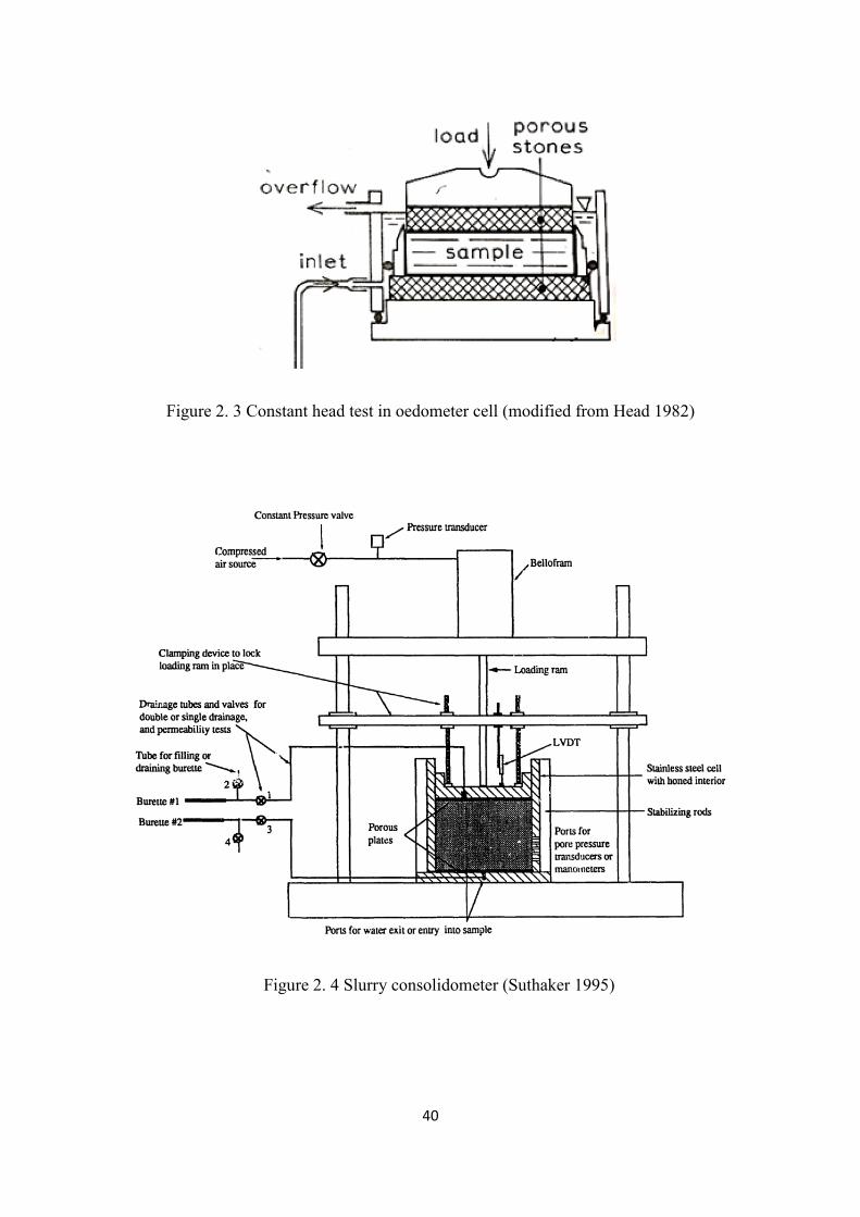
Some oedometer cells are equipped with the means to perform the constant head
test while the sample is under load, as shown in Figure 2.3. The essential features of
such oedometer cells are a bottom inlet, which can be connected to a standpipe; sealing
rings to prevent water escaping around the specimen and containing ring; and an upper
overflow outlet (Head 1982).
The constant head test performed in such an oedometer cell is more suitable for
soils with intermediate permeability, such as silts. However, this method cannot be used
for soft fine-grained geomaterials with high initial water content because large
deformations occur during the consolidation stage, so the small sample thickness is not
adequate for consolidation.
• Slurry Consolidometer
Figure 2.4 shows the slurry consolidometer, which was developed in the
Geotechnical Centre at the University of Alberta, to carry out large strain consolidation
tests (Jeeravipoolvarn 2005). The slurry consolidometer is about 30 cm in height and 20
cm in diameter, which allows large deformation during the consolidation and allows the
constant head test to be directly performed at the end of each consolidation loading step.
This apparatus is equipped with a clamping device, which consists of a horizontal steel
bar (50 mm by 50 mm) fastened to two vertical frame rods, to prevent settlements caused
by the applied hydraulic gradients when performing permeability tests on slurry-like
soils (Suthaker 1995).
Page 25
12
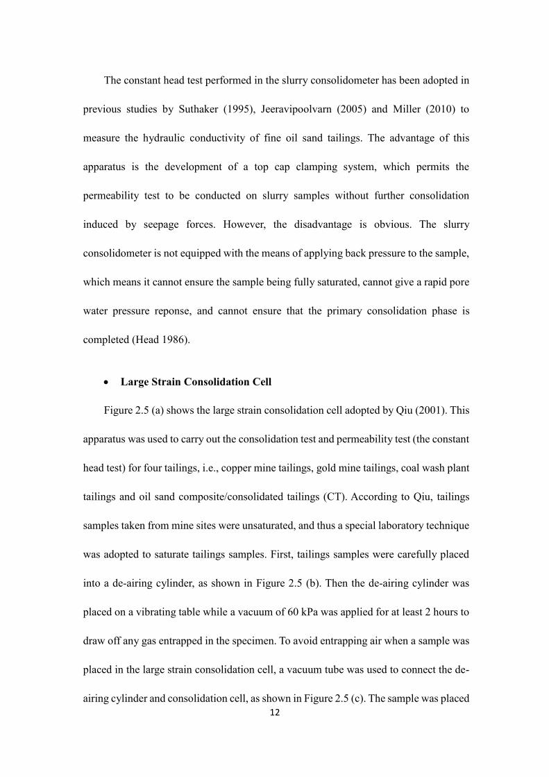
The constant head test performed in the slurry consolidometer has been adopted in
previous studies by Suthaker (1995), Jeeravipoolvarn (2005) and Miller (2010) to
measure the hydraulic conductivity of fine oil sand tailings. The advantage of this
apparatus is the development of a top cap clamping system, which permits the
permeability test to be conducted on slurry samples without further consolidation
induced by seepage forces. However, the disadvantage is obvious. The slurry
consolidometer is not equipped with the means of applying back pressure to the sample,
which means it cannot ensure the sample being fully saturated, cannot give a rapid pore
water pressure reponse, and cannot ensure that the primary consolidation phase is
completed (Head 1986).
• Large Strain Consolidation Cell
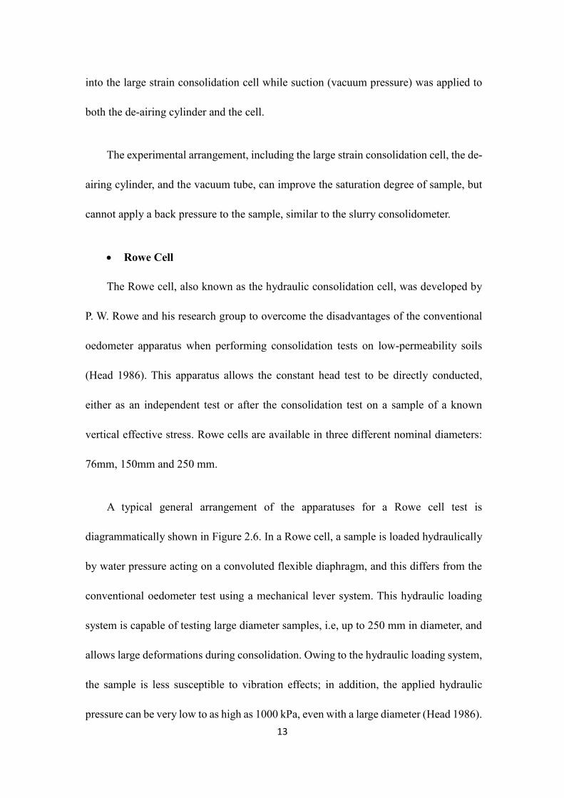
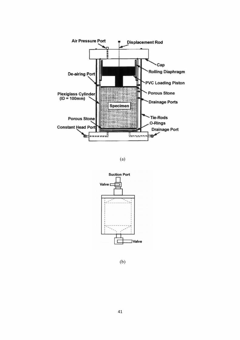
Figure 2.5 (a) shows the large strain consolidation cell adopted by Qiu (2001). This
apparatus was used to carry out the consolidation test and permeability test (the constant
head test) for four tailings, i.e., copper mine tailings, gold mine tailings, coal wash plant
tailings and oil sand composite/consolidated tailings (CT). According to Qiu, tailings
samples taken from mine sites were unsaturated, and thus a special laboratory technique
was adopted to saturate tailings samples. First, tailings samples were carefully placed
into a de-airing cylinder, as shown in Figure 2.5 (b). Then the de-airing cylinder was
placed on a vibrating table while a vacuum of 60 kPa was applied for at least 2 hours to
draw off any gas entrapped in the specimen. To avoid entrapping air when a sample was
placed in the large strain consolidation cell, a vacuum tube was used to connect the de-
airing cylinder and consolidation cell, as shown in Figure 2.5 (c). The sample was placed
Page 26
13
into the large strain consolidation cell while suction (vacuum pressure) was applied to
both the de-airing cylinder and the cell.
The experimental arrangement, including the large strain consolidation cell, the de-
airing cylinder, and the vacuum tube, can improve the saturation degree of sample, but
cannot apply a back pressure to the sample, similar to the slurry consolidometer.
• Rowe Cell
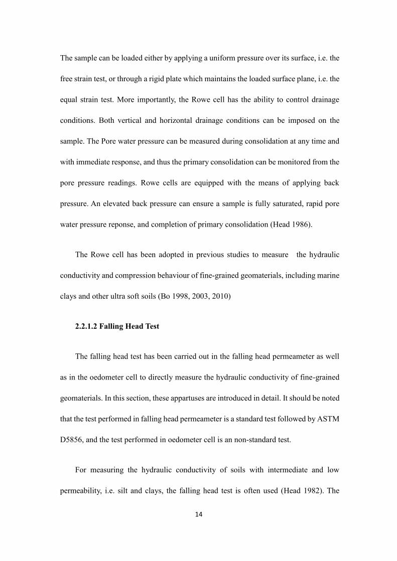
The Rowe cell, also known as the hydraulic consolidation cell, was developed by
P. W. Rowe and his research group to overcome the disadvantages of the conventional
oedometer apparatus when performing consolidation tests on low-permeability soils
(Head 1986). This apparatus allows the constant head test to be directly conducted,
either as an independent test or after the consolidation test on a sample of a known
vertical effective stress. Rowe cells are available in three different nominal diameters:
76mm, 150mm and 250 mm.
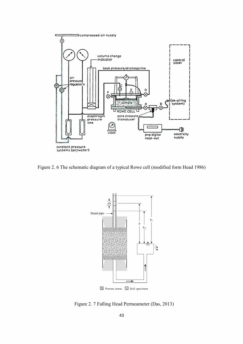
A typical general arrangement of the apparatuses for a Rowe cell test is
diagrammatically shown in Figure 2.6. In a Rowe cell, a sample is loaded hydraulically
by water pressure acting on a convoluted flexible diaphragm, and this differs from the
conventional oedometer test using a mechanical lever system. This hydraulic loading
system is capable of testing large diameter samples, i.e, up to 250 mm in diameter, and
allows large deformations during consolidation. Owing to the hydraulic loading system,
the sample is less susceptible to vibration effects; in addition, the applied hydraulic
pressure can be very low to as high as 1000 kPa, even with a large diameter (Head 1986).
Page 27
14
The sample can be loaded either by applying a uniform pressure over its surface, i.e. the
free strain test, or through a rigid plate which maintains the loaded surface plane, i.e. the
equal strain test. More importantly, the Rowe cell has the ability to control drainage
conditions. Both vertical and horizontal drainage conditions can be imposed on the
sample. The Pore water pressure can be measured during consolidation at any time and
with immediate response, and thus the primary consolidation can be monitored from the
pore pressure readings. Rowe cells are equipped with the means of applying back
pressure. An elevated back pressure can ensure a sample is fully saturated, rapid pore
water pressure reponse, and completion of primary consolidation (Head 1986).
The Rowe cell has been adopted in previous studies to measure the hydraulic
conductivity and compression behaviour of fine-grained geomaterials, including marine
clays and other ultra soft soils (Bo 1998, 2003, 2010)
2.2.1.2 Falling Head Test
The falling head test has been carried out in the falling head permeameter as well
as in the oedometer cell to directly measure the hydraulic conductivity of fine-grained
geomaterials. In this section, these appartuses are introduced in detail. It should be noted
that the test performed in falling head permeameter is a standard test followed by ASTM
D5856, and the test performed in oedometer cell is an non-standard test.
For measuring the hydraulic conductivity of soils with intermediate and low
permeability, i.e. silt and clays, the falling head test is often used (Head 1982). The
Page 28
15
principle of the falling head test performed in various apparatuses is basically the same,
i.e. a soil sample is connected to a standpipe which provides both the head of water and
the means of measuring the quantity of water flowing through the sample (Head 1982).
Denoting the cross-sectional area of the standpipe by a (m2), sample length by L (m),
sample cross-sectional area by A (m2), time duration by t (s), and h1 (m) and h2 (m) are
initial and final hydraulic head differences, respectively, the vertical hydraulic
conductivity k (m/s) can be determined using the following equation (Budhu 2007):
1
2
lnhaL
kAt h
(m/s) (2.7)
• Falling Head Permeameter
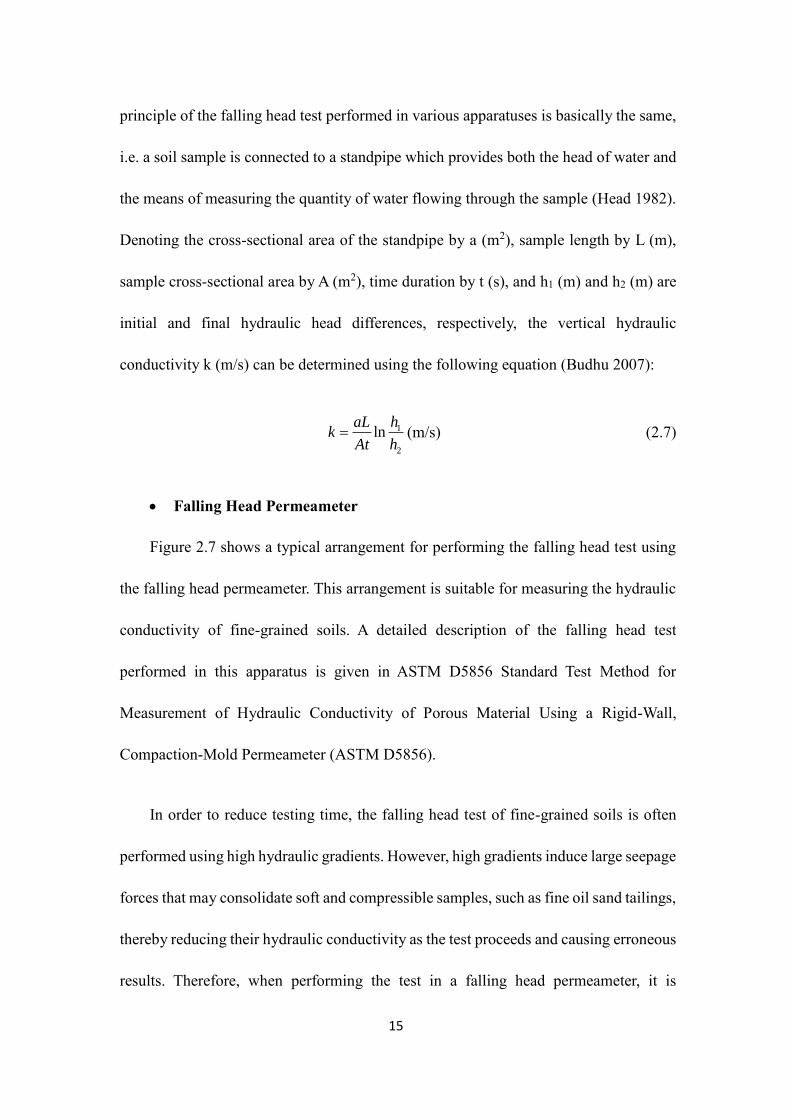
Figure 2.7 shows a typical arrangement for performing the falling head test using
the falling head permeameter. This arrangement is suitable for measuring the hydraulic
conductivity of fine-grained soils. A detailed description of the falling head test
performed in this apparatus is given in ASTM D5856 Standard Test Method for
Measurement of Hydraulic Conductivity of Porous Material Using a Rigid-Wall,
Compaction-Mold Permeameter (ASTM D5856).
In order to reduce testing time, the falling head test of fine-grained soils is often
performed using high hydraulic gradients. However, high gradients induce large seepage
forces that may consolidate soft and compressible samples, such as fine oil sand tailings,
thereby reducing their hydraulic conductivity as the test proceeds and causing erroneous
results. Therefore, when performing the test in a falling head permeameter, it is
Page 29
16
important to apply an appropriate hydraulic gradient to the sample without causing
significant consolidation, particularly for soft fine-grained samples with high water
contents, and to avoid prolonged testing time.
• Oedometer Cell
The falling head test can be performed in the oedometer cell at various stages during
a consolidation test after the completion of the primary consolidation. An oedometer cell
arranged for the falling head test with an upward flow is shown in Figure 2.8, which is
similar to the constant head test performed in the oedometer cell. The test is started by
opening the pinch clip (shown in Figure 2.8) and running the clock when the level in the
burette reaches the first desired level. The next step is to record the time taken to the
level in the burette to fall to the second desired level. This step is repeated two or three
times. The hydraulic conductivity can be calculated using Equation 2.2.
2.2.1.3 Flow Pump Test
Olsen first proposed the flow pump technique for measuring the hydraulic
conductivity of fine-grained soils (Olsen 1966). The flow pump test is the opposite
concept of the constant head test. Figure 2.9 shows a schematic diagram of a flow pump
test, in which a flow pump is incorporated into a conventional triaxial test system to
allow water to flow in or out from the base of a soil sample at a small and constant rate.
According to Fernandez (1985), the flow pump test generates a constant flow rate
through the sample and the induced head drop across the sample is used to calculate the
hydraulic conductivity using Darcy's law.
Page 30
17
The advantage of the flow pump test is the hydraulic conductivity can be obtained
more rapidly at substantially smaller gradients (Olsen 1985). This advantage is more
apparent when testing soft fine-grained geomaterials, where errors from high hydraulic
gradients caused sample consolidation can be avoided or minimized. The disadvantage
of this test is the high initial cost for equipment; whereas it may be offset by testing time
saved in commercial laboratories (Aiban, 1989).
2.2.2 Indirect Method
The hydraulic conductivity of geomaterials can be measured either directly or
indirectly in the laboratory. The indirect method refers to the hydraulic conductivity
back-calculated from consolidation parameters, i.e. the coefficient of consolidation and
the coefficient of volume change, based on Terzaghi's one-dimensional consolidation
theory using Equation 2.4.
The coefficient of consolidation, cv, and the coefficient of volume change, mv, are
obtained from the standard oedometer test, which has been widely used in geotechnical
laboratories as a basic laboratory test. The standard oedometer test is performed based
on the standard test method for one-dimensional consolidation properties of soils using
incremental loading (ASTM D2345). However, the test is not applicable for soft fine-
grained geomaterials that have high water content and generally are in the form of
slurries. Two major problems can invalidate the hydraulic conductivity measurement for
soft fine-grained geomaterials. The first is that large deformations may occur during
consolidation, thus the small sample thickness is not adequate for consolidation. The
Page 31
18
second problem is that such materials present non-elastic properties during the test,
which violate the assumptions of Terzaghi’s theory and result in errors in the back-
calculation of the hydraulic conductivity.
According to Olson and Daniel (1981), the standard oedometer test was developed
for soil that is in a relatively solid phase with a shear strength no less than 2 kPa, which
places limitations on the applicability of the test. The other limitation is that the
oedometer cell is not equipped with the means to measure the excess pore water pressure,
the dissipation of which controls the consolidation process; therefore, the approach to
the completion of primary consolidation is based solely on the change of sample height
(Gofar and Kassim 2006).
2.2.3 Discussion and Conclusions
In Section 2.2, direct and indirect methods for hydraulic conductivity measurement
are introduced. Direct methods include the constant head test, the falling head test, and
the flow pump test. The indirect method refers to the hydraulic conductivity back-
calculation from the consolidation parameters based on Terzaghi's one-dimensional
consolidation theory.
The constant head test and the falling head test are widely used in geotechnical
laboratories owing to their simplicity and the availability of equipment at a reasonable
cost (Aiban and Znidarcic 1989, Suthaker 1995). The constant head test can be
performed in the constant head permeameter, the oedometer cell, the slurry
Page 32
19
consolidometer, the large strain consolidation cell, and the Rowe cell. Comparing these
apparatuses, the constant head permeameter and the oedometer cell are not applicable
to conducting the constant head test on soft fine-grained geomaterials. The slurry
consolidometer and the large strain consolidation cell, both of which were designed for
mine tailings, allow large deformation during the consolidation and allow the constant
head test to be directly conducted at the end of each consolidation loading step. However,
these two apparatuses are not equipped with the means to apply the back pressure during
the test. The Rowe cell is superior to other apparatuses not only because it can be used
for soft fine-grained geomaterials, but also because it is capable of applying back
pressure.
The falling head test can be performed in the falling head permeameter and the
oedometer cell. Comparing these two apparatuses, the falling head permeameter is
commonly used in geotechnical laboratories to measure the hydraulic conductivity of
fine-grained geomaterials. As mentioned previously, the oedometer cell is not suitable
for carrying out permeability tests for soft fine-grained geomaterials, either the constant
head test or the falling head test.
The other direct method, i.e. the flow pump test, has rarely been used due to the
complexity of equipment and complicated calculation process needed for determining
hydraulic conductivity.
The indirect method can be used for fine-grained geomaterials that obey the
assumptions involved in Terzaghi's infinitesimal consolidation theory. However, this
Page 33
20
method is unacceptable in measuring the hydraulic conductivity of geomaterials with
high compressibility and low permeability when Terzaghi's consolidation theory is not
valid.
Based on the above discussions, it can be concluded that the constant head test
performed in the Rowe cell is well suited for measuring the hydraulic conductivity of
soft fine-grained geomaterials, such as mature fine oil sand tailings, over a wide range
of void ratios. Thus, the Rowe cell is adopted in this study to perform the constant head
test. In addition, the falling head test performed in a conventional falling head
permeameter is also adopted in this study as another direct method to compare results
obtained by using the Rowe cell and to determine the measurement range of hydraulic
conductivity with this method. The standard oedometer test has been used in this study
as an indirect method to determine the hydraulic conductivity of the mature fine tailings
at relatively low water content and void ratio and to estimate the measurement range of
hydraulic conductivity with this method.
2.3 Database of the Hydraulic Conductivity of Oil Sand Tailings
The available hydraulic conductivity data for oil sand tailings reported in the
literature are summarized in this section to constitute a database.
Suthaker (1995) investigated the consolidation behavior of fine oil sand tailings and
the factors affecting this behavior. The slurry consolidometer, as shown in Figure 2.4,
was adopted in this study to conduct the one-dimensional multi-step loading
Page 34
21
consolidation test and the constant head test. The constant head test with an upward flow
was carried out at the end of each consolidation increment. The permeant fluid used in
the constant head test was tailings pond water. In the study, the hydraulic conductivity
of fine oil sand tailings with three initial solids contents (20%,25%, and 30%) over the
void ratio range from 1 to 8 was measured. The 20% and 25% initial solids content fine
oil sand tailings consisted of approximately 2% fine sand, 43% silt and 55% clay, while
the 30% initial solids content fine tailings had 5% sand, 49% silt, and 46% clay. The
specific gravity of samples varied from 2.1 to 2.5. The author indicated that this variation
is attributable to the variable amount of bitumen, which has a specific gravity of 1.03.
The average unit weight of fine oil sand tailings was about 12 kN /m3. The liquid limit
of tailings samples varied between 40% and 60% and the plasticity index varied between
20% and 35%. Based on the Unified Soil Classification System (USCS), the fine tailings
samples were classed as high plasticity clay (CH). The hydraulic conductivity data
obtained from this study are plotted in Figure 2.10, which shows that the hydraulic
conductivity decreased by about four orders of magnitude when void ratio decreased
from 8 to 1. The author also suggested that the initial solids content did not affect the
hydraulic conductivity of fine oil sand tailings.
Qiu (2001) measured the hydraulic conductivity and other engineering properties
for oil sand composite/consolidated tailings (CT) from Syncrude Canada Ltd. CT
essentially is a mix of coarse sands and mature fine tailings, with a coagulant added to
produce non-segregating tailings that can settle and consolidate quickly
(Jeeravipoolvarn 2010). CT samples used in this study consisted of about 76% sand, 15%
Page 35
22
silt, and 9% clay. Fines content for CT samples accounted for 24%. The specific gravity
of CT was 2.6. Based on the USCS, CT samples is classed as non-plastic silty sand
(SM). In this study, a large strain consolidation apparatus, as shown in Figure 2.5, was
used to carry out the one-dimensional multi-step loading consolidation test and the
constant head test. The hydraulic conductivity was directly measured at the end of each
consolidation increment by applying a constant head difference across the sample to
measure the upward flow through the sample. The results obtained from this study are
presented in Figure 2.10. The hydraulic conductivity values range from 2.2 x 10⁻⁹ m/s to
6.3 x 10⁻⁹ m/s for CT samples within the void ratios varying between 0.47 and 1.14
range, which is consistent with the results (2.5 to 8.5 x l0-9 m/s) presented by Liu et al.
(1994).
Jeeravipoolvarn (2010) measured the geotechnical properties of the cyclone
overflow tailings (COF). After the extraction of bitumen, oil sands tailings are passed
through cyclones, which produce coarse and fine tailing streams, known as COF.
According to Jeeravipoolvarn (2010), COF is a source of new fines and one of the
contributions to new MFT. The initial void ratio and water content of COF samples were
5.66 and 223.6%, respectively. COF samples had 8% sand, 40% silt, and 52% clay. The
fines content for COF samples accounted for 92%. The specific gravity of the COF was
2.53. The liquid limit and plastic limit of samples were 50% and 21%, respectively.
Based on USCS , COF samples should be classed as clay with high plasticity (CH). The
experimental apparatus, the testing method and testing procedures used in this study
were the same as those used in Suthaker’s study (1995). The hydraulic conductivity data
Page 36
23
of COF over the range of void ratios from 0.8 to 4 are shown in Figure 2.10.
Miller (2010) carried out a comprehensive study to evaluate the properties and
processes influencing the rate and magnitude of volume decrease for fine oil sand
tailings resulting from different bitumen extraction processes (caustic versus non-
caustic). In this study, the fine content of tailings samples ranged from 96% to 100%.
The specific gravity of samples varied from 2.48 to 2.55. The liquid limit of samples
varied between 50% and 60% and plasticity limit varied between 21% and 31%. Based
on USCS , fine oil sand tailings samples used in this study should be classed as clay
with high plasticity (CH). The experimental apparatus, the testing method and testing
procedures used in this study were the same as those used in Suthaker’s study (1995)
and Jeeravipoolvarn’s study (2010). The hydraulic conductivity data obtained from this
study are presented in Figure 2.10, where it can be found that the hydraulic conductivity
decreased by five orders of magnitude when the void ratio decreased from 10 to 1.
Owolagba (2013) investigated the dewatering behavior of centrifuged oil sand fine
tailings. After centrifugation, the water content of centrifuged fine oil sand tailings (CFT)
decreased to 63wt% from 240wt%. The specific gravity of the CFT was 2.39. CFT
samples contained approximately 95% material finer than 0.075 mm and 52% material
finer than 0.002 mm. The liquid limit and plastic limit of CFT samples were 41% and
20%, respectively. Based on USCS , CFT samples used in this study should be classed
as clay with low plasticity (CL). In this study, a fixed ring consolidometer testing system,
as shown in Figure 2.8, was used to perform the one-dimensional consolidation test and
Page 37
24
the falling head test. The one dimensional consolidation test was performed in
accordance with the ASTM Standard D2435-11.The hydraulic conductivity was
measured after each load increment using the falling head method along with an upward
flow through the sample. The hydraulic conductivity data of centrifuged fine oil sand
tailings over the range of void ratios from 0.5 to 1.5 are shown in Figure 2.10.
The available hydraulic conductivity data published in previous studies are
summarized in this section and presented in Figure 2.15. Since the hydraulic
conductivity controls the rate of consolidation and there is less hydraulic conductivity
data available in the literature, it is necessary to obtain more hydraulic conductivity data
for oil sand tailings in future works.
2.4 Predictive Models
The hydraulic conductivity of geomaterials is one of the most significant and
widely used geotechnical parameters in many applications (Mbonimpa 2002). Due to
the excessive amount of time, and the sophisticated experimental techniques and
apparatus required for the measurement of hydraulic conductivity of fine-grained soil,
especially for soft fine-grained geomaterials with high water content, empirical
equations have been developed to predict and estimate the hydraulic conductivity of
fine-grained soils from properties such as Atterberg limits and void ratio. In this section,
a review of empirical equations proposed in the literature is presented. These equations
are classified into two categories based on equation formats and geotechnical parameters.
Page 38
25
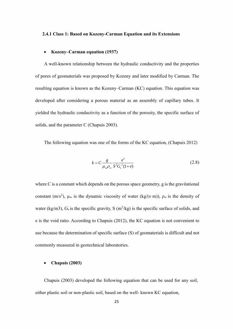
2.4.1 Class 1: Based on Kozeny-Carman Equation and its Extensions
• Kozeny–Carman equation (1937)
A well-known relationship between the hydraulic conductivity and the properties
of pores of geomaterials was proposed by Kozeny and later modified by Carman. The
resulting equation is known as the Kozeny–Carman (KC) equation. This equation was
developed after considering a porous material as an assembly of capillary tubes. It
yielded the hydraulic conductivity as a function of the porosity, the specific surface of
solids, and the parameter C (Chapuis 2003).
The following equation was one of the forms of the KC equation, (Chapuis 2012)
3
2 2 (1 )w w s
g ek C
S G e
(2.8)
where C is a constant which depends on the porous space geometry, g is the gravitational
constant (m/s2), µw is the dynamic viscosity of water (kg/(s·m)), ρw is the density of
water (kg/m3), Gs is the specific gravity, S (m2/kg) is the specific surface of solids, and
e is the void ratio. According to Chapuis (2012), the KC equation is not convenient to
use because the determination of specific surface (S) of geomaterials is difficult and not
commonly measured in geotechnical laboratories.
• Chapuis (2003)
Chapuis (2003) developed the following equation that can be used for any soil,
either plastic soil or non-plastic soil, based on the well- known KC equation,
Page 39
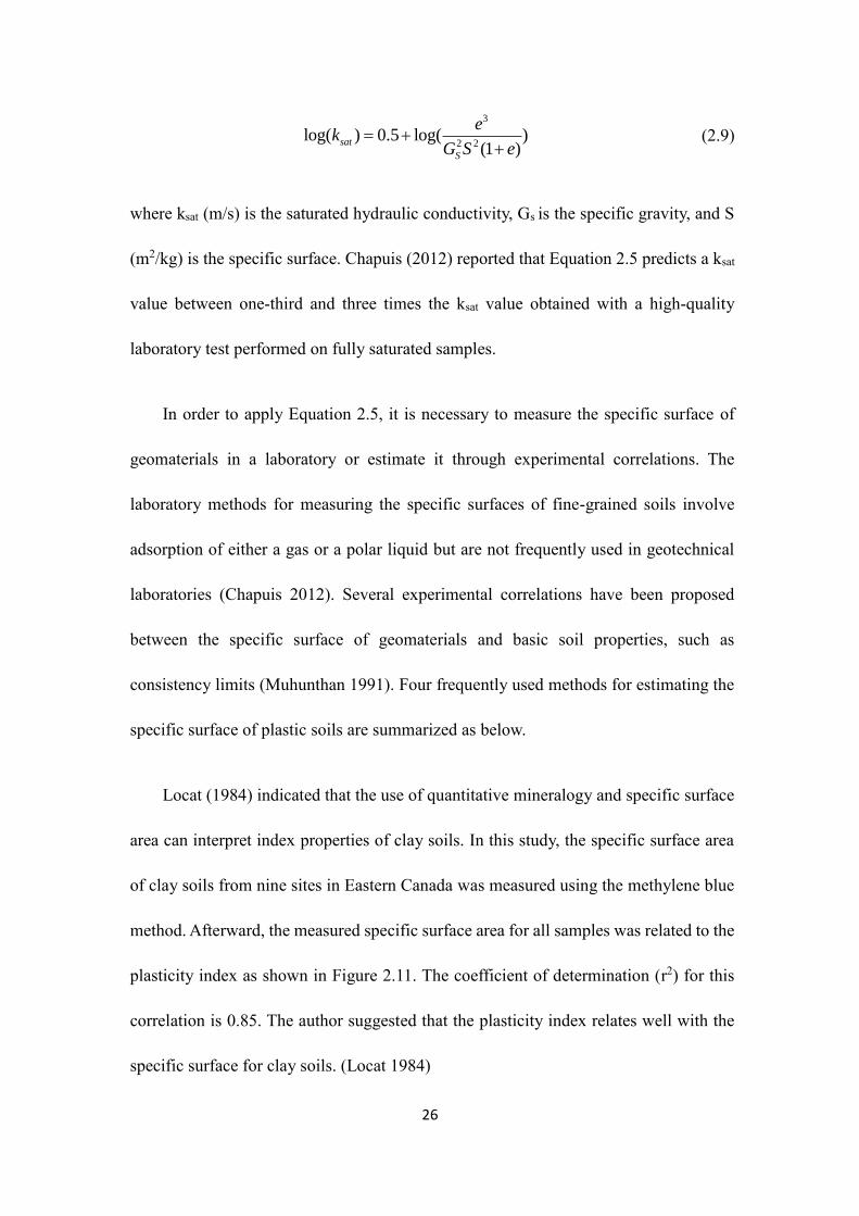
26
3
2 2log( ) 0.5 log( )
(1 )sat
S
ek
G S e
(2.9)
where ksat (m/s) is the saturated hydraulic conductivity, Gs is the specific gravity, and S
(m2/kg) is the specific surface. Chapuis (2012) reported that Equation 2.5 predicts a ksat
value between one-third and three times the ksat value obtained with a high-quality
laboratory test performed on fully saturated samples.
In order to apply Equation 2.5, it is necessary to measure the specific surface of
geomaterials in a laboratory or estimate it through experimental correlations. The
laboratory methods for measuring the specific surfaces of fine-grained soils involve
adsorption of either a gas or a polar liquid but are not frequently used in geotechnical
laboratories (Chapuis 2012). Several experimental correlations have been proposed
between the specific surface of geomaterials and basic soil properties, such as
consistency limits (Muhunthan 1991). Four frequently used methods for estimating the
specific surface of plastic soils are summarized as below.
Locat (1984) indicated that the use of quantitative mineralogy and specific surface
area can interpret index properties of clay soils. In this study, the specific surface area
of clay soils from nine sites in Eastern Canada was measured using the methylene blue
method. Afterward, the measured specific surface area for all samples was related to the
plasticity index as shown in Figure 2.11. The coefficient of determination (r2) for this
correlation is 0.85. The author suggested that the plasticity index relates well with the
specific surface for clay soils. (Locat 1984)
Page 40
27
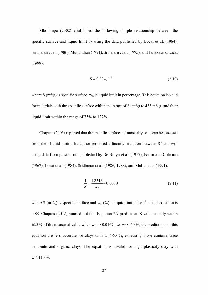
Mbonimpa (2002) established the following simple relationship between the
specific surface and liquid limit by using the data published by Locat et al. (1984),
Sridharan et al. (1986), Muhunthan (1991), Sitharam et al. (1995), and Tanaka and Locat
(1999),
1.450.20 LS w (2.10)
where S (m2/g) is specific surface, wL is liquid limit in percentage. This equation is valid
for materials with the specific surface within the range of 21 m2/g to 433 m2/ g, and their
liquid limit within the range of 25% to 127%.
Chapuis (2003) reported that the specific surfaces of most clay soils can be assessed
from their liquid limit. The author proposed a linear correlation between S-1 and wL-1
using data from plastic soils published by De Bruyn et al. (1957), Farrar and Coleman
(1967), Locat et al. (1984), Sridharan et al. (1986, 1988), and Muhunthan (1991).
1 1.3513
0.0089w LS
(2.11)
where S (m2/g) is specific surface and wL (%) is liquid limit. The r2 of this equation is
0.88. Chapuis (2012) pointed out that Equation 2.7 predicts an S value usually within
±25 % of the measured value when wL-1> 0.0167, i.e. wL < 60 %; the predictions of this
equation are less accurate for clays with wL >60 %, especially those contains trace
bentonite and organic clays. The equation is invalid for high plasticity clay with
wL>110 %.
Page 41
28
Dolinar (2009) proposed that the specific surface of non-swelling clay soil can be
expressed in the following equations from the Atterberg limits or the plasticity index,
and the weight portion of clay minerals in the soil,
S= (wL - 31.91p) / 0.81 (2.12)
S= (wp - 23.1p) / 0.27 (2.13)
S= (IP - 8.74p) / 0.54 (2.14)
where S (m2/g) is specific surface, wL (%), wp (%) and IP (%) are the liquid limit, plastic
limit and plasticity index, respectively. The equations (Equations 2.8, 2.9 and 2.10) are
only valid for inorganic soils at an ambient temperature of 20 °C.
• Mbonimpa (2002)
Mbonimpa (2002) proposed a set of simple equations, based on pedologic material
properties, to predict the hydraulic conductivity for granular and plastic soils., as an
extension of the KC equation. The author suggested that the fundamental equation for
hydraulic conductivity, k, can be formulated by combining the different influence factors
as follows:
k= ff fvfs (2.15)
where ff (L-1T-1) represents the function of pore fluid properties, fv (L
3L-3) represents the
function of the void space, and fs (L2) represents the function of the solid grain surface
characteristics. Then, using the experimental results taken from his study and from the
Page 42
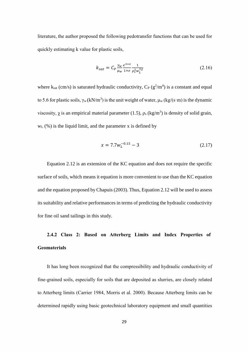
29
literature, the author proposed the following pedotransfer functions that can be used for
quickly estimating k value for plastic soils,
𝑘𝑠𝑎𝑡 = 𝐶𝑃𝛾𝑤
𝜇𝑤
𝑒3+𝑥
1+𝑒
1
𝜌𝑠2𝑤𝐿
2𝜒 (2.16)
where ksat (cm/s) is saturated hydraulic conductivity, CP (g2/m4) is a constant and equal
to 5.6 for plastic soils, γw (kN/m3) is the unit weight of water, μw (kg/(s·m) is the dynamic
viscosity, χ is an empirical material parameter (1.5), ρs (kg/m3) is density of solid grain,
wL (%) is the liquid limit, and the parameter x is defined by
𝑥 = 7.7𝑤𝐿−0.15 − 3 (2.17)
Equation 2.12 is an extension of the KC equation and does not require the specific
surface of soils, which means it equation is more convenient to use than the KC equation
and the equation proposed by Chapuis (2003). Thus, Equation 2.12 will be used to assess
its suitability and relative performances in terms of predicting the hydraulic conductivity
for fine oil sand tailings in this study.
2.4.2 Class 2: Based on Atterberg Limits and Index Properties of
Geomaterials
It has long been recognized that the compressibility and hydraulic conductivity of
fine-grained soils, especially for soils that are deposited as slurries, are closely related
to Atterberg limits (Carrier 1984, Morris et al. 2000). Because Atterberg limits can be
determined rapidly using basic geotechnical laboratory equipment and small quantities
Page 43
30
of samples, it would be very convenient to use Atterberg limits to predict the hydraulic
conductivity of geomaterials. In this section, empirical equations based on Atterberg
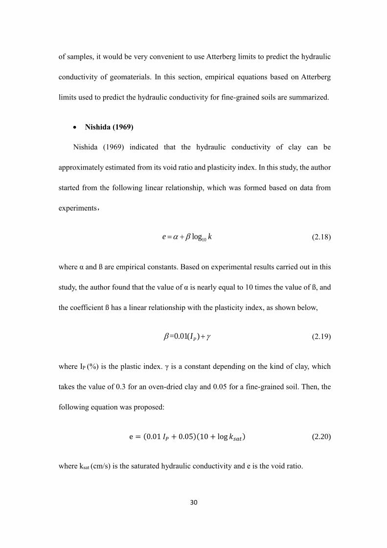
limits used to predict the hydraulic conductivity for fine-grained soils are summarized.
• Nishida (1969)
Nishida (1969) indicated that the hydraulic conductivity of clay can be
approximately estimated from its void ratio and plasticity index. In this study, the author
started from the following linear relationship, which was formed based on data from
experiments,
10loge k (2.18)
where α and ß are empirical constants. Based on experimental results carried out in this
study, the author found that the value of α is nearly equal to 10 times the value of ß, and
the coefficient ß has a linear relationship with the plasticity index, as shown below,
=0.01( )PI (2.19)
where IP (%) is the plastic index. γ is a constant depending on the kind of clay, which
takes the value of 0.3 for an oven-dried clay and 0.05 for a fine-grained soil. Then, the
following equation was proposed:
e = (0.01 𝐼𝑃 + 0.05)(10 + log 𝑘𝑠𝑎𝑡) (2.20)
where ksat (cm/s) is the saturated hydraulic conductivity and e is the void ratio.
Page 44
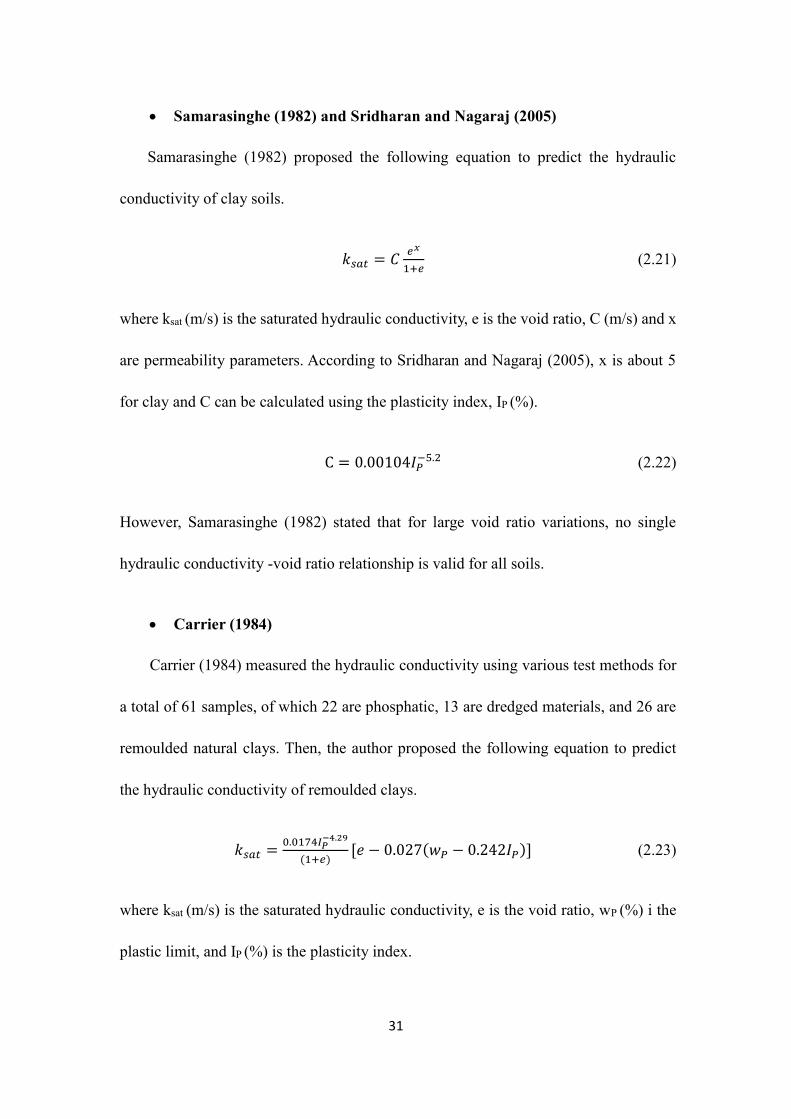
31
• Samarasinghe (1982) and Sridharan and Nagaraj (2005)
Samarasinghe (1982) proposed the following equation to predict the hydraulic
conductivity of clay soils.
𝑘𝑠𝑎𝑡 = 𝐶𝑒𝑥
1+𝑒 (2.21)
where ksat (m/s) is the saturated hydraulic conductivity, e is the void ratio, C (m/s) and x
are permeability parameters. According to Sridharan and Nagaraj (2005), x is about 5
for clay and C can be calculated using the plasticity index, IP (%).
C = 0.00104𝐼𝑃−5.2 (2.22)
However, Samarasinghe (1982) stated that for large void ratio variations, no single
hydraulic conductivity -void ratio relationship is valid for all soils.
• Carrier (1984)
Carrier (1984) measured the hydraulic conductivity using various test methods for
a total of 61 samples, of which 22 are phosphatic, 13 are dredged materials, and 26 are
remoulded natural clays. Then, the author proposed the following equation to predict
the hydraulic conductivity of remoulded clays.
𝑘𝑠𝑎𝑡 =0.0174𝐼𝑃
−4.29
(1+𝑒)[𝑒 − 0.027(𝑤𝑃 − 0.242𝐼𝑃)] (2.23)
where ksat (m/s) is the saturated hydraulic conductivity, e is the void ratio, wP (%) i the
plastic limit, and IP (%) is the plasticity index.
Page 45
32
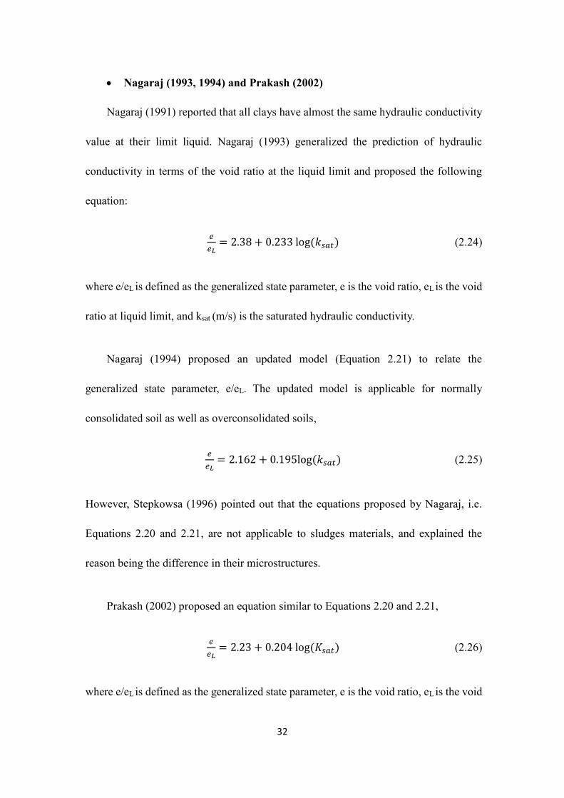
• Nagaraj (1993, 1994) and Prakash (2002)
Nagaraj (1991) reported that all clays have almost the same hydraulic conductivity
value at their limit liquid. Nagaraj (1993) generalized the prediction of hydraulic
conductivity in terms of the void ratio at the liquid limit and proposed the following
equation:
𝑒
𝑒𝐿= 2.38 + 0.233 log (𝑘𝑠𝑎𝑡) (2.24)
where e/eL is defined as the generalized state parameter, e is the void ratio, eL is the void
ratio at liquid limit, and ksat (m/s) is the saturated hydraulic conductivity.
Nagaraj (1994) proposed an updated model (Equation 2.21) to relate the
generalized state parameter, e/eL. The updated model is applicable for normally
consolidated soil as well as overconsolidated soils,
𝑒
𝑒𝐿= 2.162 + 0.195log (𝑘𝑠𝑎𝑡) (2.25)
However, Stepkowsa (1996) pointed out that the equations proposed by Nagaraj, i.e.
Equations 2.20 and 2.21, are not applicable to sludges materials, and explained the
reason being the difference in their microstructures.
Prakash (2002) proposed an equation similar to Equations 2.20 and 2.21,
𝑒
𝑒𝐿= 2.23 + 0.204 log (𝐾𝑠𝑎𝑡) (2.26)
where e/eL is defined as the generalized state parameter, e is the void ratio, eL is the void
Page 46
33
ratio at liquid limit, and ksat (m/s) is the saturated hydraulic conductivity.
Equations 2.20, 2.21 and 2.22 imply that at the liquid limit, i.e. e/eL=1, the ksat value
takes a constant value whatever the clay.
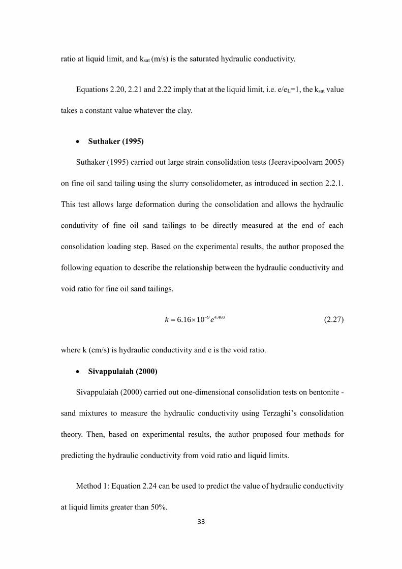
• Suthaker (1995)
Suthaker (1995) carried out large strain consolidation tests (Jeeravipoolvarn 2005)
on fine oil sand tailing using the slurry consolidometer, as introduced in section 2.2.1.
This test allows large deformation during the consolidation and allows the hydraulic
condutivity of fine oil sand tailings to be directly measured at the end of each
consolidation loading step. Based on the experimental results, the author proposed the
following equation to describe the relationship between the hydraulic conductivity and
void ratio for fine oil sand tailings.
9 4.4686.16 10k e (2.27)
where k (cm/s) is hydraulic conductivity and e is the void ratio.
• Sivappulaiah (2000)
Sivappulaiah (2000) carried out one-dimensional consolidation tests on bentonite -
sand mixtures to measure the hydraulic conductivity using Terzaghi’s consolidation
theory. Then, based on experimental results, the author proposed four methods for
predicting the hydraulic conductivity from void ratio and liquid limits.
Method 1: Equation 2.24 can be used to predict the value of hydraulic conductivity
at liquid limits greater than 50%.
Page 47
34
0.846
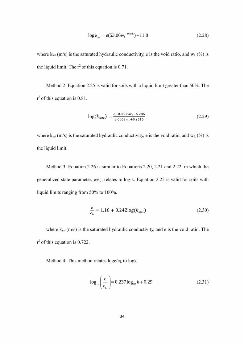
satlog (53.06 ) 11.8Lk e w (2.28)
where ksat (m/s) is the saturated hydraulic conductivity, e is the void ratio, and wL (%) is
the liquid limit. The r2 of this equation is 0.71.
Method 2: Equation 2.25 is valid for soils with a liquid limit greater than 50%. The
r2 of this equation is 0.81.
log(𝑘𝑠𝑎𝑡) =𝑒−0.0535𝑤𝐿−5.286
0.0063𝑤𝐿+0.2516 (2.29)
where ksat (m/s) is the saturated hydraulic conductivity, e is the void ratio, and wL (%) is
the liquid limit.
Method 3: Equation 2.26 is similar to Equations 2.20, 2.21 and 2.22, in which the
generalized state parameter, e/eL, relates to log k. Equation 2.25 is valid for soils with
liquid limits ranging from 50% to 100%.
𝑒
𝑒𝐿= 1.16 + 0.242log (𝑘𝑠𝑎𝑡) (2.30)
where ksat (m/s) is the saturated hydraulic conductivity, and e is the void ratio. The
r2 of this equation is 0.722.
Method 4: This method relates loge/eL to logk.
10 10log 0.237log 0.29L
ek
e
(2.31)
Page 48
35
where k (m/s) is the hydraulic conductivity, and e is the void ratio. The r2 of this
equation is 0.74. The author suggested that Method 2 is preferred compared to the other
three methods because it gives a higher correlation coefficient.
Morris et al. (2000, 2003)
Morris et al. (2000) proposed Equation 2.28 based on the index properties of mine
tailings to estimate the hydraulic conductivity. Equation 2.28 was developed based on
data from New South Wales and Queensland coal tailings, Western Australian bauxite
tailings, and Florida phosphate tailings. These data were obtained through a variety of
test methods and consist mostly of laboratory data, and field data for bauxite tailings.
𝑒
𝑒𝐿= 29.80[𝑘𝑠𝑎𝑡(1 + 𝑒)]0.177 − 0.09527 (2.32)
where ksat (m/s) is the saturated hydraulic conductivity, e is the void ratio, and eL is
the void ratio at the liquid limit. The r2 of this equation is 0.8.
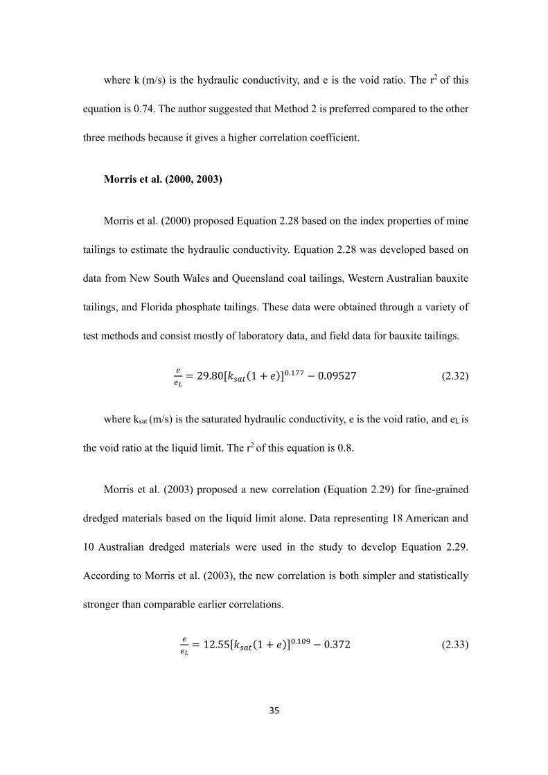
Morris et al. (2003) proposed a new correlation (Equation 2.29) for fine-grained
dredged materials based on the liquid limit alone. Data representing 18 American and
10 Australian dredged materials were used in the study to develop Equation 2.29.
According to Morris et al. (2003), the new correlation is both simpler and statistically
stronger than comparable earlier correlations.
𝑒
𝑒𝐿= 12.55[𝑘𝑠𝑎𝑡(1 + 𝑒)]0.109 − 0.372 (2.33)
Page 49
36
where ksat (m/s) is the saturated hydraulic conductivity, e is the void ratio, and eL is the
void ratio at the liquid limit. The corresponding r2 is 0.874. The authors also pointed out
that sandy (SC or SM) materials do not conform to Equation 2.29, and whether materials
with high organic contents conform to this equation is uncertain.
• Bo (2003)
Bo (2003) conducted one-step loading and step-loading compression tests for ultra-
soft soil using a Rowe cell to investigate the compression behavior in the ultra-soft stage.
Based on experimental results, the author established a correlation between the
hydraulic conductivity and void ratio under vertical and horizontal drainage conditions.
8.291
exp( )0.3155
ek
(2.34)
where k (m/s) is the hydraulic conductivity, e is the void ratio.
• Somogyi (1979) and Berilgen (2006)
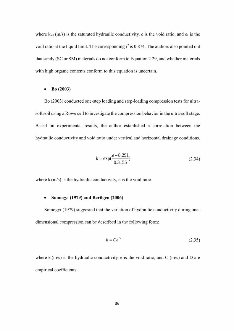
Somogyi (1979) suggested that the variation of hydraulic conductivity during one-
dimensional compression can be described in the following form:
Dk Ce (2.35)
where k (m/s) is the hydraulic conductivity, e is the void ratio, and C (m/s) and D are
empirical coefficients.
Page 50
37
Berilgen (2006) carried out seepage induced consolidation tests on clays in a slurry
consistency. The data obtained from this study, together with information already in the
literature, were used to investigate relationships between index properties and hydraulic
conductivity. The author suggested that the coefficients C and D are correlated with the
plasticity index and the liquidity index in the following forms:
C = exp[−5.51 − 4 ln(𝐼𝑃)] (2.36)
D = 7.52exp (−0.25𝐼𝐿) (2.37)
where IP (%) is plasticity index and IL (%) is liquidity index.
• Dolinar (2009)
Dolinar (2009) started from the power equation (Equation 2.31) proposed by
Somogyi (1979), and pointed out that C and D are soil-dependent parameters, which
reflect the tortuosity of the flow path and the cross-sectional characteristics of the flow
conduit, depending on the shape and the size of the particles.
In this study, the hydraulic conductivity of non-expansive clays was measured using
the falling-head test in an oedometer consolidation cell. Then, the following equations
were proposed:
6 3.03C=4.08 10 SA (2.38)
0.2342.30 SD A (2.39)
Page 51
38
0.2346 3.03 2.304.08 10 e S
Sk A (2.40)
where AS (m2/g) is the specific surface. Combining Equation 2.36 with Equation 2.10,
the following equation is proposed to predict the hydraulic conductivity of fine-grained
soils containing non-swelling clay minerals,
𝑘𝑠𝑎𝑡 =6.31∙10−7
(𝐼𝑃−8.74𝑝)3.03𝑒2.66(𝐼𝑃−8.74𝑝)
0.234
(2.41)
where ksat (m/s) is the hydraulic conductivity, e is the void ratio, IP (%) is plasticity index,
and p is the portion of clay minerals (0 ≤ p ≤ 1).
2.5 Summary
In this chapter, direct and indirect methods, as well as experimental apparatuses
used for measuring the hydraulic conductivity of geomaterials are reviewed in detail. It
is concluded that the constant head test performed in the Rowe cell is well suited for
measuring the hydraulic conductivity of soft fine-grained geomaterials over a wide
range of void ratios, hence it is adopted in this study to measure the hydraulic
conductivity of MFT. A hydraulic conductivity database of oil sand tailings is
established, which provides useful information for future studies in terms of the
investigation of consolidation behaviors of oil sand tailings. Empirical equations
developed in the literature to predict the hydraulic conductivity of fine-grained soils are
summarized. These equations are classified into two categories, i.e. Class 1, Kozeny-
Carman Equation and its Extensions; and Class 2, Equations based on Atterberg Limit
Properties.
Page 52
39
Figure 2. 1 Constant head test in the constant head permeameter
with downward flow (Head 1982)
Figure 2. 2 Mariotte bottle (Olson et. al. 1981)
Page 53
40
Figure 2. 3 Constant head test in oedometer cell (modified from Head 1982)
Figure 2. 4 Slurry consolidometer (Suthaker 1995)
Page 55
42
(c)
Figure 2. 5 (a) The large strain consolidation apparatus (b) The de-airing cylinder
(c) The tailings placement technique. (Qiu 2001)
Page 56
43
Figure 2. 6 The schematic diagram of a typical Rowe cell (modified form Head 1986)
Figure 2. 7 Falling Head Permeameter (Das, 2013)
Page 57
44
Figure 2. 8 Falling head test in oedometer consolidation cell (Owolagba 2013)
Figure 2. 9 Flow pump test (Fernandez, 1991)
Page 58
45
Figure 2. 10 Hydraulic conductivity database of oil sand tailings
Figure 2. 11 Specific surface versus plasticity index for clay soils (Locat 1984)
1.E-12
1.E-11
1.E-10
1.E-09
1.E-08
1.E-07
1.E-06
1.E-05
1.E-04
0 1 2 3 4 5 6 7 8 9 10 11
k (m
/s)
Void Ratio
Suthaker (1995) Qiu (2001) Jeeravipoolvarn et al. (2010) Miller et al. (2010)Owolagba (2013)
Page 59
46
CHAPTER 3 METHODOLOGY OF HYDRAULIC
CONDUCTIVITY MEASUREMENT OF FINE OIL SAND
TAILINGS
3.1 Introduction
Establishing the relationship between a relatively large range of void ratios and
hydraulic conductivity for fine oil sand tailings is one of the objectives of this study. As
discussed in Chapter 2, the hydraulic conductivity of soils can be determined either
indirectly and measured directly in the laboratory (Suthaker 1995). However, the
characteristics of the fine oil sand tailings posts restrictions on the test methods that
could be chosen. The measurement of hydraulic conductivity for fine oil sand tailings
and other soft fine-grained geomaterials, which have high water content and generally
in the form of slurries, is particularly challenging because these geomaterials have a
large void ratio, high compressibility, low permeability, which result in nonlinear and
lengthy consolidation.
The oedometer test, which is the standard test for measuring the consolidation
characteristics of natural soils, was adopted in this study as an indirect method to
estimate the hydraulic conductivity of fine oil sand tailings at relatively low water
content and void ratio. As discussed in Chapter 2, direct measurement methods perform
better than indirect methods for fine grained soils, particularly on soils with water
contents above the liquid limits. Two direct measurement methods were adopted in this
study, i.e., the falling head test and the Rowe cell test. The falling head test has been
widely used in geotechnical laboratories for direct measurement of the hydraulic
Page 60
47
conductivity of fine grained soils owing to its simplicity and availability of equipment
at a reasonable cost (Aiban and Znidarcic 1989, Suthaker 1995). This test was used to
measure the hydraulic conductivity of fine oil sand tailings at relatively high water
content and void ratio. The Rowe cell has many advantages, as discussed in Chapter 2.
It allows large deformations in the consolidation stage and allows the hydraulic
conductivity measurement of the sample at the end of primary consolidation of each
loading increment. The results obtained from the Rowe cell test are used to compare
with results obtained from the oedometer test and falling head test.
In this chapter, the characterization of fine oil sand tailings used in this study is
presented. Then three laboratory test methods of measuring the hydraulic conductivity
of mature fine oil sand tailings are described in detail, including the experimental
apparatus, testing procedures, and data analysis methods of the test results. The
challenges associated with the sample preparation, the test set up and execution; as well
as limitations and possible sources of errors are discussed at the end of each laboratory
test method section.
3.2 Properties of fine oil sand tailings
The samples used in this study are the mature fine oil sand tailings (MFT)
recovered from the tailings pond in Fort McMurray, Alberta, Canada, courtesy of
Syncrude Canada Ltd. and Imperial Oil Canada. The properties of mature fine tailings
are listed in Table 3.1. The specific gravity (Gs) is 2.51, and the liquid limit and plastic
limit of mature fine tailings (MFT) are 51.6% and 29.1%, respectively. The plastic
index, considered a measure of plasticity of geomaterials, is 22.5. The organic matter,
Page 61
48
which is mainly attributed to residual bitumen in MFT, is 14.7wt%. Based on the
Unified Soil Classification System (USCS), the mature fine tailings is classified as a
silt with high plasticity (MH). The mature fine oil sand tailings have high water contents
and large void ratios in tailings ponds. The natural water content is 171.3% when the
mature fine tailings (MFT) samples were received (Guo 2012).
3.3 Standard Oedometer Test
The oedometer test, also known as the one-dimensional consolidation test, is used
to determine the consolidation parameters for soils. The hydraulic conductivity of soils
can also be derived from the test results. In the standard oedometer test (ASTM D2435),
the soil sample is confined laterally and drained vertically while it is subjected to a
sequence of incremental vertical loads; and each load increment is maintained until the
excess pore water pressure is essentially dissipated.
Two standard oedometer tests (Oedo-1and Oedo-2) were carried out, and the initial
water content and void ratio of both test samples were approximately 65% and 1.6,
respectively. The next sections introduce the experimental apparatus used in the tests,
the testing procedures, and data analysis methods for the standard oedometer test.
3.3.1 Experimental Apparatus
The consolidation test unit, consisting of a fixed ring consolidometer and a loading
device, was used in this test. The test sample was confined in a stainless-steel
consolidation ring of 15.2 mm in height and 49.7 mm in diameter. A linear displacement
transducer mounted to the arm on the support post of the loading frame, as shown in
Figure 3.1, was used to measure the deformation of the test sample during the
Page 62
49
consolidation process. The linear displacement transducer and the readout unit were
manufactured from Schaevitz Equipment LTD.
3.3.2 Testing Procedures
The standard oedometer tests were performed according to ASTM D2435-11, the
standard test method for one-dimensional consolidation properties of soils using
incremental loading (ASTM D2345). The test samples were first preconsolidated in the
permeameter chamber by applying various loads on the sample and opening the
drainage port at the bottom rim of the permeameter, as shown in Figure 3.2, in order to
reach a lower water content. The preconsolidation pressure was less than the first
loading increment in the subsequence oedometer test. The test sample was
preconsolidated in the permeameter until it could sustain at least 2 kPa axial pressure.
After completing preconsolidation, the sample was trimmed to the consolidation ring.
It should be noted that the maximum water content of mature fine tailings sample used
in the oedometer test is approximately 65%, which was ascertained by trial. At water
contents higher than 65%, corresponding to a void ratio of 1.6, the oedometer test may
not be suitable for the hydraulic conductivity measurement because the too soft sample
can not be properly trimmed to a consolidation ring. In addition, very large nonlinear
deformation can occur during consolidation for a soft sample, which results in errors in
the back-calculation based on Terzaghi’s one dimensional consolidation theory.
A standard incremental load was applied to two standard oedometer tests (Oedo-
1and Oedo-2) in the following sequence: 5kPa, 10kPa, 25 kPa, 50 kPa, 100 kPa, 200
kPa and 400 kPa. The displacement readout was recorded and collected at 16 time
Page 63
50
intervals: 6s, 15s, 30s, 1min, 2min, 4min, 8min, 15min, 30min, 1h, 2h, 4h, 6h, 24h, 48
and 72h. The sample deflection versus time was recorded during the test to monitor the
progress of primary consolidation and to decide the time to apply to the next load
increment. For MFT samples used in oedometer tests, the loading increment of 72 hours
was proved to be reasonable.
3.3.3 Data Analysis
To back calculate the hydraulic conductivity from consolidation parameters, the
coefficient of consolidation and the coefficient of volume change are assumed constant
over each loading increment, and using the following equation that is derived from
Terzaghi's one-dimensional consolidation theory (Budhu 2008),
z w v vk c m (3.1)
where, kz (L/T) is the hydraulic conductivity in the vertical direction, γw (M/T2L3) is the
unit weight of water (9.8 kN/m3), Cv (L2/T) is the coefficient of consolidation, which is
determined from two commonly used curve fitting methods, i.e. Cassagrande’s
logarithmic time method and Taylor’s square root time method (Gofar and Kassim
2006), and mv (LT2/M) is the coefficient of volume change or modulus of volume
compressibility. After obtaining the values Cv, and mv, the values of γw, Cv, and mv were
substituted to Equation 3.1. The hydraulic conductivity values of mature fine tailings
were obtained, and then the relationship between the hydraulic conductivity and void
ratio for the mature fine oil sand tailings was established.
3.3.4 Discussion
The standard oedometer test, as a basic laboratory test, has been widely used in
Page 64
51
geotechnical laboratories. However, based on the standard ASTM-D2435, the
oedometer test was not applicable for the slurry-like soil such as the mature fine oil
sand tailings with high water content, because of its large void ratio and high
compressibility during self-consolidation stages (Proskin et al. 2010). The standard
oedometer test was developed for the soil that is in a relatively solid phase with a shear
strength of no less than 2 kPa (Olson and Daniel 1981). The other limitation is that the
oedometer used in this study cannot measure the excess pore water pressure, therefore,
the completion of primary consolidation is based solely on the change of sample height
(Gofar and Kassim 2006).
In addition, the maximum initial water content of the MFT sample that can be used
in the standard oedometer test is approximately 65%, which was estimated by trials,
corresponding to a void ratio of 1.6. As discussed previously, at water contents higher
than 65%, two major difficulties can invalidate the oedometer test for determining the
hydraulic conductivity. For samples with higher void ratios, other measurement
methods must be adopted.
3.4 Falling Head Test
The falling head permeability test, also known as the falling head test, is one of the
most commonly used laboratory tests for the direct measurement of hydraulic
conductivity (ASTM D5856). The falling head test is usually used for fine-grained soils
with intermediate and low permeability. The mature fine tailings used in this study fits
in this category. Another method, i.e. The constant head test (ASTM D5856) is used for
coarse grained soils with high permeability. These two methods are widely used in
Page 65
52
geotechnical laboratories owing to simplicity and availability of equipment at a
reasonable cost (Aiban and Znidarcic 1989, Suthaker 1995).
The falling head tests with the downward flow and constant tail water elevation
were carried out in this study on MFT samples of a wide range of void ratios, from
approximately 1.5 to 7.0. A detailed description of the falling head test is given in
ASTM D5856 Standard Test Method for Measurement of Hydraulic Conductivity of
Porous Material Using a Rigid-Wall, Compaction-Mold Permeameter (ASTM D5856).
3.4.1 Experimental Apparatus
A rigid wall permeameter from Hoskin Scientific LTD. and an open standpipe fitted
with a meter stick were used in this test. The permeameter chamber with 150 mm in
height and 76.3 mm in inner diameter was used to place the sample. This permeameter
allows for observation of the sample height from the transparent plexiglass wall. Water
flowing through MFT samples from the standpipe connected to the influent port at the
top plate of the permeameter and then to the funnel which was connected to the drainage
port at the bottom rim of the permeameter, as the schematic diagram shown in Figure
3.3. This arrangement allows the downward hydraulic gradient to be applied to the test
sample. The standpipe and funnel were connected to the permeameter both by rubber
tubes. The funnel was clamped to the meter stick and used to maintain a constant
tailwater level. The realistic view of the arrangement of the falling head test with the
downward flow is shown in Figure 3.4.
3.4.2 Testing Procedures
The falling head tests were performed according to ASTM D5856 Standard Test
Page 66
53
Method for Measurement of Hydraulic Conductivity of Porous Material Using a Rigid-
Wall, Compaction-Mold Permeameter, Method B - Falling head, constant tailwater
elevation (ASTM D5856). The sample with the natural water content of 171.3% was
first preconsolidated in the permeameter chamber to reach a predetermined water
content for the falling head tests by applying incremental vertical loads on the top of
the sample and opening the drainage port of the permeameter, as shown in Figure 3.5.
Another method of sample preparation was that the sample was first mixed with de-
aired water and curing for 24 hours. The sample height was measured and recorded
during consolidation. The sample height versus elapsed time was recorded and was
plotted against log time, as shown in Figure 3.6. This step allows the falling head test
to be conducted under a stable void ratio of the sample.
In the falling head test, the following values were recorded: the initial and final
heads, denoted by h1 and h2, respectively (shown in Figure 3.3); the time t
corresponding to h1 to h2; and the temperature, T, of the tail water in the funnel. The
height of the sample was measured and recorded at the start and end of each permeation
trial. Four or five permeation trials were conducted consecutively to obtain at least four
values of hydraulic conductivity in one falling head test. At the end of the test, the
permeameter was dismantled and the final water content of the test sample was
determined.
3.4.3 Data Analysis
The hydraulic conductivity is calculated from the falling head test by using the
following equation (Holtz and Kovacs, 1981):
Page 67
54
av 110
2
2.303 logT
aL hk
At h (cm/s) (3.2)
where kT (cm/s) is the hydraulic conductivity in the vertical direction carried out at T◦C,
a (cm2) is the cross-sectional area of the standpipe, Lav (cm) is the average value of the
sample height at the beginning and end of each permeation trial. A (cm2) is the cross-
sectional area of the test sample, h1 (cm) and h2 (cm) are initial and final hydraulic head
difference, respectively, t (s) is the time duration for the head difference dropping from
h1 to h2. Then the kT value was corrected to a baseline temperature of 20◦C by using the
following equation (Budhu 2007):
20
20
( )=TT T Tk k k R
(3.3)
where µT and µ20 are the viscosities of water at T◦C and 20◦C, respectively. T is the
temperature at which the permeation trial was made, and RT is the temperature
correction factor that was calculated using the following equation:
2.42 0.475ln( )TR T (3.4)
After calculating the average value of hydraulic conductivity, k20, which was obtained
from each permeation trial in one falling head test, the relationship of the test sample
between the hydraulic conductivity and void ratio was obtained.
3.4.4 Discussions
The falling head test has been widely used in geotechnical laboratories owing to its
simplicity and the availability of equipment at a reasonable cost (Suthaker 1995), as
well as the simplicity of interpretation of test data.
For the soil sample with low permeability, it is usually necessary to apply larger
Page 68
55
hydraulic gradients in the laboratory to accelerate the test, while a high hydraulic
gradient produces high seepage force that can consolidate soft and compressible
samples, which results in reducing the sample hydraulic conductivity as the test
proceeds. Therefore, the major challenge for the falling head test was applying an
appropriate hydraulic gradient to the samples without causing significant consolidation
and to avoid prolonged testing time. The sample height should be continuously
monitored during the test. Once an obvious change of the sample height occurs the test
should be terminated.
Due to limitations of the experimental conditions, two possible sources of errors
for this test are identified: 1) The test can only measure the inflow rate, which may lead
to an error in obtaining the hydraulic conductivity value, especially for soft fine-grained
soils in which consolidation and permeability may occur together (Chapuis 2012); 2)
Evaporation from the standpipe or the tail water funnel may occur, which would lead
to overestimation of the hydraulic conductivity values.
In addition, the minimum water content of the MFT samples that can be achieved
by consolidating the sample in the permeameter is approximately 60%. Therefore, in
this study, the falling head test can measure the hydraulic conductivity of MFT samples
with water contents higher than 60%, corresponding to a void ratio of 1.5.
3.5 Rowe Cell Test
The Rowe cell, also known as the hydraulic consolidation cell, was developed by
P. W. Rowe and his research group to overcome the disadvantages of the conventional
oedometer apparatus when performing consolidation tests on low permeability soils
Page 69
56
(Head 1986). A detailed description of the experimental apparatus and ancillary devices,
testing procedures, and data analysis methods for the Rowe cell test are presented in
this section.
The schematic diagram of a typical Rowe cell is shown in Figure 3.7 (a). The main
feature of the Rowe cell is its hydraulic loading system. In the Rowe cell, a sample is
loaded hydraulically by water pressure acting on a convoluted flexible diaphragm,
which differs from the mechanical lever system used in the conventional oedometer.
This allows for testing large diameter samples, i.e, up to 250 mm diameter for
commercial purposes, and allows for large deformations in consolidation. With the
hydraulic loading system, the loading pressure, including very low pressures, can be
easily applied (Head 1986). In contrast to the conventional oedometer apparatus, the
Rowe cell allows the direct measurement of hydraulic conductivity, either as an
independent test or after the consolidation test on a sample with a known vertical
effective stress. More importantly, the Rowe cell has abilities to control drainage
conditions, to measure pore water pressure during the consolidation stage, and to apply
back pressure throughout the test, as introduced in Chapter 2.
In this study, four Rowe cell tests, i.e. RC 1, RC 2, RC 3 and RC 4, were carried
out to measure the hydraulic conductivity of MFT over a wide range of void ratios,
from approximately 1 to 6. This range partially overlaps with the ranges of the standard
oedometer test and falling head test. Each Rowe cell test includes step loadings
consolidation tests and permeability tests. A permeability test was performed during the
consolidation test sequence at the end of each loading stage.
Page 70
57
3.5.1 Experimental Apparatus
The following apparatuses were used in this study for Rowe cell tests:
• A Rowe cell
• A Brainard. Kilman pressure control panel (B.K panel)
• A vertical pressure transducer
• A pore water pressure transducer
• A linear displacement transducer
• A volume change indicator
• A data logger
A Rowe cell produced by ELE International, UK, of 150 mm nominal diameter was
used in this study, as shown in Figure 3.7 (b). The cell has an internal diameter of 150.4
mm with a smooth plastic lining, as shown in Figure 3.8 (b). The cell consists of three
parts: the cell top, the cell body, and the cell base, as shown in Figure 3.8. The cell top
is fitted with a convoluted flexible diaphragm made of synthetic rubber, which is used
to transmit a uniform water pressure to the sample underneath. The cell top is also fitted
with an inlet valve, denoted by valve C as shown in Figure 3.7 (a), connecting to a
hydraulic pressure on a sample. An aluminum alloy hollow spindle passes through a
seal in the center of the cell top. The lower end of this spindle passes through the center
of the diaphragm at which it is sealed and fixed by two thin washers. The upper end of
it is connected to a drainage valve, denoted by valve D, via a flexible tube, as shown in
Figure 3.7 (a). The drainage valve D is fitted to the edge of the cell top. An air bleed
screw, denoted by E as shown in Figure 3.7 (a), is placed on the top of the cell top. The
Page 71
58
cell body has a flange at each end with bolt holes for securing the cell top and base, as
shown in Figure 3.8 (b). A small hole at the upper end of the cell body is an outlet
leading and connected to a valve, denoted by valve F as shown in Figure 3.7 (a). A
smooth plastic lining is bonded onto the inside face of the cell body to reduce the
friction between the sample and cell wall. A small circular pore stone is inserted in the
center of the cell base. This is the main pore water pressure measuring point, and leads
to valve A (as shown in Figure 3.7 (a)) on the outer edge of the cell base. Valve A is
connected to the pore water pressure transducer. (Head 1986)
Two large pore stones obtained from Hoskin Scientific LTD of 150 mm in diameter
and 13 mm in thickness are used with the Rowe cell, as shown in Figure 3.9.
A Brainard-Kilman pressure control panel (B.K panel) is used to provide three
independently controlled pressures required for the Rowe cell test: the vertical pressure,
and two separate back pressures. The realistic view and schematic diagram of the B.K
panel are shown in Figures 3.10 and 3.11, respectively. The three pressure systems are
fitted on the B.K panel on positons 1, 2 and 3, respectively, as shown in Figure 3.11.
The B.K pressure control panel has an accuracy of 1kPa (B.K. panel operation manual).
The vertical pressure transducer, which has a better accuracy of 0.1 kPa compared
with the B.K pressure control panel, measured the real-time pressure applied on the
sample. The pore water pressure was measured by the pore water pressure transducer,
which has an accuracy of 0.1 kPa. A linear displacement transducer was used to measure
vertical displacements of the sample during the test. It has a maximum travel of 25 mm
and has the accuracy of 0.001 mm. The above transducers were manufactured by
Page 72
59
Dynisco Ltd.
The volume change indicator (SHAPE Instrument Ltd.), as shown in Figure 3.12,
was used to measure the volume of the outflow water during the consolidation test and
permeability test. It was incorporated into the drainage line of the Rowe cell test
arrangement by connecting with valve D. The volume change indicator used in this
study has the maximum capacity of 100ml and has the accuracy 0.01ml. All the
measured data, including vertical pressure, pore water pressure, deflections of the
testing sample and the volume of the outflowing water, were recorded by the data logger
(SCIEMETRIC INC).
3.5.2 Testing Procedures
For the MFT samples having a water content much higher than the liquid limit, it
is necessary to start with applying a low consolidation pressure and gradually increase
in a few increments. In this study, four Rowe cell tests were performed.
In the first Rowe cell test (RC 1), the sample with an initial water content of 176.9%
was consolidated under four loading increments with a back pressure. The incremental
vertical loading was applied in the following sequence: 7 kPa, 12 kPa, 17 kPa and 43
kPa. The corresponding back pressure for each loading step was applied in the
following sequence: 5 kPa, 7 kPa, 10 kPa and 33 kPa. Thus, the theoretical effective
stresses of the sample after the completion of each loading consolidation were as
follows: 2 kPa, 5 kPa, 7 kPa and 10 kPa. The above pressures applied in the RC 1 test
are summarized in Table 3.2. After the completion of primary consolidation under each
loading, one-way drainage permeability tests were carried out on the samples of known
Page 73
60
effective stress in the Rowe cell with the vertical upward flow. Two constant back
pressures were applied to the sample to provide a constant differential pressure between
the sample base and top, while the sample was subjected to a vertical pressure as in the
previous consolidation step. The differential pressures applied to the sample at each
permeability test are also summarized in Table 3.2.
In the second Rowe cell test (RC 2), the sample with an initial water content of
129.7% was consolidated by incremental loading. A back pressure of 10 kPa was
maintained during the test. The incremental vertical loads were: 12 kPa, 13 kPa, and 15
kPa. Thus, the theoretical effective stresses on the sample after the completion of
consolidation in each stage were: 2 kPa, 3 kPa, and 5 kPa. At the end of each
consolidation stage, the permeability test was carried out under a constant differential
pressure. Pressures applied in the RC 2 test are summarized in Table 3.3.
In the third Rowe cell test (RC 3), the sample with an initial water content of 210.4%
was consolidated under four loading increments with a back pressure of 5 kPa. The
incremental vertical loads were: 7 kPa, 8 kPa, 9 kPa and 10 kPa. The theoretical
effective stresses on the sample after the completion of consolidation in each stage were:
2 kPa, 3 kPa, 4 kPa and 5 kPa. At the end of each consolidation stage, a permeability
test was carried out under a constant differential pressure. Pressures applied in the RC
3 test are summarized in Table 3.4.
In the fourth Rowe cell test (RC 4), the sample with an initial water content of 76.7%
was consolidated in four increments with a back pressure of 10 kPa. The incremental
vertical loads were: 15 kPa, 20 kPa, 30 kPa and 50 kPa. The theoretical effective
Page 74
61
stresses on the sample after the completion of consolidation in each stage were: 5 kPa,
10 kPa, 20 kPa and 40 kPa. At the end of each consolidation stage, a permeability test
was carried out under a constant differential pressure. Pressures applied in the RC 4 test
are summarized in Table 3.5.
In this study, the Rowe cell tests were carried out primarily based on Hydraulic
Cell Consolidation and Permeability Test in the Manual of Soil Laboratory Testing
(Head 1986), while some steps were modified to accommodate the B.K pressure system.
A detailed description of the test executions is introduced in the following steps.
Step 1. Cell assembly
The cell body was first bolted to the cell base, as shown in Figure 3.13. MFT
samples were poured into the cell to a depth of 15-30 mm with a uniform surface. Then,
the cell top was placed on the cell body, and the diaphragm flange of the cell top was
seated onto the cell body flange without entrapping air or causing ruckling or pinching,
as shown in Figure 3.14. The view of the correctly seated diaphragm flange on the cell
body flange is shown in Figure 3.15. After completing the cell assembly, the valve C
(Rowe cell) was connected to a water supply to completely fill the space above the
diaphragm with water. (Head 1986)
Step 2. Rowe cell connection with B.K pressure system
The arrangement of the Rowe cell and connections with a B.K Pressure control
panel are shown in Figure 3.16. The valve C (Rowe cell) was connected with valve Q1
(B.K panel) through a flexible tube, as shown in Figure 3.18. This line provided vertical
hydraulic pressures on the sample throughout the Rowe cell test. The valve A (Rowe
Page 75
62
cell) was connected with valve Q2 (B.K panel) through a flexible tube, as shown in
Figure 3.18. This line provided one of the back pressure to the sample during
permeability test but kept closed during consolidation stage. The valve D (Rowe cell)
was connected to the volume change indicator, which was then connected to the valve
Q3 (B.K panel), as shown in Figure 3.16. This line was the drainage line in which water
flowed out of the sample through valve D (Rowe cell) to the volume change indicator;
which provides another back pressure to the sample throughout the Rowe cell test. The
above three lines were fully saturated with freshly de-aired water and de-aired by
flushing with de-aired water to ensure saturation.
Then, the vertical pressure transducer, pore water pressure transducer, displacement
transducer and volume change indicator were connected to the data-logger. The
readings showing on the data logger were calibrated to be consistent with the readings
showing on the B.K pressure panel.
Step 3. Checking Saturation
The degree of saturation of MFT samples can be related to the pore pressure ratio,
i.e. δu/δσ, where δu is the pore pressure response to an increment of the total vertical
stress δσ without drainage (Head 1986). It should be noted that this ratio is not the exact
pore pressure parameter B, which is defined as the pore pressure response to the
increments of isotropic stress not vertical stress. However, the similar method was used
to check the saturation of the sample in this study. Saturation is usually acceptable when
the ratio δu/δσ reaches approximately 0.9 (Head 1986). The detailed execution of
checking saturation degree of samples is introduced as follows.
Page 76
63
A very small vertical pressure, p0, which was less than the first increment
consolidation pressure, was applied to the sample without drainage (valve D closed).
The initial vertical pressure, p0, and the initial pore pressure, u0, were recorded by the
data logger when p0 and u0 reach a stable value. Then, the vertical pressure was
increased from the initial pressure p0 to a value that gave the required first increment
pressure p1, typically an increase of 3 to 5 kPa on the sample, without drainage. The
pore pressure u1 was recorded when it reached a stable value. The initial ratio, δu/δσ,
was calculated as:
1 0
1 0
u uu
p p
(3.5)
The initial ratios (δu/δσ) of the MFT samples used in this study were larger than 0.92,
which means the samples satisfy the test saturation requirement. After checking the
saturation condition of the sample, the vertical pressure was set back to the initial
pressure p0.
Step 4. Consolidation Test
The vertical pressure was set to the first increment consolidation pressure on the
B.K panel with valve C (Rowe cell) closed. The back pressure was set to a desired value
corresponding to the first incremental loading with valve D (Rowe cell) closed. The
data logger was first to run to record the initial vertical deflection reading and the initial
volume change indicator readings, corresponding to time equal to zero.
The consolidation stage was started by opening valves C and D to apply vertical
pressure and back pressure on the sample and allow water to be expelled from the
sample. Once opened valves C and D allowed water to drain from the sample, the
Page 77
64
applied stress was transferred from the pore water to the soil skeleton, increasing the
effective stress, while the total applied vertical stress was held constant. The following
data were recorded by the data logger at an appropriate time intervals.
• Vertical settlement
• Pore water pressure
• Volume-change indicator on outlet back pressure line
• Diaphragm pressure for checking purpose
As the consolidation stage proceeded, the following graphs were created.
• Settlement (∆H mm) against log time (min)
• Outflow volume change (∆V mm) against log time (min)
• Pore water pressure against time (min)
The permeability test was performed when the primary consolidation was
completed based on instruction listed above, i.e. the pore pressure approached the back
pressure. For most practical purposes, 95% dissipation of the excess pore pressure is
sufficient (Head 1986). The percentage pore pressure dissipation, denoted by U%, is
given by the following equation:
0
0
100%b
u uU
u u
(3.6)
where, u is the pore water pressure at a time considered, ub is the back pressure applied
in the consolidation stage, and u0 is the pore water pressure at the start of consolidation.
Step 5. Permeability test
One-way drainage permeability tests were carried out on the samples of known
effective stress in the Rowe cell with the vertically upward flow. Three independently
Page 78
65
controlled constant pressure systems were used for the permeability test. One system
was connected to valve C (Rowe cell) to maintain the pressure as applied in the previous
consolidation step. The other two back pressures were connected to valve A and D,
respectively, as shown in Figure 3.16. The arrangement of the Rowe cell for the one-
way drainage permeability test is shown in Figure 3.17, and this arrangement allows
water to vertically flow upward through the sample by applying different inlet (p2) and
outlet (p1) pressures between the sample base and top, while the sample was subjected
to a vertical pressure as the in previous consolidation step.
The differential pressure between the inlet and outlet was adjusted by trial and error
to establish a reasonable rate of flow through the sample. In this study, 1 or 2 kPa
differential pressure, ∆p, between the inlet and outlet was used (shown in Tables 3.2 to
3.5), which was ascertained from the trials. The procedure for the permeability test in
the Rowe cell is described as follows:
The outlet pressure P2 was maintained the same as the back pressure applied in the
consolidation stage. The inlet pressure P1 was adjusted by starting with a pressure equal
to P2 and increasing progressively, but this pressure must never exceed the vertical
pressure. The differential pressures ∆p applied in the permeability tests are shown in
Tables 3.2- 3.5.
The volume of the cumulative outflow water Q (ml) and the elapsed time t (s) were
recorded by the data logger. As the permeability test proceeded, the graph of the
cumulative outflow water Q (ml) on ordinate against the elapsed time t (minute) on
abscissa was plotted. The test was continued until a steady rate of flow was reached, i.e.
Page 79
66
the graph presented a linear segment. In this study, permeability tests generally lasted
1.5 to 2 hours to allow enough linear segment on the graph to emerge. The permeability
test was stopped by closing valves A and D.
Step 6. Further consolidation tests and permeability tests
Additional tests at the higher effective stress level were carried out by either raising
the vertical pressure only or by raising vertical pressure and back pressure both but with
different increments to the predetermined value. In this study, the samples were
consolidated 3 or 4 times at the subsequent loading levels by increasing the vertical
pressure and back pressure to the desired value, as summarized in Tables 3.2- 3.5.
The procedures described in Step 4--Consolidation Test were repeated. After
setting up the vertical pressure and back pressure to the next loading level on the B.K
pressure control panel, valves C and D were opened simultaneously to allow water to
be expelled from the sample under a new consolidation pressure. When the primary
consolidation was completed, the permeability test was carried out by repeating the
procedures as described in Step 5 on a sample under a new void ratio and effective
stress level.
After the samples were consolidated 3 or 4 times, the Rowe cell was disassembled
and the final water content was measured.
3.5.3 Data analysis
The hydraulic conductivity can be directly measured by the Rowe cell tests. The
graph of the cumulative outflow water Q (ml) against the elapsed time t (minute) was
plotted, in which the slope of the linear segment of the graph was used to calculate the
Page 80
67
rate of flow, q (ml/minute), i.e. q = δQ/δt (ml/minute). The pressure difference ∆p across
the soil sample was equal to (p2 – p1). The hydraulic conductivity of the sample can be
calculated by using the following equation based on Darcy’s Law, (Head 1986)
60
VV
qk
Ai (m/s) (3.7)
where kv is the hydraulic conductivity in vertical direction (m/s), qv is the rate of vertical
flow (ml/minute) obtained from the slope of the linear part of the graph of the
cumulative outflow water Q against the elapsed time t, A is the sample cross-sectional
area (mm2), approximately 18,000mm2, and i is the hydraulic gradient. A pressure
difference of 1 kPa is equivalent to a water head 1/9.81m≈102 mm (Head 1986). Thus,
the hydraulic gradient i can be calculated from the following equation:
102
i PH
(3.8)
where, ∆p (kPa) is the pressure difference between the inlet pressure p2 and outlet
pressure p1, and H is the height of the sample (mm). Substituting Equation 3.8 into
Equation 3.7, the hydraulic conductivity, kv, can be expressed as:
60 60 102 6120
V V VV
q q H q Hk
Ai A P A P
(3.9)
The hydraulic conductivity values calculated from Equation 3.9 were corrected to
the equivalent values at 20◦C by using the temperature correction factor RT, as
introduced in Section 3.4.3.
The void ratio corresponding to each hydraulic conductivity value of the sample
was back-calculated from the final void ratio after obtaining the final water content.
Page 81
68
3.5.4 Discussion
The most important feature of the Rowe cell is that it allows the consolidation and
permeability tests to be directly and successively conducted, which provides data
covering a wide range of void ratios or strains (Gofar and Kassim 2006). The Rowe cell
test can be used for the measurement of the hydraulic conductivity of the MFT samples,
partially overlapping with the ranges of the standard oedometer tests and falling head
tests. In addition, the advanced hydraulic loading system, and the abilities to control
drainage and to measure pore water pressure, as well as to apply the back pressure to
the sample, contribute to more reliable results compared to other methods.
3.6 Summary
This chapter describes in detail the experimental apparatus, testing procedures and
data analysis for the standard oedometer test, the falling head test and Rowe cell test
used in this study to measure the hydraulic conductivity of mature fine oil sand tailings.
In the standard oedometer test, the incremental loads were applied to the samples, and
vertical settlements were measured throughout the test. Due to the limitations of the
test, the ASTM-D2435 standard oedometer test was not applicable for the MFT samples
with the initial water content and void ratio higher than 65 % and 1.6, respectively.
The falling head test was chosen as one of the direct measurement methods to
determine the hydraulic conductivity of the mature fine oil sand tailings. The major
difficulty encountered during the test was adjusting an appropriate hydraulic gradient
to the MFT samples to avoid the prolonged testing time and to avoid consolidation.
Then, two possible sources of errors for this test were recognized because of limitations
Page 82
69
of the experimental conditions.
The Rowe cell test overcomes the disadvantages inherent in the standard oedometer
test and falling head test for measuring the hydraulic conductivity of the mature fine
tailings. The Rowe cell test is capable of testing the sample covering a large range of
void ratios, which partially overlaps the range of both standard oedometer and falling
head tests. Comparing three laboratory test methods, the Rowe cell test is more complex
than the other two tests in terms of the experimental apparatus assembly and connection,
as well as test execution. In addition, the advanced control features, the ability to
measure pore water pressure and the ability to apply back pressure on the sample
contribute to more reliable test results obtained with Rowe cell tests.
Page 83
70
Table 3. 1 Properties of mature fine tailings (modified from Guo 2012)
Specific gravity, Gs 2.51
Organic matter (%) 14.7
Atterberg limits Plastic limit, PL (%) 29.1
Liquid limit, LL (%) 51.6
Plasticity index, PI (%) 22.5
Grain size D10 (μm) 0.85
D50 (μm) 7.15
D90 (μm) 27.9
Sand (%) 0.00
Silt (%) 80.00
Clay (%) 20.00
Unified Soil Classification MH
Page 84
71
Table 3. 2 Summary of Rowe cell test 1 (RC 1)
Vertical
Pressure
(kPa)
Outlet Back
Pressure
P2 (kPa)
Inlet Back
Pressure
P1 (kPa)
Effective stress
after consolidation
σ’ (kPa)
Differential
Pressure ∆p
(kPa)
C-1a 7 5 n/a 2 n/a
P-1b 7 5 6 2 1
C-2 12 7 n/a 5 n/a
P-2 12 7 9 5 2
C-3 17 10 n/a 7 n/a
P-3 17 10 12 7 2
C-4 43 33 n/a 10 n/a
P-4 43 33 35 10 2
a. C refer to consolidation test;
b. P refers to permeability test
Table 3. 3 Summary of Rowe cell test 2 (RC 2)
Vertical
Pressure
(kPa)
Outlet Back
Pressure
P2 (kPa)
Inlet Back
Pressure
P1 (kPa)
Effective stress
after consolidation
σ’ (kPa)
Differential
Pressure ∆p
(kPa)
C-1a 12 10 n/a 2 n/a
P-1b 12 10 11 2 1
C-2 13 10 n/a 3 n/a
P-2 13 10 12 3 2
C-3 15 10 n/a 5 n/a
P-3 15 10 12 5 2
a. C refer to consolidation test;
b. P refers to permeability test
Page 85
72
Table 3. 4 Summary of Rowe cell test 3 (RC 3)
Vertical
Pressure
(kPa)
Outlet Back
Pressure
P2 (kPa)
Inlet Back
Pressure
P1 (kPa)
Effective stress after
consolidation σ’
(kPa)
Differential
Pressure ∆p
(kPa)
C-1a 7 5 n/a 2 n/a
P-1b 7 5 6 2 1
C-2 8 5 n/a 3 n/a
P-2 8 5 6 3 1
C-3 9 5 n/a 4 n/a
P-3 9 5 6 4 1
C-4 10 5 n/a 5 n/a
P-4 10 5 6 5 1
a. C refer to consolidation test;
b. P refers to permeability test
Table 3. 5 Summary of Rowe cell test 4 (RC 4)
Vertical
Pressure
(kPa)
Outlet Back
Pressure
P2 (kPa)
Inlet Back
Pressure
P1 (kPa)
Effective stress after
consolidation σ’
(kPa)
Differential
Pressure ∆p
(kPa)
C-1a 15 10 n/a 5 n/a
P-1b 15 10 12 5 2
C-2 20 10 n/a 10 n/a
P-2 20 10 12 10 2
C-3 30 10 n/a 20 n/a
P-3 30 10 12 20 2
C-4 50 10 n/a 40 n/a
P-4 50 10 12 40 2
a. C refer to consolidation test;
b. P refers to permeability test
Page 86
73
Figure 3. 1 The consolidation test unit
(a) (b)
Figure 3. 2 Preconsolidation of sample in permeameter before the oedometer test
Page 87
74
Figure 3. 3 Schematic of Falling Head Test
Figure 3. 4 Falling head test apparatus
Page 88
75
(a)
(b)
Figure 3. 5 (a) Preconsolidation of sample in permeameter
before the falling head test
(b) Weights used to preconsolidate the sample
Page 89
76
Figure 3. 6 Sample height versus time during preconsolidation
(a)
Page 90
77
(b)
Figure 3. 7 (a) Schematic of Rowe cell (Head 1986) (b) Rowe cell used in this study
(a)
Page 91
78
(b)
(c)
Figure 3. 8 (a) Rowe Cell Cover; (b) Rowe Cell Body; (c) Rowe Cell Base
Figure 3. 9 Two porous stones used in Rowe cell test
A small circular pore
stone
Page 92
79
Figure 3.10 B.K Pressure control panel
Figure 3. 11 Schematic of B.K. Pressure control panel (B.K. panel operation manual)
Page 93
80
Figure 3. 12 Volume change indicator
Figure 3. 13 Lower cell body bolted to the cell base
(a) (b) (c)
Figure 3. 14 Seating the diaphragm: (a) avoid trapping air under flange (b) avoid
ruckling and pinching (c) diaphragm correctly seated (Head 1986)
Page 94
81
Figure 3. 15 The realistic view of the diaphragm flange correctly seating on
the cell body flange
Figure 3. 16 The arrangement of the Rowe cell and connections with B.K Pressure
control panel (modified from Head 1986 and B.K. panel operation manual)
Page 95
82
Figure 3. 17 Upward flow condition for permeability test
in the Rowe cell (Head 1986)
Page 96
83
CHAPTER 4 RESULTS AND DISCUSSIONS
4.1 Introduction
This chapter focuses on presenting the experimental results and discussion. First,
the hydraulic conductivity data produced in three laboratory tests, i.e., the standard
oedometer test, the falling head test and the Rowe cell test, are presented in Section 4.2.
The results obtained from the Rowe cell tests are then compared with the results from
the oedometer tests and falling head tests. The measurement range of the hydraulic
conductivity for the mature fine oil sand tailings (MFT) in these tests is also presented
and discussed. In Section 4.3, a hydraulic conductivity database for oil sand tailings is
presented. A comparison of the hydraulic conductivity data is discussed in detail. In
Section 4.4, two data regression models are established to correlate the hydraulic
conductivity with a wide range of void ratios for fine oil sand tailings. The first model
is developed based on the experimental results in this study, and the second model is
developed based on the database presented in Section 4.3. Regression models proposed
in this section can be used in the prediction and analysis of the hydraulic conductivity
and consolidation behaviors for fine oil sand tailings. In Section 4.5, eight equations for
predicting the hydraulic conductivity of fine-grained soils selected from the literature
(summarized in Chapter 2) are assessed for their suitability and performances in terms
of predicting the hydraulic conductivity for fine oil sand tailings using the data in the
database presented in Section 4.3.
Page 97
84
4.2 Laboratory Test Results
This study is an experimental research on the measurement of hydraulic
conductivity of mature fine oil sand tailings. As introduced in Chapter 3, three
laboratory tests were performed. In particular, the oedometer test was carried out to
measure the hydraulic conductivity of the mature fine oil sand tailings (MFT) at a
relatively low void ratio; the falling head test was used to measure the hydraulic
conductivity of MFT samples at a relatively high void ratio; and the Rowe cell test was
used to measure the hydraulic conductivity of MFT samples partially overlapping with
the ranges of the standard oedometer tests and falling head tests.
4.2.1 Results of Standard Odometer Test
Two standard oedometer tests (Oedo-1 test and Oedo-2 test) were conducted on the
MFT samples with the initial water content and void ratio 65% and 1.6, respectively.
The final water content of MFT samples used in Oedo-1 test and Oedo-2 test after
completing the tests were 29.0 % and 28.7%, respectively. Both MFT samples were
subjected to consolidation pressures of 5kPa, 10kPa, 25 kPa, 50 kPa, 100 kPa, 200 kPa
and 400 kPa during the test. The consolidation pressure was applied for 72-hour for
each increment. The hydraulic conductivity values of the MFT samples were indirectly
calculated from the test results by following the procedures described in Chapter 3.
Table 4.1 present a summary of results obtained with the Oedo-1 test and Oedo-2
test, including the void ratio (e), the coefficient of consolidation (Cv), the coefficient of
volume change (mv), the coefficient of compressibility (av), and hydraulic conductivity
(k) for each loading increment. The coefficient of consolidation, Cv, for each loading
Page 98
85
increment was determined using the Cassagrande’s logarithmic time fitting method
(Casagrande and Fadum 1940). The log time-settlement curves under each loading
obtained from the Oedo-1 test and Oedo-2 test are plotted in Figure 4.1 (a)-(g). The
coefficient of compressibility, av, for each loading increment was obtained from the
graph of the void ratios versus consolidation pressure, as shown in Figure 4.2.
The hydraulic conductivity data versus void ratios of the mature fine oil sand
tailings obtained from two oedometer tests are presented in Figure 4.3. It can be
observed that the results obtained from the two tests are consistent, which indicates that
the experiments are repeatable; the values from the Oedo-2 test are slightly higher than
values from the Oedo-1 test. The hydraulic conductivity values range from 9.32 x 10⁻¹²
(m/s) to 1.22 x 10⁻⁹ (m/s) for the void ratio varying from 0.778 to 1.52. As shown in
Figure 4.3, the relationship between the logarithm of hydraulic conductivity and void
ratio can be described as a linear correlation. The following linear regression equation
can be proposed:
log 1.863 12.471k e (m/s) (4.1)
where k (m/s) is hydraulic conductivity and e is the void ratio. The coefficient of
determination (r2) of this equation is 0.969, which indicates that the regression line fits
well with the data. Equation 4.1 can be rewritten as a power law function between k
and e:
13 1.863(3.38 10 ) 10 ek (m/s) (4.2)
4.2.2 Results of Falling Head Permeability Test
The falling head tests with the downward flow and constant tail water elevation
Page 99
86
were carried out in this study on MFT samples of void ratios from 1.5 to 7.0. The
hydraulic conductivity data obtained from the test versus void ratio are presented in
Figure 4.4. A best fitted curve for the results is also plotted in Figure 4.4 and can be
expressed in the following power law function:
9 1.8532 10k e (m/s) (4.3)
where k (m/s) is hydraulic conductivity and e is the void ratio. The coefficient of
determination (r2) of this equation is 0.813. The hydraulic conductivity values of the
MFT samples vary from 1.48 x 10⁻⁹ (m/s) to 6.8 x 10⁻⁸ (m/s). As shown in Figure 4.4,
at a particular void ratio, the deviation of the measured hydraulic conductivity is within
half an order of magnitude, indicating the results are consistent.
4.2.3 Results of Rowe cell test
Four Rowe cell tests, i.e. tests RC 1, RC 2, RC 3 and RC 4, were carried out to
measure the hydraulic conductivity of MFT samples over void ratios from 1 to 6. Table
4.2 presents the initial water content, initial sample height, final water content and final
sample height of four Rowe cell tests. Tables 4.3-4.6 present a summary of results
obtained from tests RC 1, RC 2, RC 3 and RC 4, respectively. The hydraulic
conductivity data and their corresponding void ratios of MFT samples obtained with
four Rowe cell tests are summarized in Table 4.7 and shown in Figure 4.5. The
hydraulic conductivity decreased by about three orders of magnitude when the void
ratio decreased from 5 to 1. Specifically, the hydraulic conductivity of the MFT samples
within the range of void ratio 1.09 to 4.96 varies from 3.72 x 10⁻¹⁰ (m/s) to 9.18 x 10⁻⁸
(m/s). A best fitted curve for the results is plotted in Figure 4.5 and can be expressed in
Page 100
87
the following power law function:
10 4.02952 10k e (m/s) (4.4)
where k (m/s) is the hydraulic conductivity and e is the void ratio. The coefficient of
determination (r2) of this equation is 0.98, which indicates a strong agreement between
the measured data and the regression curve.
4.2.4 Discussions and Summary
The standard oedometer test and the falling head permeability test were adopted in
this study as indirect and direct measurement methods, respectively, to determine the
hydraulic conductivity of fine oil sand tailings. The Rowe cell test was adopted in this
study to overcome the disadvantages inherent in the standard oedometer test and the
falling head permeability test in terms of measuring the hydraulic conductivity of the
mature fine tailings. The Rowe cell allows the consolidation and permeability tests to
be directly and successively conducted, and provides data covering a wide range of void
ratios or strains.
Figure 4.6 presents the hydraulic conductivity versus void ratio (k-e) of the MFT
samples measured in this study with three different methods. The followings are
observed from Figure 4.6:
a) The hydraulic conductivity of MFT samples decreases approximately four
orders of magnitude when the void ratio decreases from 7 to 0.5;
b) The standard oedometer test and the Rowe cell test were performed on the MFT
samples with void ratios less than 1.5. The results of the Rowe cell tests were
higher than the results of the standard oedometer tests, mainly because the
Page 101
88
latter were back-calculated based on Terzaghi’s one dimensional consolidation
theory, which may underestimate the values of hydraulic conductivity. Tavenas
et al. (1983) also indicated that the back-calculated values of the hydraulic
conductivity underestimated the measured values by up to six times for soft
clays, attributing such differences to the assumptions of Terzaghi's
consolidation theory.
c) The Rowe cell tests and falling head tests produce similar trends for the k-e
relationship. Within the range of void ratio from 1.5 to 3, two tests produce
consistent results. In contrast, at void ratios larger than 3, the results of Rowe
cell tests were slightly higher than the results of falling head test within one
order of magnitude.
Figure 4.7 shows the measurement ranges of the hydraulic conductivity in this
study using the three laboratory tests. It is clear from Figure 4.7 that the Rowe cell test
covers the largest measurement range (approximately three orders of magnitude) of
hydraulic conductivity of MFT samples. The falling head test enables the measurement
of the hydraulic conductivity covering two orders of magnitude, and the oedometer test
can only measure the hydraulic conductivity of MFT samples with low void ratio within
one and a half orders of magnitude.
The change of void ratio with effective stress (σ’- e) is shown in Figure 4.8, which
depicts the compressibility of the mature fine oil sand tailings. The data plotted in
Figure 4.8 are taken from the standard oedometer tests and the Rowe cell tests in this
study. The void ratios are scattered at low effective stress (σ’ < 10 kPa), but tend to
Page 102
89
converge into a narrow band when the effective stress reaches 10 kPa. This indicates
that different initial void ratios affect the compressibility in low effective stress and this
effect becomes small when the effective stress on the MFT sample is larger than 10 kPa.
Suthaker (1995) and Jeeravipoolvarn (2005) also stated that the compressibility of the
fine tailings is controlled by the initial void ratio of the sample. Additionally, Figure 4.8
shows that a marked reduction in void ratio with little change in effective stress occurs
in the first log cycle and shows that notable effective stress gain of MFT samples
commenced at the void ratio of approximately 1.5.
4.3 A Comparison of the hydraulic conductivity data of oil sand tailings
The available hydraulic conductivity data for a variety of oil sand tailings reported
in the literature (summarized in Section 2.3) together with the data obtained in this
study constitute a hydraulic conductivity database for oil sand tailings. This database,
which will be used to develop the regression models in the next section, includes the
data of Suthaker (Suthaker 1995); Qiu (Qiu 2001); Jeeravipoolvarn (Jeeravipoolvarn
2010); Miller (Miller 2010) and the experimental results in this study. The database is
presented in Figure 4.9, in which the followings can be observed:
a) There is a considerable spread between the upper and lower boundaries of
hydraulic conductivity data
b) A good agreement between the results of this study and Jeeravipoolvarn’s
research (Jeeravipoolvarn 2010) was observed, particularly at void ratios less
than 3.
c) The hydraulic conductivity data reported by Qiu (2001) show the highest
Page 103
90
values that range from 2.2 x 10⁻⁹ m/s to 6.3 x 10⁻⁹ m/s at low void ratios from
0.47 to 1.14, which is considerably different with data presented in other
studies.
d) Without considering the data presented by Qiu (2001), the hydraulic
conductivity data are within two orders of magnitude at void ratios less than 3.
However, at void ratios larger than 3, the data spread over two orders of
magnitude and the widest spread occurs between the results of Suthaker (1995)
and Miller (2010). The results of this study fall between the above two studies
but are closer to Miller’s results.
The measurement deviations and unavoidable experimental errors during the tests
may cause differences in hydraulic conductivity data. Besides that, as indicated in Table
4.8, the following factors may also contribute to such differences: the type of oil sand
tailings used in these studies, geotechnical index properties of the samples, particle size,
mineral composition, organic or bitumen content in the samples, and the permeant fluid
used in the test.
The oil sand tailings samples presented in Table 4.8 were all produced in northern
Alberta, Canada. The samples used in Qiu’s research (2001) were oil sand composite
tailings (CT). CT essentially is a mix of coarse sands and mature fine tailings, with a
type of coagulant added to produce non-segregating behavior tailings that can settle and
consolidate quickly (Jeeravipoolvarn 2010). The samples used in Jeeravipoolvarn’s
research (2010) were untreated cyclone overflow (COF). Untreated COF can be
referred to as fine tailings and is a source of new fines and one of the contributions to
Page 104
91
new MFT (Jeeravipoolvarn 2010). In Miller’s research (2010), Ore A and Ore B (Table
4.8) refer to oil sands ore originating from the Syncrude mine and Suncor mine,
respectively; C and NC refer to caustic and non-caustic fine tailings, which are two
different tailings resulting from different bitumen extraction processes.
As shown in Table 4.8, the specific gravity (Gs) of the samples varies from 2.1 to
2.6. According to Suthaker (1995), this variation is attributable to the variable amount
of bitumen, which has a specific gravity of 1.03. The liquid limit varies from 40% to
60%, and the plastic limit varies from 21% to 31%. Differences between the liquid limit
and plastic limit for these samples (shown in Table 4.8) were not significant. The clay
minerals of these oil sand tailings are kaolinite and/or illite, which reflects the average
clay mineralogy of the clay-shale strata in the McMurray Formation in northern Alberta
(Suthaker 1995).
Fines content shown in the grain size distribution column refers to the content of
particles with sizes less than 75 µm. Except for the CT (Qiu 2001), fines contents of the
samples were above 90%, whereas the CT was dominated by sand sized particles.
Suthaker (1995) and Jeeravipoolvarn (2005) reported that, in the mixes of fine oil sand
tailings and sand, the hydraulic conductivity is controlled by the fines content and
decreases with increasing fines content. An increase in sand content leads to increased
hydraulic conductivity. As CT has the largest sand content and a non-plastic
cohesionless characteristic, the hydraulic conductivity values published by Qiu were
higher than others by up to two and a half orders of magnitude.
The bitumen contents, which is the bitumen mass divided by the mass of mineral
Page 105
92
solids plus bitumen (Miller 2010), in various samples are given in Table 4.8. The
hydraulic conductivity of fine oil sand tailings is influenced by bitumen content and
decreases with a higher bitumen content (Suthaker 1995). As shown in Table 4.8, the
samples of this study had the highest bitumen content, followed by the COF. The
bitumen contents of samples used in Suthaker’s research and Miller’s research were
significantly lower than in other samples. Relatively low bitumen content may explain
why the hydraulic conductivity values reported by Suthaker are higher than that
reported by this study and Jeeravipoolvarn. However, more investigations are suggested.
The process water used in tests, as shown in Table 4.8, is another possible reason
causing the differences in hydraulic conductivity data. Different process water has
different ion types and the concentration of ions is different, which affects the double-
layer of clay particles and further affects the hydraulic conductivity of fine oil sand
tailings. Miller (2010) states that pore water chemistry in fine oil sand tailings, which
varies greatly depending on the extraction process, type of the process water and the oil
sands ore, impacts their compressibility and hydraulic conductivity, particularly at high
void ratios (low effective stress). Miller also refers to the double layer theory of clay
particles to further explain this idea. In addition, the effect of pore water chemistry is
expected to be significant at high void ratios, which explains why the range of hydraulic
conductivity values, as shown in Figure 4.9, was greater at high void ratios. However,
because the specific information, such as ion types, the concentration of ions and the
specific composition of process water, are not available in the literature, more
investigations are suggested.
Page 106
93
4.4 Regression Models for Fine Oil Sand Tailings
Owing to the excessive amount of time, and the sophisticated experimental
techniques and apparatus required, studies on measuring the hydraulic conductivity of
soft fine-grained geomaterials, such as fine oil sand tailings, are usually based on very
limited data. Several equations have been proposed to predict and estimate the hydraulic
conductivity for fine-grained soils from easily measured data, such as Atterberg limits
and void ratio. In these equations, the hydraulic conductivity is expressed as a function
of the porosity (i.e., void ratio) and selected properties of soils (Dolinar 2009). These
equations are applicable to most types of fine-grained soils, but they have rarely used
for fine oil sand tailings.
In this section, the hydraulic conductivity database presented in Section 4.3 is used
to obtain reliable k - e relationships or ranges of relationships. Two data regression
models are proposed to establish the correlation between the hydraulic conductivity and
a wide range of void ratios of fine oil sand tailings (k-e relationship). The first set of
models is developed based solely on the experimental results in this study, thus it is
more suitable for the mature fine tailings used in this study or similar geomaterials. The
second set of models is developed based on the database presented in Section 4.3. Data
published by Qiu (2001) are excluded as that study did not use fine oil sand tailings.
The second set of models is applicable for the prediction or analysis of the hydraulic
conductivity and consolidation behaviors of various fine oil sand tailings from different
locations.
The practical significance of establishing the k-e regression models is to investigate
Page 107
94
the consolidation behaviors of fine oil sand tailings, which undergo large settlements
during consolidation (Suthaker 1995), based on large strain consolidation theories.
These theories require explicit relationships between hydraulic conductivity and void
ratio, as well as a relationship between void ratio and effective stress (Gibson et al.
1967). In addition, from a practical point of view, the models can be used to quickly
estimate the hydraulic conductivity in preliminary design stages for tailings disposal
projects without excessive time or prohibitive testing costs.
4.4.1 Regression Models Based on the Experimental Results of this Study
The first set of regression models was developed based on the experimental results
in this study. Experimental results presented in previous studies show that the hydraulic
conductivity is strongly dependent of soil porosity and various correlations were
proposed between the hydraulic conductivity and void ratio (Deng, Y. F. et. al 2011).
Conventionally, such correlations can be expressed in the following form:
Dk Ce (m/s) (4.5)
where k (m/s) is the hydraulic conductivity, e is the void ratio, and C (m/s) and D are
empirical coefficients. Equation 4.5 was first proposed by Somogyi (1979) to define
the hydraulic conductivity changes during a one-dimensional compression of soils. This
form coincides with the findings published by other researchers (Carrier and Beckman
1984; Krizek and Somogyi 1984; Al-Tabba and Wood 1987; Suthaker 1995; Pane and
Schiffman, 1997; Dolinar 2009).
For the mature fine tailings tested in this study, the experimental results presented
in Figure 4.6 indicate that the power law equation, as the same form as that in Equation
Page 108
95
4.5, can be employed to describe the variation of the hydraulic conductivity with the
void ratio. A best fitted curve for the results plotted in Figure 4.6 can be expressed in
the following function:
10 3.9871 10k e (m/s) (4.6)
where k (m/s) is the hydraulic conductivity and e is the void ratio. The coefficient of
determination (r2) of this equation is 0.833. Figure 4.10 shows the hydraulic
conductivity data versus porosity of the mature fine tailings tested in this study. As
shown in this figure, the relationship between the logarithm of hydraulic conductivity
(log k) and porosity (n) can be described as a linear correlation. The following linear
regression equation can be proposed by using the OLS method:
log 8.815 14.57k n (m/s) (4.7)
where k (m/s) is hydraulic conductivity and n is the porosity, calculated as e/(1+e). This
expression is similar to the regression Equation 4.1 obtained from the oedometer test.
r2 of this equation is 0.89, which indicates good agreement between the measured data
and the regression curve. The upper bounds and lower bounds are also drawn in Figure
4.10 based on a confidence interval of 95%. Equation 4.7 can be rewritten as a power
law function as follows:
14.57 8.81510 10 nk (m/s) (4.8)
Equations 4.6, 4.7 and 4.8 are the regression equations based on the experimental results
in this study and can be specifically used for studies related to the mature fine tailings
similar to those used in study.
Page 109
96
4.4.2 Regression Models Based on the Database of Oil Sand Tailings
The second set of regression models was developed based on the database (as
presented in Section 4.3). Data published by Qiu (2001) were excluded because the
samples are not fine oil sand tailings. Figure 4.11 shows a linear correlation between
the logarithm of hydraulic conductivity (log k) and the void ratio (e). This linear
correlation is in the form of:
log 0.447 9.826k e (m/s) (4.9)
where k (m/s) is hydraulic conductivity and e is the void ratio at which k is required. r2
of this equation is 0.6. The upper bounds and lower bounds are also drawn in Figure
4.11 based on a confidence interval of 95%. Equation 4.9 can be rewritten as a power
law function as follow:
9.826 0.44710 10 ek (m/s) (4.10)
Figure 4.12 shows a power law relationship between the hydraulic conductivity
and void ratio. The following equation is proposed to describe this relationship with an
r2 of 0.67.
10 3.582 10k e (m/s) (4.11)
Figure 4.13 shows a linear correlation between the logarithm of hydraulic
conductivity and porosity. The following equation is proposed to describe this linear
correlation with an r2 of 0.75:
log 9.46 15.05k n (m/s) (4.12)
Equation 4.12 can be rewritten as a power law function as follow:
15.05 9.4610 10 nk (m/s) (4.13)
Page 110
97
where k (m/s) is hydraulic conductivity and n is the porosity.
Figure 4.14 shows a power law relationship between the hydraulic conductivity
and porosity. The following equation is proposed to describe this relationship with an
r2 of 0.74.
7 14.779 10k n (m/s) (4.14)
In relative terms, Equation 4.12 has higher r2 when linearly correlating the
logarithm of hydraulic conductivity with porosity. The performance in predicting the
hydraulic conductivity for fine oil sand tailings is similar when using both Equations
4.13 and 4.14. Compared with the regression equations proposed in Section 4.4.2, it is
concluded that the correlation of hydraulic conductivity versus porosity (k-n) is
superior to that of hydraulic conductivity versus void ratio (k-e) for fine oil sand tailings.
Thus, Equation 4.13 or 4.14 is preferred in predicting the hydraulic conductivity of fine
oil sand tailings
4.4.3 Summary
In this section, two data regression models were proposed to correlate the hydraulic
conductivity with a wide range of void ratios of fine oil sand tailings. The first set of
models is more suitable for the mature fine tailings or similar geomaterials. According
to the regression analysis, the k-n relationship is superior to the k-e relationship for the
mature fine tailings. Thus, it is suggested that predictions of hydraulic conductivity for
mature fine tailings should be based on the k-n relationship using Equation 4.7 or 4.8
in order to obtain more reliable results. The second set of models was developed based
on the database presented in Section 4.3, except that the data published by Qiu (2001)
Page 111
98
were excluded. Similarly, the correlation relationship of k-n is superior to the
relationship of k-e for various fine oil sand tailings. Thus, it is suggested that, for fine
oil sand tailings from northern Alberta, Canada, predictions or analyses of the hydraulic
should be based on the k-n relationship using Equation 4.13 or 4.14.
4.5 Evaluation and Comparison of Previous Empirical Equations
Empirical equations (summarised in Chapter 2) have been proposed to predict the
hydraulic conductivity for plastic soils. These equations are generally applicable for the
specific geomaterials. However, the suitability and relative performances of these
equations are uncertain in terms of predicting the hydraulic conductivity for fine oil
sand tailings. Thus, it is desirable to assess and compare these equations using the data
in the database (presented in Section 4.3). For this purpose, eight typical equations were
selected from these empirical equations to estimate their suitability and performance
for predicting the hydraulic conductivity for fine oil sand tailings.
The eight equations evaluated and presented in detail in this section were proposed
by: Carrier (1984), Samarasinghe (1982) coupled with Sridharan and Nagaraj (2005),
Suthaker (1995), Morris et al. (2000), Mbonimpa et al. (2002), Morris et al. (2003),
Dolinar (2009) and Paul (2011).
To evaluate the predicting models or equations, the following two parameters are
used: i) a is the mean value of R, calculated by Equation 4.15; ii) b is the root mean
square error of R, calculated by Equation 4.16; where R is defined as the ratio of the
predicted value of k (kpredicted) to the measured value of k (kmeasured), and N is the total
data number (Tang et al 2008; Deng et al 2011).
Page 112
99
1
1 N
i
i
a RN
(4.15)
2
1
1( 1)
N
i
i
b RN
(4.16)
Figures 4.15 (a) to (h) show the measured hydraulic conductivity data of fine oil
sand tailings coupled with the best fitted curve and the curve created by the eight
equations. The predicted k values calculated by these equations versus measured k
values are plotted in Figures 4.16 (a) to (h). The mean value of R and the root mean
square error of R are shown in Table 4.9. The following can be concluded from Figures
4.15 and 4.16, and Table 4.9:
a) The equations, respectively proposed by Carrier (1984) and Morris et al. (2003),
give poor estimates of k values with large deviations. The k-e relationship
produced by Carrier (1984) equation does not conform to the measured k-e
relationship for fine oil sand tailings. The equation by Morris et al. (2003)
severely overestimates k values. Thus, these two equations are deemed not
suitable for fine oil sand tailings.
b) Similar trends for the k-e relationship can be found between measured data and
models by Samarasinghe et al. (1982) and Sridharan and Nagaraj (2005),
Suthaker (1995), Morris et al. (2000), Mbonimpa et al. (2002), Morris et al.
(2003), Dolinar (2009) and Paul (2011). Among them, the equations of Morris
et al. (2000), Dolinar (2009) and Paul (2011) overestimate k values by about
two orders of magnitude, whereas the equation of Samarasinghe et al. (1982)
coupled with Sridharan and Nagaraj (2005) slightly underestimates k values
Page 113
100
within one order of magnitude. The equations proposed by Suthaker (1995) and
Mbonimpa et al. (2002) provide better prediction of k values for fine oil sand
tailings mainly because they were initially developed based on data from mine
tailings.
c) Although the equations of Morris et al. (2000), Dolinar (2009) and Paul (2011)
produce similar trends with the data from this study, their predictive capacities
are still much lower than the equations proposed by Samarasinghe et al. (1982)
and Sridharan and Nagaraj (2005), Suthaker (1995) and Mbonimpa et al. (2002)
due to relatively large a and b values, as shown in Table 4.9.
In summary, eight empirical equations were evaluated and compared in this section,
in which the equations proposed by Samarasinghe et al. (1982) coupled with Sridharan
and Nagaraj (2005), Suthaker (1995) and Mbonimpa et al. (2002) are shown to be
relatively reliable in terms of predicting the hydraulic conductivity for fine oil sand
tailings over a wide range of void ratios.
4.6 Summary
The experimental results obtained with three laboratory tests are presented first.
The hydraulic conductivity of the MFT samples ranges from 9 x 10-12 (m/s) to 1 x 10⁻⁷
(m/s) within the void ratio of 0.5 to 7. The standard oedometer test is suitable for the
measurement of hydraulic conductivity of MFT with the initial void ratio less than 1.6.
For MFT with a natural water content of 171%, the falling head test can measure the
hydraulic conductivity of MFT with the initial void ratio larger than 1.5. The Rowe cell
tests cover the measurement range of both the standard oedometer tests and the falling
Page 114
101
head tests. The hydraulic conductivity data obtained from the Rowe cell tests were
higher than the data from the standard oedometer tests when the void ratio of the MFT
sample was less than 1.5 and higher than the data from the falling head tests when the
void ratio of the MFT sample was larger than 3. In addition, the initial void ratio affected
the compressibility of MFT in low effective stress (σ’< 10 kPa) and this effect was
diminished when the effective stress of MFT sample is larger than 10 kPa.
In Section 4.3, a hydraulic conductivity database for oil sand tailings is established
by combining the data obtained from the literature (as summarized in Section 2.3)
together with data obtained from this study. Then, a comparison of the hydraulic
conductivity data for different oil sand tailings is presented, and the possible factors
that may cause differences in hydraulic conductivity data are discussed. The samples
used in Qiu’s study (2001) are oil sand composite tailings (CT), which are sandy soils
and classified as SM according to USCS (Qiu 2001), while the samples used in other
studies are fine oil sand tailings. The hydraulic conductivity values published by Qiu
are higher than others by up to two and a half orders of magnitude at the low void ratio,
mainly because of the CT samples’ lowest fine content, largest sand to fine ratio and
non-plastic cohesionless characteristics. Except for the data published by Qiu, the
hydraulic conductivity values (shown in Figure 4.9) are within two orders of magnitude
at void ratios less than three. However, at void ratios larger than three, the data are
spread over two orders of magnitude, and the widest spread occurs between the results
of Suthaker and Miller.
In Section 4.4, two data regression models are proposed to correlate the hydraulic
Page 115
102
conductivity with a wide range of void ratios of fine oil sand tailings (k-e relationship).
The first set of models is developed based solely on the experimental results in this
study. The second set of models is developed based on the database presented in Section
4.3. The data published by Qiu (2001) are excluded. According to the regression results,
the correlation relationship of k-n is superior to the relationship of k-e for both mature
fine tailings samples used in this study and various fine oil sand tailings used in previous
studies. Thus, using Equation 4.7 or 4.8 to predict of the hydraulic conductivity of
mature fine tailings, and using Equations 4.13 or 4.14. to the predict or analyze the
hydraulic conductivity for various fine oil sand tailings are suggested.
In Section 4.5, the suitability and performances of eight empirical equations are
assessed in terms of predicting hydraulic conductivity for fine oil sand tailings. The
results show that equations proposed by Carrier (1984) and Morris et al. (2003) are not
applicable for fine oil sand tailings to predict k values; equations proposed by Morris
et al. (2000), Dolinar (2009) and Paul (2011) have relatively low predictive capacities;
equations proposed by Samarasinghe et al. (1982) coupled with Sridharan and Nagaraj
(2005), Suthaker (1995) and Mbonimpa et al. (2002) provide relatively accurate
predictions of k values for fine oil sand tailings.
Page 116
103
Table 4. 1 Results obtained form the Oedo-1 test and Oedo-2 test
Consolidation
Pressure
(kPa)
Final
void ratio*
e
Average
void ratio*
e
Cv
(m2/s)
mv
(m2/kN.)
av
(m2/kN.)
K
m/s
Oedo-1
test
0 1.637 n/a n/a n/a n/a n/a
5 1.401 1.519 1.29E-09 0.0187 0.0472 2.37E-10
10 1.341 1.371 4.87E-10 0.00503 0.0119 1.22E-10
25 1.206 1.273 1.30E-09 0.00397 0.00903 5.07E-11
50 1.088 1.147 1.52E-09 0.00220 0.00473 3.29E-11
100 0.961 1.024 2.08E-09 0.00125 0.00253 2.55E-11
200 0.841 0.901 2.73E-09 0.000631 0.0012 1.69E-11
400 0.728 0.784 3.66E-09 0.000317 0.000567 1.14E-11
Oedo-2
test
0 1.635 n/a n/a n/a n/a n/a
5 1.469 1.552 2.25E-09 0.0130 0.0332 2.87E-10
10 1.335 1.402 1.09E-08 0.000405 0.001 1.81E-10
25 1.184 1.260 1.71E-09 0.00803 0.0187 7.08E-11
50 1.085 1.135 3.09E-09 0.00186 0.00396 5.62E-11
100 0.956 1.021 2.45E-09 0.00128 0.00258 3.07E-11
200 0.834 0.895 2.36E-09 0.000644 0.00122 1.49E-11
400 0.721 0.778 2.99E-09 0.000318 0.000565 9.32E-12
* Final void ratio refers to the void ratio of the sample after a loading step
* Average void ratio refers to the void ratio of samples during a loading step
Table 4. 2 Water content and sample height for four Rowe cell tests
Test NO. Initial Water
Content (%)
Final Water
Content (%)
Initial Sample
Height (mm)
Final Sample
Height (mm)
RC 1 177 74.1 13 7
RC 2 129 88.3 15 4
RC 3 210 165 20 15.6
RC 4 76.7 43.4 16 11.3
Page 117
104
Table 4. 3 Results obtained form the RC 1 Test
Test
NO.
Test
Stage
Settlement
(mm)
Sample
Height
(mm)
Effective
Stress
(kPa)
Void
Ratio
Water
Content
(%)
∆P
(kPa)
Flow
Rate
(ml/min)
K
(m/s)
1 C1* 0.947 n/a 0-2 n/a n/a n/a n/a n/a
P1* n/a 11.901 2 4.04 160.9 1 0.553 5.84E-08
2 C2 1.482 n/a 2-5 n/a n/a n/a n/a n/a
P2 n/a 10.42 5 3.41 135.9 2 0.489 2.34E-08
3 C3 1.975 n/a 5-7 n/a n/a n/a n/a n/a
P3 n/a 8.44 7 2.58 102.6 2 0.1302 5.06E-09
4 C4 1.688 n/a 7-10 n/a n/a n/a n/a n/a
P4 n/a 6.75 10 1.86 74.14 2 0.0403 1.25E-09
*C refers to consolidation test; C1 refers to the first consolidation stage;
*P refers to permeability test; P1 refers to the first permeability test;
Table 4. 4 Results obtained form the RC 2 Test
Test
NO.
Test
Stage
Settlement
(mm)
Sample
Height
(mm)
Effective
Stress
(kPa)
Void
Ratio
Water
Content
(%)
∆P
(kPa)
Flow
Rate
(ml/min)
K
(m/s)
1 C1* 1.487 n/a 0-2 n/a n/a n/a n/a n/a
P1* n/a 13.41 2 2.83 112.8 1 0.0731 9.02E-09
2 C2 0.735 n/a 2-3 n/a n/a n/a n/a n/a
P2 n/a 12.67 3 2.62 104.4 2 0.1003 5.85E-09
3 C3 1.416 n/a 3-5 n/a n/a n/a n/a n/a
P3 n/a 11.25 5 2.22 88.28 2 0.0661 3.42E-09
*C refers to consolidation test; C1 refers to the first consolidation stage;
*P refers to permeability test; P1 refers to the first permeability test;
Page 118
105
Table 4. 5 Results obtained form the RC 3 Test
Test
NO.
Test
Stage
Settlement
(mm)
Sample
Height
(mm)
Effective
Stress
(kPa)
Void
Ratio
Water
Content
(%)
∆P
(kPa)
Flow
Rate
(ml/min)
K
(m/s)
1 C1 1.962 n/a 0-2 n/a n/a n/a n/a n/a
P1 n/a 18.09 2 4.96 197.7 1 0.551 9.18E-08
2 C2 0.892 n/a 2-3 n/a n/a n/a n/a n/a
P2 n/a 17.2 3 4.67 186 1 0.481 7.60E-08
3 C3 0.813 n/a 3-4 n/a n/a n/a n/a n/a
P3 n/a 16.38 4 4.40 175.3 1 0.443 6.67E-08
4 C4 0.775 n/a 4-5 n/a n/a n/a n/a n/a
P4 n/a 15.6 5 4.14 165.1 1 0.397 5.69E-08
Table 4. 6 Results obtained form the RC 4 Test
Test
NO.
Test
Stage
Settlement
(mm)
Sample
Height
(mm)
Effective
Stress
(kPa)
Void
Ratio
Water
Content
(%)
∆P
(kPa)
Flow
Rate
(ml/min)
K
(m/s)
1 C1 1.268 n/a 0-5 n/a n/a n/a n/a n/a
P1 n/a 14.56 5 1.69 67.37 2 0.00152 1.02E-09
2 C2 0.931 n/a 5-10 n/a n/a n/a n/a n/a
P2 n/a 13.62 10 1.52 60.52 2 0.0123 7.71E-10
3 C3 0.842 n/a 10-20 n/a n/a n/a n/a n/a
P3 n/a 12.78 20 1.36 54.3 2 0.0101 5.94E-10
4 C4 1.476 n/a 20-40 n/a n/a n/a n/a n/a
P4 n/a 11.3 40 1.09 43.43 2 0.00716 3.72E-10
Page 119
106
Table 4. 7 The hydraulic conductivity data obtained form four Rowe cell tests
No. Test Void ratio K (m/s)
1 RC 4 1.09 3.72E-10
2 RC 4 1.36 5.94E-10
3 RC 4 1.52 7.71E-10
4 RC 4 1.69 1.02E-09
5 RC 1 1.86 1.25E-09
6 RC 2 2.22 3.42E-09
7 RC 1 2.58 5.06E-09
8 RC 2 2.62 5.85E-09
9 RC 2 2.83 9.02E-09
10 RC 1 3.41 2.34E-08
11 RC 1 4.04 5.84E-08
12 RC 3 4.14 5.69E-08
13 RC 3 4.40 6.67E-08
14 RC 3 4.67 7.60E-08
16 RC 3 4.96 9.18E-08
Page 120
107
Table 4. 8 A comparison of the data shown in the database
Page 121
108
Table 4. 9 The mean value of R, a, and the root mean square error of R, b.
No. Studies a b
1 Carrier and Beckman (1984, 1986) 18.1 48.9
2 Samarasinghe et al. (1982) and
Sridharan and Nagaraj (2005)
0.83 1.03
3 Suthaker (1995) 2.13 3.03
4 Morris et al. (2000) 41.5 77.1
5 Mbonimpa et al. (2002) 3.82 4.98
6 Morris et al. (2003) 346 1469
7 Dolinar (2009) 18.1 48.9
8 Paul (2011) 45.6 65.7
Page 122
109
(a)
(b)
13.6
13.7
13.8
13.9
14.0
14.1
14.2
14.3
0.1 1 10 100 1000 10000
Sam
ple
Hei
ght
(mm
)
Time (min)
Consolidation pressure =5 kPa
Oedo-1
Oedo-2
13.2
13.3
13.4
13.5
13.6
13.7
13.8
13.9
0.1 1 10 100 1000 10000
Sam
ple
Hei
ght
(mm
)
Time (min)
Consolidation pressure =10 kPa
Oedo-1
Oedo-2
Page 123
110
(c)
(d)
12.3
12.5
12.7
12.9
13.1
13.3
13.5
0.1 1 10 100 1000 10000
Sam
ple
Hei
ght
(mm
)
Time (min)
Consolidation pressure =25 kPa
Oedo-1
Oedo-2
11.8
11.9
12.0
12.1
12.2
12.3
12.4
12.5
12.6
0.1 1 10 100 1000 10000
Sam
ple
Hei
ght
(mm
)
Time (min)
Consolidation pressure =50 kPa
Oedo-1
Oedo-2
Page 124
111
(e)
(f)
11.0
11.1
11.2
11.3
11.4
11.5
11.6
11.7
11.8
11.9
0.1 1 10 100 1000 10000
Sam
ple
Hei
ght
(mm
)
Time (min)
Consolidation pressure =100 kPa
Oedo-1
Oedo-2
10.4
10.5
10.6
10.7
10.8
10.9
11.0
11.1
11.2
0.1 1 10 100 1000 10000
Sam
ple
Hei
ght
(mm
)
Time (min)
Consolidation pressure =200 kPa
Oedo-1
Oedo-2
Page 125
112
(g)
Figure 4. 1 Log time-settlement curves under each loading obtained from
the Oedo-1 test and Oedo-2 test
Figure 4. 2 Void ratio versus consolidation pressure obtained from the
Oedo-1 test and Oedo-2 test
9.7
9.8
9.9
10.0
10.1
10.2
10.3
10.4
10.5
0.1 1 10 100 1000 10000
Sam
ple
Hei
ght
(mm
)
Time (min)
Consolidation pressure =400 kPa
Oedo-1
Oedo-2
0.6
0.8
1.0
1.2
1.4
1.6
1.8
0 50 100 150 200 250 300 350 400 450
Void
Rat
io
Consolidation Pressure (kpa)
Oedo-1
Oedo-2
Page 126
113
Figure 4. 3 Hydraulic conductivity versus void ratio
obtained from two oedometer tests
Figure 4. 4 Hydraulic conductivity versus void ratio
obtained from falling head tests
1.E-12
1.E-11
1.E-10
1.E-09
1.E-08
0.4 0.6 0.8 1.0 1.2 1.4 1.6 1.8
k (
m/s
)
e
Oedometer Test-1
Oedometer Test-2
Regression
k =3.38 x 101.863e x 10-13
R² = 0.9686
k = 2x10⁻⁹e1.8528
R² = 0.813
1.E-09
1.E-08
1.E-07
1 2 3 4 5 6 7 8
k (
m/s
)
e
Falling head test
Page 127
114
Figure 4. 5 Hydraulic conductivity versus void ratio obtained from Rowe cell tests
Figure 4. 6 Hydraulic conductivity versus void ratio obtained from three laboratory
tests
k = 2E-10e4.0295
R² = 0.9842
1.E-11
1.E-10
1.E-09
1.E-08
1.E-07
1.E-06
0 1 2 3 4 5 6
k (
m/s
)
Void Ratio, e
RC 1
RC 2
RC 3
RC 4
k = 1x10⁻¹⁰e3.987
R² = 0.833
1.E-12
1.E-11
1.E-10
1.E-09
1.E-08
1.E-07
1.E-06
1.E-05
0 0.5 1 1.5 2 2.5 3 3.5 4 4.5 5 5.5 6 6.5 7 7.5 8
Hydra
uli
c co
nduct
ivit
y, k
h(m
/s)
Void ratio, e
Falling Head Test
Oedometer test
Rowe cell test
Page 128
115
k (m/s)
Figure 4. 7 The measurement range of three test methods
Figure 4. 8 The change of void ratio with effective stress (σ’-e)
Page 129
116
Figure 4. 9 Hydraulic conductivity database for oil sand tailings
Figure 4. 10 Linear regression between the logarithm of hydraulic conductivity
and porosity for the mature fine tailings used in this study
Page 130
117
Figure 4. 11 Linear regression between the logarithm of hydraulic
conductivity and void ratio for oil sand tailings
Figure 4. 12 Power regression between the hydraulic conductivity and void
ratio for oil sand tailings
Page 131
118
Figure 4. 13 Linear regression between the logarithm of hydraulic
conductivity and porosity for oil sand tailings
Figure 4. 14 Power regression between the hydraulic conductivity and
porosity for oil sand tailings
Page 132
119
(a)
(b)
1.E-12
1.E-11
1.E-10
1.E-09
1.E-08
1.E-07
1.E-06
1.E-05
1.E-04
0 1 2 3 4 5 6 7 8 9 10
k (
m/s
)
e
k measaured
Carrier and Beckman
(1984)
1.E-12
1.E-11
1.E-10
1.E-09
1.E-08
1.E-07
1.E-06
1.E-05
1.E-04
0 1 2 3 4 5 6 7 8 9 10
k (
m/s
)
e
k measaured
Samarasinghe et al. (1982)
and Sridharan and Nagaraj
(2005)
Page 133
120
(c)
(d)
1.E-12
1.E-11
1.E-10
1.E-09
1.E-08
1.E-07
1.E-06
1.E-05
1.E-04
0 1 2 3 4 5 6 7 8 9 10
k (
m/s
)
e
k measaured
Suthaker (1995)
1.E-12
1.E-11
1.E-10
1.E-09
1.E-08
1.E-07
1.E-06
1.E-05
1.E-04
0 1 2 3 4 5 6 7 8 9 10
k (
m/s
)
e
k measaured
Morris et al. (2000)
Page 134
121
(e)
(f)
1.E-12
1.E-11
1.E-10
1.E-09
1.E-08
1.E-07
1.E-06
1.E-05
1.E-04
0 1 2 3 4 5 6 7 8 9 10
k (
m/s
)
e
k measaured
Mbonimpa et al.
(2000)
1.E-12
1.E-11
1.E-10
1.E-09
1.E-08
1.E-07
1.E-06
1.E-05
1.E-04
1.E-03
0 1 2 3 4 5 6 7 8 9 10
k (
m/s
)
e
k measaured
Morris et al. (2003)
Page 135
122
(g)
(h)
Figure 4. 15 The measured hydraulic conductivity data and the curve created by the 8
equations: a) Carrier and Beckman (1984, 1986); b) Samarasinghe et al. (1982) and
Sridharan and Nagaraj (2005); c) Suthaker (1995); d) Morris et al. (2000); e)
Mbonimpa et al. (2002); f) Morris et al. (2003); g) Dolinar (2009); h) Paul (2011).
1.E-12
1.E-11
1.E-10
1.E-09
1.E-08
1.E-07
1.E-06
1.E-05
1.E-04
1.E-03
0 2 4 6 8 10
k (
m/s
)
e
k measaured
Dolinar (2009)
1.E-12
1.E-11
1.E-10
1.E-09
1.E-08
1.E-07
1.E-06
1.E-05
1.E-04
0 2 4 6 8 10
k (
m/s
)
e
k measaured
Paul (2011)
Page 136
123
(a)
(b)
1.E-12
1.E-10
1.E-08
1.E-06
1.E-04
1.E-12 1.E-10 1.E-08 1.E-06 1.E-04
k p
redic
ted (
m/s
)
k measured (m/s)
Carrier (1984)
1.E-12
1.E-10
1.E-08
1.E-06
1.E-04
1.E-12 1.E-10 1.E-08 1.E-06 1.E-04
k p
redic
ted (
m/s
)
k measured (m/s)
Samarasinghe (1982)
and Sridharan and
Nagaraj (2005)
Page 137
124
(c)
(d)
1.E-12
1.E-10
1.E-08
1.E-06
1.E-04
1.E-12 1.E-10 1.E-08 1.E-06 1.E-04
k p
red
icte
d (
m/s
)
k measured (m/s)
Suthaker (1995)
1.E-12
1.E-10
1.E-08
1.E-06
1.E-04
1.E-12 1.E-10 1.E-08 1.E-06 1.E-04
k p
redic
ted (
m/s
)
k measured (m/s)
Morris (2000)
Page 138
125
(e)
(f)
1.E-12
1.E-10
1.E-08
1.E-06
1.E-04
1.E-12 1.E-10 1.E-08 1.E-06 1.E-04
k p
redic
ted (
m/s
)
k measured (m/s)
Mbonimpa et al.
(2002)
1.E-12
1.E-10
1.E-08
1.E-06
1.E-04
1.E-12 1.E-10 1.E-08 1.E-06 1.E-04
k p
redic
ted (
m/s
)
k measured (m/s)
Morris (2003)
Page 139
126
(g)
(h)
Figure 4. 16 kmeasured versus kpredicted calculated by the following equations:a) Carrier
1.E-12
1.E-10
1.E-08
1.E-06
1.E-04
1.E-12 1.E-10 1.E-08 1.E-06 1.E-04
k p
redic
ted (
m/s
)
k measured (m/s)
Dolinar (2009)
1.E-12
1.E-10
1.E-08
1.E-06
1.E-04
1.E-12 1.E-10 1.E-08 1.E-06 1.E-04
k p
redic
ted (
m/s
)
k measured (m/s)
Paul (2011)
Page 140
127
and Beckman (1984, 1986); b) Samarasinghe et al. (1982) and Sridharan and Nagaraj
(2005); c) Suthaker (1995); d) Morris et al. (2000); e) Mbonimpa et al. (2002); f)
Morris et al. (2003); g) Dolinar (2009); h) Paul (2011).
Page 141
128
CHAPTER 5 CONCLUSIONS AND RECOMMENDATIONS
5.1 Summary
In this thesis, the relationship between hydraulic conductivity and a wide range of
void ratios for fine oil sand tailings is established. Three laboratory tests, the standard
oedometer test, the falling head test and the Rowe cell test, are carried out to measure
the hydraulic conductivity of MFT, and their results are presented. Based on the
hydraulic conductivity data of this study together with the data reported in the literature,
data regression models are developed to correlate the hydraulic conductivity with a
wide range of void ratios (k-e relationship) for fine oil sand tailings. Empirical
equations, which were proposed to predict the hydraulic conductivity for plastic soils,
are evaluated for suitability and performance through the prediction of the hydraulic
conductivity of fine oil sand tailings.
5.2 Conclusions
The main conclusions of the thesis are summarized as follows:
• According to the experimental results of three laboratory tests, the hydraulic
conductivity of the MFT ranges from 9 x 10-12 (m/s) to 1 x 10⁻⁷ (m/s) within a
void ratio range of 0.5 to 7. The ASTM-D2435 standard oedometer test is not
applicable for MFT samples with an initial water content and void ratio higher
than 65 % and 1.6, respectively. For MFT with a natural water content of 171%,
the falling head test can measure the hydraulic conductivity for initial void
ratios larger than 1.5. Rowe cell tests cover the measurement range of both the
Page 142
129
standard oedometer tests and the falling head tests.
• The hydraulic conductivity measurements obtained from the Rowe cell tests
are higher than the those from standard oedometer tests when the void ratio of
MFT samples is less than 1.5 and higher than the measurements from falling
head tests when the void ratio of MFT samples is larger than 3. Additionally,
the initial void ratio affects the compressibility of MFT in low effective stress
(σ’< 10 kPa) and this effect is diminished when the effective stress of MFT
sample is larger than 10 kPa.
• The correlation relationship of k-n is superior to the relationship of k-e for both
mature fine tailings samples and various fine oil sand tailings. It is suggested
to use Equation 4.7 or 4.8 to predict the hydraulic conductivity of mature fine
tailings, and Equations 4.13 or 4.14 to predict or analyze the hydraulic
conductivity for various fine oil sand tailings.
• According to the evaluation results of empirical equations (presented in
Chapter 4), equations proposed by Carrier (1984) and Morris et al. (2003), are
not applicable for fine oil sand tailings to predict k values whereas equations
proposed by Morris et al. (2000), Dolinar (2009) and Paul (2011) have
relatively low predictive capacities and equations proposed by Samarasinghe
et al. (1982) coupled with Sridharan and Nagaraj (2005), Suthaker (1995) and
Mbonimpa et al. (2002) provide relatively accurate predictions of k values for
fine oil sand tailings.
Page 143
130
5.3 Engineering Significance
Compression of MFT appears to be very slow and MFT remains suspended in
tailings pond for decades due to low permeability. Large volumes of MFT continually
accumulate in tailings ponds, which produces the need for a large containment pond.
This can lead to environmental concerns and MFT management challenges. Hydraulic
conductivity is one of the most important properties of MFT as it controls consolidation
behaviour. Clear understandings of hydraulic conductivity and its relationship with void
ratio are essential to MFT management and treatment.
The practical significance of establishing the relationship between hydraulic
conductivity and void ratio (k-e relationship) for fine oil sand tailings is to investigate
the consolidation behaviour of these tailings, which undergo large settlement during
consolidation (Suthaker 1995), based on large strain consolidation theories. These
theories require explicit relationships between hydraulic conductivity and void ratio, as
well as a relationship between void ratio and effective stress (Gibson et al. 1967). In
addition, from a practical point of view, the k-e relationship can be used to quickly
estimate the hydraulic conductivity in preliminary design stages for tailings disposal
projects without excessive time or prohibitive testing costs.
5.4 Recommendations
The following recommendations are suggested for future studies:
• In order to countercheck the performance of the Rowe cell in terms of
measuring the hydraulic conductivity of soft-fine grained geomaterials,
additional testing using kaolinite or other general soils, placed in a slurry
Page 144
131
consistency, should be performed in the Rowe cell test.
• A higher precision pressure equipment than the BK pressure panel used in this
study is required for future research, particularly for soft fine-grained
geomaterials where a low-pressure application is required.
• The possible factors which affect the hydraulic conductivity of fine oil sand
tailings, particularly at the high void ratio, should be further investigated.
Page 145
132
BIBLIOGRAPHY
Adams, A. L. (2011). Laboratory evaluation of the constant rate of strain and constant
head techniques for measurement of the hydraulic conductivity of fine grained
soils (Doctoral dissertation, Massachusetts Institute of Technology).
Ahmed, S. I. (2013). A new approach for modeling the non-linear one dimensional
consolidation behaviour of tailings (Doctoral dissertation, University of British
Columbia).
Aiban, S. A., & Znidarčić, D. (1989). Evaluation of the flow pump and constant head
techniques for permeability measurements. Geotechnique, 39(4), 655-666.
Al-Tabbaa, A., & Wood, D. M. (1987). Some measurements of the permeability of
kaolin. Geotechnique, 37(4), 499-514.
Berilgen, S. A., Berilgen, M. M., & Ozaydin, I. K. (2006). Compression and
permeability relationships in high water content clays. Applied Clay Science,
31(3), 249-261.
Bo, M. W., Arulrajah, A., & Choa, V. (1998). The hydraulic conductivity of Singapore
marine clay at Changi. Quarterly Journal of Engineering Geology and
Hydrogeology, 31(4), 291-299.
Bo, M. W., Sin, W. K., Choa, V., & Ing, T. C. (2003). Compression tests of ultra-soft
soil using an hydraulic consolidation cell.
Page 146
133
Bo, M. W., Choa, V., & Wong, K. S. (2010). Constant rate of loading test on ultra-soft
soil.
BRAINARD.KILMAN Installation and operation instructions
Budhu, M. (2008). SOIL MECHANICS AND FOUNDATIONS, (With CD). John
Wiley & Sons.
Casagrande, A., & Fadum, R. E. (1900). Notes on soil testing for engineering purposes.
Carman, P. C. (1937). Fluid flow through granular beds. Transactions-Institution of
Chemical Engineeres, 15, 150-166.
Carrier, W. D., & Beckman, J. F. (1984). Correlations between index tests and the
properties of remoulded clays. Geotechnique, 34(2), 211-228.
Carrier, W. D. (1986). Discussion: Consolidation parameters derived from index tests.
Géotechnique, 36(2), 291-292.
Cao, Y. P., Wang, X. S., Du, L., Ding, J. W., & Deng, Y. F. (2014). A method of
determining nonlinear large strain consolidation parameters of dredged clays.
Water Science and Engineering, 7(2), 218-226.
Chapuis, R. P., & Aubertin, M. (2003). On the use of the Kozeny Carman equation to
predict the hydraulic conductivity of soils. Canadian Geotechnical Journal,
40(3), 616-628.
Chapuis, R. P. (2012). Predicting the saturated hydraulic conductivity of soils: a review.
Page 147
134
Bulletin of engineering geology and the environment, 71(3), 401-434.
Das, B. M., & Sobhan, K. (2013). Principles of geotechnical engineering. Cengage
Learning.
Das, B. M. (2013). Advanced soil mechanics. CRC Press.
De Bruyn, C. M. A., Collins, L. F., & Williams, A. A. B. (1957). The specific surface,
water affinity, and potential expansiveness of clays. Clay Minerals Bulletin, 3,
120-128.
Deng, Y. F., Tang, A. M., Cui, Y. J., & Li, X. L. (2011). Study on the hydraulic
conductivity of Boom clay. Canadian Geotechnical Journal, 48(10), 1461-1470.
Dolinar, B. (2009). Predicting the hydraulic conductivity of saturated clays using
plasticity-value correlations. Applied Clay Science, 45(1), 90-94.
Farrar, D. M., & Coleman, J. D. (1967). The correlation of surface area with other
properties of nineteen British clay soils. Journal of Soil Science, 18(1), 118-124.
Fernandez, F., & Quigley, R. M. (1985). Hydraulic conductivity of natural clays
permeated with simple liquid hydrocarbons. Canadian Geotechnical Journal,
22(2), 205-214.
Fernandez, F., & Quigley, R. M. (1991). Controlling the destructive effects of clay–
organic liquid interactions, by application of effective stresses. Canadian
Geotechnical Journal, 28(3), 388-398.
Page 148
135
Gibson, R. E., England, G. L., & Hussey, M. J. L. (1967). The Theory of One-
Dimensional Consolidation of Saturated Clays: 1. Finite Non-Linear
Consildation of Thin Homogeneous Layers. Geotechnique, 17(3), 261-273.
Gofar, N., & Kassim, K. A. (2006). Determination of coefficient of rate of horizontal
consolidation of peat soil.
Guo, Y. (2012). Electrokinetic Dewatering of Oil Sands Tailings (Doctoral dissertation,
The University of Western Ontario London).
Guo, Y. (2017). Electrokinetic Consolidation of Oil Sands Tailings: An Experimental
and Numerical Study.
Head, K. H. (1982). Manual of soil laboratory testing. volume 2: permeability, shear
strength and compressibility tests. Manual of Soil Laboratory Testing, 48(10),
335-747.
Head, K. H., & Epps, R. (1986). Manual of soil laboratory testing (Vol. 3, pp. 1129-
1196). London: Pentech Press.
Holtz, W.G. and Kovacs, W.D. (1981). An Introduction to Geotechnical Engineering.
Prentice-Hall Inc., Englewood Cliffs, New Jersey
Islam, S. (2014). Thickening of Mature Fine Oil Sands Tailings (Doctoral dissertation,
The University of Western Ontario).
Jeeravipoolvarn, S. (2005). Compression behaviour of thixotropic oil sands tailings
Page 149
136
(Doctoral dissertation, University of Alberta).
Jeeravipoolvarn, S. (2010). Geotechnical Behavior of In-Line Thickened Oil Sands
Tailings.
Jeeravipoolvarn, S (2015). Revisiting the large strain consolidation test for oil sands.
Conference: Tailings and Mine Waste 2015, At Vancouver.
Krizek, R. J., & Somogyi, F. (1984). Perspectives on modelling consolidation of
dredged materials. In Sedimentation Consolidation Models—Predictions and
Validation: (pp. 296-332). ASCE.
Locat, J., Lefebvre, G., & Ballivy, G. (1984). Mineralogy, chemistry, and physical
properties interrelationships of some sensitive clays from Eastern Canada.
Canadian Geotechnical Journal, 21(3), 530-540.
Mandal, J. N., & Divshikar, D. G. (1995). Soil testing in civil engineering. AA Balkema.
Mbonimpa, M., Aubertin, M., Chapuis, R. P., & Bussière, B. (2002). Practical
pedotransfer functions for estimating the saturated hydraulic conductivity.
Geotechnical and Geological Engineering, 20(3), 235-259.
Mesri, G., Shahien, M., & Feng, T. W. (1995, May). Compressibility parameters during
primary consolidation. In Proceedings of the international symposium on
compression and consolidation of clayey soils, Hiroshima (Vol. 2, pp. 1021-
1037).
Page 150
137
Miller, W. G. (2010). Comparison of geoenvironmental properties of caustic and
noncaustic oil sand fine tailings.
Morris, P. H., Lockington, D. A., & Apelt, C. J. (2000). Correlations for mine tailings
consolidation parameters. International Journal of Surface Mining, Reclamation
and Environment, 14(3), 171-182.
Morris, P. H. (2003). Compressibility and permeability correlations for fine-grained
dredged materials. Journal of waterway, port, coastal, and ocean engineering,
129(4), 188-191.
Muhunthan, B. (1991). Liquid limit and surface area of clays. Geotechnique (United
Kingdom).
Nagaraj, T. S., Pandian, N. S., & Narasimha Raju, P. S. R. (1991). An approach for
prediction of compressibility and permeability behaviour of sand-bentonite
mixes. Indian Geotechnical Journal, 21(3), 271-282.
Nagaraj, T. S., Pandian, N. S., & Narasimha-Raju, P. S. R. (1993). Stress state-
permeability relationships for fine-grained soils. Geotechnique, 43(2).
Nagaraj, T. S., Pandian, N. S., & Raju, P. N. (1994). Stress-state—permeability relations
for overconsolidated clays. Geotechnique, 44(2), 349-352.
Nishida, Y. O. S. H. I. C. H. I. K. A., & Nakagawa, S. (1969). Water permeability and
plastic index of soils. In Proceedings of IASH-UNESCO Symposium Tokyo,
Page 151
138
Pub (Vol. 89, pp. 573-578).
Olsen, H. W. (1966). Darcy's law in saturated kaolinite. Water Resources Research, 2(2),
287-295.
Olson, R. E., & Daniel, D. E. (1981). Measurement of the hydraulic conductivity of
fine-grained soils. In Permeability and groundwater contaminant transport.
ASTM International.
Olsen, H. W., Nichols, R. W., & Rice, T. L. (1985). Low gradient permeability
measurements in a triaxial system. Geotechnique, 35(2), 145-157.
Owolagba, J. O. (2013). Dewatering Behavior of Centrifuged Oil Sand Fine Tailings
for Surface Deposition (Doctoral dissertation, Faculty of Graduate Studies and
Research, University of Regina).
Pane, V., & Schiffman, R. L. (1997). The permeability of clay suspensions.
Geotechnique, 47(2), 273-288.
Paul, A. C. (2011). Statistical modeling for tailings consolidation using index properties
(Doctoral dissertation, Faculty of Graduate Studies and Research, University of
Regina).
Prakash, K., & Sridharan, A. (2002). Determination of liquid limit from equilibrium
sediment volume. GEOTECHNIQUE-LONDON-, 52(9), 693-696.
Proskin, S., Sego, D., & Alostaz, M. (2010). Freeze–thaw and consolidation tests on
Page 152
139
Suncor mature fine tailings (MFT). Cold Regions Science and Technology,
63(3), 110-120.
Qiu, Y., & Sego, D. C. (2001). Laboratory properties of mine tailings. Canadian
Geotechnical Journal, 38(1), 183-190.
Standard, A. S. T. M. D2435/D2435M-11, 2011. Standard test method for one-
dimensional consolidation properties of soils using incremental loading. Annual
Book of ASTM (American Society of Testing Material) Standards, 04.08.
ASTM International, West Conshohocken, PA.
Standard, A. S. T. M. (2007). D5856-95. Standard test method for measurement of
hydraulic conductivity of porous material using a rigid-wall, compaction-mould
permeameter. Annual book of ASTM (American Society of Testing Material)
Standards, 4.
Samarasinghe, A. M., Huang, Y. H., & Drnevich, V. P. (1982). Permeability and
consolidation of normally consolidated soils. Journal of the Geotechnical
Engineering Division, 108(6), 835-850.
Sitharam, T. G., Sivapullaiah, P. V., & Subba Rao, K. S. (1995). Shrinkage behaviour
of compacted unsaturated soils. In PROCEEDINGS OF THE FIRST
INTERNATIONAL CONFERENCE ON UNSATURATED SOILS/
UNSAT'95/ PARIS/ FRANCE /6-8 SEPTEMBER 1995. VOLUME 1.
Sivapullaiah, P. V., Sridharan, A., & Stalin, V. K. (2000). Hydraulic conductivity of
Page 153
140
bentonite-sand mixtures. Canadian Geotechnical Journal, 37(2), 406-413.
Somogyi, F. (1979). Analysis and prediction of phosphatic clay consolidation.
Implementation Package.
Sridharan, A., Rao, S. M., & Murthy, N. S. (1986). Liquid limit of montmorillonite soils.
Sridharan, A., Rao, S. M., & Murthy, N. S. (1988). Liquid limit of kaolinitic soils.
Geotechnique, 38(2), 191-198.
Sridharan, A., & Nagaraj, H. B. (2005). Hydraulic conductivity of remolded fine-
grained soils versus index properties. Geotechnical and Geological Engineering,
23(1), 43-60.
Stepkowska, E. T., Thorborg, B., & Wichman, B. (1996). Stress state-permeability
relationships for dredged sludge and their dependence on microstructure. In
International Journal of Rock Mechanics and Mining Sciences and
Geomechanics Abstracts (Vol. 3, No. 33, p. 121A).
Suthaker, N. N. (1995). Geotechnics of oil sand fine tailings.
Taylor, D. W. (1942). Research on consolidation of clays (Vol. 82). Massachusetts
Institute of Technology.
Tanaka, H., & Locat, J. (1999). A microstructural investigation of Osaka Bay clay: the
impact of microfossils on its mechanical behaviour. Canadian Geotechnical
Journal, 36(3), 493-508.
Page 154
141
Tavenas, F., Jean, P., Leblond, P., & Leroueil, S. (1983). The permeability of natural
soft clays. Part II: Permeability characteristics. Canadian Geotechnical Journal,
20(4), 645-660.
Tang, A. M., Cui, Y. J., & Le, T. T. (2008). A study on the thermal conductivity of
compacted bentonites. Applied Clay Science, 41(3), 181-189.
Xu, Y., Dabros, T., & Kan, J. (2008). Filterability of oil sands tailings. Process Safety
& Environmental Protection, 86(4), 268-276.
Yoshikuni, H., Okada, M., Ikegami, S., & Hirao, T. (1995). One-dimensional
consolidation analysis based on an elasto-viscous liquid model. Compression
and Consolidation of Clayey Soils, 505-512.
Zhang, R. (2016). Electrokinetics and Vacuum Combined Dewatering of Oil Sand
Tailings (Doctoral dissertation, The University of Western Ontario).
Page 155
142
VITAE
NAME: Mingyue LIU
Education: 09/2011-07/2015 B.E.,
Department of Civil Engineering, Shandong University of
Architecture
09/2015-08/2017 M.Esc.,
Department of Civil and Environmental Engineering. University
of Western Ontario
Employment: 09/2015-08/2017, Research Assistant,
Department of Civil and Environmental Engineering. University
of Western Ontario
09/2016-08/2017, Teaching Assistant,
Department of Civil and Environmental Engineering. University
of Western Ontario