A Study on Renewable Energy in the New Irish Electricity Market

Sustainable Energy Ireland is funded by the Irish Government under the National Development Plan 2000-2006 with programmes part financed by the European Union

GlasnevinDublin 9Ireland

t +353 1 836 9080f +353 1 837 2848e info@sei.iew www.sei.ie

04-R

ERD

D-0

12-R

-01

A Study on Renewable Energy in the New Irish Electricity Market

June 2004

Report prepared for Sustainable Energy Ireland by:

The Brattle Group, Ltd. 198 High Holborn London WC1V 7BD United Kingdom Tel: +44-20-7406 1700 Fax: +44-20-7406 1701 Email: office@brattle.co.uk Henwood Energy Services, Inc. 23/24 Great James Street, Suite2 London WC13ES +44 20 7242 8950 phone +44 20 7242 8948 fax www.henwoodenergy.com

i

Table of Contents

1 Introduction and Summary 1

2 Prices in the MAE in 2006 and 2009 8

3 Financial Support Mechanisms for RE Generators 20

4 Siting Decisions and Investment 26

5 Market Operation 40

6 Allocating the Cost of Reserves 50

7 Participation of Wind Generators in the Reserve Market 58

Appendix I : Main CER Publication on the MAE 60

Appendix II Henwood’s Approach to Modelling 62

Appendix III : Input Data 67

Appendix IV : Prices in other LMP markets 75

Appendix V : Details of the RE FTR 80

Appendix VI : Support mechanisms and offers when the UWSMP is negative 82

Appendix VII : Allocating the cost of Frequency Reserve 83

Appendix VIII : Measuring the Opportunity Cost of Wind 85

Appendix IX : Recovering reserve costs in other markets 88

Appendix X : Integration with the Northern Irish electricity market 91

ii

List of Tables

Table 1: The effect of an alternative market form on our main recommendations 6

Table 2: LMP nodes corresponding to ESB NG generation stations 13

Table 3: Discounts and premia in the LMP market 13

Table 4: Changes in the locational signal from the TLAFs in the MAE 14

Table 5: Bid Up Factors, Base Case, 2006 17

Table 6: Wind power distribution assumed for 2006 and 2009 19

Table 7: Subsidy to wind producers for 2006 23

Table 8: Subsidy to wind producers for 2009 25

Table 9: Example of cash-flows with a capacity based FTR 28

Table 10: Wind Dispersion Scenario – On-Shore Wind locations 38

Table 11: Bid up factors in the market power case 48

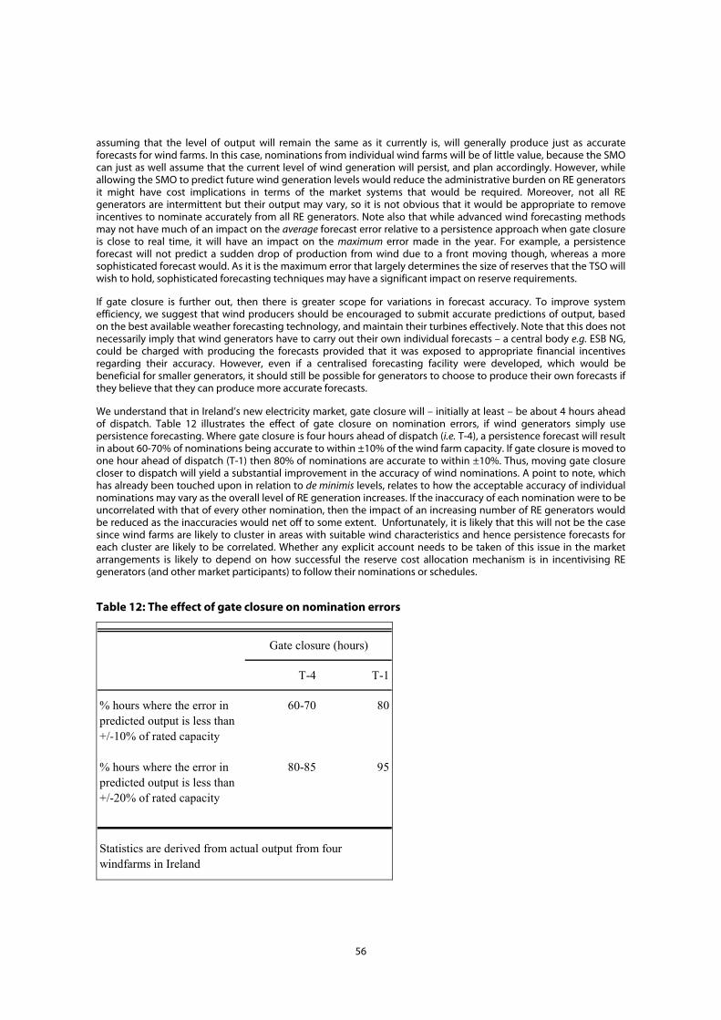
Table 12: The effect of gate closure on nomination errors 56

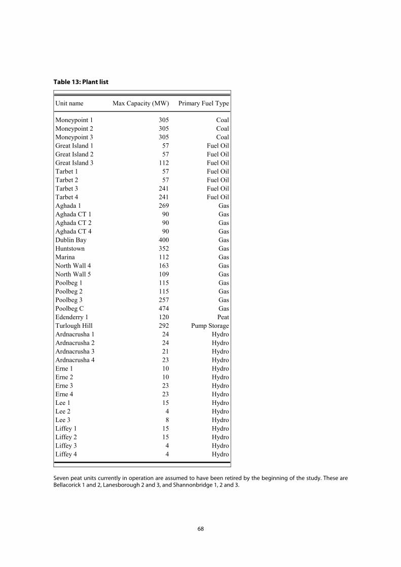
Table 13: Plant list 68

Table 14: New build plant (non-RE) 69

Table 15: Load Growth 70

Table 16: CO2 Unit emission rates 71

Table 17: Example heat rates 72

Table 18: Example Operating Costs 72

Table 19: Numerical example of RE FTR 80

Table 20: Effects of support mechanisms on desired offer floor price 82

Table 21: Cost Recovery Methodologies in US Electricity Markets 88

List of Figures

Figure 1: Min, Max and average monthly LMPs for wind nodes in 2006 10

Figure 2: Monthly price volatility at wind nodes for 2006 11

Figure 3: Monthly revenue and production for Donegal (normalised) 12

Figure 4: Min, Max and average monthly LMPs for wind nodes in 2009 15

Figure 5: Illustrative LMP price formation 15

Figure 6: Varying subsidies from PPA support as the LMP changes 23

Figure 7: The effect of different support mechanisms on prices at Mayo 24

Figure 8: Effect of a drop in LMP on revenues 27

Figure 9: Effect of a capacity-based FTR on revenues at Limerick 29

Figure 10: Effect of an RE FTR on revenues at Limerick 31

Figure 11: Example of cash flows for existing AER contracts under the new MEA 32

iii

Figure 12: Cash flows if another supplier ‘buys’ an AER contract from ESB CS 33

Figure 13: Revenue and production at Leitrim 34

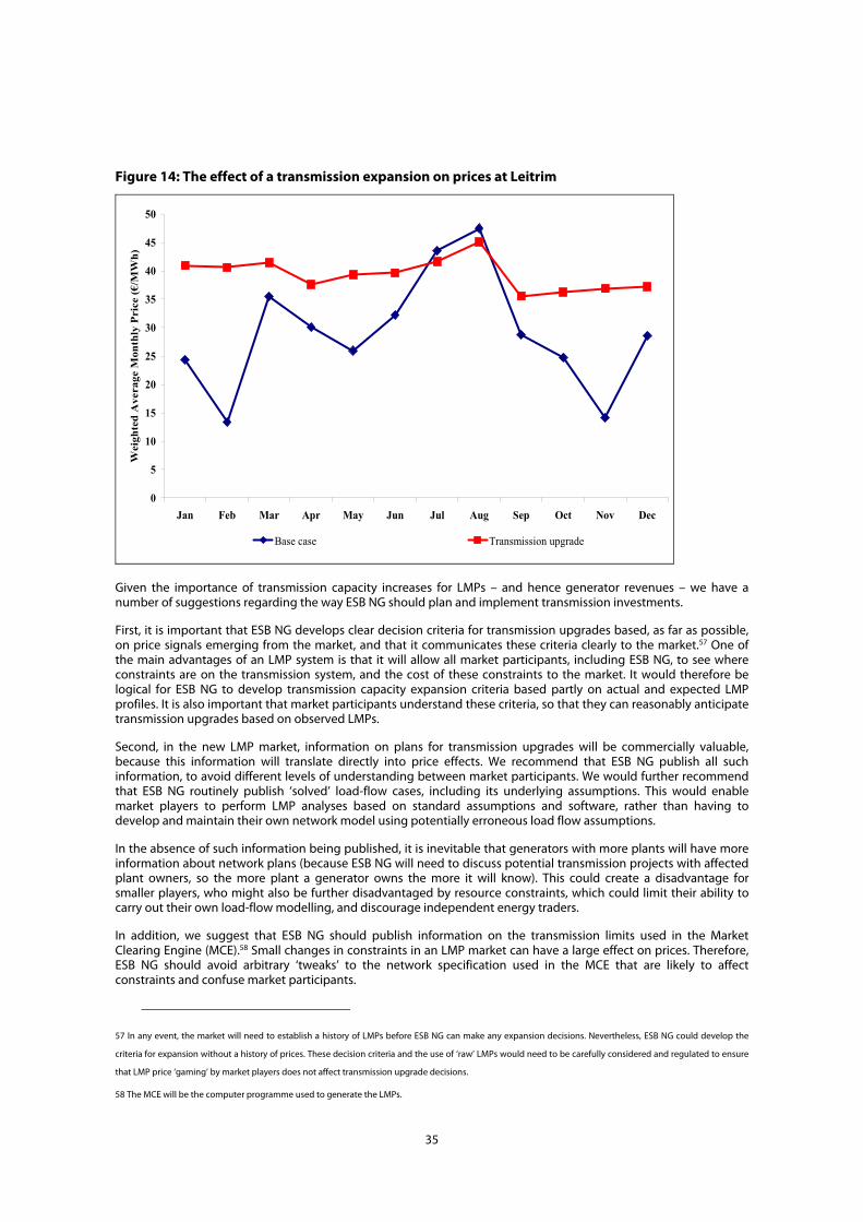
Figure 14: The effect of a transmission expansion on prices at Leitrim 35

Figure 15: Effect of greater dispersion on the prices received by RE generators 37

Figure 16: Price depression with a zero offers from RE generators 41

Figure 17: Price increases with must run RE generators offering at SRMC 42

Figure 18: Price distortions with PPA/FTR and regulated offers 42

Figure 19: Relationship between negative prices per month and revenue per month 46

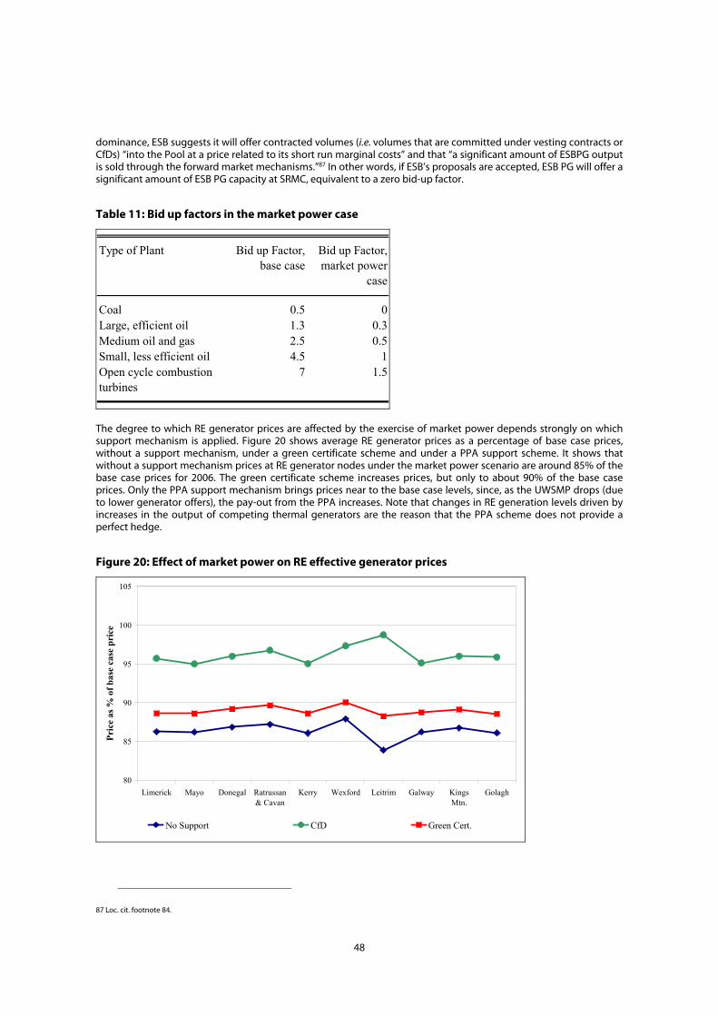
Figure 20: Effect of market power on RE effective generator prices 48

Figure 21: Allocating Contingency Reserve using the “Runway” model 54

Figure 22: Bids and costs at different load levels 65

Figure 23:Example of the summer hourly load shape – June 7, 2003 70

Figure 24: Forecast distribution of load at summer and winter peaks for 2007 73

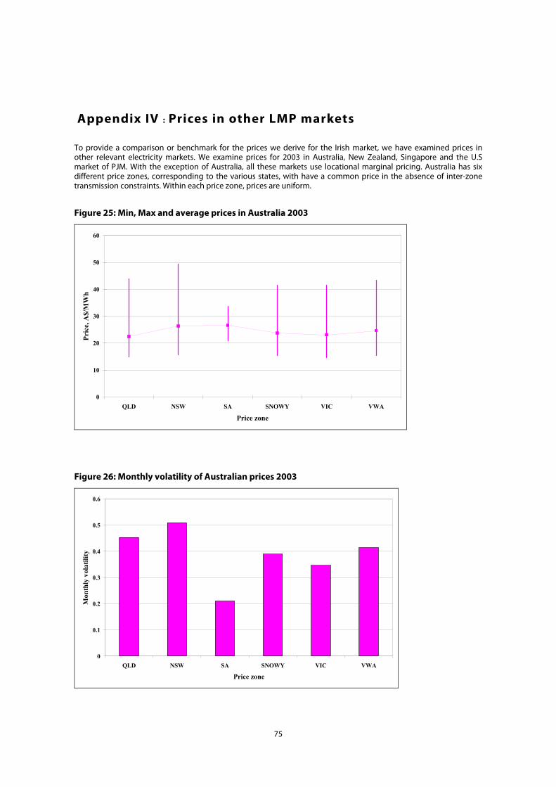
Figure 25: Min, Max and average prices in Australia 2003 75

Figure 26: Monthly volatility of Australian prices 2003 75

Figure 27: Min, Max and average prices in Singapore 2003 76

Figure 28: Monthly volatility in Singapore power prices for 2003 76

Figure 29: Min, Max and average prices in PJM 2003 77

Figure 30: Monthly volatility in PJM 2003 77

Figure 31: Incidents of negative prices per node in PJM 2003 78

Figure 32: Min, Max and average prices in New Zealand 2003 78

Figure 33: Monthly volatility in new Zealand for 2003 79

Figure 34: Income to an RE generator as a function of his LMP 81

Figure 35: Impact of wind on load factors 86

Figure 36: Impact of wind generation on number of starts 86

Figure 37: Impact of wind generation on ramping 87

1

1 Introduction and Summary

The Commission for Energy Regulation (CER) is working towards implementing new Market Arrangements for Electricity (MAE) for Ireland in 2006. Sustainable Energy Ireland (SEI) has commissioned The Brattle Group and Henwood Energy to study the impact that the MAE might have on Renewable Energy (RE) generators1 and combined heat and power (CHP) generators and to suggest features that might appropriately improve their position. In parallel, SEI has commissioned three other studies; one examines the effect of increased RE generation on the cost of reserves2, another discusses alternative financial support mechanisms for RE generators3 and the final one considers the position of distribution-connected RE generators.4

The purpose of this report is to inform the debate regarding RE generation under the new MAE. We identify key policy areas that are yet to be finalised, and consider the implications of different approaches to them for RE generators and CHP plants, supporting the discussion with quantitative modelling. Our aim is to develop options for various areas of market design, which market participants can then debate. It is important to note that the quantitative modelling we have carried out is only intended to illustrate the issues that we are discussing. The scope of the study did not include providing detailed wholesale price forecasts and we have not attempted to do so.

Whilst a detailed structure for the MAE has been developed, the CER has recently put the implementation of the MAE on hold for several months so that it can be reviewed in the light of comments received from market participants. At present, the intention is that the new MAE will be based around a compulsory market, with Locational Marginal Pricing (LMP), and references to the MAE in this report should be construed in this way. All generators above a minimum or de minimis level will receive the price at their relevant node, and customers will pay the calculated Uniform Wholesale Spot Market Price (UWSMP). The UWSMP will be the volume-weighted average of the prices at all the demand nodes. A list of the key documents that the CER has published on the market arrangements is included in Appendix I. As agreed with SEI, we have taken these decisions as “givens” in our study and have not sought to explore in detail what would happen if these aspects of the market rules were changed. However, most of our suggestions and ideas would be applicable in any form of gross pool market. Therefore, regardless of the final form of the market, the issues we address in this report will remain pertinent, and our conclusions and policy recommendations are largely independent of what type of compulsory market is eventually implemented. We highlight the relationship between our main findings and the form of new Irish market at the end of this summary.

Taking the proposed MAE rules as a given, several important policy areas relevant to RE generators remain open to question and debate. For example:

• How will different support mechanisms affect the position of RE and CHP generators under the MAE?

• Which RE generators will be exposed to LMPs?

• Will and, if so, how will, information requirement provisions vary with size?

• How will the cost of reserve be allocated? How can wind generators participate in the reserve market?

• Do wind generators need special protection against the possibility of negative prices, given their limited ability to control output?

• How should the concept of priority dispatch for RE generators be interpreted?

Our work addresses these and other issues. During the preparation of this study we have consulted with the CER, ESB National Grid (ESB NG) and various market participants. The interim version of this report was distributed to the CER’s expert group on RE generation, who gave valuable and constructive feedback. We would like to thank all parties consulted for their contributions to this report. In particular, we would like to thank ESB NG for the help it gave us in

1 In this report, we interpret RE as electricity generated from wind, waves, small-scale hydro, waste (including heat waste), biofuels, geothermal sources, fuel cells,

tides, solar cells and biomass.

2 “Study on operating reserve requirements as wind power penetration increases in the Irish electricity system”, ILEX Energy/UCD/QUB/UMIST, forthcoming from

SEI.

3 “Study on the Economic Analysis of RE Support Mechanisms” Energy Economics Group at Vienna University of Technology (EEG), forthcoming from SEI.

4 “Costs and Benefits of embedded generation in Ireland” PB Power, forthcoming from SEI.

2

assembling the data necessary for our modelling and the various Irish wind generators who allowed us to use helped in particular with obtaining data on their electricity production.

Various documents have already addressed the effect of the new market arrangements on RE generators. For example, in April 2003 the CER issued a document discussing the new trading arrangements and RE generators5, to which SEI responded in May 2003.6 More recently, CER issued a consultation document examining the implications of the detailed design of the new market arrangements on RE generators.7

We recognise that many readers will be interested in issues we do not address in this report, such as the absolute level of prices in the MAE; whether an LMP market is the ‘best’ market for the Republic of Ireland (RoI) and if market power will be exercised in the MAE. Whilst we accept that these are relevant and interesting questions for market participants, they lie outside the scope of the study. Instead, we use modelling to highlight the relative importance of policy choices and their robustness under different circumstances and scenarios and readers should bear this in mind when considering the analysis we have undertaken.

1.1 Structure of the report

To provide a context for the discussions that follow, we begin by describing the results from our LMP model runs (section 0). We explain the basic inputs of our model and how it works before examining the average level and volatility of prices at the nodes on the network where wind is likely to locate. We then discuss some alternative financial support mechanisms for RE generators (section 4), and the effect that these mechanisms would have on smoothing earnings for RE generators. Next, we discuss a group of issues that affect siting decisions and investment for RE generators (section 5), before going onto consider issues related to market operation, such as the dispatch of RE generators (section 6). Finally, we discuss how the cost of system reserve could be allocated in the market (section 7) and describe how wind generators could participate in the reserve market (section 8).

The report focuses primarily (but not exclusively) on wind generation, for two reasons. First, wind is expected to make up the majority of future RE generation build, at least in the medium term. Second, the operating characteristics of wind are markedly different to conventional thermal plant and some other RE plant types such as biomass – in that wind plants have very low marginal costs but are hard to schedule reliably far in advance (although they may well be controllable in the short-term). Consequently, some market rules may inadvertently discriminate against the different operating characteristics of wind plants, while other forms of RE generation that have characteristics similar to thermal plant (such as biomass) will be unaffected. Therefore, the special features of wind energy demand the most attention in this report.

As regards CHP generators, it is difficult to identify specific characteristics that apply to all such installations apart from their provision of steam for on-site processes. Some CHP plants will behave in a very similar manner to conventional thermal plant because their on-site steam (and electricity) demand is very stable whilst others, whose on-site requirements is unpredictable, may be more akin to wind generators. Consequently, we consider that most of the issues of relevance to CHP generators will be covered by considering the market from the perspective of both thermal generators and wind generators.8

1.2 Principal Findings

Prices in the MAE

We have estimated prices under a base case at all nodes in the MAE for 2006 and 2009. In 2006, the annual average price at likely wind nodes is 43.3€/MWh,9 essentially the same as the average price for generators. By 2009, the price received by wind generators under the base case rises by around 15% from 2006 levels, to an average of 49.6€/MWh (around half the price rise is due to inflation). This is below the average price received by all generators in 2009 of

5 CER/03/099, “Trading arrangements and renewables”, 30 April 2003.

6 Response to CER Document CER/03/099: Trading arrangements and renewables (30 April 2003).

7 CER/03/253, “Implementation of the market Arrangements for Electricity (MAE) in relation to Renewables, CHP and Distribution-connected Generation, An MAE

Consultation by the Commission for Energy Regulation Under S.I. 304 of 2003”, 10 October 2003.

8 We also note that DCMNR has set up a CHP strategy group, that is currently examining CHP-related issues in the MAE.

9 All prices in this report are presented in nominal terms.

3

50.9€/MWh. Of course, these prices are the result of a specific set of scenario assumptions and different scenario assumptions could lead to different outcomes. Nonetheless, we consider that our base case represents a credible outcome, given the structure of the electricity market in Ireland and current market views on the development of generation, demand and fuel prices, particularly as our modelling is only intended to identify those issues that are likely to be of most importance to RE generation. While we have calculated prices on the basis of an LMP market, the introduction of a gross pool10 would have relatively little effect on average prices. For example, we calculate that average gross pool prices in 2006 and 2009 would be 45.5€/MWh and 48.1 €/MWh respectively. The similarity in prices is largely due to the absence of significant transmission constraints in the Irish market.

Overall, our analysis suggests that the monthly price volatility under the MAE may be low relative to volatility levels seen in other LMP markets such as New Zealand, PJM in the U.S. and Singapore. (However, this result should be treated with some caution as it may be, in part, a modelling artefact.) The monthly revenue volatility for wind generators is higher – revenues vary from around double the average monthly revenue to half – due to changes in production levels.

The transmission system operator currently uses Transmission Loss Adjustment Factors (TLAFs) to account for system losses by adjusting the production credited to a generator. The effect of the TLAFs can equally be thought of as imposing discounts or premia on the prices/revenues that a generator earns relative to the price paid by consumers.11 We calculate the equivalent discounts and premia that would apply under the MAE (in this case, specified as the ratio between a generator’s LMP and the UWSMP). Whilst the methodologies used to derive the two sets of adjustments are inevitably different12 (and hence it is not surprising that the outcomes are different), the comparison is relevant because in each case the adjustment factor measures an individual generator’s position compared with that of a generic consumer. Our analysis suggests that many of the wind nodes that currently attract a premium will, under the MAE, face a discount. This implies that the locational signal at these nodes have changed direction or ‘flipped.’ This does not imply that the current methodology for calculating TLAFs is ‘wrong’, simply that a different market mechanism could well result in different locational signals from those seen at present. Note that if a gross pool were to be introduced, as opposed to an LMP market, ESB NG may continue to apply TLAFs to provide locational signals.

Support mechanisms

While it is not the aim of this study to discuss the pros and cons of alternative support mechanisms, the choice of support mechanism affects many of the key policy issues. Consequently, a discussion of whether any explicit market design features are required to facilitate RE generation must take account of potential support mechanisms. The support mechanisms discussed in this report are only developed in outline, and the detailed rules, which would be required in practice, could effect RE generator behaviour.

We understand that a typical wind generator requires around 55€/MWh to recover its full costs, including a return on capital employed.13 Therefore, the prices we estimate for 2006 imply a revenue shortfall of around 5-10€/MWh for wind generators. Consequently, some form of financial support mechanisms for RE generators may be required in the MAE, at least in the short term.

We describe several forms of support mechanism, and examine two – a Power Purchase Agreement (PPA) scheme (in which RE generators hold contracts for differences – CfDs – whose volumes always exactly match their output and whose contract price enables them to cover their costs), and an green certificate scheme with supplier obligations on green power purchases – in detail. As noted above, we estimate that subsidies required by wind producers would be about 10€/MWh in 2006, but this would fall to less than 0.5€/MWh by 2009 as market prices rise.14 This implies that there is a strong need for support in the early years of the new market, but that any support mechanism should be responsive to rising market prices to avoid excessive subsidies to RE generators, especially if the cost of RE technology falls.

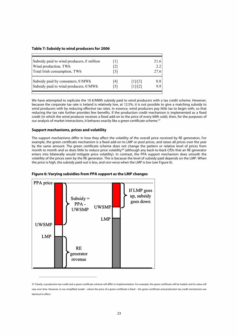
The two support mechanisms considered differ in two important respects. First, PPA based schemes are able to smooth prices and revenues. In contrast, a green certificate scheme is simply an add-on to market prices, and does

10 By gross pool, we mean a market where the same price is paid to all generators.

11 In other words, the price paid at a lossless node.

12 The principles underlying the two methodologies are described in section 2.1.

13 This value is consistent both with the prices achieved in the most recent AER round and with values quoted to us by wind developers.

14 Assuming the revenue required by generators does not change in nominal terms.

4

nothing to dampen any volatility that may exist. (Of course, there is nothing to stop RE generators signing CfDs with the same suppliers to whom their green certificates are sold. However, the characteristics of such a CfD are likely to be very different to a price support PPA). Reduced revenue volatility could help finance new RE projects. Second, the level of subsidy (i.e. the amount that RE generators receive for their electricity, over and above the market price) under a PPA scheme will automatically reduce as market prices increase, while, in its simplest form, a green certificate subsidy is independent of market prices. Consequently, subsidies under a PPA based scheme could be easier to manage, especially if prices rise over time, as our modelling predicts.

Siting decisions and investment

We argue that, in general, exposing RE generators to LMPs should help to facilitate efficient siting decisions and minimise the costs of congestion and network expansion. We note that, as the UWSMP is around 5% higher than the average generator LMP, paying RE generators connected to the distribution grid the UWSMP would distort connection incentives. However, exposing RE generators to nodal prices introduces financial risks to RE projects. For example, the LMP at a particular node could fall sharply due to congestion.

RE generators can protect themselves against the risk of low LMPs at their nodes by buying Financial Transmission Rights (FTRs). Some market participants submit that a capacity-based FTR is worth less to wind generators because their load factor is typically lower than that of a thermal generator. We note, however, that the intrinsic value of an FTR is the same for both types of generator and this suggests that RE generators should not pay less for capacity-based FTRs except as part of a support mechanism. However, by acquiring capacity-based FTRs, RE generators enter into an obligation to pay out on the FTR, while they have no certainty of a contemporaneous income stream from electricity generation that will offset the obligation. This could result in negative revenues for wind generators in some periods. Our analysis suggests that, in practice, this is unlikely to occur. Nevertheless, the issue could present a problem when financing new wind projects, especially in the early years of the MAE where there is little history of LMPs. Lenders may require an RE generator to hold an FTR to protect against the risk of low LMPs, but also worry that this could result in negative revenues if the relevant LMP is high at times when the wind farm is not producing.

If this possibility is considered to be too great a risk, we have developed an alternative to capacity-based FTRs for RE generators (which we call RE FTRs) that overcomes this problem as part of a support mechanism. Pay-outs under the RE FTR are based on produced energy – rather than capacity – but, in return, the RE generator is not fully hedged against nodal prices, so that some locational signal remains.

We describe ways in which the existing AER contracts could be dealt with under the MAE, and note that it is important to respect the principles underlying these agreements to foster investor confidence in the new MAE. We also describe how the existing AER contracts could be made available as financial hedging tools to market participants other than ESB Customer Supply.

Under the MAE, transmission upgrades will have significant effects on prices at individual nodes. We conduct a case study on one of the wind nodes that our analysis suggests is likely to be congested (Leitrim), and demonstrate that a transmission expansion at this node increases LMPs by nearly 50%, assuming there is no locational market power. If investors are to have confidence in the MAE, it is important that transmission expansion decisions are made in a transparent manner. This will avoid seemingly ‘random’ changes in prices, due to unexpected changes in transmission constraints, which would undermine investor confidence. Ideally, the criteria for transmission expansions should be published. This will help market participants understand how prices will evolve as the grid expands. We describe the transmission expansion procedure in PJM as an example of transparent planning in an LMP market, although we recognise that there are differences in scale between the two markets that may make some of the PJM procedures inappropriate for the Irish market.

Market Operation

The concept of priority dispatch for RE generators can be interpreted in a number of ways and is a topic that has attracted much debate in the Irish market. We consider three interpretations: (1) ‘no impediment’, where the SMO dispatches RE generators on the basis of offers, but ensures no discrimination against RE generators; (2) a ‘must run’ requirement with market offers, where the offers of RE generators are set at a level that ensures dispatch, or the SMO dispatches them regardless of their offer; and (3) subtracting RE generation from load.

We conclude that with a must-run interpretation, the CER should regulate the offers of RE generators. However, regulated prices combined with a must-run requirement will distort market prices, and the resulting prices could be above or below their free market level, depending on the way the CER sets RE generator prices. Similarly, subtracting RE generation from demand before other generators are scheduled will depress market prices. Only the no-impediment interpretation, as applied by the GB energy regulator (Ofgem), will not distort market prices. However, this interpretation could mean that cheaper non-RE plant would sometimes be dispatched in preference to higher marginal cost RE generators.

5

The CER has proposed that whether RE generators have to participate in the market i.e. be paid the relevant LMP, have to provide output forecasts and be directly exposed to reserve costs, or self-dispatch (and be paid the UWSMP) should depend solely on their size. We separate out consideration of the pricing rules from those governing information provision and propose a number of alternative criteria for these decisions. We suggest that an expansion of the concept of a trading site, where generation and demand are netted off from one another for settlement purposes, might be helpful. We also consider dynamic de minimis levels for providing information to the TSO, so that as developers install more wind generation in a zone, they must provide more information to the SMO. A Public Service Obligation charge could recover the costs of any additional information provision requirements imposed on plant developers after they made their investment decision.

Many wind generators are concerned at the prospect of negative prices, which can occur in LMP markets and some gross pool markets. Some wind generators may be unable to turn-off during periods of negative prices, and consequently may have to pay to produce. However, our modelling produced no negative prices at likely wind nodes. Moreover, for the system in general, we find no correlation between negative prices and low monthly generator incomes, implying that negative prices are random events. While negative prices do not appear to be a problem in practice, we describe several methods of providing assurance to RE generators on this issue, if this is required. We note that generators are less likely to experience negative prices in a gross pool than in an LMP market.

Market power is an important issue in the Irish market. While it is beyond the scope of this report to investigate market power issues in detail, we do simulate a scenario where the vertically integrated incumbent, ESB, reduces wholesale prices to around 85% of our base case 2006 prices. Such an exercise of market power would be more harmful to RE generators than an increase in wholesale prices and may, in any case, be more likely, given the current proposals for vesting contracts. The degree to which low prices affect RE generator prices depends on the choice of support mechanism. With a green certificate scheme, prices in this scenario are reduced to around 90% of what they would have been without market power. In contrast, the PPA support mechanism compensates almost completely for the low prices, insulating RE generators against market power.

Reserves

Intermittent RE generators, such as wind, may increase the amount of reserve required.15 As the CER’s intention is that the cost of reserve should be allocated on a ‘causer-pays’ principle, this could result in increased costs for wind generators. Moving gate closure nearer to dispatch as soon as possible should reduce forecasting errors associated with wind production, and reduce reserve costs.

We develop a methodology for allocating the cost of frequency reserve (required to compensate for small continuous deviations in off-take and generation). In any settlement period, the cost of frequency reserve incurred for that period should be divided among the market participants (i.e., loads and generators) in direct proportion to the degree to which their deviations from schedule are correlated with the total system deviation from schedule. If a generator’s deviation is in the opposite direction to the rest of the market, then we suggest that they should not pay for frequency reserve in that period.

The cost of contingency reserve – required when a major source of generation in the system is lost – could be allocated based on the contribution each generator makes to the need to hold contingency reserve. This depends on a generator’s size relative to other units in the market and its short-term forced outage rate. Such a methodology for sharing the cost of contingency reserve, would be likely to result in RE generators paying less than has been suggested in the past.

We see no reason why intermittent RE generators such as wind should not be able to offer reserve to the SMO. To a degree, the PJM market has already set a precedent for this by giving installed capacity credits to wind generators. The SMO could ‘discount’ reserve offers from wind generators, to make them as reliable as reserve offers from thermal plant. For example, we calculate that a wind farm operating at 50MW in hour t could offer 35MW of reserve in hour t+1 (by turning current production down to zero), and be at least as reliable a source of reserve as a thermal plant. We recommend establishing discounting rules to allow RE generator participation in the reserve market, and moving gate closure as close as possible to dispatch to avoid excessive discounting of reserve offers from wind.

Alternative market forms

As already noted, the CER has recently suspended implementation of the MAE, and issued a questionnaire to market participants that invites them to challenge some of the fundamental assumptions of the proposed MAE. The implication is that the final form of the new Irish market may not be an LMP market, but rather some form of pool

15 This issue is being investigated in detail in a separate study, see footnote 2.

6

market with a single price, as opposed to many nodal prices. Given that we have carried out our study assuming an LMP market, this naturally raises the question as to which of our policy recommendations remain valid in the absence of an LMP market.

Table 1 summarises the subject areas of our main findings and recommendations, and outlines the effect of an alternative market arrangement. The alternative market we consider is a gross pool i.e. a compulsory pool, similar to the England and Wales market before the introduction of the New Electricity Trading Arrangements (NETA). Generators must offer into the pool, and consumers or their suppliers must buy from the pool. The pool generates a single price, being the highest accepted generator offer price. All generators receive this price, although the output for which they are paid may be adjusted by location-specific loss factors. Buyers pay the price that generators receive. The Transmission System Operator (TSO) manages constraints and losses outside the pool. The TSO can schedule spinning reserve within a gross pool or contract it separately.

Table 1 illustrates that, with the exception of some LMP-specific issues such as FTRs, an alternative form of market would have little effect on our main findings and recommendations.

Table 1: The effect of an alternative market form on our main recommendations

Subject of recommendation/finding Effect of a gross pool on recommendations/findings

Level of prices in the LMP market Our calculations indicate that the average LMP price is almost identical to the price which would result from a gross pool. This is because there are relatively few transmission constraints in the Republic. Therefore, average LMP prices can be read as a pool price. Because the finding that some types of RE generators may require a support mechanism is based on average LMP prices, this finding would be unchanged if a gross pool market was implemented. However, a pool will solve the issue of some constrained nodes experiencing low prices.

Support mechanisms Our findings are unaffected: subsidies under a PPA based scheme would still be easier to manage in a gross pool.

Siting decisions A gross pool would eliminate the problems with FTRs that we highlight, and negate the need for an alternative FTR. Transmission upgrades would be less important, though could still affect generator revenues via TLAFs.

Priority despatch and de minimis levels No effect

Negative prices Assuming negative prices were allowed, they would be very unlikely to occur in a gross pool. However, our conclusion is that negative prices are also unlikely to materially affect RE generators in the LMP market, so our conclusions remain unchanged.

Market power Our conclusions are unaffected: market power will remain an important issue in any market design.

Reserves No effect

Conclusions

Our analysis suggests that the priority that has, until now, been attached to some issues (intermittency, FTRs, negative prices etc.) by RE generators may be undue since there are others (support mechanisms, transmission planning) that are likely to be more important for them. However, our study has not indicated any problems that would jeopardise the future of RE generators under the MAE, particularly given the likely support mechanisms. Nonetheless, there is room for improvement in some areas of market design.

7

Further work

There are a range of further policy issues relating to the MAE that would benefit from a mix of policy analysis and quantitative modelling similar to that applied in this study. For example, the planned Ireland-Wales interconnector may have important implications for RE generators. In addition, further regional integration of electricity markets, exemplified by the moves towards an all-island market, will present new challenges and areas for discussion. For example, the potential for an integrated market for ROCs across GB, Northern Ireland and the RoI is a development that would be worth further investigation in future. Further quantification of the impact of different reserve allocation mechanisms would also be useful.

The CER and ESB NG have set up a Market Modelling Project, which is designed to explore the impact of various possible market designs. Areas that it would be useful for this project to consider include:

• The impact of different strategies regarding generator offers, including an analysis of the effect of the regulation of ESB’s behaviour on market prices.

• Additional load flow analyses, for different times of the year (to capture different line loadings and demand distribution), and for different years.

• More detailed analysis of the impact of different market designs.

8

2 Prices in the MAE in 2006 and 2009

We have used the sophisticated quantitative market model suite developed by Henwood Energy Services to help inform the discussion surrounding some of the outstanding policy issues in the market. Henwood’s software is used by over 150 power industry participants worldwide. Moreover, the optimisation algorithm used (MARKETSYM LMPTM) is used on a daily basis to calculate top-up and spill prices for the current Irish market.

The objective of the modelling was to identify those issues that are likely to have a substantial effect on LMPs and generators’ incomes, so that more effort can be devoted to examining these issues. Therefore, we are more interested in the differences between prices under various scenarios than the absolute level of prices. Nonetheless, we have sought to produce a credible base case scenario for 2006 and 2009. However, the modelling we undertook utilised Henwood’s standard modelling approach, developed through extensive modelling assignments in liberalising power markets worldwide, including both LMP and gross pools. (Appendix II explains Henwood’s approach to modelling in detail.)

It is worth noting that our modelling approach automatically generates both gross pool and LMP prices. The initial step is to model a gross pool market and the outputs from this are then fed into our load flow model to produce LMPs. In other words, our assumptions, inputs and outputs are valid for both gross pool and LMP market structures. To illustrate this point, gross pool market prices have been provided in this report alongside the equivalent LMP prices where relevant.

Our modelling has naturally focused on the RoI. However, the RoI is interconnected with Northern Ireland and by 2009 (it is assumed) with Wales. To inform our RoI analysis, Henwood performed full gross pool runs of an all-island market, and of the GB market, the key results of which are outlined in Appendix III.2.

Readers should note that all price forecasts are subject to significant and unquantifiable uncertainty. For example:

• The exercise of market power could move wholesale prices substantially up or down from competitive levels, but whether market power can be exercised will depend on the regulatory policies of the CER;

• We have assumed that the distribution of loads across the network (but not their absolute levels) remains the same as the distribution at the summer-peak throughout the year and over time.16 We made this assumption only because no other data were available to us at the time the modelling was carried out ();

• Fuel prices could change significantly, either up or down;

• Demand could be higher or lower than expected;

• Grid upgrades and/or extensions will, over time, be brought on-line which we have been unable to model.

All the factors listed above, and others, could significantly affect prices. We have attempted to capture some of the uncertainty in prices by modelling several alternative scenarios – varying parameters such as market power and transmission constraints. The use of scenarios is a well-established method of exploring uncertainty.17 However, we have not attempted to explore the plausible range of outcomes but instead have concentrated on outcomes that would be detrimental to renewable generation since these are most relevant to policy considerations. We accept that it is unlikely that any two parties will agree on any set of modelling assumptions, which are by definition subjective, but we do not consider that adopting different modelling assumptions would be sufficient to undermine our policy conclusions.

We report prices for each of the years in the following sections, before giving more detail on the modelling approach and assumptions. Note that the LMP model generates a price at each node for every hour in the year and consequently we often need to aggregate prices to provide a clear picture. When the nodal prices are aggregated to a market level, they approximate the prices that a gross pool would generate. Except where stated otherwise, we report production-weighted averages as opposed to straight time-weighted average. Production-weighted prices are

16 Figure 24 in Appendix III illustrates that the simplicity of this assumption is unlikely to have materially affected our results in 2006.

17 There are, of course, other methods of measuring uncertainty, such as error bands and confidence intervals. However, “error bands” derive from scientific

experiments, typically where measuring equipment has a known margin of error. Random processes generate confidence intervals. Consequently, it is extremely

unusual for electricity price projections to incorporate error bands or confidence intervals.

9

useful, because multiplying them by production gives a generator’s revenue i.e. they can be thought of as generator revenue normalised for production.18 We concentrate on average monthly prices because most generators pay expenses such as interest repayments on a monthly basis. All prices quoted are in money-of-the-day.

It should be noted that, in the 2006 and 2009 cases, all units are dispatched purely based on their offers – no dispatch priority has been assumed for any generator. However, low marginal costs have been assumed for peat plant to mimic must-run operation and wind generators naturally have low marginal costs so that, in most instances, these plant run whenever they are available.

2.1 2006 Prices

Key assumptions for 2006

• A total of 650 MW of wind capacity is installed at 11 different nodes around Ireland.19

• Both Tynagh Energy CCGT and Aughinish CHP are commissioned by the start of the year;

• A baseload interconnector flow from Northern Ireland of 167MW20 continues until August 2006, under the

existing contract between ESB and Ballylumford;

• An additional peak flow from Northern Ireland of 50MW is assumed until the end of August, with flow for

the final four months of 2006 at 200MW peak and 70MW off-peak; and

• The peak load is 4824MW for the RoI and total annual demand is 27.6TWh.

More details of the assumptions used are provided in sections 3.2 and 3.3, and in Appendix III. In general, we have sought to utilise information provided by the transmission system operator21 wherever possible and appropriate.

18 In contrast, a time weighted average price can be misleading, especially for intermittent generation. For example, the electricity price could be high in the

afternoons, but if a generator rarely produced in the afternoons, the high price would be of little benefit to the generator. The time-weighted price would appear

high, but this would give a misleading impression regarding the generator’s revenues. In contrast, the production-weighted price accounts for when the

generator produces electricity, and only gives weight to prices when the generator is producing.

19 To provide a context for the results presented in this report, Appendix VIII explores the impact on thermal generators of including wind farms in the Irish

capacity mix.

20 Current contracted volume, source: ESB

21 For example, the ‘Generation Adequacy Statement 2004-2010’ and the ‘Forecast Statement 2003-2009’.

10

3 Prices in 2006

Figure 1 illustrates the average, maximum and minimum prices at the main RE generation nodes, for each month of 2006. The average price received by RE generators at these nodes is 43.3€/MWh, essentially the same as the average price received by all generators (43.2 €/MWh). Using the same assumptions, a gross pool, similar to the one that used to exist in England and Wales, would produce an electricity price of 45.5 €/MWh. Low prices at Leitrim strongly influence the average price for RE generators. Excluding the Leitrim node, wind nodes receive an average price of 45.2 €/MWh. Prices at the Leitrim node were nearly 40% lower than the average RE generator price, and were only 1 €/MWh for 15% of the time.22 The reason is that this node is upstream of a frequent export transmission constraint, which causes the price to drop when it is active. Note that our analysis assumes that there is a competitive position behind the node. If this were not the case, then it would be possible to bid-up behind the constraint until the point at which imports became attractive and the constraint was relieved. However, throughout this study we assume that RE generators offer electricity at marginal prices and do not exercise market power.

It is interesting to note that prices in Donegal are comparable to those at other wind nodes, despite its relatively isolated position. However, this result confirms the LMP analysis that Ilex carried out for the CER.23

Figure 1: Min, Max and average monthly LMPs for wind nodes in 2006

0

10

20

30

40

50

60

Lim

eric

k

May

o

Don

egal

Rat

russ

an &

Cav

an Ker

ry

Wex

ford

Lei

trim

Gal

way

Kin

gs M

tn.

Gol

agh

Wei

ghte

d A

vera

ge M

onth

ly P

rice

(€/M

Wh)

Our modelling does not generate any negative prices at wind nodes. Indeed, it only produces 140 negative prices in total out of some 3 million prices,24 with the lowest price being -46 €/MWh.

Our analysis suggests that prices under the MAE may be less volatile than those in other LMP markets in the world (Figure 2 shows monthly price volatility at wind nodes).25 In part, the lower volatility values we have found may be a result of our modelling only a limited number of days and having to base all our runs for 2006 on a single load-flow case (discussed in more detail in section 3.2 and Appendix III), but it also reflects the fact that the Irish grid is

22 €1/MWh is the “nominal” bid price for all wind generators. No gaming at nodes is assumed; for more details on the bidding assumptions used for the study see

Section 2.3

23 ‘The price and dispatch impact of a centralised wholesale market in Ireland’, Ilex/UMIST/UCD, April 2003.

24 The model actually predicts 35 incidents of negative prices, but as we only calculate prices for one week per month, we scale up the calculated incidents of

negative prices by a factor of four.

25 We calculate volatility as the standard deviation of the series (natural log of {average price in month M/log of the average price in month M-1}

11

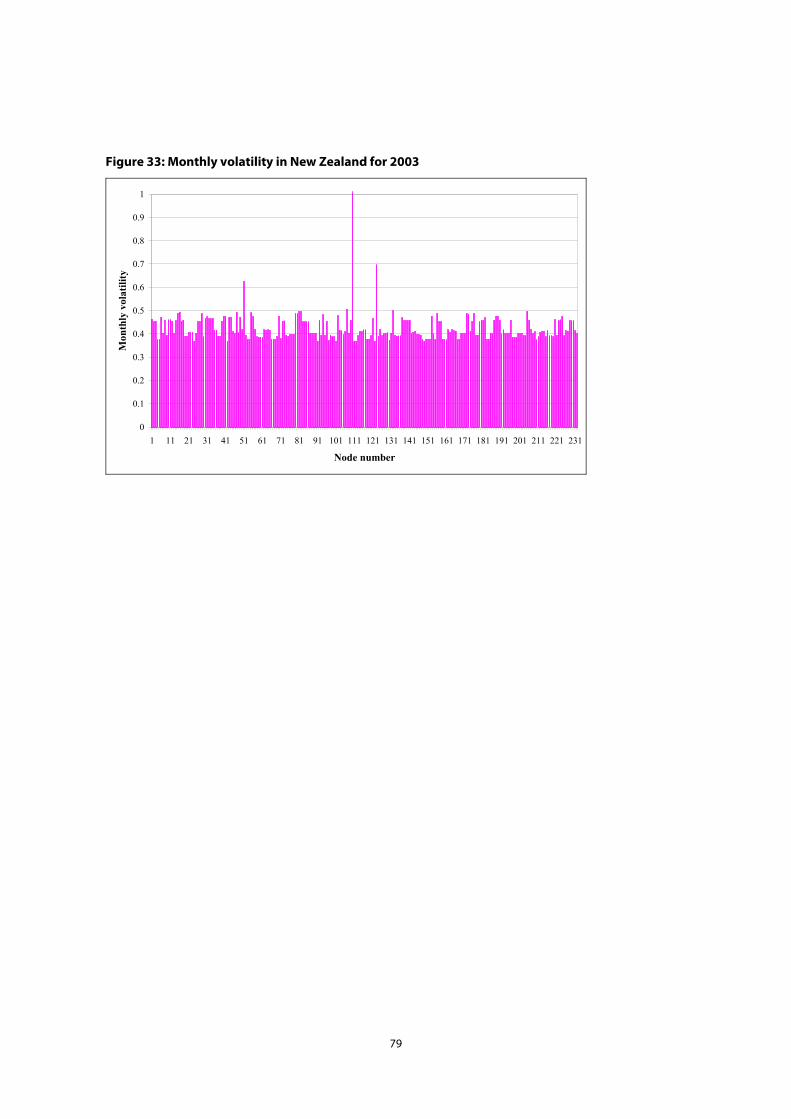
relatively unconstrained. Average price volatility in the MAE is around 0.13, although volatility at the Leitrim node is much higher at 0.51, again because of the constraints at this node. This level of volatility is somewhat lower than the monthly price volatility seen in Singapore’s LMP market in 2003, and about half the level of monthly price volatility in PJM (the largest LMP market in the world) for the same period. New Zealand’s LMP market in 2003 had an even higher level of monthly volatility, with most nodes experiencing a monthly volatility of around 0.4. (For more detail on prices in other LMP markets, see Appendix III).

The volatility of prices we have calculated assumes that the market will have settled down after the introduction of the MAE. Based on experience of other markets that have moved from one design to another, Ireland is likely to witness a relatively short, transitory period of high price volatility following the implementation of any new trading arrangements, be they a gross pool or an LMP market.

Figure 2: Monthly price volatility at wind nodes for 2006

0.00

0.10

0.20

0.30

0.40

0.50

0.60

Limeri

ckM

ayo

Doneg

al

Ratrussa

n & C

avan

Kerry

Wex

ford

Leitrim

Galway

Kings M

tn.

Golagh

Vol

atili

ty

Monthly Revenue for wind generators

The revenue for wind generators varies considerably from month-to-month. However, changing production – rather than large monthly swings in LMP – is the main cause of these variations. Figure 3 illustrates the (normalised) revenue and production for Donegal, which is typical of most of the wind nodes studied, and shows that the profile of revenues tracks that of production closely. The exception to this is Leitrim, which, due to transmission constraints, experiences periods of high production but low revenue, as a result of low prices (we examine the Leitrim case in more detail in section 5.3).

12

Figure 3: Monthly revenue and production for Donegal (normalised)

0

20

40

60

80

100

120

140

160

180

200

Jan Feb Mar Apr May Jun Jul Aug Sep Oct Nov Dec

% o

f Ave

rage

Revenues Production

Changes in locational signals in the MAE

At present, ESB NG adjusts generator production for transmission losses by applying Transmission Loss Adjustment Factors (TLAFs) which vary by season (winter/summer) and time (day/night). The TLAF gives a locational signal to generators, because generators will prefer to site plant at a location with a high TLAF since they will be credited with more production than they actually produce. Although TLAFs adjust a generator’s production, their financial effect is equivalent to paying generators different prices at different locations. In an LMP market, the price at each node for each period automatically accounts for losses and constraints, and this generates a locational signal i.e. a node where generation gives rise to large losses or constraints is more likely to have a low price, and generators may prefer to site their plants elsewhere. We note that, regardless of the form of market design, losses and constraints must be dealt with. In the event that the new arrangements take the form of a gross pool, ESB NG may well continue to apply TLAFs calculated using the current methodology.

An interesting exercise is to compare the locational signals given to RE generators under the present market arrangements with the locational signals implied by the LMPs calculated in our modelling. Our model does not directly generate TLAFs26, but we can calculate whether a generator earns a premium or a discount on its electricity sales, relative to the market as a whole (UWSMP) so as to create a valid comparison with the impact of the current TLAFs. The premia and discounts factors are calculated as the ratio between the revenue that a generator would earn if it was paid UWSMP and the revenue that it earns when paid the LMP at its node. In other words, the factor is the number that when used to multiply revenues calculated using the UWSMP gives the correct generator revenue. Similarly, under the current system the TLAFs represent the factors that when used to multiply revenues calculated using a uniform (lossless) price give the correct generator revenue.

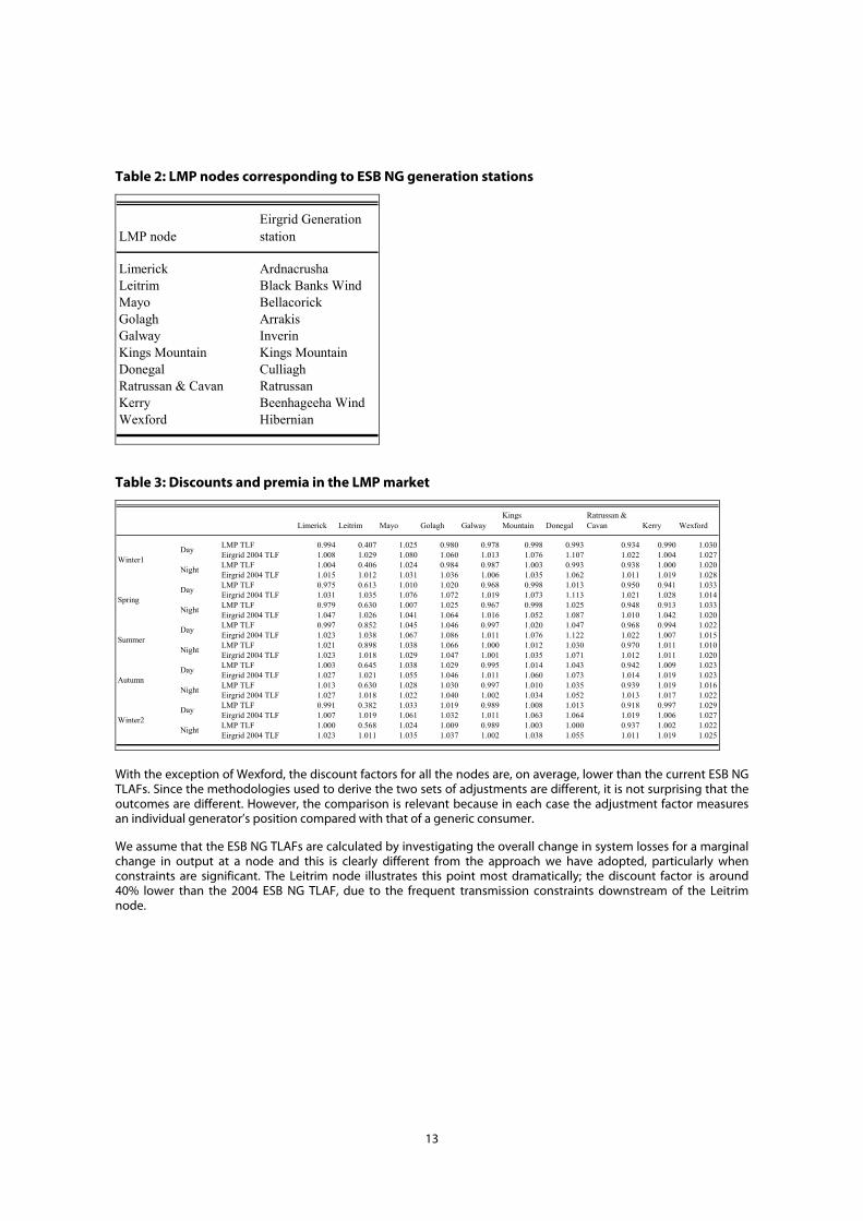
Table 2 shows which ESB NG TLAFs we used for comparison against our discount and premia factors. For example, we compare the premia/discount factor calculated for the Limerick node with ESB NG’s TLAF for Ardnacrusha. Table 3 compares the premia/discount factors with ESB NG’s 2004 TLAFs, for different periods of time and for all wind nodes.

26 Instead, they are implicitly included in the LMPs that it produces.

13

Table 2: LMP nodes corresponding to ESB NG generation stations

LMP nodeEirgrid Generation station

Limerick ArdnacrushaLeitrim Black Banks WindMayo BellacorickGolagh ArrakisGalway InverinKings Mountain Kings MountainDonegal CulliaghRatrussan & Cavan RatrussanKerry Beenhageeha WindWexford Hibernian

Table 3: Discounts and premia in the LMP market

Limerick Leitrim Mayo Golagh Galway Kings Mountain Donegal

Ratrussan & Cavan Kerry Wexford

LMP TLF 0.994 0.407 1.025 0.980 0.978 0.998 0.993 0.934 0.990 1.030Eirgrid 2004 TLF 1.008 1.029 1.080 1.060 1.013 1.076 1.107 1.022 1.004 1.027LMP TLF 1.004 0.406 1.024 0.984 0.987 1.003 0.993 0.938 1.000 1.020Eirgrid 2004 TLF 1.015 1.012 1.031 1.036 1.006 1.035 1.062 1.011 1.019 1.028LMP TLF 0.975 0.613 1.010 1.020 0.968 0.998 1.013 0.950 0.941 1.033Eirgrid 2004 TLF 1.031 1.035 1.076 1.072 1.019 1.073 1.113 1.021 1.028 1.014LMP TLF 0.979 0.630 1.007 1.025 0.967 0.998 1.025 0.948 0.913 1.033Eirgrid 2004 TLF 1.047 1.026 1.041 1.064 1.016 1.052 1.087 1.010 1.042 1.020LMP TLF 0.997 0.852 1.045 1.046 0.997 1.020 1.047 0.968 0.994 1.022Eirgrid 2004 TLF 1.023 1.038 1.067 1.086 1.011 1.076 1.122 1.022 1.007 1.015LMP TLF 1.021 0.898 1.038 1.066 1.000 1.012 1.030 0.970 1.011 1.010Eirgrid 2004 TLF 1.023 1.018 1.029 1.047 1.001 1.035 1.071 1.012 1.011 1.020LMP TLF 1.003 0.645 1.038 1.029 0.995 1.014 1.043 0.942 1.009 1.023Eirgrid 2004 TLF 1.027 1.021 1.055 1.046 1.011 1.060 1.073 1.014 1.019 1.023LMP TLF 1.013 0.630 1.028 1.030 0.997 1.010 1.035 0.939 1.019 1.016Eirgrid 2004 TLF 1.027 1.018 1.022 1.040 1.002 1.034 1.052 1.013 1.017 1.022LMP TLF 0.991 0.382 1.033 1.019 0.989 1.008 1.013 0.918 0.997 1.029Eirgrid 2004 TLF 1.007 1.019 1.061 1.032 1.011 1.063 1.064 1.019 1.006 1.027LMP TLF 1.000 0.568 1.024 1.009 0.989 1.003 1.000 0.937 1.002 1.022Eirgrid 2004 TLF 1.023 1.011 1.035 1.037 1.002 1.038 1.055 1.011 1.019 1.025

Day

Night

Day

Night

Day

Night

Day

Night

Winter1

Spring

Summer

Autumn

NightWinter2

Day

With the exception of Wexford, the discount factors for all the nodes are, on average, lower than the current ESB NG TLAFs. Since the methodologies used to derive the two sets of adjustments are different, it is not surprising that the outcomes are different. However, the comparison is relevant because in each case the adjustment factor measures an individual generator’s position compared with that of a generic consumer.

We assume that the ESB NG TLAFs are calculated by investigating the overall change in system losses for a marginal change in output at a node and this is clearly different from the approach we have adopted, particularly when constraints are significant. The Leitrim node illustrates this point most dramatically; the discount factor is around 40% lower than the 2004 ESB NG TLAF, due to the frequent transmission constraints downstream of the Leitrim node.

14

Table 4: Changes in the locational signal from the TLAFs in the MAE

Limerick Leitrim Mayo Golagh Galway Kings

Mountain Donegal Ratrussan &

Cavan Kerry Wexford

Day Flipped Flipped No flip Flipped Flipped Flipped Flipped Flipped Flipped No flipNight No flip Flipped No flip Flipped Flipped No flip Flipped Flipped Flipped No flipDay Flipped Flipped No flip No flip Flipped Flipped No flip Flipped Flipped No flipNight Flipped Flipped No flip No flip Flipped Flipped No flip Flipped Flipped No flipDay Flipped Flipped No flip No flip Flipped No flip No flip Flipped Flipped No flipNight No flip Flipped No flip No flip No flip No flip No flip Flipped No flip No flipDay No flip Flipped No flip No flip Flipped No flip No flip Flipped No flip No flipNight No flip Flipped No flip No flip Flipped No flip No flip Flipped No flip No flipDay Flipped Flipped No flip No flip Flipped No flip No flip Flipped Flipped No flipNight No flip Flipped No flip No flip Flipped No flip No flip Flipped No flip No flip

Percentage of TLFs 'flipped' 50% 100% 0% 20% 90% 30% 20% 100% 60% 0%

Winter2

Winter1

Spring

Summer

Autumn

Table 4 shows which discount factors have ‘flipped’; that is, have changed from being greater than one (giving a positive locational signal that plant should locate at this node) to being less than one (i.e. having a negative locational signal). With the exception of Mayo and Wexford, all the wind nodes experience a change in the locational signal at some times of the year. Leitrim, Ratrussan and Cavan experience the most dramatic change, with the discount factors for all periods flipping from positive to negative.

3.1 2009 Prices

The modelling of 2009 uses the same general approach as that for 2006. Key assumptions for 2009 include:

• The total installed wind capacity is 1000MW (125MW of which is off-shore wind);

• No additional thermal plant is built between 2006 and 2009;

• A 1000 MW interconnector is built between England & Wales and Ireland and there is a 300 MW flow from England & Wales at peak but no off-peak flows;

• For the load flow analysis, the interconnector flows from Northern Ireland were assumed to be 200MW at peak and 70MW off-peak, based on zonal modelling of an all-island market; and

• The peak load is 5396 MW and the annual demand is 30.8TWh Installed generating capacity is 7436 MW.

More details of the assumptions used are given in sections 3.2, 3.3 and Appendix III. As for 2006, wherever possible and appropriate, we have used publicly available information from the transmission system operator.

In 2009, prices at wind nodes increase by about 15% from 2006 levels, to an average of 49.6 €/MWh whereas a gross pool would lead to a price of 48.1 €/MWh. Figure 4 illustrates the average, maximum and minimum prices at the simply main RE generation nodes, for each month of 2009. The monthly price volatility is essentially unchanged from 2006. Again, prices at the Leitrim node are much lower than for other wind nodes, and the average price excluding Leitrim is 52.3 €/MWh. Around half of the price rise is simply due to inflation (assumed to be 2% per year) since we assume that fuel prices and operating costs remain constant in real terms after 2006. The remainder of the price increase is due to demand increasing more rapidly than supply.

15

Figure 4: Min, Max and average monthly LMPs for wind nodes in 2009

0

10

20

30

40

50

60

70

80

Lim

eric

k

May

o

Don

egal

Rat

russ

an &

Cav

an Ker

ry

Wex

ford

Lei

trim

Gal

way

Kin

gs M

tn.

Gol

agh

Wei

ghte

d A

vera

ge M

onth

ly P

rice

(€/M

Wh)

3.2 Key modeling inputs

All the modelling we have undertaken has made use of Henwood’s proprietary model MARKETSYM LMP. MARKETSYM LMP consists of a cost-based commitment, scheduling and dispatch model (MARKETSYM) whose outputs are fed into a load-flow model (PowerWorld’s Simulator OPF) to produce LMPs. MARKETSYM is a full-detail market simulation model, with a 20 year history of computing hourly (and sub-hourly) marginal costs and market clearing prices for each transmission area (zone) modelled. Versions of the model have been used to model the various types of gross pool that, at one time or another, have been implemented in England & Wales, Australia, California and Korea.

Henwood’s model uses its unit commitment and simulation engine to develop zonal pool prices, generation commitment and availability, generator cost curves and dynamic limits, and dispatch and interconnector flows for each period. These are then mapped to the nodal transmission model to take into account of congestion and losses on the system, so as to amend the dispatch schedules and generate LMPs, as shown in Figure 5.

A LMP is the cost of supplying the next MW of load at a specified location, considering generation marginal costs, the cost of transmission congestion and losses. MARKETSYM LMP minimises overall system costs, taking into account relevant constraints. These constraints include bus active and reactive power balances; generator voltage setpoints; transmission line, transformer and interface flow constraints. The model calculates bus level LMPs, area average market clearing prices (aggregated from the bus level) and transmission system loading.

Figure 5: Illustrative LMP price formation

LMPLMP Generation marginal

cost

Generation marginal

cost

Transmission congestion

cost

Transmission congestion

cost

Marginal transmission

losses

Marginal transmission

losses= + +LMPLMP Generation

marginal cost

Generation marginal

cost

Transmission congestion

cost

Transmission congestion

cost

Marginal transmission

losses

Marginal transmission

losses= + +

Where possible, the input data we used was based on publicly available information (including the ESB NG Generation Adequacy reports and the CER Load growth study), or information from the Transmission System Operator (TSO), ESB NG. Other sources of data include ESB, SEI and numerous wind operators; much of this information was provided on a confidential basis, and has been treated accordingly. Any information gaps were filled using Henwood’s proprietary market databases and analyses.

16

MARKETSYM was run using a typical week for each month and the output from this model in terms of station generation profiles, bid prices and bid points were then used as inputs for the Powerworld Simulator. However, the only load-flow cases that were available to us were those for the 2006 and 2009 Summer Peaks. All our runs were therefore, by necessity, based on these transmission cases. The most important impact of using a single transmission case to be representative of an entire year is that the effect of variations in the distribution of demand across the system could not be captured (although variations in total load are). As discussed earlier, this is likely to have resulted in an under-estimate of the volatility of prices under the MAE, both at the overall market level and between nodes. Following our modelling, Eirgrid published forecasts of the 2007 winter and summer peak demand distributions, allowing us to compare the two distributions. The distribution of loads between the summer and winter peak does not change significantly (see Figure 24 in Appendix III) so that the overall conclusions emerging from our modelling should be robust.

MARKETSYM LMP can model power systems in either AC or DC mode. In AC mode, a full modelling of the system is possible, including voltage constraints and losses and this was used to generate the 2006 and 2009 prices described above, and for the wind farm dispersion scenario discussed in section 5.4. The DC mode has a significantly shorter running time, but makes a number of simplifying assumptions (for example, perfect voltage profiles and a simplified treatment of losses) and it neglects voltage control issues. To maximise the number of scenarios that could be run, the DC mode was used for the remaining scenarios and sensitivities discussed in this report (e.g. the market power scenario). In these cases, we adjust the DC prices using loss factors derived from the relevant base case AC mode run.

MAE market assumptions

Given the large number of nodes at which ESB Power Generation (ESB PG), the dominant generator, will be the only generator, any market design will be susceptible to the exercise of market power. However, precisely because this possibility is readily evident, it seems probable that steps will be taken to ensure that such market power is not exercised. The base case has been developed on the assumption that the overall revenues that ESB PG, is allowed to earn are subject to some form of regulatory oversight although it will be exposed to locational signals via the LMPs. For example, the vesting contracts that are being proposed would be one way of reducing the incentives on ESB generation to use its market power to increase prices.

As a result of this assumption, we have created average zonal prices that are around the level required by new entrants to the market, some 45€/MWh27 in 2006. If prices rose significantly above this level, they would be likely to attract regulatory scrutiny. In addition, new entry would become increasingly profitable and new plant would be constructed. This would increase competition and reduce prices. Equally, given the projected shortage of plant in the market from 2008 onwards, it is unlikely that prices will be significantly below this level.

We note that this new entry price does not include an explicit allowance for carbon costs (more properly, the costs of acquiring an emissions allocation). It is our understanding that all the generators who will be on the system in 2006 will have obtained significant free emissions allowances so that including an explicit allowance would be likely to overstate new entry costs. Moreover, it seems unlikely that ESB would be allowed to include the opportunity cost of its emission allocations in its offers, given its dominant position and the free allowances that it will have received.

Co-optimised Reserve

MARKETSYM-LMP has the facility to co-optimise an energy market and up to 5 markets in a zonal study. However, to do so requires detailed information on the size and nature of the markets, the units participating, and the volumes that each unit is technically and commercially able to offer into each of the ancillary service markets. Given that the ancillary service markets design was incomplete at the time we performed our calculations, we considered that detailed modelling of co-optimisation of ancillary services to be impractical. Instead, in the energy dispatch schedules we produced, we made allowance for plants to be ‘pulled-back’ to provide ancillary services. This clearly provides only a broad-brush approximation to a fully co-optimised reserve market but more detailed modelling based on guesses on how the markets will be defined and what volume of reserve will be scheduled would have been likely to lead to equally approximate results.

Strategies of market participants

The offers submitted by generators are assumed to be based on the underlying cost structure for stations, and not on transmission location. We have not examined ‘gaming’ of prices at the nodal level although we appreciate that this is clearly potentially possible in an LMP market. However, the generator with the greatest potential for gaming

27 Based on CNE Best New Entrant (BNE) 2004, evaluated using Henwood assumptions for gas price and exchange rates.

17

the market is ESB PG. As discussed above, we consider it is unlikely that ESB PG would be able consistently to exercise market power without attracting regulatory censure.

Nonetheless, in order to raise prices to new entry levels from competitive (marginal cost) levels, it is necessary to assume some form of “bidding up” strategy. We assume that independently owned plant (e.g. peat, CCGT, CHP and renewables) and ESB plant with a baseload role (e.g. Marina) do not bid up – they are price takers and offer at their short run (or variable) marginal cost.28 Higher cost or “lower merit” plants are assumed to bid-up by increasing amounts, while retaining the “true” cost-based merit order (allowing for the impact of carbon costs). The broad merit order for Ireland is as follows: coal (i.e. Moneypoint), large and efficient oil plant (e.g. Tarbet 3&4), medium sized oil and gas plant (e.g. Great Island 3), smaller and less efficient oil plant (e.g. Tarbet 1&2) and then open cycle combustion turbines. Note that the bid-up factors we have assumed take account of the wind capacity on the system in 2006 because the aim is to generate average prices, allowing for wind output, that would enable new entrants to recover their costs.

The bid-up factor for each plant is based on each unit trying to recover a multiple of its non-variable costs (e.g. fixed operating and maintenance costs) when it runs. This factor varies from 0.5 (i.e. a plant bids its variable cost plus 0.5 times its non-variable costs) for coal plant to 7 for open-cycle combustion turbines (see Table 5). The factors used reflect both the merit order position and the running regime of the plant.

Table 5: Bid Up Factors, Base Case, 2006

Type of Plant Bid up Factor

Coal 0.5Large, efficient oil 1.3Medium oil and gas 2.5Small, less efficient oil 4.5Open cycle combustion turbines

7

It is also worth noting that we increase coal plant offers not only to recover costs but also to bring their running hours down to a realistic level, given likely emission constraints.

We have assumed that bid-up factors will be the same in 2009 as in 2006, although the non-variable costs to which they apply change in line with inflation between the two years. There are insufficient changes in the merit order or market environment to justify a further increase in bid-up factors. Equally, we assume that the BNE price is still used as the benchmark by CER to justify price levels; so there is no downward pressure on bid-up factors either. Note that although the bid-up factors do not vary, the offer prices will differ unit by unit, time period and year. The strategies used in this project are based on standard economic models of generator competition, and employ Henwood’s standard methodology for consulting assignments in the liberalised power markets around the world29. More details on “bidding up” and Henwood’s approach to modelling market prices are provided in Appendix II and Appendix III.

Clearly, the same overall level of prices (UWSMP) can be achieved by almost an infinite number of permutations of prices at individual nodes and, in practice, bid-up factors would respond in a dynamic way to changing circumstances. For example, transmission or generation outages will offer short-term opportunities to apply larger bid-ups. However, while the fixed bid-up factors we applied are clearly inadequate for an in depth investigation of prices or market power, any distortions they introduce should not be material for our purpose, namely investigating policy issues. More generally, the bid-up factors we used were specifically chosen to result in prices close to the price required for new generator entry to the market (see previous discussion for why this is an appropriate price level).

28 Wind turbine plant bids at a “nominal” 1€/MWh to prevent it from running at an operating loss if prices fall to zero at any node.

29 Since 1997, Henwood has provided independent market opinions on more than 30,000MW of power generation projects, and has performed over 2,000

software and project assignments since the establishment of the firm in 1985. Further details of our modelling methodology is provided in Appendix II and III.

18

3.3 Wind data

We have used 15-minute power output data from ten wind farms in 2002 and 2003 (obtained on a confidential basis from ESB NG) to generate typical wind profiles for different locations in each month. For most of the runs, we have concentrated upon the wind profiles from the largest plant from each of five main wind producing counties to provide typical profiles by location.30 While data for another wind farm in Co. Sligo and for an offshore wind farm were provided, the information was not available for all the representative weeks selected for the other wind farms (see below) and has, therefore, not been used in our analysis.

As discussed above, the MARKETSYM-LMP runs were carried out using a representative week from each month of the year in order to keep runtimes within manageable limits. Accordingly, we had to create representative wind profiles for each month and each likely wind location. We rejected the approach of averaging wind data – for example, creating a profile of wind output for a March Monday by averaging all the wind data available for Mondays in March – because such an approach would have under-estimated the variability of wind farm output. Instead, we chose to identify a complete week in each month where the wind output was “typical” of the output in other weeks of the same month. In this way, we sought to create an appropriate representation of the geographical and seasonal variations in wind farm outputs.

The representative wind profiles were created using the following methodology. First, the output (MW) levels were translated into hourly ‘capacity factors’ by aggregating the 15-minute data to the hourly level and then expressing this aggregated output value as a percentage of the wind farm’s installed capacity. Using capacity factors overcomes weighting problems associated with the different sizes of the wind farms. The capacity factors for the largest wind farms in the five main counties were then combined into a ‘5 county average’. This 5-county average was then extensively analysed to establish the most representative weekly profiles for each month.

Three metrics were used to determine which weeks were most representative. These were: average daily output (“strength”), diurnal pattern (“shape”) and extent of hourly fluctuations (“gustiness”). These metrics were calculated for each of the 104 weeks for which there was data and then compared to the metrics calculated on a monthly basis. For each week and each metric, a ‘rank’ was assigned based on the difference between the week’s metric value and the month’s metric value. The smaller the difference in the metric values, the lower the ranking that was assigned to the week. The rankings for each metric were then added together and the week in each month with the lowest overall ranking was chosen as the representative week for that month. We found that clearly typical weeks emerged from this analysis: a week that had a low ranking for one metric tended also to have a low ranking for the other metrics. We also found that the weeks which had a low ranking using the 5-county average data also had low rankings when the same analysis was repeated for the individual wind farms. Consequently, we concluded that the wind farm output data selected by this method represented the seasonal and geographic variations appropriately.

Using this methodology enabled us to use actual data for different wind farms for the same hour (to capture the variation in wind across the country at any instant) whilst choosing hours that were representative of the month we were modelling. The drawback of the methodology is that, by taking a typical week, we will not observe any extreme outcomes as regards wind output. However, given the focus of our study, this disadvantage was more than outweighed by the benefits of the approach.

Wind power capacity

For the MARKETSYM LMP modelling, we assume that there will be 650MW of installed wind power in Ireland by 2006 and 1000MW by 2009, distributed around Ireland based on our analysis of current trends and SEI’s wind farm database. These projections are in line with the government’s consultation and the renewables directive. Table 6 indicates the maximum rating of these wind farms.

30 Since we had to scale up the current output levels to levels appropriate for 2006 and 2009, we did not wish to assume too extreme a profile.

19

Table 6: Wind power distribution assumed for 2006 and 2009

Unit Name Wind ProfileInstalled Capacity

2006 (MW)Installed Capacity

2009 (MW)

Cavan Wind Cavan 40 50Donegal Wind Donegal 115 175Golagh Cork 15 15Kerry Wind Kerry 100 155Kings Mountain Donegal 25 25Leitrim Wind Cavan 50 80Limerick Wind Kerry 25 35Mayo Wind Mayo 25 35Ratrussan Cavan 85 85Galway SW Wind 135 170Wexford Wind Cork 35 50Offshore Wind Cork 0 125

Total 650 1000

New wind farms were assumed to be added at the nodes in the load flow cases where wind farms were already connected. This assumption was adopted because it meant that did not have to make any assumptions about transmission upgrades in order to include the new wind farms. In reality, of course, new nodes are likely to be constructed or more suitable nodes chosen for the new plant.

20

4 Financial Support Mechanisms for RE Generators

As discussed in the previous section, we estimate that the average LMP at wind nodes in 2006 will be around 43.3 €/MWh, rising to 49.6€/MWh, in 2009 if overall prices are close to new entry cost levels. Conversations with market participants suggests that a typical onshore wind generator needs a price (output-weighted) of around 55 €/MWh to recover its full costs, including a return on the capital employed.31 This implies a revenue shortfall of around 5-10€/MWh for wind generators. Consequently, some form of financial support mechanisms for RE generators appears likely to be required under the MAE, at least in the short term.

The mechanism adopted to provide this financial support will have implications for nearly every aspect of the position of RE generators under the MAE. For this reason, while it is not the purpose of this report to discuss the advantages and disadvantages of alternative support mechanisms, a detailed discussion of the policy issues can only take place in the context of assumptions regarding the various possible RE generator support mechanisms. For example, the effect of negative prices on RE generators depends strongly on the support mechanism; under some support mechanisms RE generators would be unaffected by negative prices, and under others they would be strongly affected. Consequently, in this section we explore the implications of different types of support mechanisms.

4.1 Past support mechanism

Previously, the Irish government has supported RE generators via the Alternative Energy Requirement Programme (AER). This programme is administered by the Department of Communications, Marine and Natural Resources (DCMNR). Under the programme, the DCMNR has invited offers from companies wishing to build RE plants of various types in a series of tender rounds. Generators state the capacity of plant they will build and a price at which they will supply energy. The offers are ranked in ascending order of offer price, until there are no more offers or the target capacity of the AER round is met. Offers above this level are rejected. ESB Customer Supply (CS)32 signs a contract with the winning generators to buy power at their offer price, for a period of 15 years. ESB CS is allowed to recover the premium above the CER designated ‘best new entrant’ price it pays for AER contract generation from consumers through a Public Service Obligation levy.33 DCMNR have organised six of these AER competitions or rounds, the last one being in April 2003.

4.2 Possible future support mechanisms

At the request of DCMNR, SEI has identified four possible RE generator support mechanisms:34

1. Competitive tender – essentially a continuation of the existing AER scheme.

2. Fixed Feed-in tariff – Similar to the AER scheme, but the price paid to RE generators is decided by a market authority (probably DCMNR or CER) rather than via a competitive tender.

3. Renewable obligations and tradable renewable credits – suppliers are obliged to buy a certain volume of green energy, backed up by green certificates. RE generators supplement their income by selling green certificates to suppliers.

4. Production Credit – generators receive credits for each unit of production either in the form of a tax reduction or as a fixed payment.

31 The Alternative Energy Requirement (AER) VI competition (“AER VI 2003 – A competition for electricity generation from biomass, hydro and wind” published by

DCMNR) lists prices caps of between 52 and 57 €/MWh for onshore wind (dependent on the size of the wind farm), and 70 €/MWh for biomass CHP plant. The AER

prices given are caps, and therefore represent a maximum price. However, it is unlikely that the AER price caps will allow RE generators to earn excessive profits

either, and so they represent the level of prices that are required for various RE generators.

32 Also often called ESB Public Electricity Supplier (PES).

33 See “Statutory Instrument No. 217 of 2002 entitled Electricity Regulation act 1999 (Public Service Obligations) Order 2002” for details of the PSO levy.

34 “Consultation document, Options for future renewable energy policy, targets and programmes” – DCMNR, 22nd December 2003, prepared for the Department

of Communications, Marine and Natural Resources by SEI, Section 4.

21

In order to understand their implications for RE generators under the MAE, we develop below potential implementation scenarios for each of these mechanisms, consistent with Ireland’s proposed LMP market.

Competitive tender

As under the previous AER arrangements, DCMNR could organise a competition between RE generators for a given amount of power. This could either be a single competition for all types of RE generation (avoiding arbitrary choices regarding the quantity of green power that each RE technology supplies) or separate competitions for a number of different RE technologies. Winning RE generators would receive a Power Purchase Agreement (PPA) – namely a variable volume contract for differences (CfD) whose contract price was equal to their tender price and whose reference market price was UWSMP. The PPA would cover all the output produced by the RE generator but not impose any obligation to provide a particular profile of output (for example, there would be no financial commitment when the plant was being maintained). Note that this arrangement would not protect generators from differences between the price at their nodes and the UWSMP. If the LMP at a generator’s node is less than the UWSMP, the generator would not be compensated for the difference. However, the generator could cover this risk by buying a Financial Transmission Right (FTR), which we discuss in section 5.1.

An alternative formulation would be for the PPA to cover the difference between the RE generator’s tender price and its LMP, thus eliminating locational price risk for the RE generators. This is similar in effect to the implementation of a PPA under a gross pool, where the RE generator would simply receive the difference between the pool price and the tender price. However, such an approach would have two potential disadvantages. First, it would mean that RE generators would face no locational signals and this could lead to inefficient siting decisions and higher transmission system costs than would otherwise be the case. Second, it would imply that the RE generator had been granted a free energy-based FTR and this could cause ESB NG, as transmission system operator, problems in determining what other FTRs it could offer, potentially increasing the risks for non-RE new entrants.

In common with the current arrangements, the PPAs would be long term e.g. 15 years. Depending on who the counterparty to the PPA was, the PPAs could either be funded from general taxation (i.e. paid for by DCMNR), the Public Service Obligation or form part of suppliers’ costs.

RE generators constructing plant outside of the competitive tender arrangement would simply receive the LMP (or the average pool price) at their node.

Fixed feed-in tariffs

A fixed feed in tariff could also be implemented via PPAs. The key difference from the previous scheme is that the calculated feed-in tariff, rather than a competitive tender price, would determine the contract price of the CfD. It is not clear if DCMNR would limit the quantity of RE capacity that could receive the feed-in tariff. If this was done, DCMNR would be able to control the total subsidy to RE generators.

Green certificates

Green certificate schemes can be implemented in many different ways. For our discussion, and for illustration, we take the case of a GB style green certificate scheme. This case seems reasonable and realistic, as it would be advantageous to future market integration if any Irish green certificate scheme was compatible with, or even the same as, the green certificate scheme in the GB market, which is being extended to Northern Ireland. Under our illustrative proposal, DCMNR would require electricity suppliers to hold green certificates covering a certain proportion of their customers’ demand. This obligation could be enforced by requiring suppliers to pay a penalty (€/MWh) for any shortfalls in their green certificate holdings. The green certificates would be issued to RE generators on the basis of their output and the generators would then be able to sell these to suppliers, separately from selling their output. Hence, the level of the penalty would set a price cap for the green certificates.35 Selling green certificates would provide an additional source of income to RE generators. It is likely that suppliers would pass through the costs of buying green certificates to their customers.

If the total obligation for suppliers to buy green certificates is greater than the supply of green certificates available, suppliers will bid-up the price of green certificates to the level of the penalty. For example, suppose that DCMNR required suppliers to buy green certificates to cover 20% of their supply, which equalled 5 TWh, and that RE

35 In the UK, the revenues from penalty payments are returned to suppliers on the basis of their green certificate holdings. If there is a shortfall of RE generation,

this can lead to the price for certificates exceeding the penalty price by an amount equal to the expected income from penalty payments, expressed in price

terms. In the further discussion of this option, the impact of such a repayment mechanism is ignored.

22

generated 3 TWh. There would be a shortfall of 2 TWh, and the price of green certificates would equal the penalty. Conversely, if RE generated 6 TWh, there would be a surplus of green certificates. RE generators would presumably compete with one another to sell their certificates, and the price would be low or zero. By changing the volume of the green certificate obligation and/or the penalty price, DCMNR would have some control over how much RE capacity developers build. However, to provide a long-term incentive DCMNR would have to set the obligation levels and penalty prices36 a number of years in advance, so its room for manoeuvre would be limited. In the calculations that we present later in the report, we assume that the supply of RE is less than the demand under the green certificate obligation so that their price remains at the penalty price.

Under this support mechanism, there would be no need for imposed CfDs/PPAs, although there would be nothing to stop RE generators signing CfDs with suppliers in order to reduce their exposure to uncertain market prices. However, the characteristics of such CfDs would be different to those included as part of an explicit support mechanism. Their contract price would be the result of bilateral negotiations and, hence, would be likely to reflect expect expectations of average market prices during the contract period. Moreover, the financial commitments in the contract might well be more onerous than in a support mechanism PPA in that the contract might specify a particular profile of output for which difference payments would be required, so that, for example, RE generators might have to make difference payments whilst their plants were undergoing maintenance.

Production Credit

A production credit would provide RE generators either with reduced post-tax costs (if it is implemented as a tax credit) or with increased revenues (if it is implemented as a fixed payment per unit of output produced). We have examined both approaches, although we understand that in Ireland the fixed payment approach is more likely to apply. We note that a fixed production credit would, in effect, be similar to a green certificate scheme. The generator would receive a fixed add-on to the price of every kWh produced. The main difference with respect to a green certificate scheme is that the value of the production credit would be administered, whereas the value of the green certificate could fluctuate over time according to RE market conditions i.e. the supply of green certificates relative to the demand for them.

4.3 Comparing support mechanisms in the 2006 base case

As outlined above, both the Competitive Tender and Fixed Feed-in Tariff support mechanisms could be implemented by PPAs. The main difference between the two support mechanisms is the way in which the contract price of the PPA is set. If the contract price under both support mechanisms is the same, then, in effect, these two support mechanisms are identical. In the rest of this study, we assume that the Fixed Feed-in Tariff price is the same as the price that would result from a Competitive Tender. Further, we assume that the contract price is just sufficient to cover the full costs of wind energy, taken to be 55 €/MWh. We then treat the Competitive Tender and Fixed Feed-in Tariff as identical support mechanisms, which we call the ‘PPA support mechanism’.

To ensure a fair comparison across the potential support mechanisms, the total level of subsidy paid to wind producers must be the same for all support mechanisms. We use the subsidy paid under the PPA mechanisms as the basis for calibrating the subsidy for other support mechanisms. For example, taking the total subsidy paid to wind producers in 2006, and dividing by wind energy production results in a subsidy of about 10 €/MWh (see Table 7). That is, RE generators would receive about 10 €/MWh over and above the wholesale electricity price. Setting the penalty price of green certificates to this value ensures that the subsidy paid under the green certificate scheme and the PPA support schemes are the same. Clearly, this approach is simplistic with respect to the actual subsidy that RE generators will require over time. However, it is not the purpose of this study to address the issue of how much subsidy will be required in any detail.

36 The absolute level of the penalty price would not need to be fixed but the mechanism for setting it would need to be fixed. For example, the penalty price

could be indexed to inflation, as in the UK.

23

Table 7: Subsidy to wind producers for 2006

Subsidy paid to wind producers, € million [1] 21.6Wind production, TWh [2] 2.2Total Irish consumption, TWh [3] 27.6

Subsidy paid by consumers, €/MWh [4] [1]/[3] 0.8Subsidy paid to wind producers, €/MWh [5] [1]/[2] 9.9

We have attempted to replicate the 10 €/MWh subsidy paid to wind producers with a tax credit scheme. However, because the corporate tax rate is Ireland is relatively low, at 12.5%, it is not possible to give a matching subsidy to wind producers with by reducing effective tax rates. In essence, wind producers pay little tax to begin with, so that reducing the tax rate further provides few benefits. If the production credit mechanism is implemented as a fixed credit (in which the wind producer receives a fixed add-on to the price of every kWh sold), then, for the purposes of our analysis of market interactions, it behaves exactly like a green certificate scheme.37

Support mechanisms, prices and volatility

The support mechanisms differ in how they affect the volatility of the overall price received by RE generators. For example, the green certificate mechanism is a fixed add-on to LMP or pool prices, and raises all prices over the year by the same amount. The green certificate scheme does not change the pattern or relative level of prices from month to month and so does little to reduce price volatility38 (although any back-to-back CfDs that an RE generator enters into bilaterally would mitigate price volatility). In contrast, the PPA support mechanism does smooth the volatility of the prices seen by the RE generator. This is because the level of subsidy paid depends on the LMP. When the price is high, the subsidy paid-out is less, and vice-versa when the LMP is low (see Figure 6).

Figure 6: Varying subsidies from PPA support as the LMP changes

UWSMP

LMP

PPA price

Subsidy = PPA -

UWSMP

RE generator revenue

LMP

UWSMP

If LMP goes up, subsidy goes down

UWSMP

LMP

PPA price

Subsidy = PPA -

UWSMP

RE generator revenue

LMP

UWSMP

If LMP goes up, subsidy goes down

37 Clearly, a production tax-credit and a green certificate scheme will differ in implementation. For example, the green certificate will be traded, and its value will

vary over time. However, in our simplified model – where the price of a green certificate is fixed – the green certificate and production tax credit mechanisms are

identical in effect.

24

We illustrate this point with an example for the Mayo node. Figure 7 shows prices at Mayo with no support mechanism, with a PPA mechanism and with a green certificate mechanism. The support mechanisms raise average prices at Mayo from 47€/MWh to 56.4€/MWh and 57.0€/MWh for the PPA and green certificate mechanisms respectively.39 However, because the green certificate is a fixed add-on to the LMP, it reduces price volatility by less than 20% (from 0.1 to 0.08). In contrast, with the PPA support price price-volatility falls to 0.02, a reduction of 80% relative to the situation with no support mechanism.

Figure 7: The effect of different support mechanisms on prices at Mayo

30

35

40

45

50

55

60

65

70

Jan Feb Mar Apr May Jun Jul Aug Sep Oct Nov Dec

Wei

ghte

d A

vera

ge M

onth

ly P

rice

(€/M

Wh)

No Support PPA Green Cert

4.4 Support mechanisms in 2009

By 2009, we predict that average prices will have risen by around 15% relative to 2006 levels. If we assume that the cost of RE generation stays constant in nominal terms (i.e. it drops in real terms) the level of subsidy that wind producers would require drops to around 0.4€/MWh for wind producers (see Table 8). If prices and RE generation costs were to evolve in this way, then it is possible that the support mechanisms could be phased out altogether by 2009, at least for on-shore wind farms. This implies that whatever support mechanism is adopted, it should be responsive to market prices over time to avoid giving excessive subsidies to RE generators.

38 It might be thought that the green certificate scheme does nothing to reduce price volatility but this is not correct. Mathematically, adding a fixed amount

onto a varying parameter inevitably means that the volatility of the combined parameter is less than that of the varying parameter.

39. We have set subsidies to be the same between support mechanisms over all wind nodes on average. Therefore, the average price at a particular node will

differ under different support mechanisms.

25

Table 8: Subsidy to wind producers for 2009

Subsidy paid to wind producers, € million [1] 1.3Wind production, TWh [2] 2.8Total Irish consumption, TWh [3] 30.8

Subsidy paid by consumers, €/MWh [4] [1]/[3] 0.04Subsidy paid to wind producers, €/MWh [5] [1]/[2] 0.4

26

5 Siting Decisions and Investment

In this section, we discuss several issues that affect investment in RE generation. We argue that RE generators should be exposed to some degree of locational signals. However, some form of support mechanism is likely required to reduce the risk from low LMPs at a particular node, which otherwise could discourage investment in RE generation. We also argue that the principles underlying the current AER contracts should be respected; to do otherwise would be to increase the risks that lending institutions would associate with financing new RE projects, thus prejudicing the development of new RE generation. Finally, we discuss how transmission investments in an LMP market have important effects for LMPs. Consequently, ESB NG will need to develop transparent decision-making processes for expansion decisions, and share information. This will avoid discriminating against new market entrants.

5.1 Locational signals and RE Generators

Should RE Generators be subject to Locational Signals?

As we have previously discussed, it is desirable for support mechanisms to preserve (at least to some extent) the locational signal that an LMP system gives to generators. Since, in a competitive market, generators will receive higher prices if they locate downstream of network congestion, LMPs give a signal to generators to site plant in locations that relieve – or at least do not aggravate – congestion.

Clearly, a wind generator has a strong incentive to choose a site with a relatively constant wind speed that is close to the optimal level for the chosen turbine technology, in a location where the relevant planning authority is likely to approve the development as a wind-farm. If there were a large number of such sites, exposing RE generators to LMPs would be efficient. Wind generators would choose the site with appropriate wind characteristics that is likely to have the highest LMPs, thereby minimising congestion costs for the network.

We note that the efficiency benefits of a locational signal rely on generators having a choice of location; so that the signal motivates generators to make an efficient siting choice i.e. one that acknowledges the cost to the network of their siting decision. If there is no choice of location,40 then the locational signal cannot motivate an efficient choice. However, up until this point exposure to LMPs would yield benefits, because wind generators would choose wind sites with the highest LMPs first, and the sites that cause the most congestion last. In the absence of exposure to LMPs (or some other mechanism for providing locational signals), network congestion might be accelerated. In addition, LMPs allocate the costs of network congestion fairly and accurately. If wind farms cause congestion, they should (absent locational market power) receive a lower LMP.41 Therefore, we consider that exposing RE generators to some degree of locational signal is desirable.

However, in an LMP market, nodal prices can be volatile, which in turn makes revenues for generators volatile.42 From an efficient siting perspective, the key requirement is that the locational signals provided by LMPs over the medium to long term are stable, otherwise generators will ignore them in deciding where to build their plant. From an economic perspective, volatile LMPs are not a problem for RE generators if, on average, the LMPs generate reasonable revenues. If, however, the average price at a node drops dramatically and permanently, then this can present an RE generator (indeed any generator) with significant problems. Such an eventuality could occur if consistent congestion occurs downstream of a node, perhaps because the pattern of generation and consumption has changed. The potential for LMPs to flip to unacceptable levels for prolonged periods, could introduce considerable revenue risk for RE generators, and hence dissuade investors. Figure 8 shows that a PPA struck against UWSMP will not protect a generator from a fall in the LMP at its node, if the UWSMP does not change, because the pay-out from the PPA is the difference between the contract price and the UWSMP.

40 It is equally true that locational signals are only effective if they are stable. If the ratio between the LMP at an individual node and the average of all LMPs is

constantly changing then an LMP market provides no long-term efficiency benefit i.e. with respect to siting plant, although it may still provide short-term

efficiency benefits i.e. dispatch benefits.

41 Of course, if RE generators can exercise locational market power and keep prices behind an export constraint high, any locational benefits of exposure to LMP

will be lost. However, as more wind farms are built, the risk of this happening should decrease.

42 However, in a gross pool, use of system charges and TLAFs can also be volatile.

27

Figure 8: Effect of a drop in LMP on revenues

LMP1

LMP2

PPA

Revenue 1

Revenue 2

High LMP1 Low LMP2

UWSMP

LMP1

LMP2

PPA

Revenue 1

Revenue 2

High LMP1 Low LMP2

UWSMP

On the other hand, if RE generators were completely indifferent between locations, because they received a uniform electricity price at all locations, they would have no incentive to locate site plant downstream of transmission bottlenecks. This would be inefficient, and undermine the purpose of an LMP market. In the following sections, we discuss various ways in which trade-offs can be made between providing incentives to locate efficiently and ensuring that investment in RE generation continues.

RE Generators can buy FTRs

A standard response to the financial risk imposed by LMPs is to propose that generators buy FTRs. FTRs are normally structured to refund the difference between prices at two modes but, under the MAE, the intention is for the refund to be between a generator’s nodal price and the UWSMP (effectively, a virtual node). In addition, as in most LMP markets, the intention is for FTRs to be based on capacity and to be issued as an obligation (rather than an option), so that if the price at the node is higher than the UWSMP, the holder will have to pay out on the FTR.43

There are several aspects surrounding the operation of FTRs that are relevant when considering mechanisms to encourage investment in RE generation. First, in an efficient market with risk-neutral participants, buying an FTR should make no difference to the RE generator’s revenues. The price of the FTR should be equal to the expected value of future pay-outs from the FTR.44 Therefore, the main effect of the FTR is to smooth revenues for the RE generator rather than removing locational signals: buying an FTR will not help a project that is uneconomic because the price at the node in question is consistently too low.

Second, the length of many FTR contracts is too short to help address project-financing issues. We understand that the length of an Irish FTR contract has not yet been decided, but is likely to be no more than 2-3 years. In contrast, most projects are financed on a 15 year basis, so that the developer would have to buy a string of FTRs over the life of the project. As only the price of the fist FTR will be fixed when the project finance is being arranged, the project backers will still be left with considerable risk regarding differences between the generator’s LMP and the UWSMP further into the future. As our case studies in later sections illustrate, changes to the network and/or generation additions can change the prices at individual nodes quite considerably.

43 See “CER Overview of FTR Instruments” 27th November 2003, for detailed FTR proposals.

44 In practice, the price of the FTR will be higher than this, because i) most market participants are risk averse and will therefore pay a premium to smooth

revenues over time and ii) smoother revenues will reduce the level of working capital required, and this saves a project money (reduced interest payments,

accelerated cash flows to shareholders etc.).

28

Finally, if the FTR is based on capacity, wind generators could have to pay out on the FTR when they are not generating. Baseload thermal generators may also have to pay out, but at least they will be compensated by receiving the high LMP for their output. A wind generator may be unable to generate, and consequently have to pay out on the FTR while receiving little or no revenue.45 Table 9 gives a simplified example of this problem. In the example, there are four trading periods, and the UWSMP remains constant over all of them. However, the LMP at the node in the example starts below the UWSMP and gradually rises above it. This means that initially, an FTR held at this node pays out, but in the later trading periods the holder of the FTR must pay for holding the FTR (hence the negative cash-flows in Table 9). We imagine that there are both a thermal generator and a wind generator at the example node. The thermal generator produces 1 MW for all trading periods, whilst the wind generator produces 1 MW for the first two trading periods and nothing in the third and fourth trading periods.

The example illustrates two important points. First, because the wind generator does not produce electricity in the third and fourth trading periods, the revenues to the wind generator with the FTR are actually negative; the wind generator has to pay out on the FTR, but receives no income from electricity production to compensate. The fundamental problem is that both the wind and thermal generators enter into an obligation to pay out on an FTR, but the thermal generator is more certain of a contemporaneous income stream from electricity generation that will offset the obligation. Second, the value of the FTR – calculated as the difference between revenues with and without an FTR – is identical for the thermal generator and the wind generator for every trading period. This is because the FTR is a financial hedging instrument, the value of which is independent of electricity production. For the wind generator, holding the FTR makes the price it receives more volatile, but it also increases its overall revenue over the four trading periods.

Table 9: Example of cash-flows with a capacity based FTR

Trading Period 1 2 3 4

UWSMP, €/MWh 50 50 50 50LMP, €/MWh 25 35 55 60

Payout from a 1 MW FTR, €/MWh 25 15 -5 -10

CCGT generates, MW 1 1 1 1Wind generates, MW 1 1 0 0

Wind revenues with FTR, € 50 50 -5 -10Wind revenues without FTR, € 25 35 0 0Value of FTR to Wind, € 25 15 -5 -10

CCGT revenues with FTR, € 50 50 50 50CCGT revenues without FTR, € 25 35 55 60Value of FTR to CCGT, € 25 15 -5 -10

Some RE generators argue that, because their generation is intermittent, a capacity-based FTR is worth less to them. The example above illustrates that this argument is spurious. An FTR is worth the same to all generators. Therefore, we do not see any grounds for selling FTRs to RE generators at a reduced price unless this is recognised as an explicit subsidy.

The problem of negative revenues is a more real concern, because RE generators may find it difficult to finance projects as a result. On the one hand, banks or other lenders may insist that RE generators hold an FTR, to reduce the risk of a drop in the LMP at their node, with the associated drop in revenues (as illustrated in Figure 8). However, holding an FTR exposes the RE generator to negative revenues if the LMP rises above the UWSMP during periods where its electricity production is low or zero. If there is uncertainty surrounding the LMP price at an RE generator node (which is likely during the first few years of the MAE), banks may be unwilling to accept these revenue risks.

45 The same point is, of course, true for mid-merit and peaking thermal generators.

29

To see whether the problem of negative revenues is likely to be a practical problem as well as a theoretical problem, we examine the effect of holding a capacity-based FTR at Limerick. The Limerick node is most vulnerable to negative revenues, because prices at this node are relatively high, so that the holder of an FTR is more likely have to make pay-outs.46 Figure 9 shows the effect of holding an FTR for a wind generator at Limerick. For comparison, we also examine the effect on revenues for a thermal generator with a load factor of 90% (with shutdowns spread evenly over the year) so that the effect of load factor on revenues with an FTR is clear. The chart shows revenues with the FTR, for both types of generator, as a percentage of revenues without the FTR.47 Note that, for both types of generator the numbers are on average less than 100%, which means that revenues are always less with the FTR, and that both generators would require payment for holding the FTR.

Figure 9: Effect of a capacity-based FTR on revenues at Limerick

60

65

70

75

80

85

90

95

100

105

Jan Feb Mar Apr May Jun Jul Aug Sep Oct Nov Dec

Rev

enue

s with

FT

R a

s % o

f rev

enue

s with

out F

TR

Wind Thermal plant

For the thermal generator, holding the FTR makes little difference. Its revenue is almost the same with the FTR as without it. The effect on the wind generator’s revenues is more pronounced. For example, in August, the wind generator’s revenues drop to below 75% of what they would have been without the FTR. However, at no time are the wind generator’s revenues anywhere near negative.48 It appears that, while the FTR has a greater effect on the wind generator, the effect is generally limited (although sufficient to undermine a marginal project). We have investigated the issue at other wind nodes and found similar results.

The reason that holding FTRs seems to have little effect on wind generators’ revenues in practice is because, according to our projections, the LMP at most wind nodes is fairly close to the UWSMP. Consequently, pay-outs under the FTR are relatively small. Where there is a large difference between the LMP and the UWSMP – for example at Leitrim – the LMP is lower than the UWSMP, so that an FTR would pay money to the wind generator.

While our model predicts that pay-outs under FTRs should generally be manageable for intermittent RE generators at the nodes we examine, this does not mean that the problem can be ignored. Banks may not be convinced of the

46 Note that this also means the holder of the FTR would be paid to hold the FTR, and this could provide a useful source of project financing.

47 This provides a fair comparison between the wind and thermal generators. Clearly, the thermal generator producer will earn more revenues, because it

generates more electricity, but Figure 9 shows the effect of the FTR on revenue independent of load-factor.

48 Because, for a wind generator, revenue with an FTR is a lower percentage of revenue without the FTR when compared to a thermal generator, it may seem that

the FTR is worth less to the wind generator. This is not the case; the FTR is worth the same to both generators, who pay out exactly the same amount on the FTR.

The difference arises because, during periods where the generator must pay-out on the FTR, the thermal generator has a compensating income, whereas the

wind generator does not. Therefore, the difference represents a difference in generation income between the generators rather than a difference in the value of

the FTR.

30

absence of the problem, and consequently financing for RE generators could still be difficult. Below we explore an alternative form of FTR that would overcome the ‘negative revenue’ problem described above.

An FTR for RE Generators

As an alternative to the ‘conventional’ FTRs described above, we describe an FTR product that makes a trade-off between the revenue risk to RE generators, and giving RE generators an incentive to site plant efficiently. We call this product an ‘RE FTR’ and it is explicitly designed to form part of a support mechanism, so that we envisage them being issued free of charge to RE generators.

As with a conventional FTR, the RE FTR would refund the difference between a RE generator’s LMP and the UWSMP and it would be an obligation rather than an option. However, it would be a volume based FTR, that is the obligation would only arise when the RE generators is producing electricity. On the other hand, the RE FTR would only pay out if the difference between the LMP at the RE generator’s node and the UWSMP exceeds a certain amount. In other words, the RE FTR has a ‘deadband’: when the value of the RE FTR is within the deadband no payment is made. The RE FTR ensures that revenues to RE generators cannot fall below the UWSMP by more than the amount of the deadband, thereby protecting RE generators from a large fall in the LMP at their node. The attraction of the RE FTR is that it mitigates revenue risk to RE generators in an LMP environment, while still giving a locational signal.

We acknowledge that a volume based FTR would be difficult for ESB NG to administer in conjunction with capacity-based FTRs. This difficulty would need to be balanced against the advantage of a volume based FTR for RE generators. We give a simple numerical example of an RE FTR in Appendix V.

Note that while the RE FTR provides protection against movements in an RE generator’s LMP, it also provides a locational incentive. An RE generator located at un-congested node with a high LMP would be allowed to keep some of the benefits of the higher LMP price. Similarly, an RE generator who sites at a congested location with a low LMP will receive less revenue. The balance between the strength of the locational signal and the amount of revenue risk that RE generators are exposed to is determined by the cap and collar on the deadband. CER (or DCMNR) would be able to trade-off the strength of the locational signal provided against revenue volatility to RE generators. For example, if the deadband was 0 €/MWh, RE generators would be completely hedged – their income would not vary at all relative to the UWSMP. With a larger deadband, RE generators would be more exposed to changing LMPs at their injection node.

The RE FTR we have just described would differ from more normal FTRs that are likely to be available to other generators in two respects. First, they would be issued for free as part of a support mechanism and, second, (as discussed above) they would incorporate a deadband. The latter difference arises as a result of the first difference – it is because the RE FTR will be issued for free that it is appropriate to include a deadband to provide RE generators with some exposure to locational signals.

The counterparty to the RE FTRs would likely be ESB NG. In common with the current AER contracts, ESB NG could fund the RE FTRs via a Public Service Obligation (PSO) levy on all consumers. We calculate that giving RE FTRs (with a deadband of 4 €/MWh) to all the wind producers assumed for 2006 would result in the PSO increasing from 0.78 €/MWh (calculated in Table 7) to 0.92 €/MWh, an increase of about 20%.

To see the effect of the RE FTR on the negative revenue problem, we re-create our previous comparison between a thermal plant and a wind plant at Limerick but, in this case, we assume that while the thermal plant holds a capacity-based FTR at Limerick the wind plant holds an RE FTR. In the original comparison (illustrated in Figure 9 on page 29) holding a capacity-based FTR caused the wind generator’s revenues in August to drop to below 75% of what the revenues would have been without the FTR. Figure 10 illustrates the effect if we substitute the wind generator’s capacity-based FTR for an RE FTR. With the RE FTR, the wind generator’s revenue is almost the same as without the FTR. The reason is that, even during periods such as August where the price at Limerick is above the UWSMP (and so the generators must pay-out on the FTR), the wind generator only pays out when it has a compensating income. Further, the wind generator is allowed to keep some of the benefits of the higher price, and does not have to pay out as soon as the LMP at Limerick rises above the UWSMP.

The RE FTR described above is one variant of an FTR that could be applied to help solve the potential negative revenue problem for intermittent RE generators if it is considered necessary or desirable to do so. Other variants are possible. For example, RE generators could be allowed to purchase FTRs that are based on produced energy – rather than capacity – but with no dead band applied. Alternatively, RE generators could hold capacity-based FTRs, but the pay-out on the FTR could be capped. This would facilitate RE financing by limiting the downside revenue risk of an RE generator project.

31

Figure 10: Effect of an RE FTR on revenues at Limerick

60

65

70

75

80

85

90

95

100

105

Jan Feb Mar Apr May Jun Jul Aug Sep Oct Nov Dec

Rev

enue

s with

FT

R a

s % o

f rev

enue

s with

out F

TR

Wind Thermal plant

5.2 Translation of current AER contracts to an LMP or pool market

Ensuring that the principles underlying the existing AER contracts are respected under any new trading arrangements will be important to foster confidence in the market. If the way in which AER contracts are adapted for the MAE does not preserve the financial position of their holders, investors may fear that new support mechanisms (such as a PPA) will be changed in adverse ways in future. This will increase financing costs for RE developers, and may render projects uneconomic.

Even if the AER contract is honoured financially, changes to the terms of the contract (such as the counterparty) could open up the possibility of expensive renegotiation with financial backers. Therefore, it is desirable if the PPA between AER competition winners and ESB CS remains in place. While it is true that this will mean existing AER contract holders will not receive any short-term dispatch or locational signals, this will have little negative affect as their siting decisions have already been made.

DCMNR could translate the contracts from AER rounds I to VI to the new LMP market as follows:

• AER contract holders would sign a new ‘refund’ contract with ESB CS, whereby the AER contract holder assigns its market revenues (LMP multiplied by output) to ESB CS. The purpose of this contract is to avoid paying the AER contract holders twice for the same electricity – first under the PPA and second under the MAE.

• For each node where an AER contract holder is connected, ESB CS would be given an FTR that refunds the difference between the UWSMP and the AER contract holder’s LMP node. The FTR would differ from a standard FTR, in that it would pay out on produced volumes, not capacity. The FTR would be funded as part of the PSO.

• As part of the AER arrangement, ESB CS would hold a PPA with the RE generator. The price in the PPA will generally be above market price, so that ESB CS is paying a premium to the RE generator. This is the nature of the AER support mechanism. The premium that ESB CS pays would be covered by a back-to-back PPA with the PSO administrator for each AER contract. The PPA price would be equal to the AER purchase price,49 and the reference market price would be the UWSMP. The PPA volume would be variable since it would be equal to the generators’ output rather than any fixed value. Thus, the PPA would pay out the difference between the UWSMP and the original AER price whenever the generator was producing. To mimic the AER structure, the PPA would incorporate a Seasonal Time of Day adjustment, whereby generators receive a higher price during peak hours.

49 The contract price would adjust over time according to inflation etc., according to the terms of the various AER contracts.

32

Figure 11 illustrates the idea, showing the cash flows between the AER contract holder and ESB CS for a single hour of trading. The case assumes a PPA price of 55 €/MWh, an LMP of 25€/MWh and a UWSMP of 35€/MWh. The combination of the AER contract holders LMP revenues, the CfD and the FTR ensure that ESB CS is fully refunded for the 55 €/MWh paid under the original PPA.

Similar arrangements could be implemented for a gross pool. However, the pool price would replace the UWSMP in the arrangement, and there would be no need for an FTR, because the price received by the generator and the pool price would be the same.

Figure 11: Example of cash flows for existing AER contracts under the new MEA

AER HolderESB CS

UWSMP: 35 €/MWh

Refund Contract: 25 €/MWh

FTR: 10 €/MWh

AER PPA: 55 €/MWh

PSO PPA: 20 €/MWh

AER HolderESB CS

UWSMP: 35 €/MWh

Refund Contract: 25 €/MWh

FTR: 10 €/MWh

AER PPA: 55 €/MWh

PSO PPA: 20 €/MWh

In the event that the AER contract holder wishes to terminate its AER contract (perhaps because the new RE support scheme is more attractive), the FTR associated with the AER contract would revert back to ESB NG, who could re-sell it. Thus, neither ESB CS or the RE generator would have a claim on the associated FTR. The PPAs and refund contract would also be voided.

With the above FTR and PPA arrangements, the income of RE generators who hold contracts issued under the AER competitions would be unchanged in either an LMP or a gross pool market.

Allocation of existing contracts

ESB CS is the holder of the existing AER contracts. In future, such contracts could constitute some 600 MW of generation.50 Some market participants have pointed out that this gives ESB CS a potential commercial advantage, in that they hold a pool of financially hedged contracts that are not available to competing suppliers. In effect, the arrangement whereby ESB CS is the default holder of AER contracts removes 600 MW of capacity from the market. This significantly reduces the options that independent suppliers have for contracting with generation not owned by, or contracted to, the dominant incumbent.51

In a liberalised market, where suppliers compete with one another for customers, it seems reasonable to make the financial hedges of past AER competitions available to all suppliers. This will avoid giving an arbitrary commercial advantage to ESB CS. CER could establish if there is interest from other suppliers in buying such financial hedges. If there is, CER could auction off the combination of refund contract, PPA and FTR associated with the AER contracts under the MAE.52 We note that CER has already recognised the need for liquidity in the contract market by proposing

50 600 MW represents the results of AER rounds I to VI. In practice, some of the capacity from AER V and AER VI may not materialise, so that the actual capacity

built under the AER competitions will likely be less than 600 MW.

51 ESB CS is not allowed to sell power bought under the AER agreements as green power, and this would also be the case for suppliers acquiring AER contracts. If

a green certificate scheme were introduced, it would be logical that electricity bought from RE generators via an AER contract could not count toward suppliers’

renewable energy purchase obligation. Nor would RE generators selling power under an AER contract be given green certificates. However, the overall target

level set for green certificates would need to take account of the AER renewable power.

52 An FTR would only be required with an LMP market. As for ESB CS, the successful bidders would not ‘own’ the FTR, but would simply have the right to the FTR

revenues while the AER contract is in place. They could not sell the FTR to a third-party.

33

sales of vesting contracts (that will be imposed on ESB to control market power) to non-ESB market participants.53 Our proposal is similar, but related to the AER contracts.

Successful bidders would be given a new PPA with ESB CS, whereby ESB CS agrees to sell-on the power it buys from the RE generator under the original AER contract to the supplier at the AER PPA contract price. This ensures that ESB CS remains the counter-party to the AER contract. The successful bidder would also get the refund contract, the PSO PPA (which makes up the difference between the UWSMP and the price in the AER agreement) and (with an LMP market) the FTR (which refunds the difference between the generator’s LMP and the UWSMP). Figure 12 illustrates the cash flows after the new supplier has bought the AER contract from ESB CS. Note that original AER PPA contract between ESB CS and the RE generator remains in place.

Figure 12: Cash flows if another supplier ‘buys’ an AER contract from ESB CS

AER Holder

UWSMP: 35 €/MWh

Refund Contract: 25 €/MWh

FTR: 10 €/MWhAER PPA: 55 €/MWh

PSO PPA: 20 €/MWh

ESB CS

New supplier

PPA: 55 €/MWh

AER Holder

UWSMP: 35 €/MWh

Refund Contract: 25 €/MWh

FTR: 10 €/MWhAER PPA: 55 €/MWh

PSO PPA: 20 €/MWh

ESB CS

New supplier

PPA: 55 €/MWh

In terms of designing the auction, we consider that there are two important considerations to be taken into account. First, the revenues raised from the auction should not revert to ESB CS, as it has no particular claim to the hedging value of the AER contracts; ESB CS was simply a convenient counterparty to the AER contracts in the past. Instead, the revenues could go to the PSO fund. Second, ESB CS should not be allowed to participate in the auction, but any unsold contracts would remain with ESB CS. However, CER should require ESB CS to pay for the remaining contracts based on prices established in the auction.54 To do otherwise could give ESB CS an unfair advantage relative to other suppliers, if the market perceives holding AER contracts to be advantageous, and this is indicated by a positive price. If the market does not believe the AER contracts are worth buying, ESB CS will continue to hold them, and pay nothing for doing so. However, at least the auction will give other market participants the chance to gain access to AER contracts.

We note that the right of some of the AER contract holders to break the AER contract would remain. In this case, the purchased package of refund, FTR and PPAs associated with the original AER contract would also be void. The risk of contract termination would be for the supplier to bear.

Treatment of Merchant RE Generators

Not all the wind farms built in the RoI are participants in the AER programme. Some market participants have constructed merchant wind plants, which sell their output to a supply business via bilaterally negotiated contracts.55 Many of these generators responded to the existing locational signals from ESB NG, such as the Transmission Loss Factors (TLAFs). Whenever there is a change in market rules, there is a risk that some parties will be worse off under the new arrangements. For example, the ‘uplift’ that applied to produced volumes under the TLAF system may not translate into a similar revenue benefit in the LMP market (As noted earlier, Table 3 suggests that the equivalent TLAFs in the LMP market will be lower).

Mitigating the negative effects of the new MAE for such generators will help foster investment confidence in the Irish market. Therefore, CER could consider giving free FTRs to merchant RE generators, to compensate for any income

53 See “A regulatory approach to ESB dominance” CER 04/053, 4th February 2004. Section 6.5 on page 47 discusses the market power issue in detail.

54 We acknowledge that in practice this could be difficult, because the AER contracts that ESB CS is left holding could be quite different from the contracts sold at

auction. For example, all the contracts based on wind could be sold, but no one buys the AER contracts based on CHP. In this case, CER would need to estimate a

‘market’ price for the CHP contracts, based on the prices paid for wind contracts.

55 The generator may have its own supply business in which case there may only be an implicit contract.

34

shortage. We note that the original TLAFs only applied for a maximum of one year. Therefore, developers cannot reasonably complain that a change in the TLAF regimes has undermined the basis of their project financing, as the value of the TLAFs at the time of the investment was only guaranteed for one year. Accordingly, any FTRs given to merchant RE generators should not have duration of more than one year.

5.3 Investment in Transmission

In the current RoI electricity market, changes to the capacity of the transmission network have a relatively small effect on the market price of electricity. Under the MAE, transmission expansions could have a significant effect on prices at individual nodes. Therefore, the planning of transmission expansions will be a crucial element of the MAE. We illustrate this with a case study of transmission expansion at the Leitrim node, which our modelling suggests will experience frequent congestion and low prices in the 2006 base case. Figure 13 illustrates the problem; even in months where production at Leitrim is relatively high, revenues are low.

Figure 13: Revenue and production at Leitrim

0

20

40

60

80

100

120

140

160

180

200

Jan Feb Mar Apr May Jun Jul Aug Sep Oct Nov Dec

% o

f Ave

rage

Revenues Production

In the base case, we assume that the Leitrim node is situated on a 34 MVA spur off the transmission network. 56 We have calculated what prices would be at the Leitrim node if ESB NG upgraded the spur line to 50 MVA to relieve the congestion, and these prices are shown in Figure 14. Prices at Leitrim increase from an average of 26.5€/MWh in the base case to 39.0€/MWh after the transmission upgrade, an increase of nearly 50%. Thus, the transmission line upgrade has a large effect on generator revenues at the Leitrim node. Note that this example assumes wind generators at the Leitrim node act as ‘price takers’, and do not or cannot exercise market power at the node by offering electricity at prices far above their variable costs when there is a transmission constraint.

56 Note that we have added the wind at this spur node for illustrative purposes only; in reality, ESB NG may well link a new wind farm in the Leitrim area to the

main transmission line rather than the spur to avoid this transmission upgrade being necessary.

35

Figure 14: The effect of a transmission expansion on prices at Leitrim

0

5

10

15

20

25

30

35

40

45

50

Jan Feb Mar Apr May Jun Jul Aug Sep Oct Nov Dec

Wei

ghte

d A

vera

ge M

onth

ly P

rice

(€/M

Wh)

Base case Transmission upgrade

Given the importance of transmission capacity increases for LMPs – and hence generator revenues – we have a number of suggestions regarding the way ESB NG should plan and implement transmission investments.

First, it is important that ESB NG develops clear decision criteria for transmission upgrades based, as far as possible, on price signals emerging from the market, and that it communicates these criteria clearly to the market.57 One of the main advantages of an LMP system is that it will allow all market participants, including ESB NG, to see where constraints are on the transmission system, and the cost of these constraints to the market. It would therefore be logical for ESB NG to develop transmission capacity expansion criteria based partly on actual and expected LMP profiles. It is also important that market participants understand these criteria, so that they can reasonably anticipate transmission upgrades based on observed LMPs.

Second, in the new LMP market, information on plans for transmission upgrades will be commercially valuable, because this information will translate directly into price effects. We recommend that ESB NG publish all such information, to avoid different levels of understanding between market participants. We would further recommend that ESB NG routinely publish ‘solved’ load-flow cases, including its underlying assumptions. This would enable market players to perform LMP analyses based on standard assumptions and software, rather than having to develop and maintain their own network model using potentially erroneous load flow assumptions.

In the absence of such information being published, it is inevitable that generators with more plants will have more information about network plans (because ESB NG will need to discuss potential transmission projects with affected plant owners, so the more plant a generator owns the more it will know). This could create a disadvantage for smaller players, who might also be further disadvantaged by resource constraints, which could limit their ability to carry out their own load-flow modelling, and discourage independent energy traders.

In addition, we suggest that ESB NG should publish information on the transmission limits used in the Market Clearing Engine (MCE).58 Small changes in constraints in an LMP market can have a large effect on prices. Therefore, ESB NG should avoid arbitrary ‘tweaks’ to the network specification used in the MCE that are likely to affect constraints and confuse market participants.

57 In any event, the market will need to establish a history of LMPs before ESB NG can make any expansion decisions. Nevertheless, ESB NG could develop the

criteria for expansion without a history of prices. These decision criteria and the use of ‘raw’ LMPs would need to be carefully considered and regulated to ensure

that LMP price ‘gaming’ by market players does not affect transmission upgrade decisions.

58 The MCE will be the computer programme used to generate the LMPs.

36

Finally, ESB NG could consider publishing the estimated impact of planned projects on LMPs. Again, this would assists smaller generators who perhaps could not afford to operate their own LMP models.

Transmission planning in PJM

In the PJM market in the U.S., the regional transmission system operator (RTO) is currently developing an Economic Planning Process (EPP) for the expansion of transmission capacity. The aim of the EPP is to solve transmission congestion that, in the RTO’s opinion, is unhedgeable and that no market participant has proposed to resolve.59 This draft process offers a good example of how transmission capacity expansions can be transparently planned in an LMP market. The PJM process is as follows:

1. The RTO monitors the cost of congestion in the LMP market, by calculating the cost of each constraint;

2. The RTO will publish an Initial Threshold and a Market Threshold for congestion costs. The Initial Threshold is smaller than the Market Threshold. When the congestion costs exceed the Initial Threshold, the RTO will then determine the extent to which the congestion is hedgeable, by, for example, market participants buying FTRs. When the unhedgeable congestion exceeds the Market Threshold, this triggers the start of a one-year “Market Window” for the development of market solutions to the unhedgeable congestion. Market solutions could involve the building of a privately owned merchant cable;

3. The Market Window also gives the RTO the opportunity to consult with affected regulatory agencies about the nature, cost and feasibility of potential economic transmission upgrades, and for existing demand and supply resources to resolve the constraint;

4. During the Market Window, the RTO will evaluate the expected cost of the transmission upgrade required to solve the unhedgeable congestion, and the projected cost of the congestion over the expected useful life of the solutions;

5. If the market solution fails (i.e. no market participant is willing to expand transmission capacity at price deemed reasonable relative to a pre-set benchmark), the RTO will develop economic upgrades through the Regional Transmission Expansion Planning Process (RTEPP). The RTEPP process provides a mechanism for the RTO to consider input from all interested parties, including generation owners, developers, merchant transmission owners, consumer advocates and state commissions.60 The RTO also involves stakeholders in the development of new or revised business rules and procedures.61

Throughout the whole process, the RTO provides information related to congestion events to market. The information that the RTO will publish includes data on congestion costs, unhedgeable congestion levels, a notice when the Initial and Market Thresholds are exceeded and the proportion of congestion attributed to recurring causes. The RTO expects to complete the EPP section of the Generation and Transmission Interconnection Planning document in the first quarter of 2004.62

We note that in two crucial respects the proposed PJM system is similar to the suggestions we have made. First, it establishes criteria for capacity expansion in advance, rather than making arbitrary or ad hoc decisions about transmission expansion. Second, data about the transmission network will be published, so that market participants can monitor the state of congestion in the network, and see if the criteria for expansion are likely to be met. The effect is likely to ensure a ‘no surprises’ transmission expansion policy, which will foster confidence and investment in the LMP market. Clearly, the PJM market is many times larger than the MAE which may make a ‘no suprises’ approach easier to implement there since the ‘lumpiness’ of demand growth will be less of an issue. However, the impact of transmission upgrades on prices is likely to be (relatively) greater in the MAE than in PJM, which again underlines the importance of a good planning process for transmission capacity expansion in the MAE.

59 See http://www.pjm.com/planning/epis.html

60 From correspondence with PJM.

61 See http://www.pjm.com/planning/teac-stakeholder-process.html

62 See PJM: ‘Generation and Transmission Interconnection Planning’, 2003, p.37.

37

5.4 The effect of wind dispersion on RE generator prices

In our base case, we assume that 1,000MW of wind power is installed in the Republic of Ireland by 2009 at ten different nodes. It is interesting to investigate what impact siting decisions, and in particular whether wind farms tend to locate in larger clusters or are more dispersed, might have on the average price wind generators receive. To address this issue, we have calculated the prices that would result if developers installed wind in a more dispersed fashion than assumed for the 2009 base case. This ‘wind dispersion’ scenario uses the same underlying assumptions about the market and player behaviour as the 2009 base case, but we model the same installed wind capacity as a larger number of smaller units than in the base case. Whereas in the base case, a single location is used for wind capacity in each county, up to four separate connection points per county are modelled (named A, B, C or D, see

Table 10) under the wind dispersion scenario.63

We calculate separate LMPs for each of the dispersed nodes.64 For example, in the base case we calculated a price for the Donegal node, but in the wind dispersion scenario we instead calculate prices at Letterkenny, Cathleen’s Fall, Binbane and Trillick. We then calculate the average price at these four nodes, and compare it with the price calculated for Donegal in the base case. We do a similar calculation for all the wind nodes. Figure 15 shows the average prices at dispersed nodes as a percentage of the equivalent price in the 2009 base case. For most nodes, the result of a more dispersed installation pattern actually results in a small reduction in prices, relative to the base case. The reason is that more dispersed wind reduces losses and constraints in the system. Consequently, on average a cheaper plant sets the price at a node than would have been the case with more concentrated wind farms. The exception to this is Leitrim, where prices increase in the wind dispersion scenario. This is because the Leitrim node is heavily congested in the base case, and installing wind farms in a more dispersed manner helps relieves these constraints, raising average prices around the Leitrim node.

Figure 15: Effect of greater dispersion on the prices received by RE generators

0

20

40

60

80

100

120

140

160

180

200

Limerick Mayo Donegal Ratrussan& Cavan

Kerry Wexford Leitrim Galway KingsMtn.

Golagh

Pric

e as

a %

of b

ase

case

200

9 pr

ice

However, the overall effect of a more dispersed pattern of wind installation is relatively small. Excluding Leitrim, on average prices at wind nodes decrease by only around 5% compared to the base case. Moreover, more dispersed wind generation reduces the price volatility from 0.15 to 0.11. The reduction is probably a result of reduced transmission constraints and losses.

63 In addition, by modelling more dispersed wind farms, it was also possible to use all the separate wind profiles we were given (as described in section 3.3).

64 This case was run with the model in AC mode.

38

The above analysis may lead wind developers to think that clustering together at larger nodes will result in higher prices. Congestion and losses will be higher, so there is more chance of a more expensive plant setting the price at their node. However, if an excessive amount of wind power is installed at a node, an export constraint at the node could develop. This could cause prices to drop dramatically (as relatively cheap wind power would then set the price at the node for much of the time) and prices would be similar to those calculated for the Leitrim node. 65

65 This is based on the assumption that wind farms make offers at a nominal €1/MWh; an alternative outcome could be produced if wind farms bid above

this level. Our assumption is that the clustering of wind farms assumed in this scenario would make it more difficult for local market power to be exercised

to keep prices high behind the constraint.

39

Table 10: Wind Dispersion Scenario – On-Shore Wind locations

LocationScenario Stations

Size (MW) Connection Point

Donegal

A 45 Letterkenny B 45 Cathleens Fall C 45 Binbane D 40 Trillick

Total 175

Leitrim

A 50 Arigna B 30 Carrick-on-Shannon

Total 80

Cavan

A 25 Corraclass B 25 Gortawee

Total 50

Mayo

A 20 Bellacorick B 15 Tawaghmore

Total 35

Galway

A 60 Galway B 60 Cloon C 50 Cashla

Total 170

Limerick

A 20 Castlefarm B 15 Mungret

Total 35

Kerry

A 55 Tralee B 50 Oughtragh C 50 Knockeragh

Total 155

Wexford

A 35 WexfordB 15 Butlerstown

Total 50

40

6 Market Operation

In this section we discuss issues surrounding market operation. We note that the concept of priority dispatch introduces several problems for determining offer prices for RE generators, and discuss how these could be addressed. We describe criteria for deciding when a RE generator should receive UWSMP rather than LMP, as well as criteria for backing off wind plant and self-dispatch. We conclude with a discussion of negative prices and dispatch penalties.

6.1 Priority Dispatch and price setting

The European Directive on Renewable energy66 states, “when dispatching generating installations, transmission system operators shall give priority to generating installations using renewable energy sources insofar as the operation of the national electricity system permits.” Irish law mirrors this requirement.67 However, the Directive does not say that RE generators have to be dispatched in preference to all other generators; it simply states that the System Market Operator (SMO) should give them the opportunity for dispatch, if they desire it. In other word, there should be no impediments to RE dispatch. Other interpretations of the Directive – for example that RE generators must run regardless of the prevailing market price – could force RE generators to operate at a loss when market prices are below the RE generators’ marginal price.

However, given that the Directive is not completely clear as to how SMOs should interpret priority dispatch, we describe below three possible ways in which it could be interpreted in practice.

The CER has decided68 that dispatchable RE generators69 will be allowed to offer prices in the same way as generators and will be able to set the LMP at their node. All other RE generators, and dispatchable generators who choose this option, will be assumed to make an offer at the market floor price. Nonetheless, given the process of review that to which the MAE are currently subject, it seems worthwhile to review other options that could be implemented.

No impediment

Under this laissez-faire interpretation of priority dispatch, the SMO would take no special measures, and simply leave RE generators to make their own offers. The SMO would only have a responsibility to ensure that the market rules did not discriminate against RE generators or hinder their dispatch. In the absence of market power, RE generators with very low marginal costs – such as wind generators – would have an incentive to make very low offers. It is unlikely that other generators would make a lower offer, and so low marginal cost RE generators will almost always be dispatched. However, in the absence of a support mechanism, RE generators with higher marginal costs – for example biomass – would be exposed to some dispatch risk and this could be seen as a disadvantage.

The advantage of this interpretation of priority dispatch is that it does not risk distorting market prices. Note that PPA based support mechanisms would enable all RE generators to make offers that enabled them to be dispatched when they wanted because any shortfall in market revenues would be compensated by higher PPA payments. Hence, the introduction of such a support mechanism would support the case for adopting such an interpretation of priority dispatch. A potential disadvantage with this approach is discussed at the end of the section on ‘must run’ with market offers.

‘Must run’ with market offers

Under the second interpretation of priority dispatch, RE generators would have the option to dispatch ahead of other generators, regardless of their costs. However, giving RE priority dispatch in this way, while allowing RE generators to set market prices, would be unacceptable. RE generators would have an incentive to offer electricity at

66 Directive 2001/77/EC of the European Parliament and of the Council of 27 September 2001 on the promotion of electricity produced from renewable energy

sources in the internal electricity market, Article 7, paragraph 1.

67 Electricity Regulation Act 1999 allows for self-despatch. .

68 CER/04/214 “Implementation of the Market Arrangements for Electricity (MAE) in relation to CHP, Renewable and Small-scale Generation” 9th June 2004.

69 RE generators that are controllable but not dispatchable will not have this option.

41

very high prices, in the knowledge that the SMO would always dispatch them. Clearly, some form of regulated offer price would be required.

The SMO could require RE generators to submit offers at the market price floor, which it is intended will be negative.70 This would guarantee that the SMO dispatches RE generators, but they would lose money whenever their LMPs were less than their marginal costs (ignoring the impact of a support mechanism). A variant on this approach would be to require RE generators to offer a zero offer price, which would reduce (but not remove) the potential for RE generators to be dispatched at a loss. As we describe in Appendix VI, while the consequences of low or negative prices will depend on the support mechanism in place, it is our view that, under all support mechanisms, it would be inefficient to require RE generators to submit offers at the market floor price.

Both variants of this approach would (almost) guarantee dispatch, but could seriously distort market prices. For example, CHP and peat plants are both intended to have priority dispatch, but both types of plant have a relatively high short-run marginal costs (SRMC). We illustrate the problem in Figure 16, which shows a simplified supply and demand graph. (In reality, the intersection of supply and demand at a single node does not set prices, so Figure 16 is a simplification of the actual situation.) We imagine a situation where three thermal generators make ascending offers, and one relatively expensive RE generator makes an offer (the green line). Under the ‘no impediment’ interpretation of priority dispatch, the SMO does not dispatch the RE generator, and the resulting price is P. When the RE generator submits a zero or market floor offer price, this displaces the price-setting offer in the previous example, and the price falls to P’.

Figure 16: Price depression with a zero offers from RE generators

Price

Energy

P

P’

Price

Energy

PP

P’

Finally, RE generators could be required to submit offers equal to their SRMC, so ensuring that they do not generate at a loss, but the SMO would always dispatch the RE generators (subject to adequate demand) even if cheaper non-RE generators were available.71 The CER could calculate a SRMC for each type of RE technology. CER would fix the SRMC but review it periodically (perhaps annually). The exercise would be similar to the CER’s existing Best New Entrant (BNE) calculation. Using a regulated SRMC as an offer price would overcome the problem of price-depression that is a feature of expensive RE generators offering a zero or negative price. However, it may lead to elevated prices, because RE generators with a relatively high SRMC (such as biomass) would displace offers from cheaper non-RE generators and could set the price at their node. In other words, some RE generators would run when it is not economic for them to do so. This approach could encourage other generators to locate at nodes where an RE generator would be likely to be the most expensive generator, in the hope of causing a constraint and cashing in on the RE generator’s high price. In effect, non-RE generators would get a ‘subsidy’ intended for RE generators. We illustrate the problem in Figure 17. The MCE overwrites the offer of the original price-setting generator with the SRMC-based offer from the RE generator. This increases the price from P – under the non impediment interpretation – to P’ with must run dispatch offering at the SRMC.

70 Of course, if such an approach were adopted, in practice there would be no need for RE generators actually to submit such offers, they could simply be

assumed.

71 This would, of course, require special provisions for RE generators to be included in the MCE and, hence, would be likely to increase its development costs.

42

Figure 17: Price increases with must run RE generators offering at SRMC

P

P’Price

Energy

PP

P’Price

Energy

An alternative for ensuring must-run status would be to adopt a PPA support mechanism, as described in section 4.2, combined with an FTR. The PPA/FTR combination would guarantee RE generators a fixed price so they would be willing to run regardless of the price at their node. However, RE generator offers would still need to be subject to rules to avoid price distortions. Otherwise, RE generators could offer at very low prices to ensure dispatch, and this could depress prices – RE generators would not be affected by the depression in prices, because their PPAs would compensate them. To overcome this, the market rules could specify that i) only offers from non-RE generators are allowed to set the price at a node and ii) in the absence of non-RE offers, the nodal price is set at the estimated SRMC of the relevant type of RE generators. We acknowledge, however, that imposing such rules would complicate the development and operation of the MCE/settlement system and hence the costs of the system.

We illustrate this idea in Figure 18. During periods of ‘normal’ demand, thermal generators set the price. Because the RE generator is must-run, it submits a low offer price and depresses the price from P to P’. At times of low demand (or in the absence of non-RE offers) the price is set at the SRMC of the relevant RE generator. In our example, the price jumps from P to P’’ at this point.

Figure 18: Price distortions with PPA/FTR and regulated offers

Price

Energy

P

P’

P’’

Low demandNormal demand

Price

Energy

P

P’P’

P’’

Low demandNormal demand

43

We conclude that all the options described above for must-run RE generators cause distortions in the MAE, either because the price is higher or lower than it would be without special rules for priority dispatch of RE generators. Moreover, the ‘must-run with market offers’ options would be complicated to apply. Therefore, we do not recommend them.

Subtract RE generation from demand

Rather than requiring RE generators to submit offer prices (implicitly or explicitly), the SMO could subtract the forecast RE generator output from the demand forecast that is fed into the MCE (i.e. that part of demand that does not take part in the market by making bids). The logic of this approach is that if RE generators are must run, it makes sense to subtract them from the load that must be served. It is likely that this approach will, in any case, be adopted for RE generators that fall below the de minimis level for mandatory market participation.

However, such an approach would suffer from the same problems as the “must-run with market offers” options discussed above. In effect, it is the same as requiring RE generators to submit offers at the market floor price although this would be a result of depressed demand rather than increased low cost generation. In addition, it would provide no mechanism for backing-down wind (see next section) if this was required.

6.2 Rules for backing down wind generators

As more wind farms are added to the system, there may come a time when wind generators produce more energy than the system can deal with, and it may be necessary reduce their output. For thermal generators, “backing down” plant is not a problem in that the optimisation process automatically does this by reference to the plants’ offer prices. Adopting the same approach for wind farms may not work if they are likely to have the same offer price (particularly if this is regulated). In these circumstances, the order in which the MCE decides to back off generators is likely to be arbitrary. For example, some LMP models would back off generators alphabetically. Such an arbitrary approach would be inequitable and another approach is required.72

Theoretically, the most equitable approach would be to back-off all generators at a node with the same offer price by the same percentage until demand and supply are matched e.g. reduce the output of all the relevant wind farms with the same offer price by, say, 5%. However, in practice it seems unlikely that all. wind generators will have the control systems required to enable such accurate turn-downs. Hence, it may be necessary to turn off specific windmills and to have some decision rules for so doing.

One possibility would be to back off wind generators using a first-come-first-served approach. The first wind plant to locate at a node would be the last one to be backed off. Conversely, the last wind generator to site at the node would be the first one to be backed off. Such a priority system could give a locational signal to wind generators. A wind generator would be reluctant to locate at a congested node because there would be a high risk that its output would be curtailed. However, such a system could give perverse locational signals because there would be an incentive for wind generators to pioneer ‘virgin’ nodes i.e. nodes where no other wind plant has sited, even if the LMPs at this node were relatively low. The reduced risk of being backed off could compensate for a relatively low LMP.

Another option would be to issue what we have termed ‘back-off credits’ Under this approach, the MCE would be allowed to back off generators using whatever decision rules are included in it but the affected wind generators would be given a back-off credit, equal to the LMP at the node after the wind generator had been backed off, multiplied by the number of MWh backed off. A track would be kept of these back-off credits and, at the end of some period, there could be a settling of back-up credits. Those with less than average credits would pay compensation to those with more than average credits, until all the wind generators in the scheme had lost the same amount of money due to back-offs.73 The idea of the back-off credits is to spread the financial pain of interruption. This would ensure that unwanted interruptions did not burden one particular wind generator unfairly.

A variation on this scheme, which would represent an extreme interpretation of priority dispatch, would be for RE generators to receive the same revenue, irrespective of whether or not they had been backed off. Such an approach would be equivalent to the constrained-off payments made to all generators under the old England & Wales pool

72 We note that on July 16th 2004 the CER published a consultation document by ESB NG, which describes various possible rules for backing off wind

(CER/04/247 “Options for Operational Rules to Curtail Wind Generation” Version 1.0).

73 In practice the wind generators would not pay each other directly, rather the settlement system would administer the redistribution of back-off credits.

44

mechanism74 but, in this instance, the constrained-off payments would be restricted to RE generators. However, such an extreme interpretation could lead to substantial constrained-off payments to RE generators as their capacity increases and would be discriminatory.

6.3 De minimis levels

The CER has decided75 that all generators above 100 kVA in size will be required to participate in the market. Generators below 5 MVA will be able to self-dispatch and will be paid the UWSMP rather than LMP if they are distribution connected, but will paid their LMPs if they are grid connected. All generators above 5 MVA will have to be centrally controllable and will also be paid their LMPs. We do not agree with the CER’s revised position that the level of connection – distribution or transmission – should determine the price received. However, there are valid arguments for having a pricing regime that varies by size of generator, or by how much of their production they sell to others. We see two separate issues that might require a cut-off or de minimis level. First, up to what ‘size’ should RE generators receive the UWSMP, as opposed to the LMP at their local node? Second, what is the maximum capacity of RE generation that the SMO should allow to ‘self-dispatch’ and, hence, exempt from having to provide forecast output levels?76

LMP or UWSMP?

In our view, the motivation for ‘small’ wind generators, to be paid UWSMP rather than LMP is two-fold. First, small RE producers (for example, a farmer with one or two wind turbines on his land) typically consume a significant proportion of their own generation. A small producer might have to ‘sell’ their electricity at the relevant LMP, and buy most of it back at the UWSMP. Our calculations show that the UWSMP is on average 5% higher than the weighted average of generator LMPs. Consequently, small RE generators who consume most of their own production would pay about 5% more for their electricity than they receive for it, despite the fact it has not ‘left’ the site. Second, the administrative costs associated with exposure to LMPs, particularly if this is linked to market participation (which would lead to an exposure to reserve costs, an obligation to provide output forecasts and submit offer prices, and a requirement to respond to control instructions), might be excessive for smaller generators.

Linking the price a generator receives to a generator’s ability to decide its offers and accept central dispatch appears to be motivated by the reasoning that, if a generator cannot affect the LMP by making an offer, then it should not be exposed to the LMP. This argument seems to run against the logic underlying competitive markets. In a perfectly competitive market, no generator affects the final price, and all generators are ‘price takers.’77 Only in situations where generators have a degree of market power can they affect the price. Therefore, it does not seem unreasonable that generators should be paid a LMP even if they cannot influence it. Whether an RE generator receives the LMP or the UWSMP should not be related to RE generator’s ability to decide their own offers.

It seems logical that the criteria for giving UWSMP or LMP should be based on the original motivations i.e. that small consumers should not be forced to buy back their own power at a loss, and that administration costs should be reduced to a reasonable level. This points to the following possible criteria for paying an RE generator the UWSMP, which we suggest should apply regardless of whether the RE generator is connected at the distribution or transmission level.

• Allow RE generators that consume a ‘high’ percentage of their own production to receive the UWSMP for their electricity.

• Where RE generators produce more electricity than they consume, allow them a rebate on their own consumption of electricity to make up the difference between the UWSMP and the LMP.

• Allow RE generators below a certain production capacity to receive the UWSMP.

74 Payments for accepted bids in the current Balancing Mechanism are also a form of constrained-off payments.

75 Loc. cit. footnote 68.

76 There is a third de minimis level – the minimum capacity required before you enter the pool at all, but we do not discuss this issue in this report.

77 In reality, there will always be one generator who is marginal and therefore sets the price. However, the idea is that in a perfectly competitive market, the

change of being the marginal plant, and therefore setting the price, is negligible.

45

• A hybrid of the ‘self-consumption’ and capacity criteria. For example, RE generators who consume more than a certain percentage of their own production could receive the UWSMP, as long as their total production capacity was below a given amount.

The first two criteria are attractive in that they ensure RE generators are not forced to buy back their own electricity at a loss, and could be implemented via the development of the trading site concept. This is already used to allow CHP plants to net off the on-site demand they supply from their gross generation for transmission charging purposes but it could be applied more widely. For example, a wind farm and a nearby housing estate could be defined as a ring-fenced trading site. The demand of the consumers within the trading site would be deemed to be supplied by the associated generator, without passing through the national transmission lines. Any excess generation would be sold at the relevant LMP, and any shortfall bought at the UWSMP. The trading site concept is not without problems. For example, it may not be straightforward to develop the rules for specifying what technical configurations should qualify as trading sites. However, the concept has been successfully applied in GB.

As noted above, because the UWSMP is higher than the LMP, large commercial RE generators will have a strong incentive to try to qualify for the UWSMP. Therefore, the concept of production capacity in the trading site definition should be rigorously defined to avoid abuse. However, any definition will meet ‘borderline’ cases that do not clearly fit into one category or another. Therefore, any decision on whether a generator is eligible to recive the UWSMP or not should be subject to a regulatory appeal.

De minimis levels for self-dispatch and information provision

The CER has decided that all generators with an installed capacity of less than 5 MVA should self-dispatch.78 Generators below this level will have to submit their intended schedule of output to the SMO. The CER has not mentioned whether there will be some cut-off point below which generators do not have to submit a schedule, although this would seem to be a sensible approach.

While a 5 MVA de minimis level may be acceptable when the overall level of RE generation is relatively low, it may no longer be acceptable, from a control perspective, as the market share of RE generation increases. If this is the case, it might be necessary to introduce a dynamic de minimis level for self-dispatch and information provision that varies with RE market share. For example, ESB NG could define various zones on the basis of control requirements. Within each zone, RE generators with a capacity below 5 MVA would not have to provide forecasts of their output until the total generation capacity in that zone rose above a specified level. When the total generation capacity in a zone rose above the specified level, the de minimis level for self-dispatch and information could be reduced e.g. to 3 MVA. Indeed, there could be a pre-defined series of bands of generation capacity levels with a different self-dispatch limit for each band.

If this approach was implemented by applying the new self-dispatch limit only to new RE generators, this could raise discrimination issues. For example, consider the situation in which one 5 MVA RE generator falls below the de minimis level but the next 5 MVA generator that is connected to the system falls above it as a result of an automatic change in the de minimis level. Two identical RE generators in the same zone could be required to provide different levels of information and control, simply because one arrived before the other.

The alternative would be for the SMO to impose common information standards on all generators in a zone, and change these over time. For example, a wind generator could begin by not providing any information to the SMO, but be required to provide more information as additional generation capacity is built in the zone. However, this raises the problem that investors in wind power could face uncertain increases in the cost of providing information to the SMO, and this could deter investment. A solution would be for ESB NG to pay for the installation and operation of any additional control and metering systems required as the generation capacity in a zone increases and recover the costs through the PSO levy.

6.4 Low and negative LMPs

Negative prices can occur in LMP markets if the majority of generation is from inflexible plant, typically thermal plant but also run-of-river hydro plant. Negative LMPs occur even in mature markets. In the USA, the largest LMP market in the world (PJM) frequently experiences negative prices at individual nodes, and occasionally experiences negative

78 Loc. cit. footnote 68.

46

prices at all nodes (see Figure 31 in Appendix IV.2 for more details on negative prices in the PJM market).79 If RE generators are ‘forced’ to dispatch during periods of negative prices, then, without a suitable support mechanism, this will reduce their profits. Unless they are protected by a PPA mechanism, RE generators will not wish to be dispatched if the LMP at their injection node falls below their SRMC (as adjusted for any fixed revenue supplement). Smaller RE generators may find it too costly to constantly monitor LMPs and react when prices are low are negative.

However, our 2006 base case simulation of the Irish LMP market did not produce any negative prices at wind nodes, and only around 140 negative prices in total during the year. This is a relatively small number of negative prices, given that there are over 3 million prices during the year.80 On the basis of the bidding behaviour we have assumed, it seems that there is a low risk of negative prices in the MAE. Note, however, that we have not modelled the system under extreme conditions, when negative prices might be more likely.

We note that most generators recognise that higher prices may compensate for negative prices at a later date. The main concern of generators is that they may be unable to cover their debt payments or meet their debt service coverage ratio requirements while enduring a period of low or negative prices, and that this will lead to financial difficulties even if higher prices subsequently lead to adequate revenues when viewed over a longer period. However, our modelling indicates that the average income for generators in a calendar month where there are negative prices is little different from the average income in a month with no negative prices. Figure 19 shows that there is no correlation between the number of negative prices in a month, and average generator revenue in a month. August, which has 24 incidents of negative prices, has revenues only slightly below average. Moreover, several months with incidents of negative prices have above average revenues. Therefore, there is no reason to believe that negative prices are associated with generally low prices; rather they appear to be one-off events. Assuming that generators pay expenses on at least a monthly basis, such one-off events should not threaten the financial viability of RE (or, indeed, non-RE) projects.

Figure 19: Relationship between negative prices per month and revenue per month

80%

85%

90%

95%

100%

105%

110%

115%

0 5 10 15 20 25 30

Negative prices/month

Rev

enue

/mon

th a

s a %

of a

vera

ge

reve

nue/

mon

th

If generators are still worried about periods of low or negative prices, one possibility would be to set up a ‘insurance’ fund to protect them against low prices. Generators could pay a small amount into the fund every month, and then borrow from the fund at short notice and a low interest rate if, as a result of negative prices, they cannot meet their essential expenses. A generator borrowing from the fund would be required to repay the loan within a few months. The fund would be non-profit making, and RE generators would receive all the net fund payments they had made at the end of their project’s life. Such a fund may have to be administered by the CER, to ensure that generators borrow

79 The prevalence of negative prices in the PJM system is likely to be greater than under the MAE, since it involves a day-ahead market where prices for all

settlement periods in the day are set simultaneously. By contrast, there will be a separate optimisation of each settlement period under the MAE. Nonetheless,

thermal plant wishing to run through a trough in demand may submit offer prices that could give rise to negative prices.

80 We model 356 nodes in the Irish system, and calculate one price per node per hour. This results in 8760 x 356 = 3,118,560 prices.

47

only for cash flow problems associated with negative or low prices.81 The UK government is considering a similar ‘income insurance’ scheme for CHP generators, who do not receive income from green certificates. Under the proposed scheme, CHP generators would be guaranteed a fixed spark-spread. When the target spark-spread is exceeded, CHP plants would pay the excess into a fund, and when the target spark spread is not met CHP generators could withdraw money from the fund. Presumably the government will top-up the fund when required.82

Alternative proposals to deal with potential short-term problems from negative prices include paying RE generators an averaged price, thereby smoothing the effect of any negative prices. For example, RE generators could be paid the average price at their node over the previous three months, with the average calculated on the basis of their output profile i.e. a production-weighted average. However, such a scheme would have at least two disadvantages. First, and most important, it would reduce the short-term dispatch incentives given by LMPs (assuming that these have not been removed by a support mechanism). A wind generator would not respond to a negative price by turning off, and this would be inefficient. Second, it could delay payments to new projects, if no payments could be made until the project had run for three months and the correct average price could be determined. This drawback could, however, be overcome if the SMO forecast the average price, and differences were refunded after the actual price was known.

We also note that large wind generators are not powerless to act in the face of negative prices, but could install technology to limit their output in the event of low or negative prices, although this would increase their exposure to reserve costs.

6.5 Market Power

From our conversations with market participants, it is clear that ESB’s dominance and its ability to exercise market power is a key concern to many RE (and non-RE) generators. CER addressed this issue in a paper83 that invited comments on proposals put forward by ESB to address the dominance issue.84 More recently, CER outlined its proposed guiding principles for dealing with ESB market dominance, based in part on the comments it received on ESB’s proposals.85

While market power is possible in any pool market, its exercise is especially varied and complex in an LMP market, because even generators who would not normally be considered dominant may be able to exercise market power at individual nodes. However, as we noted in the introduction to this report, a comprehensive examination of market power is beyond the scope of this study. Nevertheless, we have run a simple case where market power is exercised, and calculated the effect on LMPs and how different support mechanisms respond to such an environment. Whilst concerns about market power normally focus on the harm to consumers if prices are increased, from the perspective of RE generators it is predatory pricing that will be of concern. This view was confirmed in discussions that we held with a number of RE generators.

A profitable strategy for a dominant generator with a supply business is to offer electricity at low prices in the wholesale market, thereby depressing prices and driving out competitors.86 In the meantime, the dominant generator makes up for reduced wholesale prices by retaining a larger share of the supply market. Consequently, the supply business makes a large profit, which offsets a small profit – or even a loss – in the generation business. We do not claim that such a situation is likely to materialise in the Irish market, although we note that while vesting contracts reduce the incentives on dominant incumbents to increase prices they do nothing to deter predatory pricing. We recognise, however, that there are many market power scenarios (which we have not modelled) that could lead to high prices in the MAE.

In our base case, we assume that most generators make offers at their marginal cost plus a bid up factor related to fixed costs and capital recovery. In our market power case, we assume that this mark-up is reduced. Table 11 shows the bid up factors in the market power scenario, relative to the bid up factors we used in the base case. An assumption that ESB offers energy at near marginal costs seems reasonable. In its proposal to address market

81 However, loan scrutiny should be ex post, to avoid delays in approving loans. In the event that the CER determined the loan was unjustified, they could

demand immediate repayment of the loan to the fund.

82 See the article “Lords ponder UK energy bill” Platts European Power Daily, 19th July 2004.

83 Loc. cit. footnote 53.

84 “End to End Regulation of ESB” CER 04/054, January 2004.

85 “Strategy for the Management of ESB Dominance Under the MAE A Consultation Paper” CER/04/189, 13 May 2004.

86 Economists often call such behaviour ‘predatory pricing.’

48

dominance, ESB suggests it will offer contracted volumes (i.e. volumes that are committed under vesting contracts or CfDs) “into the Pool at a price related to its short run marginal costs” and that “a significant amount of ESBPG output is sold through the forward market mechanisms.”87 In other words, if ESB’s proposals are accepted, ESB PG will offer a significant amount of ESB PG capacity at SRMC, equivalent to a zero bid-up factor.

Table 11: Bid up factors in the market power case

Type of Plant Bid up Factor, base case

Bid up Factor, market power

case

Coal 0.5 0Large, efficient oil 1.3 0.3Medium oil and gas 2.5 0.5Small, less efficient oil 4.5 1Open cycle combustion turbines

7 1.5

The degree to which RE generator prices are affected by the exercise of market power depends strongly on which support mechanism is applied. Figure 20 shows average RE generator prices as a percentage of base case prices, without a support mechanism, under a green certificate scheme and under a PPA support scheme. It shows that without a support mechanism prices at RE generator nodes under the market power scenario are around 85% of the base case prices for 2006. The green certificate scheme increases prices, but only to about 90% of the base case prices. Only the PPA support mechanism brings prices near to the base case levels, since, as the UWSMP drops (due to lower generator offers), the pay-out from the PPA increases. Note that changes in RE generation levels driven by increases in the output of competing thermal generators are the reason that the PPA scheme does not provide a perfect hedge.

Figure 20: Effect of market power on RE effective generator prices

80

85

90

95

100

105

Limerick Mayo Donegal Ratrussan& Cavan

Kerry Wexford Leitrim Galway KingsMtn.

Golagh

Pric

e as

% o

f bas

e ca

se p

rice

No Support CfD Green Cert.

87 Loc. cit. footnote 84.

49

The market power scenario illustrates that the PPA support mechanism is more robust to changes in market prices, because the level of subsidy will vary to accommodate within year price changes in the market. The converse of this is that the cost of the PPA support mechanism will also vary, depending on market prices, whereas the cost of the green certificate scheme is relatively fixed. In sum, a PPA support scheme puts more risk on the Irish taxpayer, and the green certificate scheme gives more risk to RE generators.

FTRs and market power

We suggest that the capacity of FTRs that ESB PG is allowed to hold should be limited. ESB PG has a natural hedge against varying LMPs, resulting from the extent and geographic diversity of its plant. It seems reasonable that smaller generators should be given a first chance to buy FTRs.

6.6 Interconnectors and RE generator trade

RE generators could potentially export power to NI via the 300 MW interconnector (actually three separate lines) from the RoI. A recent study88 has addressed issues regarding trade between the RoI’s LMP market and the Northern Irish market. The study focused on the potential problems faced by generators in NI wishing to export to RoI. This is understandable, because at present flows are predominantly from north to south. However, in future it is conceivable that the RE generators in the RoI may wish to export to NI. The current rules dictate that market participants wishing to export power to NI must make a nomination by 11:00 day ahead, and face penalties from deviating from the agreed export schedule. This discriminates against wind generators, who have difficulty making an accurate forecast more than 24 hours in advance of dispatch.

CER have recently issued a draft decision on interconnector trading,89 which proposes setting aside some interconnector capacity for intra-day trading. In principle, the decision should facilitate trading by RE generators who wish to export from the RoI to NI, and mitigate the problem described above.

The Minister for Communications, Marine and Natural Resources has announced his support for the development of a 1,000 MW interconnector from RoI to Wales.90 Given the proposed size of the interconnector, it will be particularly important that adequate intra-day trading across it is possible. Moreover, an east-west interconnector is likely to be far more significant for intermittent generators than the existing interconnector to NI. An east-west interconnector would give intermittent generators in the Republic access to the relatively large GB market, which is capable of absorbing excess Irish wind power when demand is low in the Republic but there are strong winds. In contrast, the electricity market in NI is small, and so has a limited ability to absorb excess wind power from the Republic, regardless of the level of interconnection.

88 “RoI Interface Study An Interim Report for the IME Group” Prepared by NERA 13th November 2003 London.

89 CER/04/135, Interconnector Trading Arrangements, A Draft Decision Paper by the Commission for Energy Regulation, 8th April 2004.

90 “Dermot Ahern Outlines New Energy Initiatives” DCMNR Press Release, Feb 11 2004.

50

7 Allocating the Cost of Reserves

In a day-ahead market with real-time balancing charges, intermittent RE generators would be penalised for variations in their actual output from that scheduled/forecast by paying relatively high imbalance charges. Under the MAE, generators will not incur imbalance charges but will simply be paid on the basis of their actual output. They will merely sell more or less electricity than forecast.

However, the intermittent output nature of some types of RE generators may impose costs on the electricity system, for which someone must pay. Given that a ‘causer pays’ approach is to be adopted for recovering the cost of reserves under the MAE, the main consequence for an intermittent RE generator is likely to be that it will be allocated a larger share of the cost of reserves than would be the case if its output were less susceptible to fluctuations. In this section, we discuss how the cost of reserve could be allocated. Note that the impact of RE generation on the requirement for reserves is being addressed in a separate study.91

There are two basic categories of Operating Reserves: Frequency Reserve and Contingency Reserve.92 Although both types of reserve serve to maintain system frequency within acceptable limits, each is designed to compensate for a different source of supply-demand imbalance:

• Frequency Reserve continuously compensates for the relatively small deviations that occur in generation injections and/or load off-take quantities from previously declared schedules or forecasts. These deviations occur because of random variations in generator outputs, random variations of loads, and the mismatch between generator outputs and load off-takes when they move from one half-hourly schedule to the next.

• Contingency Reserve is used to safeguard the power system in the event of a sudden, unexpected loss of energy inflows due to the failure of a large generator or transmission line. Unlike Frequency Reserve, which is continuously used to make compensating adjustments for small instantaneous imbalances, Contingency Reserve is infrequently called on to deliver energy but when it is called upon the energy requirements are much larger.

We note that, ultimately, customers are likely to pay most, if not all, of the costs of reserve. If the TSO (or SMO)93 charges generators for reserve, generators will attempt to pass on these costs to consumers in the form of higher electricity prices.94 However, the way the TSO (or SMO) allocates the cost of reserve will affect the total cost of reserves, because generators and consumers have different abilities to influence both the need for and the cost of reserve. If the SMO allocates the cost of reserve to generators, they will respond by seeking to reduce the amount of reserve required (by, for example, endeavouring to follow schedule instructions more closely and attempting to minimise forced outages). In contrast, consumers can, typically, do little to affect the level of reserve required (although some larger loads may be able to offer reserve themselves thereby potentially reducing its cost). Therefore, the cost allocation methods we discuss assume that at least some reserve costs are allocated to generators, consistent with the stated aims of the CER.

91 See footnote 2 for full study reference.

92In the Irish power system Operating Reserves are also subdivided, into Primary Response, Secondary Response and Tertiary Response, depending on how

quickly the reserve must respond. All providers of Primary Response (including those specifically designated to provide Frequency Response) must be capable of

acting within 15 seconds to arrest automatically any decline or escalation in system frequency; thus, they provide both Frequency Reserve and Contingency

Reserve. Similarly, all providers of Secondary Response must be able to act in the 15 to 90 second timescale to return system frequency to its nominal 50 Hz value.

Tertiary Response acts after 90 seconds and replaces the Primary and Secondary Response resources to their pre-event state so they are prepared to deal with the

next contingency. Resources specifically designated to provide Frequency Reserve (almost always partially-loaded generators) deliver both Primary Response

and Secondary Response but rarely Tertiary Response. Their role is to replace the other sources of Primary Response that responded to small changes in system

frequency; this is a continuous adjustment process.

93 It is not clear whether the TSO or the SMO will be responsible for recovering reserve costs. While the SMO will be responsible for co-optimising reserve and

energy, it would still be possible for the costs of reserve to be included in transmission rather than market charges.

94 The degree to which generators can pass on costs depends on the level of competition in the market. If competition is weak, so that prices are already

relatively high, there will be little scope for further price increases. Consequently, allocating the cost of reserve to generators will result in reduced generator

profits.

51

We note that the CER is considering imposing penalties on generators who fail to follow dispatch instructions.95 However, with a well-designed ‘causer pays’ method of allocating reserve costs, there should be no need for such penalties. Generators who do not follow dispatch instructions would be punished by having to pay a larger share of reserve costs.

7.1 Recovering Frequency Reserve Costs

The most straightforward method of recovering the costs of Frequency Reserve is to allocate them to consumers in direct proportion to the amounts of energy they take off the grid. This is the allocation method most commonly used throughout the world. A somewhat more sophisticated cost-recovery method involves allocating the costs to all market participants (both loads and generators) in proportion to each participant’s deviation from its declared schedule in each settlement period. Although relatively simple, both methods fail to fulfil the ‘causer pays’ principle, as explained below.

Cost Allocation Methodology

The need for Frequency Reserve arises from the deviations in total system demand and supply from their scheduled quantities - not from the deviations of individual participants. This “disconnect” arises because individual participants’ deviations are not perfectly correlated so that many of these individual deviations from schedule “net out” and do not affect the overall system. Thus, not all deviations from declared schedules contribute to the need for Frequency Reserves; indeed, those that run counter to the overall system deviation (e.g. a generator that is short when the system is long) actually decrease that need for Frequency Reserves and deserve to be rewarded, not penalised. The only way that this disconnect can be taken into account is through a thorough statistical analysis of market participants’ deviations from their scheduled or forecast outputs.96

Thus the appropriate ‘causer pays’ method for allocating the cost of Frequency Reserve is to base the charges on the portion of each participant’s deviation that is covariant with the total system imbalance, and the mathematics underlying this formulation are explained in Appendix VII. It produces the following rule: in any settlement period, the costs of the Frequency Reserve required for that period should be divided among all market participants in direct proportion to the degree to which their deviations from schedule are correlated with the total system deviation from schedule.

Implementation

There are two ways to implement this cost recovery methodology. The fraction of costs that each generator and load should bear can be estimated:

• ex ante, using data from the recent past (e.g. over the past month or year), or

• ex post using the actual results for the settlement periods of interest.

The advantages of the ex ante method are that it allows data to be pooled and analysed more thoroughly,97 and it provides market participants with clear, stable signals regarding how their deviations from schedule/forecast will be priced. The disadvantage of the ex ante method is that it does not charge (or reward) market participants for their actual deviations in any settlement period and so does not enable them to respond to changing cost signals in the very short-term. From the perspective of RE generators, it is questionable whether this will be a real disadvantage. For example, if wind generators are powerless to increase the control they can exercise over their output, there would be little point rewarding or punishing them for their actual deviations, because this would make no difference to the overall cost of reserve.

The CER has recognised that the SMO cannot dispatch intermittent RE generators, such as wind, in a conventional sense. However, the CER has proposed that wind generators be required to submit a schedule of expected output on a best endeavours basis.98 99 We note that some commentators seem to regard wind power as inherently

95 Loc.cit. footnote 7 .

96 For RE generators and most loads, the relevant comparator will be a forecast.

97 This is particularly important when the methodology is first implemented because considerable analysis will be needed to determine the best way to

aggregate past data to best represent expected future behaviour.

98 See reference 7, section 4.1.

52

uncontrollable. This is not the case. For example, Eltra, the TSO in Western Denmark, has recently developed rules for large offshore wind farms, designed to make system control easier. Eltra requires that:100

• The output of a wind farm must not exceed a given production limit, within a tolerance band equal to 5% of the rated capacity of the wind farm;

• The production limit must be controllable by a single central signal;

• It must be possible to reduce production to less than 20% of maximum output within 20 seconds.

These requirements demonstrate that a degree of control is practical and possible for large wind farms e.g. those with an output greater than 30 MW. Thus, allowing large scale wind farms to spill onto the system without any consequences would be inefficient and unnecessary. While it would save such generators some money in terms of control systems and forecasting, it is likely to increase the reserves requirement of the system, and lead to an overall increase in costs. If the costs that result from poor quality forecasting and control are targeted onto wind generators appropriately, they can make a trade off between paying for advanced control systems/forecasting systems, and paying for extra reserves.

Data Requirements

The data needed to support either implementation method are generator injections and load off-take values at intervals of 5 minutes (or less). Data collected at 15 minute intervals could still provide useful results but would require a larger number of half-hourly intervals to be used in the analysis. Note that the need for very short-term measurements arises because of the almost instantaneous nature of frequency reserve delivery. Half-hourly generation and demand schedules will also be required.

Individual metered volume readings will be insufficient to obtain statistically significant results and only by experiment will it be possible to determine how many data readings are required to obtain robust allocation parameters. Consequently, the ex post allocation method may be infeasible due to the insufficiency of timely data reflecting actual performance within the settlement periods of interest. In particular, 15 minute data will not be sufficient to support the ex post method.

Because the ESB and NI power systems share operating reserves they should also share the costs of procuring those reserves. Consequently, the correlated coefficients must be calculated for the two systems in combination, although it would not be necessary for the same cost recovery methodology to be used in NI.

Implications for Wind Power

The cost allocation methodology described above depends on the degree of statistical correlation between the power system’s need for Frequency Reserve and each generator’s requirement. The main source of supply-demand uncertainty arises from random fluctuations in consumption and it is reasonable to expect that the variability of wind power output will not correlate closely with this source of uncertainty (or, indeed, with fluctuations in the output of thermal generators). Naturally, this is a subject for empirical evaluation; however, we would not expect wind generators to be greatly burdened by the costs of Frequency Reserve assigned to it by this methodology. Furthermore, the closer that gate closure is to real time, the more predictable will be the output of wind generators and hence the lower their contribution to the Frequency Reserve requirement. Moreover, the timing of gate closure will affect the extent to which wind generators themselves may be able to provide ancillary services (see section 7). Of course, the timing of gate closure does not affect the overall predictability of wind output. Prior to gate closure, unpredictability will affect the price at which RE generators are able to sell their power, but a support mechanism may well dampen this impact.

Nonetheless, it is true that allocating reserve costs to RE generators will increase their risks and so, in the absence of any mitigation, might discourage some investment. However, mitigation could be provided by adjusting the level of support offered to RE generators to take account of the reserve costs that are likely to be faced by a typical generator if this was considered necessary. It this approach is adopted, support payments will need to be technology

99 It has been suggested that a best endeavours requirement will impose a too onerous requirement on RE generators and that it might be more appropriate to

impose a reasonable endeavours requirement instead. The legal implications of the two possibilities lie outside the scope of this project but it may be an issue

worth further consideration.

100 These requirements are from “Specifications for connecting wind farms to the transmission network”, Eltra, April 26th 2000, (unofficial translation of Eltra

document number 74174).

53

dependent since the reserve costs faced by different classes of RE generators will reflect the extent to which their output fluctuates over short timescales. This indicates the importance of obtaining reliable forecasts of the reserve costs that RE generators are likely to face. Under a competitive tender scheme, RE generators will wish to build these costs into the tender prices they submit and they could also influence the penalty price for green certificates or the fixed tariff price if these support mechanisms were adopted.

7.2 Recovering Contingency Reserve costs

The need for Contingency Reserve arises from the fact that generators and transmission lines are prone to random failures that may threaten the ability of the power system to maintain system frequency within acceptable limits and can cause cascading system failures. Most power systems maintain sufficient Contingency Reserves to accommodate the loss of the largest single generating unit or importing interconnector (this is commonly known as N-1 contingency planning). However, this requirement is determined not by the physical size of the generating unit or transmission interconnector, but rather by the amount of power (measured in MW) that it is delivering to the system. Thus, a 500 MW generating unit delivering 350 MW only requires sufficient Contingency Reserves to offset a loss of 350 MW, not 500 MW.101

As with Frequency Reserve, the most straightforward way to recover the costs of procuring Contingency Reserves is to allocate them to consumers in direct proportion to their demand. Again, this is the method most commonly used through the world. However, it too fails the ‘causer pays’ principle.

Cost Allocation Methodology

Contingency Reserve covers three sub-types of reserve: Primary, Secondary and Tertiary. There must be sufficient Primary Reserve to stop the decay of system frequency before it drops below 49.8 Hz.102 This requires 1 MW of Primary Response Reserve for each MW of in-feed being covered.103 Similarly, 1 MW of Secondary Reserve is needed for each MW of lost in-feed to restore system frequency to 50.0Hz within 90 seconds. Finally, 1 MW of Tertiary Reserve is needed to replace each MW of lost in-feed, to allow the units providing Primary and Secondary Reserve to return to their pre-event status so they are ready to cope with the next contingency.

The above description clearly shows that the amount of each type of Contingency Reserve needed is proportional to the size of the largest contingency to be covered. Thus, the ‘causer pays’ principle implies that the parties creating the need for these reserves should pay the costs of procuring them i.e. generators and interconnector owners. This is the concept underlying the “runway model” originally developed for the New Zealand Electricity Market in the mid-1990s and further refined by Eric Hirst and Brendan Kirby.104 This cost allocation scheme is illustrated in Figure 21.

101 Although such a partially loaded unit is providing 150 MW of spinning reserve, none of that spinning reserve can be counted towards the contingency

reserve requirement if the generating unit represents the largest single contingency. For obvious reasons a generating unit cannot supply contingency reserve to

cover itself.

102 This is the standard adopted by ESB NG. The EU standard is 49.5 Hz. When system frequency falls significantly below 49.5 Hz, sensitive equipment and

generating units synchronized to the system can sustain damage. At some point generator breakers begin to open, exacerbating the supply-demand imbalance

and potentially causing a cascading failure that can black out the large portions of the system.

103 This is not coincidental. The technical specifications of Primary Response Reserve are defined such that this MW-for-MW deployment will halt a frequency

decay before it falls below 49.8 Hz.

104 E. Hirst and B. Kirby, Ancillary Service Details: Operating Reserves, ORNL/CON-452, Oak Ridge National Laboratory, Oak Ridge, TN, November, 1997.

54

Figure 21: Allocating Contingency Reserve using the “Runway” model

Gen 1 Gen 2 Gen 3 Gen 4 Gen 5 Gen 6 Gen 7 Gen n

Pow

er in

-fee

ds a

nd r

eser

ves (

MW

)

Reserve charged to Gen 1Reserve charged to Gens 1 & 2Reserve charged to Gens 1, 2 & 3Reserve charged to Gens 1, 2, 3 & 4Reserve charged to Gens 1, 2, 3,4 & 5Reserve charged to Gens 1, 2, 3,4, 5 & 6Reserve charged to Gens 1, 2, 3,4, 5, 6 & 7Reserve charged to all gen

The basic idea is that each unit should only be held responsible for its incremental contribution to the requirement for Contingency Reserves because if it were not generating there would still be a need for sufficient reserves to cover the output of the unit producing the next highest output. For example, the second largest unit should only be held responsible for the reserve costs required to cover the output that it produces which is in excess of that being produced by the unit with the third highest output, and it shares this responsibility equally with the unit with the highest output. This allocation process continues in this manner until generating units are reached whose outputs are small enough to be replaced by the power system’s Frequency Reserve in the event of a failure.

The Runway Model has two flaws. First, it can lead to perverse incentives with respect to the size of new capacity power plants and interconnectors. Developers may be reluctant to build a power plant larger than any other on the system because they would bear all the reserve costs for the capacity of the new plant that is over and above that of the current largest plant. While such a reluctance to build large new plant would mean that the Contingency Reserve required would not increase from its current level, it could also result in developers building many small plants of an inefficient size. It is not clear that the resulting implicit cap of the Contingency Reserve requirement would compensate for the inefficiency of many small plants. Second, the runway model does not take account of the varying short-term forced outage rates105 of the generating units despite the fact that this will inevitably influence the amount of Contingency Reserve that needs to be held.

A more suitable rule would be to allocate the joint costs associated with a number of generators, determined by the runway model, in proportion to the forced outages each generator is likely to experience, or actually does experience in the settlement period. For example, if the largest generating unit had a forced outage rate that is twice that of the next largest generator, it would bear two-thirds of the costs of the tranche of Contingency Reserve the two units share. Thus, the cost of each tranche of reserve that covers more than one generating unit is shared by those units in direct proportion to the probability of that unit’s power output not being there in the settlement period. For thermal or hydro units this is the probability of it experiencing a partial or full outage that curtails its output by the size of the tranche. For wind generators, the outage probability needs to be interpreted differently. Instead of using the forced outage rate of any single wind generator, the probability that the output of the total installed wind capacity will be reduced by the MW covered by that tranche of reserve should be used. This enables

105 Theoretically, the relevant parameter is the probability that a plant that declares itself available at Gate Closure will not be available in real-time. In practice, a

somewhat longer term definition may be required if it is necessary to rely on plant with a start-up time that it longer than the period between Gate Closure and

real time.

55

the inevitable correlations in wind farm output to be captured appropriately. Note that there may well effectively be some proportion of the wind capacity that is not exposed to Contingency Reserve costs because the probability of its output being lost is acceptably low.

As an example of the allocation methodology, consider the Contigency Reserve costs that need to be shared between wind generators and the largest thermal generator (Gen 1). This will correspond to the output of Gen Unit 1 that exceeds the MW output of the second largest thermal generator (Gen 2) The shares should be as follows:

( )( ) ( )

( )( ) ( )outage 1Gen outage Wind

outage 1Gen share sgenerator' wind-Non

outage 1Gen outage Windoutage Windshare 'generators Wind

PPP

PPP

+=

+=

where:

P(Wind Outage) = Probability that the total generation from all wind generators will be reduced by an amount equal to the difference between the scheduled output of Gen 1 and Gen 2 (i.e., the two non-wind generating units producing the largest and second largest output) in the settlement period

P(Gen 1 Outage) = Probability that Gen 1 will experience a forced outage that reduces its output to, or below, the scheduled output for Gen 2 in the settlement period

This ‘modified’ runway model appears to be more equitable than the original model, which shares each tranche of reserve costs regardless of the relative frequency with which the units actually trigger the use of that reserve. In addition, it provides more incentive for generators to reduce their forced outage rates, although, it is not clear whether these added incentives would increase or reduce economic efficiency. This is particularly true for wind generators, since the uncertainty associated with wind farm output has to do with the vagaries of the wind, which are not affected by incentives directed at reducing forced outage rates. It is also necessary to bear in mind the fact that the energy market already ‘penalizes’ generators whose output is curtailed during times when they could profitably sell energy into the market through the profit they forego.

In a recent paper, Hirst and Kirby developed a two-part method for assigning the cost of Contingency Reserve to generators.106 One charge is based on the number and size of the forced outages experienced by a generator during the past 12 months. A second charge is based on a unit’s incremental contribution to the need for Contingency Reserve. The overall cost allocated to a generator is then determined by summing the two charges together, with arbitrary weightings attached to each charge (the only requirement is that the weightings sum to one). Although this method is certainly innovative, the authors failed to justify it on the basis of any economic analysis. Thus, it is unclear that this two-part method offers any improvement over the modified runway model described earlier.

It is certainly true that lower generating unit forced outage rates will improve power system security by reducing the probability of multiple-contingency events, i.e., those involving the nearly simultaneous loss of two or more generators or transmission in-feeds. Such events cannot be accommodated by Contingency Reserves that are only designed to cope with an N-1 contingency and load shedding is almost inevitable, which can cost consumers or their suppliers dearly. Unfortunately, quantifying the expected costs and benefits of improved unit reliability is far more difficult than quantifying and allocating the cost of guarding against a single contingency and is beyond the scope of this project.

Production of wind forecasts

As discussed above, the outage rates for wind generators included in the modified runway model should reflect the difference between some forecast and actual production. This raises the question of who should be responsible for producing forecasts of wind output and what incentives should be provided to encourage accurate forecasts.

Whether or not RE generators, and particularly wind generators, should be given incentives to forecast accurately depends on how far gate closure is ahead of actual dispatch. If gate closure is within one or two hours of dispatch, there is little benefit from investment in sophisticated wind forecasting tools since persistence forecasting i.e.

106 E. Hirst and B. Kirby, Allocating Costs Of Ancillary Services: Contingency Reserves and Regulation, June 2003.

56

assuming that the level of output will remain the same as it currently is, will generally produce just as accurate forecasts for wind farms. In this case, nominations from individual wind farms will be of little value, because the SMO can just as well assume that the current level of wind generation will persist, and plan accordingly. However, while allowing the SMO to predict future wind generation levels would reduce the administrative burden on RE generators it might have cost implications in terms of the market systems that would be required. Moreover, not all RE generators are intermittent but their output may vary, so it is not obvious that it would be appropriate to remove incentives to nominate accurately from all RE generators. Note also that while advanced wind forecasting methods may not have much of an impact on the average forecast error relative to a persistence approach when gate closure is close to real time, it will have an impact on the maximum error made in the year. For example, a persistence forecast will not predict a sudden drop of production from wind due to a front moving though, whereas a more sophisticated forecast would. As it is the maximum error that largely determines the size of reserves that the TSO will wish to hold, sophisticated forecasting techniques may have a significant impact on reserve requirements.

If gate closure is further out, then there is greater scope for variations in forecast accuracy. To improve system efficiency, we suggest that wind producers should be encouraged to submit accurate predictions of output, based on the best available weather forecasting technology, and maintain their turbines effectively. Note that this does not necessarily imply that wind generators have to carry out their own individual forecasts – a central body e.g. ESB NG, could be charged with producing the forecasts provided that it was exposed to appropriate financial incentives regarding their accuracy. However, even if a centralised forecasting facility were developed, which would be beneficial for smaller generators, it should still be possible for generators to choose to produce their own forecasts if they believe that they can produce more accurate forecasts.

We understand that in Ireland’s new electricity market, gate closure will – initially at least – be about 4 hours ahead of dispatch. Table 12 illustrates the effect of gate closure on nomination errors, if wind generators simply use persistence forecasting. Where gate closure is four hours ahead of dispatch (i.e. T-4), a persistence forecast will result in about 60-70% of nominations being accurate to within ±10% of the wind farm capacity. If gate closure is moved to one hour ahead of dispatch (T-1) then 80% of nominations are accurate to within ±10%. Thus, moving gate closure closer to dispatch will yield a substantial improvement in the accuracy of wind nominations. A point to note, which has already been touched upon in relation to de minimis levels, relates to how the acceptable accuracy of individual nominations may vary as the overall level of RE generation increases. If the inaccuracy of each nomination were to be uncorrelated with that of every other nomination, then the impact of an increasing number of RE generators would be reduced as the inaccuracies would net off to some extent. Unfortunately, it is likely that this will not be the case since wind farms are likely to cluster in areas with suitable wind characteristics and hence persistence forecasts for each cluster are likely to be correlated. Whether any explicit account needs to be taken of this issue in the market arrangements is likely to depend on how successful the reserve cost allocation mechanism is in incentivising RE generators (and other market participants) to follow their nominations or schedules.

Table 12: The effect of gate closure on nomination errors

T-4 T-1

% hours where the error in predicted output is less than +/-10% of rated capacity

60-70 80

% hours where the error in predicted output is less than +/-20% of rated capacity

80-85 95

Gate closure (hours)

Statistics are derived from actual output from four windfarms in Ireland

57

Implementation

As with Frequency Reserve, the procurement costs of Contingency Reserve can also be recovered in two ways:

• the joint costs can be shared in proportion to the units’ forced outage rates estimated from recent data (the ex ante method), or

• they can be estimated ex post using the actual outages that occurred during the settlement period.

Again, the advantage of the ex ante method is that it provides market participants with clear, stable signals regarding how they will be charged. Its disadvantages are that it does not charge (or reward) each market participant for the actual outages it experiences and it will be slow to respond to changes in the underlying forced outage rates.

The advantage of the ex post method is that it charges (or rewards) market participants for their actual outages. On the other hand, forced outages are relatively rare events; thus, many settlement periods can pass before one occurs. During such a period, the TSO would not collect any revenues to cover the costs it incurs in procuring Contingency Reserve. Although this can be accommodated through use of a balancing account, it would complicate the settlement system. Moreover, when a unit does experience a forced outage it must be charged a large amount to replenish the balancing account. This is likely to produce very unstable charging rates.

Data Requirements

Implementation of the modified runway model depends on information on the loadings of each non-RE generating unit and importing interconnector during each half-hourly settlement period, along with their forced outage rates. For each wind farm, data must be available to estimate the probability distribution function (PDF) for its power output in each settlement period. Because Contingency Reserve is procured ahead of real time (typically on a day-ahead basis), the PDFs must reflect the length of the “forward look” required.

Implications for Wind Power

The modified runway model is particularly well suited to allocating Contingency Reserve costs to RE generators in an appropriate way. Moreover, the proportion of Contingency Reserve costs allocated to RE generators under this methodology is likely to less than has been suggested in the past.

58

8 Participation of Wind Generators in the Reserve Market

Under the MAE, it is proposed that market participants will make simultaneous offers for providing energy and reserve. The SMO will take the offers, and produce a dispatch schedule that minimises the total costs of energy and reserve. In this section, we argue that there is no reason why wind generators should not make reserve offers to the SMO, provided they have the necessary equipment to reduce and increase wind production when requested to do so. For example, a wind farm producing at 100 MW output could reduce its production to 50 MW, and offer 50 MW of reserve to the SMO. We also demonstrate that other markets already effectively allow wind farms to provide reserve.

In practice, special rules may be required to cater for reserve offers from wind farms. For example, it will probably be appropriate for the reserve capacity offered by wind to account to be discounted to allow for a possible change in wind conditions. In addition, it may be sensible to cap the percentage of each class of reserve that wind is allowed to provide. This could mean that a wind reserve offer is rejected, even through it may be the cheapest remaining, if wind reserve offers up to the cap have already been accepted. We describe some of the possibilities for wind participation in reserve markets below.

8.1 Wind reserve in PJM

The PJM market in the U.S. has an Installed Capacity (ICap) requirement under which suppliers are required to contract with generators for capacity credits for 109.5% of their expected peak demand.107 Effectively, the ICap requirement requires suppliers to contract for reserve. The PJM market has recently proposed rules for giving wind generators capacity status,108 so that they can contribute towards meeting a supplier’s ICap requirement.109 In essence, the PJM approach is to de-rate installed wind capacity using a Capacity Credit Factor. PJM bases the Capacity Credit Factors on the output of wind farms during periods of peak demand in the year, when the system is most likely to shed load (15:00 to 18:00 in the summer months). For wind farms with three or more years of operating data (so-called ‘mature’ wind farms), the Capacity Credit Factor is calculated from a rolling average of three years worth of production data. For immature wind farms, the PJM estimated the Capacity Credit Factor by calculating a ‘wind class average’ Capacity Credit Factor. Originally a Capacity Credit Factor of 11% was set for immature wind farms, but this was revised upwards to 20% to account for the small sample data set from which the 11% was derived and improvements in wind technology. PJM plans to update the Capacity Credit Factor annually.110

The MAE will not include an ICap mechanism but the idea of de-rating wind capacity to allow it to provide reserve could be adapted for the MAE. Wind generators could make offers for energy and reserve, but their reserve offers would be discounted by a capacity factor before they are included in the MCE. As in PJM, appropriate de-rating factors would need to be calculated, based on a mixture of production data for mature farms and an administered value for immature farms.

8.2 Wind participation in the Irish reserve market

Idle thermal plants often provide Tertiary reserve (i.e. Contingency Reserve). There is always a possibility that an idle thermal plant will fail to start and, consequently, that it will be unable to deliver the promised reserve when requested. Similarly, plants that are running, and scheduled to provide spinning reserve, may breakdown before they can deliver the reserve. The failure rate of thermal plant offers a basis for discounting reserve offers from wind

107 This is the ‘unforced capacity’ requirement rather than the installed capacity requirement, which is 117%. Unforced capacity is equal to installed capacity

adjusted for the capacity’s equivalent forced outage rate. The PJM average forced outage rate is 6.4 percent. Multiplying (1 + .17) by (1 - .064) yields 1.0950 or

109.5 percent.

108 Capacity Status Units: Units that meet the interconnection requirements for being granted this status (focusing mainly on deliverability), receive capacity

interconnection rights and may participate in PJM capacity markets, capacity rights from which can be used to meet capacity obligations.

109 “PJM business rules allow for wind-powered generation projects to qualify for Capacity Resource status” PJM Manual 14B: Generation and Transmission

Interconnection Planning Revision: 02 Effective Date: October 31, 2003, page 15. See also the Intermittent Capacity Resource Working Group Recommendations

for Capacity Credit Factor Calculations for Wind Generators, April 10, 2003, available at www.pjm.com.

110 Intermittent Capacity Resource Working Group, Recommendations for Capacity Credit Factor Calculations for Wind Generators April 10, 2003, from the

Agenda of the Reliability Assurance Agreement Reliability Committee (RAA-RC) of PJM.

59

generators. The reserve capacity offered by wind generators could be discounted until the probability of them failing to provide reserve is similar to that for thermal plants.

We consider the example of a wind farm operating in the County Donegal in the summer months. We calculate that a 100 MW wind farm has only a 1% chance of experiencing a drop in output of more than 15 MW from one hour to the next. In other words, if the wind farm is producing at 50 MW, there is a 99% chance that one hour later it will be able to produce at least 35 MW of power.

The North American Reliability Council (NERC) estimates that the probability of a unit of a CCGT plant failing to start is 1.8%.111 Consequently, there is a 1.8% chance that a CCGT will be unable to provide standby reserve when called upon to do so.

Imagine that the Donegal wind farm is producing at 50 MW, and offers this output as Tertiary Reserve for the next hour. This offer is accepted but the 50 MW is discounted to 35 MW to account for the chance of a change in wind conditions (this implies a Capacity Credit Factor of 70%). The wind generator turns down to zero output (to be able to provide the reserve), and is paid for providing 35 MW of reserve. As there is only a 1% chance that the wind generator will fail to provide the 35 MW of reserve, the wind producer is actually a more reliable source of reserve than the thermal CCGT plant, which has a nearly 2% chance of failing to provide reserve.

Thermal plants that are already running have a smaller probability of failing than those that have to start. For example, the NERC estimates that a running CCGT has only a 0.2% chance of failing in the next hour. We calculate that, for the wind plant in the example above, there is a 0.1% chance of experiencing a drop in output of more than 25 MW from one hour to the next. In other words, if the wind farm is producing 50 MW, there is a 99.9% chance that one hour later it will be able to produce at least 25 MW of power. Thus, instead of offering Tertiary Reserve, the Donegal plant could offer 50 MW of Primary or Secondary Reserve, but this would only count as equivalent to 25 MW of the same type of reserve from a CCGT (this implies a Capacity Credit Factor of 50%).

The examples show that different Capacity Credit Factors are likely to be required for different classes of reserve. Wind generators may prefer to offer slower response reserve, if this is discounted less heavily. Alternatively, wind generators could simply increase the price they offer for faster response reserve to compensate for a lower Capacity Credit Factor. In principle, different Capacity Credit Factors could be calculated for different locations in Ireland and for different times of the year but it may be decided that a single Capacity Credit Factor for each class of reserve would be adequate and simpler to administer. However, differentiating Capacity Credit Factors by location would provide a signal for wind producers to locate in areas with less changeable wind conditions.

The issue of wind participation in reserve markets again highlights the importance of gate closure. The larger the gap between gate closure and dispatch, the more variation there will be between forecast and actual wind output and, hence, the higher the discount that has to be applied to reserve offers from wind generators.

8.3 Full Credit with penalties

In the methods described above, reserve offers from wind farms are discounted to account for the uncertainty inherent in their provision of reserve. One possible criticism of such a system is that wind reserve offers may be discounted too heavily, particularly if thermal plant offers are not discounted on a similar basis. This could prompt complaints from wind generators. An alternative would be to accept all reserve offers at face value, but penalise generators who fail to deliver the reserve they are scheduled to provide. With such a system, wind generators would have a natural incentive to discount their own reserve offers to avoid penalties. Arguably, wind producers may make better estimates than the SMO of their ability to provide reserve.

A drawback of this approach is the difficulty of setting the penalty at the ‘correct’ level. Setting the penalty too high will force wind producers to discount their reserve offers excessively. Setting the level too low may result in a shortfall of reserve, because wind producers will be too optimistic about the reserve they can provide. Forcing wind producers to purchase any shortfall in reserve at the market price will likely result in efficient levels of reserve offers.

111 The figures quoted come from the NERC GADS database.

60

Appendix I : Main CER Publication on the MAE

Publications in 2004

• Transferring of Sites to Supplier of Last Resort for Safety Reasons (04/216)

• Implementation of the Market Arrangements for Electricity (MAE) in relation to CHP, Renewable and Small-scale Generation - Summary of Responses (04/215)

• Implementation of the Market Arrangements for Electricity (MAE) in relation to CHP, Renewable and Small-scale Generation (04/214)

• Answers to Clarification Questions on MAE Implementation, Programme Management Strategic Support RFP (04/205)

• Treatment of Losses and Global Aggregation in the MAE – Draft Decision (04/202)

• Strategy for the Management of ESB Dominance under the MAE: A Consultation Paper (04/189)

• CER Proposal to extend the term of the Bulk Power Arrangement to allow for the Regulation of ESB Power Generation (ESBPG) and ESB Public Electricity Supply (ESBPES) revenues until commencement of the MAE market (04/181)

• Consultation on Settlement & Security Cover Under the MAE - Viridian Response (04/168)

• Consultation on Settlement & Security Cover Under the MAE - Synergen Response (04/167)

• Consultation on Settlement & Security Cover Under the MAE - ESB National Grid Response (04/166)

• Consultation on Settlement & Security Cover Under the MAE - ESB Response (04/164)

• Consultation on Settlement & Security Cover Under the MAE - DSO Response (04/163)

• Consultation on Settlement & Security Cover Under the MAE - Bord Gais Energy Supply Response (04/162)

• Consultation on Settlement & Security Cover Under the MAE - Airtricity Response (04/161)

• Re-Assignment of Settlement Obligations under the MAE: A Consultation Paper (04/160)

• Settlement and Security Cover under the MAE: A Draft Decision (04/159)

• Implementation of the Market Arrangements for Electricity (MAE) in relation to CHP, Renewable and Small-scale Generation (04/149)

• Settlement and Security Cover under the MAE (04/110)

• Treatment of Losses and Global Aggregation in the MAE (04/097)

Publications in 2003

• MAE Consultation: Interconnector Trading Principles (03/266)

• Trading across the Interconnector with the new Market Arrangements for Electricity in the South (03/263)

• Implementation of the Market Arrangements for Electricity (MAE) in relation to Renewables, CHP and Distribution-connected Generation (03/253)

• Market Arrangements for Electricity – Margadh Aibhléise na Éireann (MAE) An MAE Consultation by the Commission for Energy Regulation Under S.I. 304 of 2003 (03/230)

• Briefing Note on the Proposed Market Arrangements in Electricity (MAE) (03/181)

61

• Irish Wholesale Market Arrangements for Electricity - Background Paper (03/180)

• Margadh Aibhléise na hÉireann – Irish Electricity Market – Proposed Decision (03/101)

62

Appendix II : Henwood’s Approach to Modelling

Henwood’s approach to modelling the electricity markets of Europe is to undertake a detailed fundamental simulation of an integrated wholesale generation market. In this study, we have modelled RoI in full detail, with its interconnection to NI and, in 2009, to England and Wales. This Appendix summarises the methodology used to develop the LMP prices in this study and provides details of Henwood’s MARKETSYM LMP model, which was used to perform the study. Appendix II provides further detail on the methodology we employ to develop forecast prices and bidding strategies, and Appendix III summarises the key assumptions made during this study.

II.1. Henwood’s Modelling Suite

MARKETSYM LMP

MARKETSYM LMP is a fully functional integration of Henwood’s widely used MARKETSYM price forecasting system with PowerWorld’s Simulator OPF program. MARKETSYM is driven by Henwood’s PROSYM chronological market simulation algorithm which is used to develop regional price forecasts, unit commitment, area interchanges, and economic data for the OPF model.

Simulator OPF is based on PowerWorld’s load flow technology which been successfully compared against other leading load flow programs and subject to numerous customer tests. The OPF module has been in commercial use for three years and has been extensively tested by customers, including Henwood, as well as by PowerWorld’s engineers. The OPF algorithm is based on the procedure describe in the paper “Security Analysis and Optimization” (B Stott, “Security Analysis and Optimization”, IEEE Proceedings Vol 75. n. 12,(1987). This procedure is equivalent to the one used by many ISOs.

The LMP product integration has been performed by Henwood’s engineering group over the past 18 months and the tool has been commercially employed and validated within the market. Furthermore, Henwood has also invested in mapping the generation, transmission, and bus information into its regional power market databases. This allows the user the ability to assess both zonal and nodal price analysis using a common set of assumptions, input data, and PROSYM’s proven dispatch algorithm.

MARKETSYM

MARKETSYM is Henwood’s proprietary market analysis software package, which contains numerous analytical tools critical for gaining a full understanding of current and future energy market dynamics. MARKETSYM is a fully detailed chronological simulation model licensed by scores of companies throughout the world.

MARKETSYM employs a world-class power systems simulation engine, PROSYM™, to accurately simulate the functioning of the market on an hour-by-hour basis.

PROSYM dispatches generating resources to match hourly electricity demand, and establishes market-clearing prices based upon prices submitted by resources used to serve load. In its hourly dispatch, PROSYM accurately reflects the primary engineering characteristics and physical constraints encountered in operating generation and transmission resources, on both a system-wide and individual unit basis.

Within PROSYM, generating plant are modelled in full unit detail. Generation costs are calculated based upon a heat rate curve, fuel cost and other operating costs. Physical operating limits related to expected maintenance and forced outage, start-up, unit ramping, minimum up and down time, and other characteristics are respected in the PROSYM simulation.

Outputs from PROSYM include the key decision inputs in the evaluation of generating assets, namely:

• Forecast of electricity prices

• Forecast unit generation

• Forecast unit utilisation rates

• Forecast unit revenue

• Forecast operating costs (broken down by fuel, variable and fixed)

63

• Forecast unit-operating profit.

All of these outputs are available at user defined aggregated levels and even at an hourly granularity if required.

II.2. Henwood Modelling Methodology

The forecast of market clearing prices (MCPs) for individual markets is accomplished by conducting a simulation of the entire interconnected system. This requires a vast amount of data on individual power plants, fuel prices, transmission constraints, and customer demand.

The approach combines information about the physical characteristics of the system in combination with reasonable assumptions about the behaviour of various market participants to develop price forecasts. The remainder of this section summarises the process used.

Henwood utilises its proprietary MARKETSYM™ system—a proven data management and production simulation model. MARKETSYM™ is a sophisticated, relational database that operates in conjunction with a state-of-the-art, multi-area, chronological production simulation model.

For each market, MARKETSYM™ considers:

• Individual power plant characteristics;

• Transmission line interconnections, ratings, losses, and wheeling rates;

• Forecasts of resource additions and fuel costs over time; and

• Forecasts of loads for each utility or load serving entity in the region.

MARKETSYM™ simulates the operation of the individual generators, utilities, and control areas to meet the fluctuating loads within the market with hourly detail. The simulation takes into account various system and operational constraints, including a Monte Carlo analysis to incorporate individual unit planned and forced outages. Output from the simulation is generated in hourly, station-level detail.

II.3. Market Equilibrium Concepts

Henwood’s modelling approach is well suited to an interconnected market. The model simulates prices, output, and investment that occur over time to keep the market in equilibrium.

Market equilibrium has two key elements:

• First, it must be technically feasible. Generation must be sufficient to serve loads, individual generating units must operate within their technical limits (taking their particular minimum and maximum operating levels), and transmission paths may not be loaded in excess of their capabilities. These physical constraints are typically determined by transmission engineers to support reliable grid operations in the event of plausible contingencies.

• Second, the equilibrium must be consistent with plausible behaviour by market participants. This means that loads are modelled to be served by the lowest-priced resources—subject to technical feasibility—and that generators neither lose money by generating, nor forego profits by failing to generate. Developers invest in additional generating capacity when profitable.

For the purpose of the simulations, there are two relevant equilibrium concepts:

• Short-run equilibrium describes the system during a period when market participants can adjust only a few parameters such as the output of plants which are in service; and

• Long-run equilibrium describes the system when a broad set of actions or strategies are available, such as decisions to install new generating facilities, or to retire old facilities.

For long-run equilibrium to make sense, it must be consistent with the short-run equilibrium. Thus, the modelling exercise involves a continuing examination of the opportunities for plant expansion and retirement, under the assumption that, in any period, the operations of existing plants are simulated to produce short-run equilibrium.

64

II.4. Bidding Strategy

The successful simulation of a short-run equilibrium involves modelling of the pricing and output decisions of owners of generation. Sellers offer output in the wholesale market at various prices. Those with offers below the MCP are selected and receive the MCP for their output.

The bidding strategies used for different markets vary based on the prevailing market rules and market conditions. Henwood’s market analysis is focused on an all-in single-price energy market, including the formal balancing-energy auctions operated by the System Operators and informal over-the-counter markets for bilateral contracts. There is no separate market for capacity beyond limited provisions for various ancillary services. Thus, in modelling the behaviour of generators, provision must be made for the recovery of all economic costs through the energy markets.

Henwood recognises that generators are sophisticated in their ability to adjust their operations to optimise their economics. This level of sophistication is necessary when dealing in competitive markets, and in particular, when the spot markets do not separately compensate for the fixed costs of the facilities. Sufficient money must be gleaned from spot pricing strategies to cover not only the variable cost of operation, but also the total capital and other fixed costs of the generator, including overheads.

In the electricity business, there is little ability to store the commodity. Therefore, generators that serve the peak load must recover their full costs from relatively few hours of production. Consumers need to pay a premium—sometimes referred to as economic rent—to have these assets available when they are needed. In most regions this rent or scarcity premium is determined in a spot power market operated by the independent system or market operator. Regardless of the regional variations, the scarcity premium gets added to incremental costs when generators price the output of their facilities.

Generators usually have a good handle on the variable costs and operating limitations of their facilities. Except during rare instances when start-up and shutdown costs/limitations interfere with hourly economic decisions, these entities will not operate and sell their project output unless they can cover their variable operating cost plus some margin. Variable operating costs include fuel, variable operations and maintenance (O&M), and variable emission costs. In addition, these entities are constantly studying the markets they are trading in. They forecast how tight the supply/demand situation would be when they price their output.

The generators also have a good idea of what it costs their competitors to operate their facilities. They can estimate what resources in the region will be needed to meet the demand at different hours. They will price their product in a manner that reflects not only their internal costs of operation, but also the cost of operation of the most expensive units that will be needed to meet the load.

Modelling such strategic behaviour is a critical component of simulating the regional markets. Henwood’s ability to capture such bidding behaviour in its modelling sets it apart from most competing approaches. Some of these are further outlined below.

The Nash Equilibrium Criterion

The bidding behaviour that is modelled must reflect each generator’s costs and bidding strategy, as well as the costs and behaviour of other participants. This is addressed by game theory—participants determine their actions at least in part based on their beliefs about what other market participants will do.

The famous mathematician and Nobel laureate, John Nash, proposed an equilibrium concept for such circumstances. The Nash equilibrium requires that each participant’s actions be predicated based on assumptions about other participants’ behaviour. This theory has particular importance to the simulation of bidding in the power industry. The model must include bidding strategies built upon plausible market-participant expectations regarding their rivals’ behaviour.

The Nash criterion implies that pure variable cost bidding cannot produce equilibrium unless the concept of variable costs is stretched beyond recognition. If variable costs exclude such elements as start-up and minimum-run costs and include only costs which vary directly with a unit’s output and, if there are no other mechanisms such as ancillary services payments or installed capacity charges and, if the market clearing price is always equal to the offer price of a generator, the variable cost bidding will fail to recover some of the costs of some generators, particularly at the peak.

To simulate a market with variable cost bidding would require assuming that some market participants, especially owners of low capacity factor peakers, are willing to accept losses as consequences of their actions. Such a model would violate the Nash criterion as well as common sense.

65

Scarcity Rents and Quasi-rents

At the annual peak, there may be barely sufficient generation to meet loads.112 At this point, a generator can, in theory, price electricity at very high levels. Its ability to do so is limited only by the load’s willingness to voluntarily curtail to avoid those high prices. In many markets, customers have little incentive to curtail demand when supplies are tight and spot prices are high. Therefore, generators can ask and receive fairly high scarcity premiums during tight supply situations. During these times the scarcity premium that a generator can collect can be quite large and will be a significant contribution to the rent necessary to cover total capital and other fixed costs.

Generators with peaking units need to capture these high scarcity premiums when conditions allow them to do so because their assets will be sitting idle when lower cost generation is available during low load conditions.

Figure 22: Bids and costs at different load levels

Figure 22 is a graphical representation of how scarcity premium relates to the supply/demand balance. The lower curve in the diagram represents the variable costs (including incremental fuel costs and variable O&M) for different generators in an hour.

At low levels of demand, one might expect generators to be price-takers, bidding their variable operating costs (VOC). The market clearing price is set during these hours by the cost of the last unit dispatched. Thus, MCPLow is set by the fourth dispatch block when load is at MWLow.

As load increases from MWLow when supply greatly exceeds demand to the point where supply just barely covers load, the scarcity premium (or rent) increases. However, as demand increases, there are fewer alternative sources of generation, and the higher- cost generators have opportunities to bid above their variable costs. This above-VOC bidding is represented by the upper curve in the figure; price is then set above the costs of the last unit dispatched. For example, at load MWHigh the price is MCPHigh.

Rents are defined as the revenues received by a market participant in excess of that participant’s marginal costs. These rents are available both to cover fixed and sunk costs and as profit. Even during low-load periods significant rents may exist. For example, in Figure 22, the owners of generation in the first three blocks face variable costs below

112 This can be due to short-term unit commitment or de-commitment decisions, as well as to longer-term plant investment or retirement decisions.

66

the market clearing pricing. However, as loads increase, rents increase substantially, both because variable costs increase, and because of the so-called bid markups.

For example, generator j might have output as shown by MWj in the diagram. Its total rents are this output times the difference between the price and its VOC, or the sum of the two rectangular areas above MWj in Figure 22. The upper rectangular area is what is typically described as the scarcity rent: it reflects the price increase that is due to the ability of the marginal generator to bid in excess of its marginal costs.

Total scarcity rents—which are shared by all generators—are equal to MWHigh multiplied by (MCPHigh – VOCHigh).

The lower rectangular area is sometimes referred to as quasi-rents—it is a rent that appears even if all participants are acting as price-takers. For the entire market, total quasi-rents are represented as the area above the VOC curve and below the VOC for the marginal dispatch block. Thus, in the high-load case in the figure it is the area below VOCHigh and above the VOC curve.

Quasi-rents appear in almost all markets. Even in the low-load case, quasi-rents are earned by the first two dispatch blocks but they are modest in this case. However, in neither case does the marginal dispatch block earn quasi-rents.

There are two important points regarding quasi-rents. Quasi-rents are an important source of revenue necessary to pay start-ups, minimum-run costs, fixed operating costs, and the financial expenses associated with generating facilities. But quasi-rents are not earned by marginal units, which must earn scarcity rents based on bidding above marginal costs if energy market revenues are to support investments in low-capacity factor plant and equipment.113

Simulating Rents and Cost Recovery: Bid-Ups

In modelling power markets, Henwood has devised bid markup strategies that are consistent with revenue recovery in both the short-term and the long-term. In the short-term, Henwood has set increasing bid markups as capacity factors have fallen - as illustrated by the divergence between the VOC curve and the bid curve in Figure 22 - such that generators recover their start-ups and minimum-run costs. This requirement is a necessary feature of a Nash equilibrium. If some generators are not recovering their start-ups and minimum-run costs, they could reduce their losses by running their facilities less often.

Long-term equilibrium requires that generator revenues be sufficient to allow developers to invest in additional capacity. The result is that Henwood models an economically justifiable level of scarcity premiums, which, in an environment of economic plant expansion, is also the most accurate approach for forecasting future energy prices.

113 There are other mechanisms available to support such investments that may involve direct capacity payments, ownership by load serving entities, or other

approaches.

67

Appendix III : Input Data

This Appendix summarises the underlying system data used to prepare the scenarios prepared for this study and an overview of key assumptions made. Please note that this Appendix does not itemise all details of the individual units used for the simulation, or include confidential information provided by third parties for this study.

III.1. Generating capacity

Plant Currently in Operation

The breakdown of the existing plant included in our runs is shown in Table 13. The ‘Max Capacity’ values given in Table 13 have been used to represent the net capacity of the unit at the High Voltage side of the generator transformer. In a few cases, due to ambiguous descriptions of the data available, we have used gross generation values. However, the use of these values should not have a material impact on the calculated prices or the conclusions drawn in this report.

68

Table 13: Plant list

Unit name Max Capacity (MW) Primary Fuel Type

Moneypoint 1 305 CoalMoneypoint 2 305 CoalMoneypoint 3 305 CoalGreat Island 1 57 Fuel OilGreat Island 2 57 Fuel OilGreat Island 3 112 Fuel OilTarbet 1 57 Fuel OilTarbet 2 57 Fuel OilTarbet 3 241 Fuel OilTarbet 4 241 Fuel OilAghada 1 269 GasAghada CT 1 90 GasAghada CT 2 90 GasAghada CT 4 90 GasDublin Bay 400 GasHuntstown 352 GasMarina 112 GasNorth Wall 4 163 GasNorth Wall 5 109 GasPoolbeg 1 115 GasPoolbeg 2 115 GasPoolbeg 3 257 GasPoolbeg C 474 GasEdenderry 1 120 PeatTurlough Hill 292 Pump StorageArdnacrusha 1 24 HydroArdnacrusha 2 24 HydroArdnacrusha 3 21 HydroArdnacrusha 4 23 HydroErne 1 10 HydroErne 2 10 HydroErne 3 23 HydroErne 4 23 HydroLee 1 15 HydroLee 2 4 HydroLee 3 8 HydroLiffey 1 15 HydroLiffey 2 15 HydroLiffey 3 4 HydroLiffey 4 4 Hydro

Seven peat units currently in operation are assumed to have been retired by the beginning of the study. These are Bellacorick 1 and 2, Lanesborough 2 and 3, and Shannonbridge 1, 2 and 3.

69

New Plant

Two new peat units, West Offaly and Lough Ree, are replacing the peat units that are being retired. In addition, two new CCGTs are planned, resulting from the recent competition to build a new power station. These are the only large-scale non-RE generation additions included in our scenarios. Their details are shown in Table 14.

Table 14: New build plant (non-RE)

Unit Max Capacity (MW) Primary Fuel Type

Aughinish CHP 150 GasNew CC 400 GasLough Ree 91 PeatWest Offaly 137 Peat

III.2. Interconnectors

Interconnector to England and Wales

For the 2009 runs, we have assumed a 1000 MW DC interconnector with the England and Wales system. In practice, the interconnector may be constructed as a two 500 MW interconnectors but this would make no difference to oyr results. Note also that we calculate that price differences between Wales and Ireland are such that the maximum flow is only 300 MW.

Henwood modelled the whole of the UK and Ireland for 2009 to identify potential flows across this interconnector. Based on this modelling, a peak flow of 300MW from England and Wales to Ireland has been assumed. Zero off-peak flows have been assumed.

Interconnector between RoI and Northern Ireland

Until the end of August 2006, the existing contract between ESB and Ballylumford is assumed to operate. This results in a constant flow of 167MW into the ESB system.

Based on our zonal modelling of the complete Irish System (both Ireland and Northern Ireland), we have included an additional flow of 50MW from Northern Ireland to Ireland at peak times.

After the ESB-Ballylumford contract expires i.e. from September to December 2006 and throughout 2009, we have assumed a peak flow of 200MW, and and off-peak flow of 70MW from Northern Ireland to Ireland. Again, this is based on our modelling of the complete Irish system.

III.3. Macroeconomic assumptions

The key macroeconomic assumptions used in this study are a 1.12 $/€ exchange rate and an annual inflation rate of 2%.

III.4. Demand

We obtained overall load data for very hour of 2003 from the ESB NG website. As an example, Figure 23 exhibits the hourly load shape for Ireland, June 7, 2003.

70

Figure 23:Example of the summer hourly load shape – June 7, 2003

0

500

1000

1500

2000

2500

3000

3500

1 2 3 4 5 6 7 8 9 10 11 12 13 14 15 16 17 18 19 20 21 22 23 24

The 2003 load profile was then grown using the median peak demand and annual energy figures from the ESB NG Generation Adequacy Report 2004 – 2010. These values are summarised in Table 15.

Table 15: Load Growth

2006 2009

Peak (MW) 4,824 5,396 Energy (GWh) 27,376 30,839

III.5. Fuel price assumptions

For the purposes of this study, we have derived fuel prices from the relevant forward curves from November 2003. 114 We view forward curves as providing the best available view of what the market expects to happen, provided that they are based on liquid markets. For example, forward curves are typically used by market participants to value their current position and make future investment decisions. Indeed, they are used by CER to set the BNE price for the market, and thus our use of these forward curves is consistent with key market benchmarks. Reasonably liquid, published forward market prices are available for the relevant fuels for 2006. For 2009, we have taken the furthest forward price available and assumed that the fuel price remains constant, in real terms, at this level.

Gas

The Heren forward curve from November 2003 for National Balancing Point prices in GB was used as a starting point, and delivery prices were taken from CER estimates. The delivered gas price used was 4.1 €/GJ.

114 This was when we undertook our modelling. Since this time, forward fuel prices have risen significantly. Given our methodology, these prices increases would lead to our electricity price projections rising accordingly. Fuel price sensitivities have been identified as a potential area of further work.

71

Fuel Oil

We assume that plants will burn Very Low Sulphur Fuel Oil (VLSFO) to reduce their emissions. Because forward prices for VLSFO do not extend as far out as crude oil prices, we derived a VLSFO price from the International Petroleum Exchange (IPE) forward curve for crude oil from November 2003. The typical historic ratio between IPE crude oil prices and Energy Information Agency (EIA) VLSFO prices was calculated and the same ratio was used to convert forward IPE crude oil prices into forward VLSFO prices. This resulted in a delivered VLSFO price for Ireland of 3.16 €/GJ.

Coal

We used a delivered international coal price of 45 US$/ton (equivalent to 1.6 €/GJ), based on various public domain sources and Henwood analysis. This price includes transport,115 insurance and loading.

Peat

We assume that the delivered energy price (€/MJ) of peat is 5% below that of coal.

III.6. Cost of carbon

We assumed that the EU emissions trading scheme will result in CO2 emission allowance costs of €50 per ton carbon.116 This price is taken from the EU 2006 carbon price quoted on the point carbon website early in 2004. We assumed that cost of carbon allowances remains constant in real terms for 2009. We note that since we undertook our modelling work, carbon prices have reduced to around €25 per ton carbon. However, this will have a limited effect on the results of our modelling, since it appears likely that the Irish National Allocation Plan will result in most generators having access to free allowances for the majority of their requirements.117 We consider the affect of carbon allowances on the amount of hours a generator will run and hence the merit order. We do not explicitly include carbon costs in the offer prices of plants, but we take them into account in terms of bid-up factors. While it would make economic sense for generators to include carbon-costs in their offers, even if given a free carbon allowance, we consider it politically unacceptable that they actually do so. Even if generators were allowed to include carbon-costs in their offers, it is likely that the revenue would be ‘clawed back’ via some other mechansism, such as higher transmission charges. The effect on generator revenue – which is our primary interest – would be similar to a situation in which generators were not allowed to include carbon-costs in offers. Therefore, changes in carbon prices do not affect offers or electricity prices in our modelling. Table 16 shows the unit emission rates assume for each plant type. This data was obtained from the report “Limitation and Reduction of CO2 and Other Greenhouse Gas Emissions in Ireland”, which was published on the web site of the Department of the Environment and Local Government.

Table 16: CO2 Unit emission rates

Fuel Type CO2 Emission rate (kg/GJ)

Coal/Peat 88Fuel Oil 69Gas 51

III.7. Offer strategies of participants in the LMP market

One approach to analysing the Irish wholesale market would be to dispatch plants against forecast demand using their short-run marginal costs (SRMC) – in general, the sum of its fuel and VOM costs. In reality, in liberalised markets around the world, the owners of generating units do not submit SRMC offers at all times. Instead, at certain times of

115 Transport price is to Amsterdam, Rotterdam, or Antwerp (ARA). However, we assume that the any difference for transport to Ireland is negligible.

116 Equivalent to €14 per ton CO2.

117 See “CER/04/235 Treatment of Emissions Trading Costs in the Power Generation Sector Consultation Paper,1st July 2004” for a discussion of how CER will deal

with emissions trading.

72

the day, week or year their offers are above their marginal costs in order to recover a contribution towards their fixed costs. In general, such cost recovery occurs at peak times when there is a greater need for plant and it is easier for generators to exert upwards price pressure.

For this study, simple “bid-up” strategies were set up for each scenario based on plant types and their position in the merit order. For example, peaking gas turbines offers include 3 times their fixed costs (€/kW) in peak periods, while offers from mid merit plants just include their fixed costs. In addition, CCGT plants offer at their marginal costs overnight to avoid cycling.

We acknowledge that these strategies are too simplistic and that, in practice, bid-up factors will vary in a dynamic way, reflect changing market conditions. This will particularly be the case in an LMP market, where transmission constraints will provide transient locational market power than can be exploited. However, we believe that this simplified approach is adequate for this study for two main reasons. First, the bid-up strategies have been adjusted to ensure that, overall, prices reach the levels required by new entrants. Prices significantly higher than this are unlikely to be acceptable to the CER, given the dominant position of ESB. Moreover, the vesting contracts that will be imposed on ESB will reduce its incentive to increase prices. Second, the purpose of the modelling in this study is not to produce price forecasts but only to provide insights into key policy issues. Of course, this does not mean that it would be acceptable to use totally unrealistic assumptions in our modelling but it does reduce the need to include very sophisticated bid-up strategies. We consider that the approach we have adopted provides an appropriate balance between an adequate representation of prices and undue complexity.

III.8. Plant Characteristics

We have modelled the Irish merit order down to the unit level using data provided by ESB TSO and generators where possible and Henwood proprietary data where public data were not available.

Dynamic parameters for individual plants were based on the Henwood proprietary database – this uses generic data available for plant types and vintages (i.e. data organised by size, technology, age, fuel etc) across the world. This was then benchmarked against data from ESB. Plant heat rates were also taken from the Henwood proprietary database. Typical heat rates are given in Table 17.

Table 17: Example heat rates

Plant TypeFull load heat rate

(GJ/GWh)

Open Cycle Gas Turbine 13500Combined Cycle Gas Turbine 7100Large Steam Turbine 10216

Variable O&M (VOM) costs are also estimated by plant type. Fixed O&M (FOM) costs only cover those costs that can be avoided by closing down the generating unit i.e. they do not include capital and financing costs or any return to the owner. Typical values are shown in Table 18.

Table 18: Example Operating Costs

Plant Type VOM (EUR/MWh) FOM (EUR/kW/yr)

Open Cycle Gas Turbine 4 5Combined Cycle Gas Turbine 2 10Large Steam Turbine 1.84 15.12

73

III.9. LMP Model Assumptions

Load-flow cases for the 2006 and 2009 Summer Peaks were provided by ESB, but not for any other system conditions. All our runs were therefore, by necessity, based on these transmission cases. Adjustments, primarily to the addition of generation, were made to the cases to make them consistent with the assumptions outlined above. We also added 7 interface constraints (with summer limits) provided by ESB and used in other recent Irish LMP studies.

After these modifications, the 2006 case had 356 buses, 90 generators, 164 loads and 519 lines/transformers. The CER is presently consulting on how many nodes will constitute a zone for the purposes of pricing. We have calculated LMP prices for every bus (356), and reported LMP prices at the bus level.

In the absence of any information on the distribution of loads across the buses (the geographic distribution) at times other than the Summer Peak, we were forced to assume that the distribution would remain the same as in the Summer Peak transmission cases provided by ESB. Thus, the load in the transmission model was scaled up or down, maintaining the bus distribution, such that the load for the system was equal to the required load for the hour being modelled. This assumption is clearly an approximation and is likely to have resulted in prices that are less volatile than they would be in practice. ESB NG have subsequently released new forecast of nodal demand data for 2007, for both winter and summer peak conditions, enabling us to test our assumption of a constant distribution of load across buses in more detail. Figure 24 shows the percentage of load occurring at each bus for the winter and summer peak in 2007, as forecast by ESB NG.118 Figure 24 shows that the distribution of load does not change dramatically across nodes from summer to winter. Therefore, our use of the summer peak demand-distribution for all hours is unlikely to have changed our conclusions.

Figure 24: Forecast distribution of load at summer and winter peaks for 2007

0%

2%

4%

6%

8%

10%

12%

1 11 21 31 41 51 61 71 81 91 101 111

Node

Perc

enta

ge o

f dem

and

at a

nod

e

Summer peak, % Winter peak, %

During the nodal simulations, limits on 365 of the lines/transformers and all of the 7 interface constraints were enforced. The remaining 154 lines/transformers were not monitored since they were radial elements. We decided that if a problem with a limit were to develop on a radial element it should not be enforced, since the assumption made regarding its branch limit could well be inconsistent with the assumption included on the generation and/or load at the end of the radial element.

118 The data is from Table C-1.xls, as published on ESB NG’s website.

74

During the nodal simulations, the wind generators were allowed to dispatch up to their zonal dispatch levels for the corresponding hour. However, if necessary to meet branch/interface constraints, the dispatch of these units could be reduced. In general, wind generators ran at their zonal dispatch levels since they were assumed to submit offer prices at €1/MWh. Note that when congestion occurred, nodal LMP could be set at the wind generator price i.e. €1/MWh.

The base cases for 2006 and 2009 were run using both the DC and the AC OPFLOW modes. The DC mode assumes a perfect voltage profile, makes a simplifying assumption regarding losses, and neglects voltage control issues and reactive power flows. This is done to simplify the modelling and to reduce time requirements. The AC mode includes reactive power and marginal loss considerations.

In the initial zonal runs and in the DC runs, the load forecasts include an allowance for losses. Based on review of information provided by EirGrid, a uniform loss allowance of 2.34% was assumed. This assumption was validated by reviewing the losses in the solved AC OPFLOW cases where they varied from 1% to 3%, supporting the 2.34% assumption. In the AC OPF model, marginal losses were included in the LMP calculations. However, the LMPs will also differ between nodes due to other factors, principally congestion. The price discount/premium relative to the overall system price that a generator at a particular node would get today is determined solely by the loss factor that is applied. But from a generator’s perspective the cause of the discrepancy between its price and the system price is irrelevant and hence we have chosen not to split out the loss component of the LMPs and present this separately but simply to concentrate on the overall discount/premium that a generator will see under the MAE. For the Market Power scenario only a DC case was run. The loss factors from the base case AC runs were used to adjust the DC LMPs.

In order for the AC OPFLOW based LMP runs to solve, it was necessary to make two changes to the assumptions used for the equivalent DC case:

(i) A constraint was added so that at least one of the three units at Moneypoint was running at all times. This increased the load factors for Moneypoint units 1 and 2 (by 9% and 1% respectively). The impact of this increased running on the load factor of wind or CHP units in Ireland was negligible.

(ii) Minor additional reinforcement was required at the point where the Tynagh Energy CCGT was assumed to be connected.

75

Appendix IV : Prices in other LMP markets

To provide a comparison or benchmark for the prices we derive for the Irish market, we have examined prices in other relevant electricity markets. We examine prices for 2003 in Australia, New Zealand, Singapore and the U.S market of PJM. With the exception of Australia, all these markets use locational marginal pricing. Australia has six different price zones, corresponding to the various states, with have a common price in the absence of inter-zone transmission constraints. Within each price zone, prices are uniform.

Figure 25: Min, Max and average prices in Australia 2003

0

10

20

30

40

50

60

QLD NSW SA SNOWY VIC VWA

Price zone

Pric

e, A

$/M

Wh

Figure 26: Monthly volatility of Australian prices 2003

0

0.1

0.2

0.3

0.4

0.5

0.6

QLD NSW SA SNOWY VIC VWA

Price zone

Mon

thly

vol

atili

ty

76

IV.1. Singapore

The Singapore market offers a relevant comparison to the Irish market, because it is a relatively small, isolated LMP market with few transmission constraints. Interestingly, nodes in the Singapore market seem to fall into one of two categories. Either nodes have very stable prices, and experience little price volatility, or they experience very high volatility. There seems to be no middle ground, or at least not in 2003. Most nodes fall into the first category, with only a handful of nodes experiencing high volatility and prices (see Figure 27 and Figure 28). For the majority of nodes price volatility is only 0.1, around half the level of price volatility in the much larger PJM market. A relatively flat supply curve coupled with little variation in demand between months and few transmission constraints could explain the relatively stable prices in Singapore.

Figure 27: Min, Max and average prices in Singapore 2003

0

20

40

60

80

100

120

140

160

180

200

1 3 5 7 9 11 13 15 17 19 21 23 25 27 29 31 33 35 37

Node number

Pric

e S$

/MW

h

Figure 28: Monthly volatility in Singapore power prices for 2003

0

0.1

0.2

0.3

0.4

0.5

0.6

0.7

0.8

0.9

1

1 3 5 7 9 11 13 15 17 19 21 23 25 27 29 31 33 35 37

Node number

Vol

atili

ty

77

IV.2. The PJM market

The PJM market is one of the largest electricity markets in the world, and is certainly the largest LMP market in the world. Figure 30 shows that the nodal price volatility was remarkably uniform across all the nodes in the PJM market, at around 0.2. Figure 31 illustrates that negative prices are reasonably common in PJM, with 13 nodes experiencing negative prices for more than 20 trading hours per year.

Figure 29: Min, Max and average prices in PJM 2003

0

10

20

30

40

50

60

70

1 6 11 16 21 26 31 36 41 46 51 56 61 66 71 76 81 86 91 96 101 106

Node number

Pric

e, $

/MW

h

Figure 30: Monthly volatility in PJM 2003

0

0.1

0.2

0.3

0.4

0.5

0.6

0.7

0.8

0.9

1

1 6 11 16 21 26 31 36 41 46 51 56 61 66 71 76 81 86 91 96 101 106

Node number

Mon

tly v

olat

ility

78

Figure 31: Incidents of negative prices per node in PJM 2003

0

10

20

30

40

50

60

1 6 11 16 21 26 31 36 41 46 51 56 61 66 71 76 81 86 91 96 101 106

Node number

Num

ber

of p

erio

ds w

ith p

rice

< 0

IV.3. New Zealand

Nodes in New Zealand also had a fairly uniform level of price volatility, although it was higher than in PJM at around 0.4. The exception is a single node that experiences extreme volatility of around 1.7 (off the scale of Figure 33, which we have maintained at a maximum of 1.0 for easy visual comparison with other volatility charts). We do not know the reasons for the extreme volatility at this node.

Figure 32: Min, Max and average prices in New Zealand 2003

0

50

100

150

200

250

300

350

400

450

500

1 11 21 31 41 51 61 71 81 91 101 111 121 131 141 151 161 171 181 191 201 211 221 231

Node number

Pric

e (N

Z$/

MW

h)

79

Figure 33: Monthly volatility in New Zealand for 2003

0

0.1

0.2

0.3

0.4

0.5

0.6

0.7

0.8

0.9

1

1 11 21 31 41 51 61 71 81 91 101 111 121 131 141 151 161 171 181 191 201 211 221 231

Node number

Mon

thly

vol

atili

ty

80

Appendix V : Details of the RE FTR

We illustrate the RE FTR with an example. Suppose that the LMP at the generator’s injection node is 35 €/MWh. We assume a symmetric deadband, set at 3 €/MWh, and an UWSMP of 40 €/MWh. The RE FTR pays out the difference between the UWSMP and the RE generators LMP, less the size of the deadband. This results in a payment of 2 €/MWh in this example. The LMP received by the generator is 35 €/MWh, resulting in total income of 37 €/MWh, illustrated in Table 19. The RE FTR ensures that the RE generator’s income does not fall below the UWSMP by more than the size of the downside deadband.

Table 19: Numerical example of RE FTR

€/MWhUWSMP [1] 40FTR Deadband [2] 3

Income

Price at RE generator's node [3] 35Paid under FTR [4] {[1]-[3]}-[2] 2Total income [5] [3]+[4] 37

Now we imagine that the LMP at the RE generator’s node increases to 45 €/MWh, perhaps because transmission expansion reduces losses and congestion. For simplicity, we assume that the UWSMP is unaffected. Now the RE generator must pay out 2 €/MWh, this being the difference between the relevant LMP and the UWSMP, less the upside deadband of 3 €/MWh. The RE generator’s total income is now 43 €/MWh. Again the RE FTR ensures that the RE generator’s income cannot exceed the UWSMP by more than the upside deadband. Figure 34 illustrates how the income of an RE generator holding a RE FTR changes as a function of LMP, assuming a UWSMP of 40 €/MWh.

81

Figure 34: Income to an RE generator as a function of his LMP

34

35

36

37

38

39

40

41

42

43

44

35 36 37 38 39 40 41 42 43 44 45 46

LMP at RE generator node, €/MWh

Inco

me

to R

E g

ener

ator

, €/M

Wh

82

:

Appendix VI : Support mechanisms and offers when the UWSMP is negative

Support mechanisms implemented via PPAs would cover the price difference between any negative UWSMPs and the PPA contract price. Therefore, under support mechanisms incorporating PPAs, RE generators would voluntarily dispatch at any system price and, hence could submit offers at the market floor price. Whether this is considered to be a market distortion depends, in part, on the general view taken of PPAs. Other generators might well enter into CfDs with suppliers to hedge their cash flow risk and hence would be protected from negative UWSMPs. However, unless their CfDs were also long-term, it might not be in their interest to bid at the market floor price if this reduced UWSMP on average since it would affect the contract price they could achieve when they came to renegotiate their CfDs.

A green certificate or production credit scheme would provide some support to RE generators when the UWSMP was negative, by providing revenue to offset the effect of the negative UWSMP. However, once the green certificate price minus the SRMC of the RE generator was less than the absolute value of the UWSMP, RE generators would not wish to be dispatched.119 In this case, RE generators holding RE FTRs would want to link their floor price to the UWSMP, which they would not know until after the period has finished. Therefore, in practice, under a green certificate scheme the simplest and most efficient solution would be to allow RE generators to set their own floor price, below which they would not be dispatched. Intermittent RE generators such as wind, would be responsible for installing equipment which allowed them to stop production at such times (but, in any case, the installation of such control equipment is likely to be a grid code requirement).

From the above, it is clear that whether RE generators should be allowed to make their own offers, or be required to offer at a certain level, may depend on the support mechanism adopted, although there are arguments to suggest that it would always be more appropriate to allow RE generators to choose what offer price to submit. Table 20 summarises the issues under the different support mechanisms.

Table 20: Effects of support mechanisms on desired offer floor price

Support mechanism Desired offer floor price Comment

None SRMC High marginal cost RE generators (e.g. CHP) would not be dispatched when their nodal

LMP is low

RE FTR plus Competitive tender/Fixed feed-in

No floor All RE generators would be dispatched at all prices. CfD payouts would be large during at

low LMP hours

RE FTR plus Green Certificate

No dispatch if SRMC > (Green certificate income +

UWSMP)

Most RE generators would be voluntarily dispatched most of the time

RE FTR plus Production Credit

No dispatch if SRMC > UWSMP + Production Credit

Low (UWSMP + production credit) cold mean that RE generators with high SRMC are

not dispatched

119 For example, if the green certificate price was 15 €/MWh and the generator’s SRMC was 3 €/MWh, it would be uneconomic to be dispatched if the UWSMP

was less than –(15-3)=-12 €/MWh.

83

Appendix VII : Allocating the cost of Frequency Reserve

This annex develops a methodology for allocating the cost of procuring frequency reserve to market participants based on the “causer pays” principle.

For any given half-hour pricing period h, let:

variable)random (a jgenerator by deliveredactually energy the~jgenerator by delivery for scheduledenergy the

variable)random (a i loadby consumedactually energy the~i loadfor scheduledenergy the

periodfor that reserve procuring ofcost the

=

==

=

=

aj

sj

ai

si

fr

G

GD

D

C

The amount of frequency reserve actually required in a subinterval is:

( ) ( ) ~-~ (A1) ∑∑ −−=j

ajaji

siaifr GGDDQ

But since we have to schedule a known amount of frequency reserve we need to select a target amount that, with high probability (e.g., 99%), will not be exceeded by Qfr.

For the system to be in balance:

(A2) ∑∑ =j

sji

si GD

Where the total generation shown on the left side of (A2) includes the generators supplying transmission losses. Thus, A1 simplifies to:

( ) ( ) ~-~ (A3) ∑∑=j

aji

aifr GDQ

We can decompose each of load and generator random variables into two components parts:

• a random variable, that is covariant with Qfr, during period t, and

• a residual that is statistically independent of Qfr.

rQ)VAR(Q (A4b)rQ)VAR(Q (A4a)

jfrfr

ifrfrai

+××=+××=

j

i

GjD

βα

84

where:120

)VAR(Q/),( (A5b)

)VAR(Q/),( (A5a)

fr

fr

frajj

fraii

QGCOV

QDCOV

=

=

β

α

Because Qfr equals the sum of the load and generator random variables, it follows that:

0 (A7)

1 (A6)

=+

=+

∑∑

∑∑

jj

ii

jj

ii

rr

βα

Equations (A6) and (A7) reveal that only the covariant components of the load and generator deviations from schedule during the subintervals in period t contribute to the need for frequency reserve. A positive component increases the need for frequency reserve while a positive component reduces it.121 This insight provides a simple, yet rigorous way to assign the cost of frequency reserve on the basis of each participant’s covariant component of its actual consumption (or output).

Applying the principle of cost causality means that the cost of procuring frequency reserve for use in any half-hourly pricing period is shared among the market participants in direct proportion to their respective correlation coefficients that apply during that pricing period, i.e.

Load i’s share of the total cost of frequency reserve = αi

Generator j’s share of the total cost of frequency reserve = βj

Note that this cost sharing methodology will pay loads or generators whose deviations from schedule act to reducing the need for frequency reserve.

120 Note that equations 5a and 5b are the familiar definitions of the correlation coefficient.

121 This simple rule applies because we defined the βj to be negative if the ith generator’s deviations are positively correlated with the amount of frequency

reserve used, i.e., in which case its deviations reduce the need for frequency reserve.

85

Appendix VIII : Measuring the Opportunity Cost of Wind

It is frequently asserted that the intermittent nature of wind generation puts increased strain, for example through increased starts or ramping, on thermal generation resources. We have used our zonal base case for 2006 as the basis to assess how the operation of the Irish system changes when wind farms are replaced with conventional generation. In the 2006 base case there are 650MW of installed wind generation – for each of the three sensitivities this entire wind capacity is replaced with different, “equivalent” thermal units, and the relative impact on the load factors, ramping duty and start-up requirements of the existing Irish plant are monitored.

In summary, the simulations show that wind farms do cause more starts and ramps and increased usage of peaking plant than a “perfect” base-load plant. However, when with the wind plant is replaced by a CCGT plant (operating with typical dynamics and limited to produce the same energy as the wind farms) there is little impact on mid-merit plant. While there is a reduction of up to 40% in the ramping duty and capacity factors of peaking plant, it is important to recognise that this reduction covers a very small volume of energy (only 4.9 GWh in total for the two peaking units monitored, or less than 0.01% of demand).

The three scenarios considered are:

1. “Perfect” Base load thermal unit. In this sensitivity, a perfect base-load thermal unit, (i.e. one that is completely flexible, and has no forced or planned outages) replaces the wind generation. This sensitivity is a “like-for-like” comparison – the replacement of an intermittent, uncorrelated resource with a flat contracted resource that produces exactly the same energy. We estimate that the energy produced from 650 MW of wind could be replaced by a 227 MW must-run thermal unit. All the other assumptions remain unchanged.

2. 400MW CCGT (unconstrained). In reality, wind plants will not be replaceable on a “like-for-like” basis – this scenario assumes another Tynagh-like plant (a typical minimum size for merchant CCGTs) is built to replace the wind. Thus the place of the wind farms is taken by a new 400MW CCGT unit which has no constraints on its operation. In this sensitivity, the CCGT produces more energy than was produced by the wind turbines it has replaced, and this energy is scheduled across the year on an economic basis.

3. 400MW CCGT (energy constrained). To make a more consistent comparison with the base case, this sensitivity also assumes that the wind capacity is replaced by a new 400 MW CCGT but in this case, the output of the CCGT is constrained to be the same as the wind capacity it replaces. (This situation could arise through a restrictive PPA or fuel supply agreement.) The energy is scheduled across the year on an economic basis.

VIII.1. Analysis of Results

The analysis below is based on three types of units: Baseload, Mid-merit and peaking.

• Dublin Bay was chosen as an example of a Baseload unit.

• Moneypoint Units 1-3 were chosen as examples of mid-merit units.

• Tarbet Units 1-2 were chosen as examples of peaking units.

The analysis considered three factors:

• Output/Load Factor

• Number of Starts

• Average Ramp (MW)

The 2006 base case is taken as the yardstick against which the sensitivities are measured, i.e. the value of the metric in the base case is scaled to 100%, and the metrics in each of the three sensitivities are shown as a percentage of this number. For example, if the number of starts for a sensitivity is shown as 90%, then under this sensitivity there were 10% fewer starts than in the base case.

86

Load factors

Figure 35: Impact of wind on load factors

0102030405060708090

100

Base Case Perfect BaseLoad thermal unit

CCGT(unconstrained)

CCGT (energyconstrained)

% o

f Bas

e Cas

e

Baseload Mid Merit Peaking

In all three “wind-free” sensitivities, the greatest increase in greater generation competition occurs at peak times, causing reductions in the load factor for peaking units (see Figure 35). The unconstrained CCGT sensitivity has the largest impact on load factors as the replacement CCGT produces more energy than the replacements in the other sensitivitiess – this results in the peaking generators not running at all and the output of the mid-merit plant being reduced by 20%.

Start-ups

Figure 36: Impact of wind generation on number of starts

010

2030

405060

7080

90100

Base Case Perfect Base Loadthermal unit

CCGT(unconstrained)

CCGT (energyconstrained)

% o

f Bas

e Cas

e

Baseload Mid Merit Peaking

The number of starts for the peaking units was very small even in the base case, and whilst they reduce significantly in the “wind-free” sensitivities in percentage terms – the absolute impact on the number of starts cannot be considered material. For this reason, peaking units are not included in Figure 36. The starts for the baseload units studied were unaffected in the sensitivities.

87

The most significant changes in number of starts occur for the mid-merit units. For the Perfect Baseload unit sensitivity, there is nearly a 40% reduction in the number of starts. The effect is largest because the replacement plant is “perfect”, i.e. it never breaks down, requires maintenance or varies its output across the whole year. In the more realistic unconstrained CCGT sensitivity, the reduction in starts is less marked (a 12% fall) reflecting the impact of forced outages, maintenance, and turns down in some low value hours.

In the constrained CCGT sensitivity, the number of starts is almost identical to the base case. Thus, once a plant with realistic dynamic characteristic is constrained to the same level of output as the wind farms, there is little benefit in terms of reduced starts.

Ramping

Figure 37: Impact of wind generation on ramping

0

10

20

30

40

50

60

70

80

90

100

Base Case Perfect BaseLoad thermal

unit

CCGT(unconstrained)

CCGT (energyconstrained)

% o

f Bas

e C

ase

Baseload Mid Merit Peak

The change in ramping behaviour between the cases was measured by considering the average, absolute value of the hourly ramps made by each unit (i.e. the average change in output each hour, regardless of sign).

Figure 37 summarises the results. In the base case, periods where high wind generation coincides with low demand can cause baseload units to ramp down. This effect is less common under both the Perfect Baseload and the energy constrained CCGT sensitivities. Since the replacement plants do not produce high output when demand is low there is a reduction in the baseload ramping in these two cases. Conversely, under the unconstrained CCGT sensitivity, the CCGT competes with the existing baseload units, even at times of lower demand, and so there is an increase in the ramping activity from baseload units. The ramping of mid-merit plant is very little affected by replacing the wind plants, only under the unconstrained CCGT sensitivity, where mid merit plants run less overall have and fewer starts, do we see a reduction in ramping activity.

A very high proportion of a peak plant’s running incorporates ramping activity. As such, it is not surprising to see that the change in ramping for these units mirrors almost exactly the change in load factors under each of the sensitivities.

It is important to note that these sensitivities are based on a single set of wind profiles and the set of assumptions about the dynamics and bidding strategies of the conventional plant outlined in this report. Changing these underlying assumptions could produce different results to those reported above. in addition, the metrics examined are relatively coarse measures of the impact of wind generation, e.g. plant with fast ramp rates will tend to show greater ramping than those with slow ramp rates. Further analysis would be needed to draw any stronger or further conclusions.

88

Appendix IX : Recovering reserve costs in other markets

This appendix briefly describes how the costs of procuring Frequency Reserve and Contingency Reserve are recovered in the electricity power markets of the U.S.122 We examine the reserve markets of the U.S. because they are the most mature reserve markets in the world. We are unaware of any reserve markets in Europe with a similar degree of experience.

The US currently has five operating electric power markets and one planned:

• California ISO

• ERCOT (Electric Reliability Council of Texas) ISO - planned

• Midwest ISO

• New England ISO

• New York ISO

• PJM (Pennsylvania, Jersey, Maryland) ISO.

In North America “Frequency Reserve” is referred to as “Regulation” while “Contingency Reserve” is referred to as “Ten-Minute Reserve,” and can take the form of spinning or non-spinning reserve (including interruptible load).

All of the US markets recover the costs of Regulation and Ten-Minute Reserve from load-serving entities (LSEs), i.e. suppliers to final consumers. All employ some form of pro rata sharing of the costs among LSEs based on their respective hourly and/or daily energy loads. In particular, none of the cost allocation methods account for the uncertainty or variability of the LSE’s loads. Table 21 presents the cost recovery methodologies used in each market.

Table 21: Cost Recovery Methodologies in US Electricity Markets

Market Regulation 10-Minute Reserve

CAISO Each LSE is assigned responsibility for a share of the total MW of Regulation procured for each hour based on its pro rata share of the system energy load in that hour.

Any Regulation the LSE self-provides and/or purchases under contract is subtracted from its obligation and it purchases the balance from the Regulation market at the rate applicable in each hour.

Each LSE is assigned a share of the total system requirement for 10-Minute (Spinning and Non-spinning) Reserve in each hour based on 5 percent of its load served from hydro and 7 percent of its load served from non-hydro generation in that hour. The ratio of the LSE requirement to the total system requirement then determines its share of the actual cost of the Spinning and Non-spinning Reserves procured for the system.

Any 10-Minute Reserve the LSE self-provides and/or purchases under contract is subtracted from its obligation for that type of (Spinning or Non-Spinning) Reserve and it purchases the balance from the markets for Spinning and Non-Spinning Reserve at the respective rates applicable in each hour.

ERCOTISO

122 In the US “Frequency Reserve” is referred to as “Regulation” while “Contingency Reserve” is referred to as “10-Minute Reserve,” either in the form of spinning

or non-spinning reserve.

89

MISO At this time no market exists for Regulation. Costs are recovered through the transmission tariff.

At this time no market exists for 10-Minute Reserve. Costs are recovered through the transmission tariff.

NEISO An LSE’s Load Ratio in each hour is defined as the sum of its real-time (MWh) loads over all locations divided by the sum of the real-time loads of all LSEs over all locations, in that hour.

Each LSE’s hourly Regulation Obligation is determined by applying its hourly real time Load Ratio to the actual amount of Regulation (in MW) assigned to the system for that hour.

Any Regulation the LSE purchases (or sells) under bilateral contract is subtracted from (or added to) its Regulation Obligation to determine its Adjusted Regulation Obligation. The LSE is then charged an amount equal to its Adjusted Regulation Option at the hourly market clearing price for Regulation (the RCP). However, the LSE is credited for any Self-Scheduled Regulation at the RCP.

If providers of Regulation are paid for opportunity costs in addition to the RCP these costs are allocated to each LSE based on its pro rata share of their Net Regulation Purchase Ratio.

A LSE’s Net Regulation Purchase Ratio is equal to its Adjusted Regulation Obligation minus its Self-Scheduled Regulation, divided by the total Net Regulation Purchases.

Reserve providers are credited for Operating Reserve sold into the Day-Ahead Market and are credited (or charged) for their deviations from their scheduled deliveries in the Real-Time market.

Each LSE is charged a pro rata share of the total Day-Ahead credits based on its Day-Ahead Load Obligation Ratio.

In addition, each LSE is charged a pro rata share of the total Real-Time credits based on its Daily sum of its Real-Time Load Obligation Deviations.

NYISO

PJMISO Each LSE’s Regulation obligation is determined hourly by applying its real time load ratio to the actual amount of Regulation assigned to the system for that hour.

Any Regulation the LSE self-provides and/or purchases under contract is subtracted from its obligation and the balance is charged at the Regulation market rate in that hour plus the LSE’s pro rata share of the Regulation providers’ opportunity costs and any other

d ( )

In PJM spinning reserve is classified as either that provided by partially-loaded units that are economically dispatched (“Tier 1” resources) or by units that are purposely operated out of merit order (or are synchronized at zero output) for the purpose of providing spinning reserve (“Tier 2” resources). PJM only operates a market for Tier 2 spinning reserve.123

Each LSE’s spinning reserve obligation is determined on an hour-ahead basis by applying its real time load ratio within its reserve zone to the actual amount of Spinning

123 Ten-minute non-spinning reserve is not traded in PJM but it can be used to satisfy as minor portion of the total requirement for ten-minute operating reserve.

90

unrecovered (e.g., startup) costs. Reserve assigned one hour ahead to the LSE’s reserve zone.124

Each LSE’s obligation is reduced by the amount of its own Tier 1 resources, less its Tier 2 self-scheduled resources, less its bilateral purchases, plus its bilateral sales of spinning reserve. It then must satisfy any residual obligation through purchases of Tier 2 resources from the market.125

124 When transmission congestion exists the PJM control area subdivides into reserve zones, each of which must carry sufficient Spinning Reserve to cope with

any contingencies that may arise within that zone.

125 For a LSEs with more Tier 1 resources than needed to satisfy their hour-ahead obligation, its Tier 1 surplus is assigned one hour ahead to all LSEs (including

the donor LSE) based on their relative load ratios. If a contingency occurs each LSE is charged for its actual costs incurred by the Tier 1 resources in responding to

the contingency. These costs are allocated to the LSEs in proportion to the amount of Tier 1 capacity assigned ex ante to each LSE. This complex methodology

accounts for post-contingency generation costs incurred by Tier 1 resources that are not fully compensated at the hourly energy market clearing price.

91

Appendix X : Integration with the Northern Irish electricity market

In June 2004, the Irish and UK Governments issued a consultation on a framework for an integrated RoI-NI energy market – a so-called all-Island market126 so it is relevant to consider the current trading arrangements in Northern Ireland. At present, the NI electricity market is similar to that in the Republic in that there is no organised pool or power exchange.

There are currently three main generating stations in Northern Ireland. Each of these is privately-owned and together they amount to around 2,500 MW of capacity. However, almost all of this capacity is contracted to Northern Ireland Electricity Power Procurement Business (NIE PPB). The NIE PPB effectively acts a “single buyer” for the market, although if there were any independent power producers they could sell their (self-dispatched) output to other suppliers as well as NIE PPB. The contracts between NIE PPB and the generators – which account for about 90% of NI’s electricity output – represent one of the main barriers for competition. These contracts cannot be terminated before 2010, and are struck at relatively high electricity prices.

As with most European electricity markets, customers are either eligible to choose their electricity supplier, or are franchise customers supplied by the Public Electricity Supplier (NIE PES). From 1 April 2004, customers with an annual consumption greater than 0.5 GWh/year have been able to choose their electricity supplier (a so-called second tier supplier). NIE PES has to buy all of its power from NIE PPB at the Bulk Supply Tariff or BST. The BST is equal to the average cost of generation. Second tier suppliers can sell power to franchise customers but to do so they must buy the necessary power from NIE PPB at the BST. There are top-up and spill arrangements to cover under- and over-deliveries by second tier suppliers and, in principle, independent power generators.

In a single all-Island electricity market, there would be a common basis for transmission charging, and the interconnectors between the RoI and NI would be integrated into general transmission charges. There would be no separate NI-RoI interconnector tariff, nor any need to reserve capacity on this interconnector for generators in the RoI to sell to customers in NI and vice versa. For this to happen, the RoI and NI would need a common market design, so that the market could generate a single price or set of prices.

126 DCMNR Press Release, “Ministers Ahern and Gardiner Issue Draft All-Island Energy Market Development Framework for Consultation” Monday, 21 June 2004.