Page 1
A STUDY ON UNCERTAINTIES IN VIBRATION BASED
DAMAGE DETECTION FOR REINFORCED CONCRETE
BRIDGE
LAPORAN AKHIR PROJEK PENYELIDIKAN
FRGS VOT: 78416
NORHISHAM BAKHARY
AZLAN ABDUL RAHMAN
BADERUL HISHAM AHMAD
MOHD ZAMRI RAMLI
FAKULTI KEJURUTERAAN AWAM
UNIVERSITI TEKNOLOGI MALAYSIA
2011
Page 2
© 2008-2009 Universiti Teknologi Malaysia – All Rights Reserved
PUSAT PENGURUSAN PENYELIDIKAN
(RMC)
UTM/RMC/F/0024 (1998)
Pindaan: 0
BORANG PENGESAHAN
LAPORAN AKHIR PENYELIDIKAN
TAJUK PROJEK : A STUDY ON UNCERTAINTIES IN VIBRATION BASED DAMAGE
DETECTION FOR REINFORCED CONCRETE BRIDGE
Saya _____________________________________________________________________________
(HURUF BESAR)
Mengaku membenarkan Laporan Akhir Penyelidikan ini disimpan di Perpustakaan Universiti Teknologi Malaysia dengan syarat-syarat kegunaan seperti berikut :
1. Laporan Akhir Penyelidikan ini adalah hakmilik Universiti Teknologi Malaysia. 2. Perpustakaan Universiti Teknologi Malaysia dibenarkan membuat salinan untuk tujuan rujukan sahaja. 3. Perpustakaan dibenarkan membuat penjualan salinan Laporan Akhir Penyelidikan
ini bagi kategori TIDAK TERHAD.
4. * Sila tandakan ( / )
SULIT (Mengandungi maklumat yang berdarjah keselamatan atau Kepentingan Malaysia seperti yang termaktub di dalam AKTA RAHSIA RASMI 1972). TERHAD (Mengandungi maklumat TERHAD yang telah ditentukan oleh Organisasi/badan di mana penyelidikan dijalankan). TIDAK TERHAD
_____________________________________
TANDATANGAN KETUA PENYELIDIK
__________________________________
Nama & Cop Ketua Penyelidik
Tarikh : _________________
CATATAN : * Jika Laporan Akhir Penyelidikan ini SULIT atau TERHAD, sila lampirkan surat daripada pihak berkuasa/organisasi berkenaan dengan menyatakan sekali sebab dan tempoh laporan ini perlu dikelaskan sebagai SULIT dan TERHAD.
NORHISHAM BAKHARY
Page 3
i
ABSTRACT
Many methods have been developed and studied to detect damage through the
change of dynamic response of a structure. Due to its capability to recognize pattern
and to correlate non-linear and non-unique problem, Artificial Neural Networks
(ANN) have received increasing attention for use in detecting damage in structures
based on vibration modal parameters. Most successful works reported in the
application of ANN for damage detection are limited to numerical examples and
small controlled experimental examples only. This is because of the two main
constraints for its practical application in detecting damage in real structures. They
are: 1) the inevitable existence of uncertainties in vibration measurement data and
finite element modeling of the structure, which may lead to erroneous prediction of
structural conditions; and 2) enormous computational effort required to reliably train
an ANN model when it involves structures with many degrees of freedom.
Therefore, most applications of ANN in damage detection are limited to structure
systems with a small number of degrees of freedom and quite significant damage
levels.
In this thesis, a probabilistic ANN model is proposed to include into consideration
the uncertainties in finite element model and measured data. Rossenblueth’s point
estimate method is used to reduce the calculations in training and testing the
probabilistic ANN model. The accuracy of the probabilistic model is verified by
Monte Carlo simulations. Using the probabilistic ANN model, the statistics of the
stiffness parameters can be predicted which are used to calculate the probability of
damage existence (PDE) in each structural member. The reliability and efficiency of
this method is demonstrated using both numerical and experimental examples. In
addition, a parametric study is carried out to investigate the sensitivity of the
proposed method to different damage levels and to different uncertainty levels.
Page 4
ii
As an ANN model requires enormous computational effort in training the ANN
model when the number of degrees of freedom is relatively large, a substructuring
approach employing multi-stage ANN is proposed to tackle the problem. Through
this method, a structure is divided to several substructures and each substructure is
assessed seperately with independently trained ANN model for the substructure.
Once the damaged substructures are identified, second-stage ANN models are trained
for these substructures to identify the damage locations and severities of the
structural element in the substructures. Both the numerical and experimental
examples are used to demonstrate the probabilistic multi-stage ANN methods. It is
found that this substructuring ANN approach greatly reduces the computational
effort while increasing the damage detectability because fine element mesh can be
used. It is also found that the probabilistic model gives better damage identification
than the deterministic approach. A sensitivity analysis is also conducted to
investigate the effect of substructure size, support condition and different uncertainty
levels on the damage detectability of the proposed method. The results demonstrated
that the detectibility level of the proposed method is independent of the structure
type, but dependent on the boundary condition, substructure size and uncertainty
level.
Page 5
iii
TABLE OF CONTENT
ABSTRACT ........................................................................................................... I
TABLE OF CONTENT .................................................................................... III
LIST OF TABLES ............................................................................................... V
LIST OF FIGURES ........................................................................................... VI
LIST OF SYMBOLS ...................................................................................... VIII
CHAPTER 1 .......................................................................................................... 1
1.1 INTRODUCTION .......................................................................................................................... 1
1.2 RESEARCH OBJECTIVES .............................................................................................................. 5
CHAPTER 2 .......................................................................................................... 6
2.1 INTRODUCTION .......................................................................................................................... 6
2.2 ARTIFICIAL NEURAL NETWORK METHODS .................................................................................. 9
2.2.1 Input and output parameter ................................................................................................ 10
2.2.2 Process mapping and training algorithm ........................................................................... 19
2.2.3 Application ......................................................................................................................... 26
2.3 SUMMARY ................................................................................................................................ 29
CHAPTER 3 ........................................................................................................ 31
3.1 INTRODUCTION ........................................................................................................................ 31
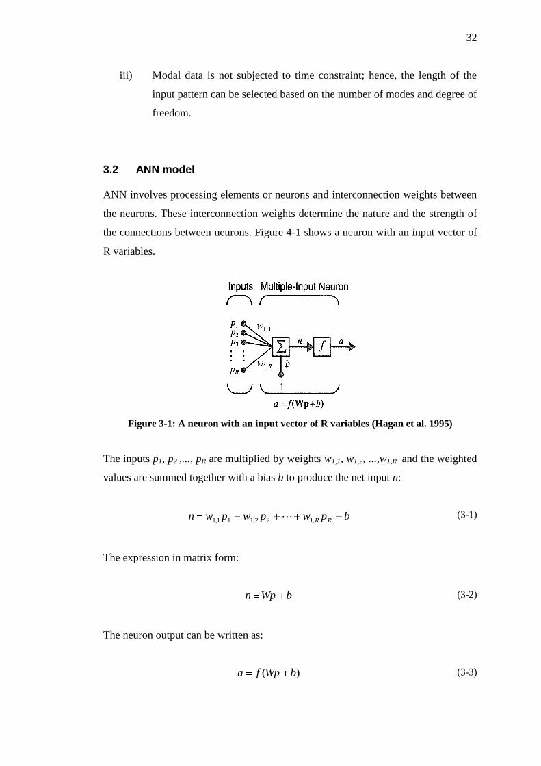
3.2 ANN MODEL ............................................................................................................................ 32
3.2.1 Selection of an ANN architecture ....................................................................................... 34
3.2.2 Training an ANN model ..................................................................................................... 35
3.3 NUMERICAL EXAMPLES ........................................................................................................... 38
3.3.1 Numerical example 1 – Concrete slab ................................................................................ 38
3.3.2 Numerical example 2 – Steel frame .................................................................................... 46
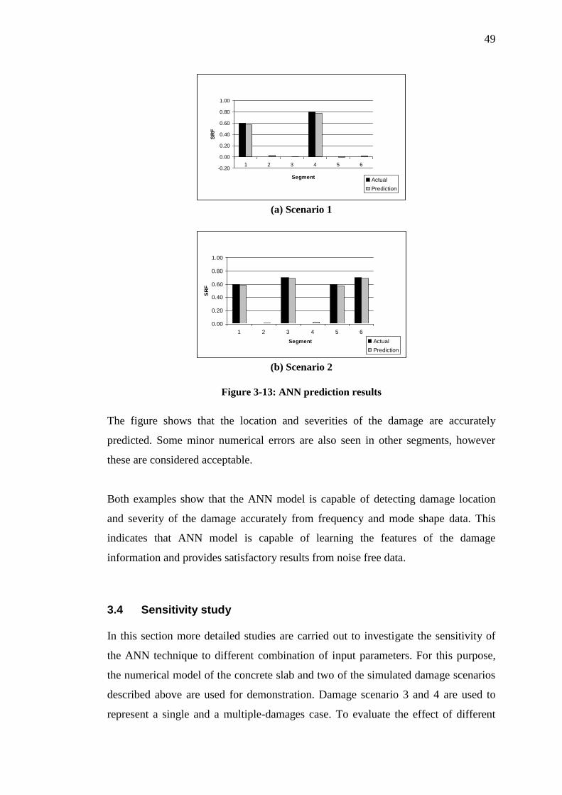
3.4 SENSITIVITY STUDY ................................................................................................................. 49
3.5 EXPERIMENTAL EXAMPLE ........................................................................................................ 55
3.6 SUMMARY ................................................................................................................................ 58
CHAPTER 4 ........................................................................................................ 59
4.1 INTRODUCTION ........................................................................................................................ 59
4.2 METHODOLOGY ....................................................................................................................... 61
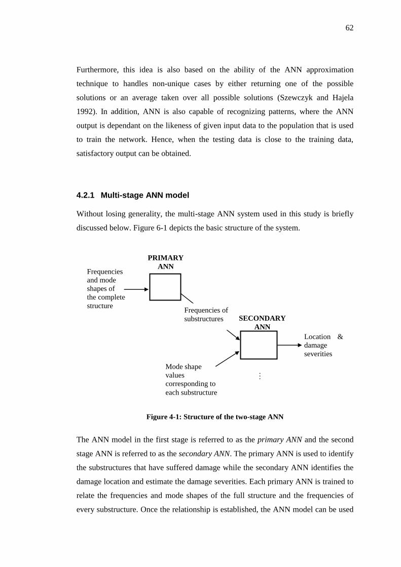
4.2.1 Multi-stage ANN model ...................................................................................................... 62
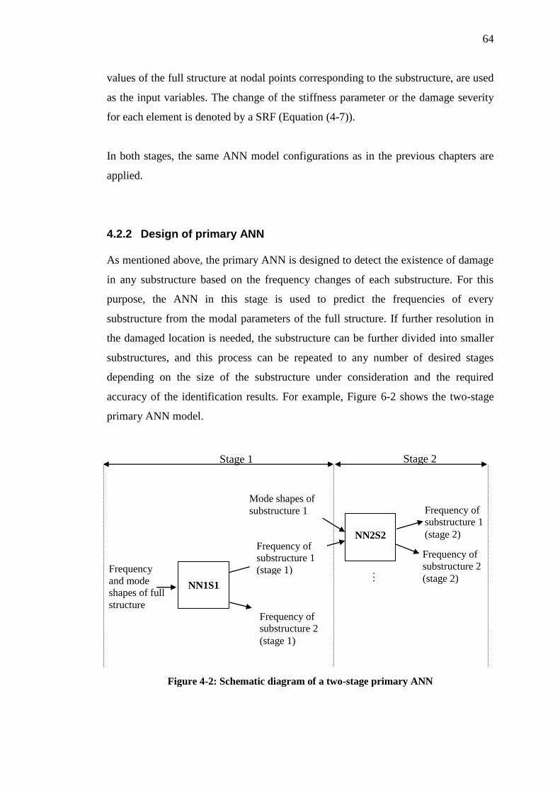
4.2.2 Design of primary ANN ...................................................................................................... 64
4.2.3 Design of secondary ANN .................................................................................................. 65
Page 6
iv
4.2.4 Training data ...................................................................................................................... 66
4.3 NUMERICAL EXAMPLE 1 – CONCRETE SLAB ............................................................................. 68
4.3.1 Conventional ANN .............................................................................................................. 70
4.3.2 Damage detection using multi-stage substructuring technique .......................................... 74
4.4 NUMERICAL EXAMPLE 2 – TWO-STOREY FRAME ...................................................................... 80
4.5 SENSITIVITY STUDY ................................................................................................................. 84
4.6 SUMMARY ................................................................................................................................ 90
CHAPTER 5 ........................................................................................................ 92
5.1 INTRODUCTION ........................................................................................................................ 92
5.2 METHODOLOGY ....................................................................................................................... 93
5.3 THE EFFECT OF UNCERTAINTIES ON DAMAGE DETECTABILITY WITH THE MULTI-STAGE ANN
METHOD ................................................................................................................................... 97
5.4 NUMERICAL EXAMPLE ........................................................................................................... 108
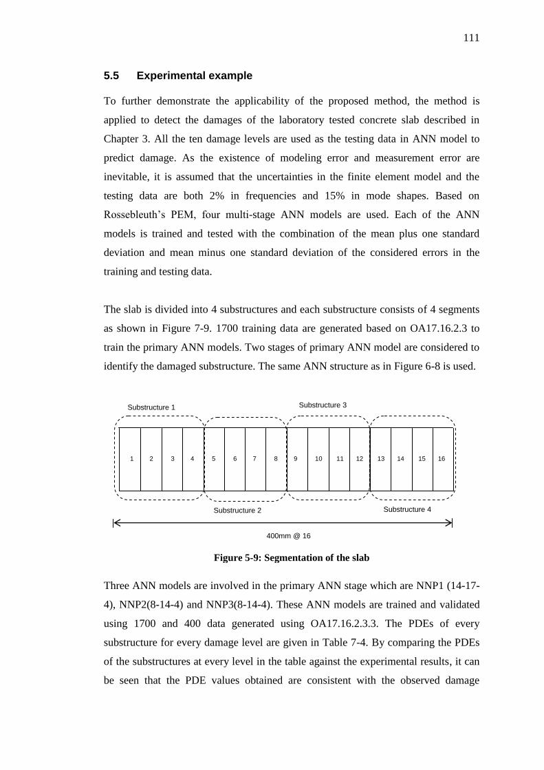
5.5 EXPERIMENTAL EXAMPLE ...................................................................................................... 111
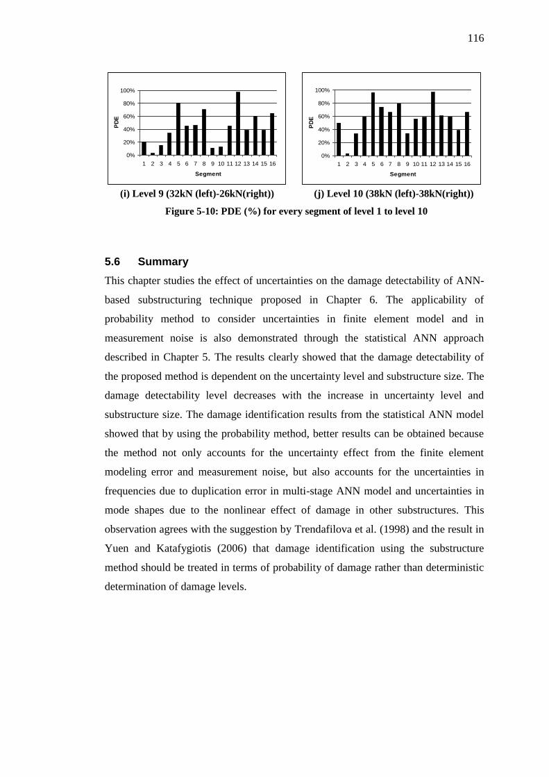
5.6 SUMMARY .............................................................................................................................. 116
CHAPTER 6 ...................................................................................................... 117
6.1 SUMMARY AND FINDINGS ...................................................................................................... 117
6.2 CONTRIBUTIONS .................................................................................................................... 118
6.3 RECOMMENDATIONS .............................................................................................................. 119
REFERENCES .................................................................................................. 121
Page 7
v
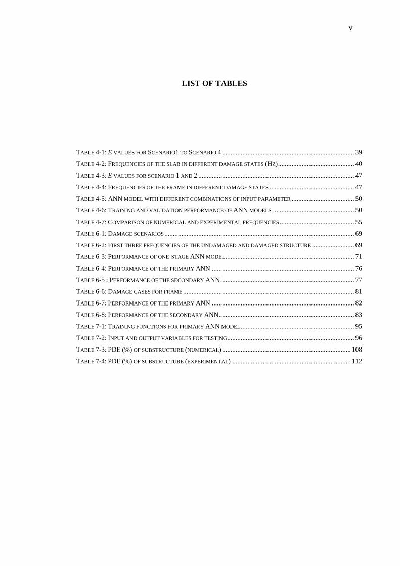
LIST OF TABLES
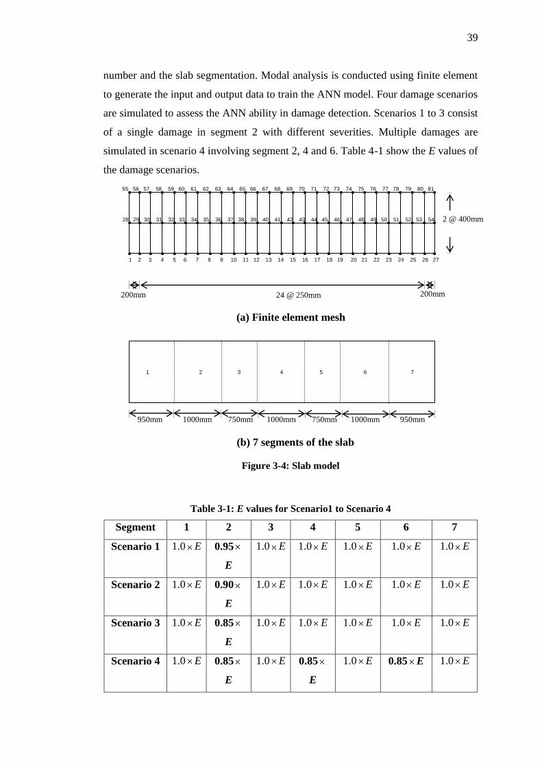
TABLE 4-1: E VALUES FOR SCENARIO1 TO SCENARIO 4 .............................................................................. 39
TABLE 4-2: FREQUENCIES OF THE SLAB IN DIFFERENT DAMAGE STATES (HZ) ............................................. 40
TABLE 4-3: E VALUES FOR SCENARIO 1 AND 2 ............................................................................................ 47
TABLE 4-4: FREQUENCIES OF THE FRAME IN DIFFERENT DAMAGE STATES .................................................. 47
TABLE 4-5: ANN MODEL WITH DIFFERENT COMBINATIONS OF INPUT PARAMETER ..................................... 50
TABLE 4-6: TRAINING AND VALIDATION PERFORMANCE OF ANN MODELS ................................................ 50
TABLE 4-7: COMPARISON OF NUMERICAL AND EXPERIMENTAL FREQUENCIES ............................................ 55
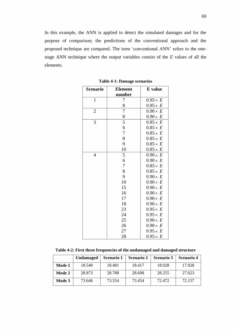
TABLE 6-1: DAMAGE SCENARIOS ................................................................................................................ 69
TABLE 6-2: FIRST THREE FREQUENCIES OF THE UNDAMAGED AND DAMAGED STRUCTURE ......................... 69
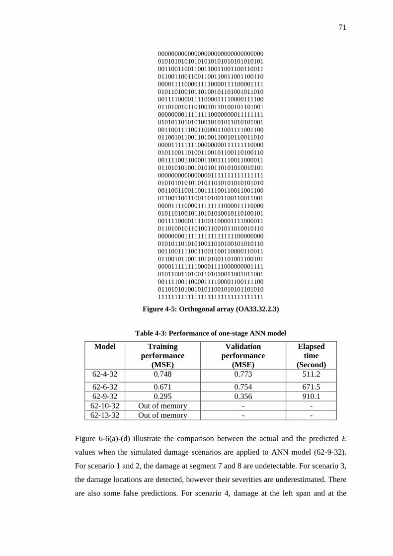
TABLE 6-3: PERFORMANCE OF ONE-STAGE ANN MODEL ............................................................................ 71
TABLE 6-4: PERFORMANCE OF THE PRIMARY ANN .................................................................................... 76
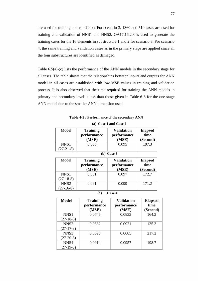
TABLE 6-5 : PERFORMANCE OF THE SECONDARY ANN ............................................................................... 77
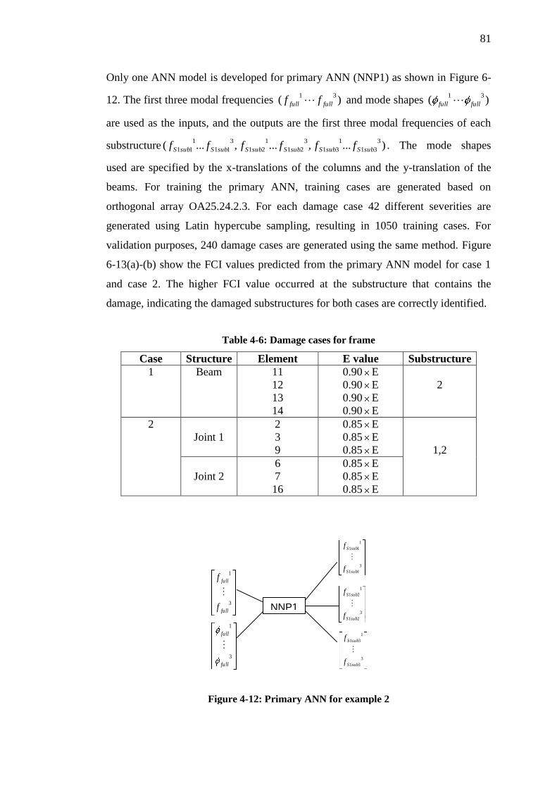
TABLE 6-6: DAMAGE CASES FOR FRAME ..................................................................................................... 81
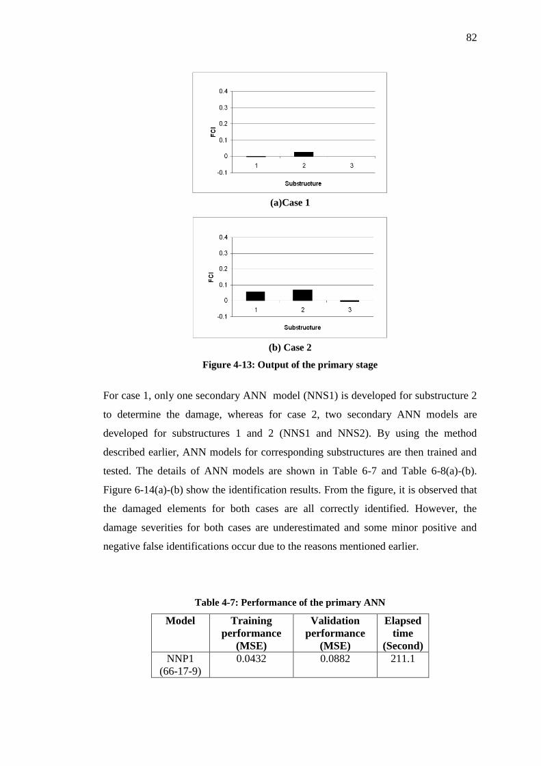
TABLE 6-7: PERFORMANCE OF THE PRIMARY ANN .................................................................................... 82
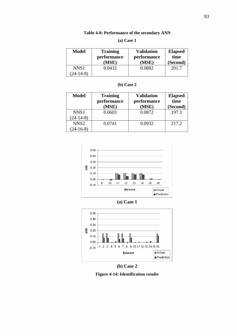
TABLE 6-8: PERFORMANCE OF THE SECONDARY ANN................................................................................ 83
TABLE 7-1: TRAINING FUNCTIONS FOR PRIMARY ANN MODEL ................................................................... 95
TABLE 7-2: INPUT AND OUTPUT VARIABLES FOR TESTING ........................................................................... 96
TABLE 7-3: PDE (%) OF SUBSTRUCTURE (NUMERICAL) ............................................................................ 108
TABLE 7-4: PDE (%) OF SUBSTRUCTURE (EXPERIMENTAL) ...................................................................... 112
Page 8
vi
LIST OF FIGURES
FIGURE 4-1: A NEURON WITH AN INPUT VECTOR OF R VARIABLES (HAGAN ET AL. 1995) ........................... 32
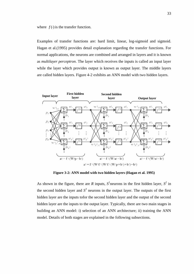
FIGURE 4-2: ANN MODEL WITH TWO HIDDEN LAYERS (HAGAN ET AL. 1995) ............................................. 33
FIGURE 4-3: HYPERBOLIC TANGENT SIGMOID FUNCTION (HAGAN ET AL. 1995) ......................................... 35
FIGURE 4-4: SLAB MODEL ........................................................................................................................... 39
FIGURE 4-5: THE FIRST FOUR MODE SHAPES IN DIFFERENT DAMAGE STATES. ............................................. 41
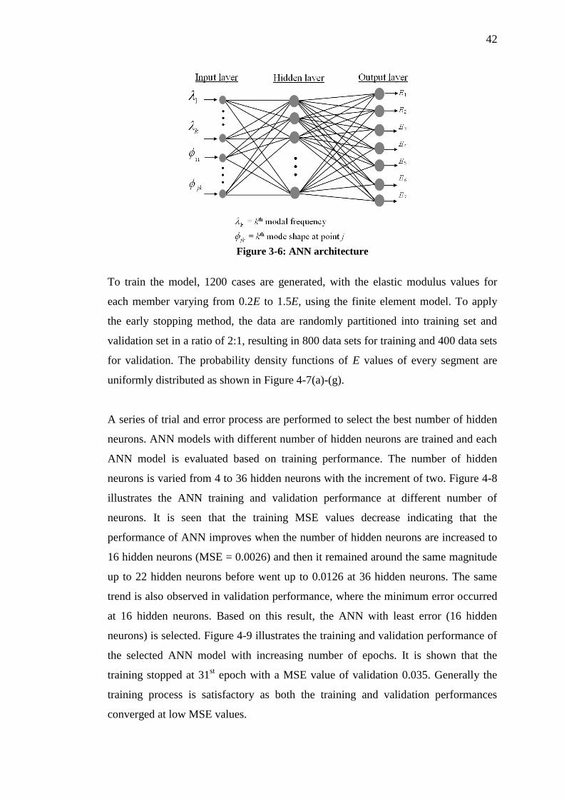
FIGURE 4-6: ANN ARCHITECTURE .............................................................................................................. 42
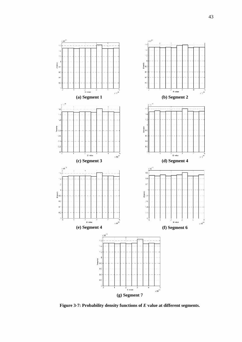
FIGURE 4-7: PROBABILITY DENSITY FUNCTIONS OF E VALUE AT DIFFERENT SEGMENTS. ............................ 43
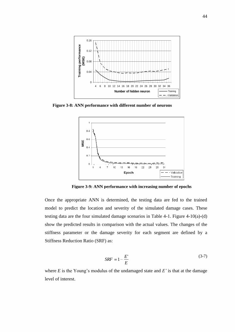
FIGURE 4-8: ANN PERFORMANCE WITH DIFFERENT NUMBER OF NEURONS ................................................. 44
FIGURE 4-9: ANN PERFORMANCE WITH INCREASING NUMBER OF EPOCHS ................................................. 44
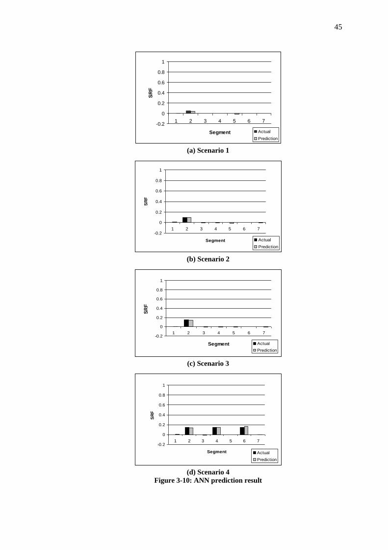
FIGURE 4-10: ANN PREDICTION RESULT ..................................................................................................... 45
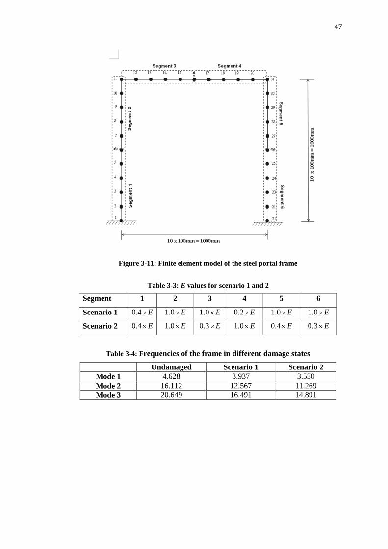
FIGURE 4-11: FINITE ELEMENT MODEL OF THE STEEL PORTAL FRAME ........................................................ 47
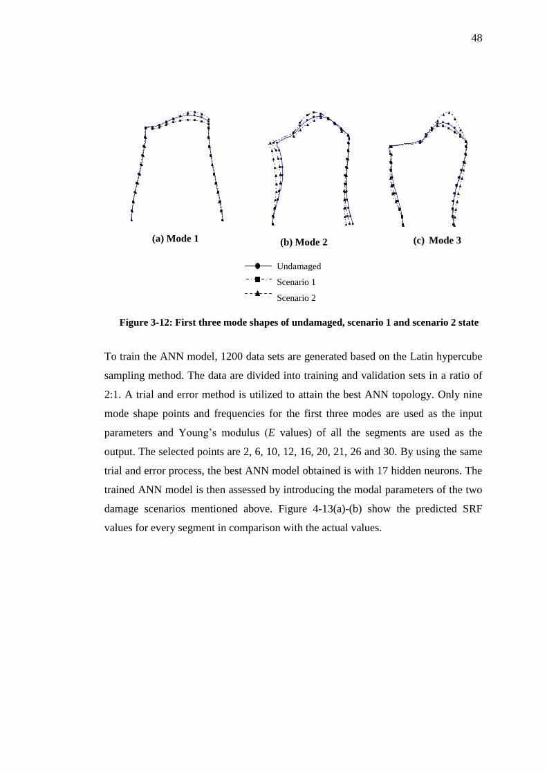
FIGURE 4-12: FIRST THREE MODE SHAPES OF UNDAMAGED, SCENARIO 1 AND SCENARIO 2 STATE .............. 48
FIGURE 4-13: ANN PREDICTION RESULTS ................................................................................................... 49
FIGURE 4-14: PREDICTION RESULTS OF MODEL 1 ........................................................................................ 51
FIGURE 4-15: PREDICTION RESULTS OF MODEL 2 ........................................................................................ 51
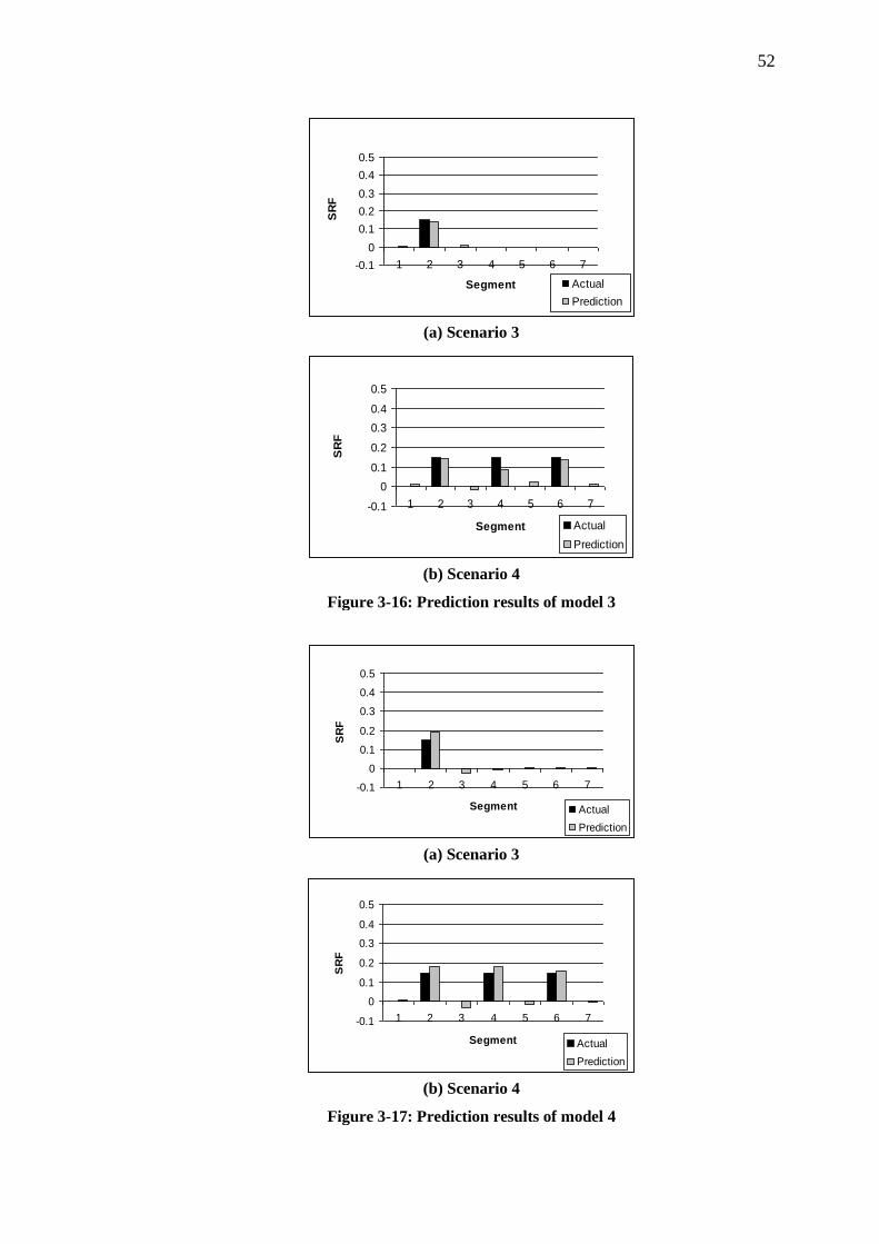
FIGURE 4-16: PREDICTION RESULTS OF MODEL 3 ........................................................................................ 52
FIGURE 4-17: PREDICTION RESULTS OF MODEL 4 ........................................................................................ 52
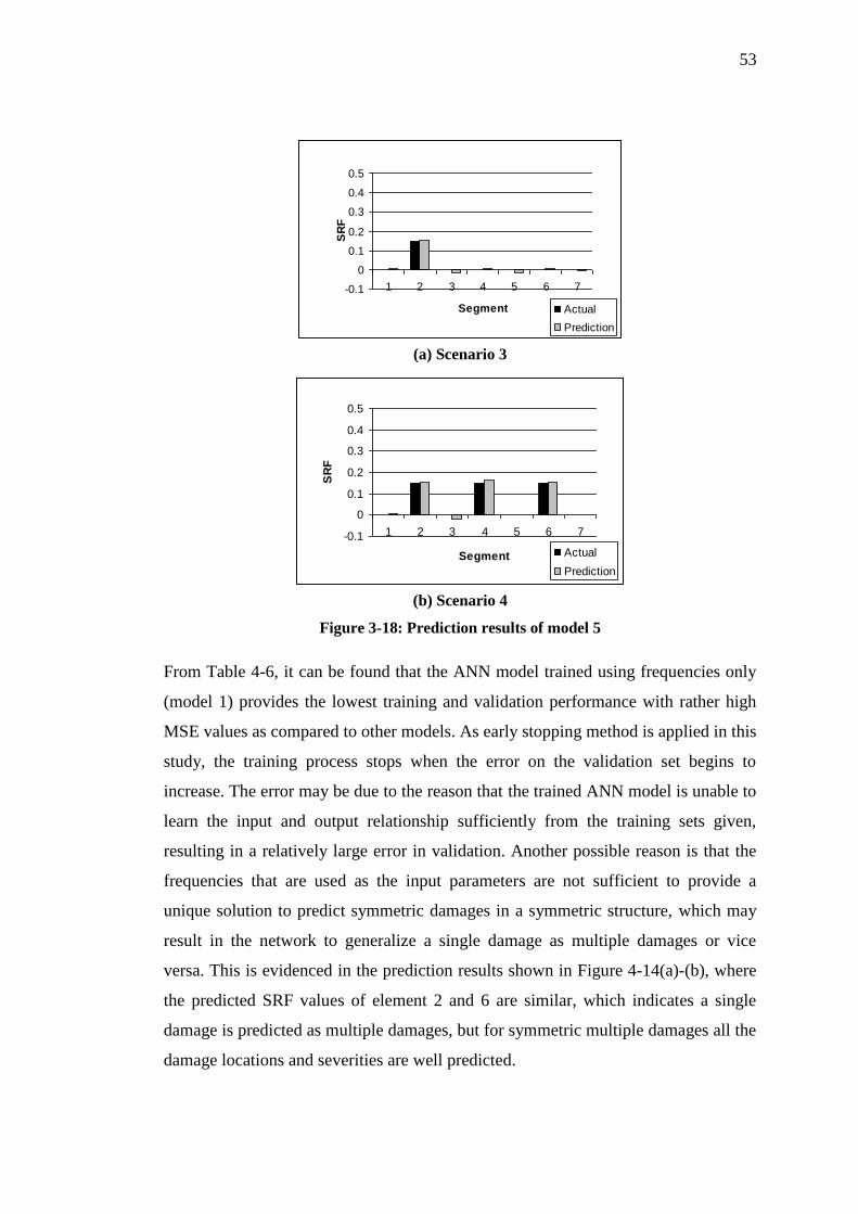
FIGURE 4-18: PREDICTION RESULTS OF MODEL 5 ........................................................................................ 53
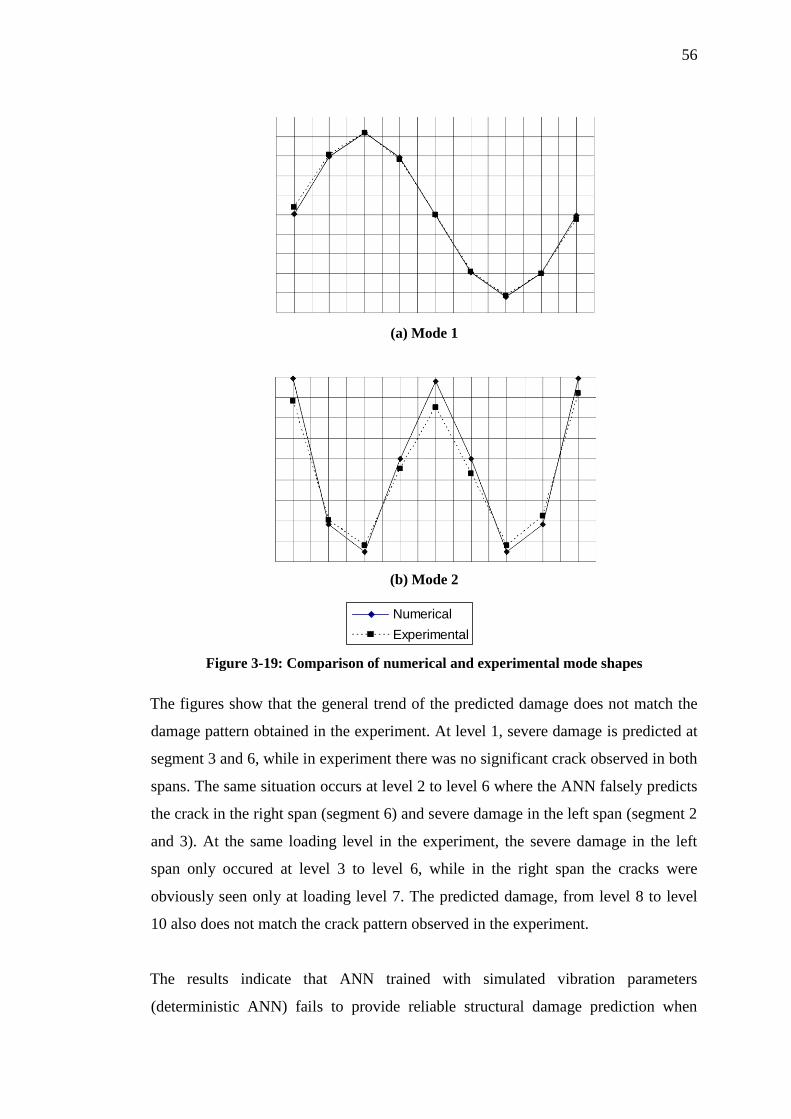
FIGURE 4-19: COMPARISON OF NUMERICAL AND EXPERIMENTAL MODE SHAPES ........................................ 56
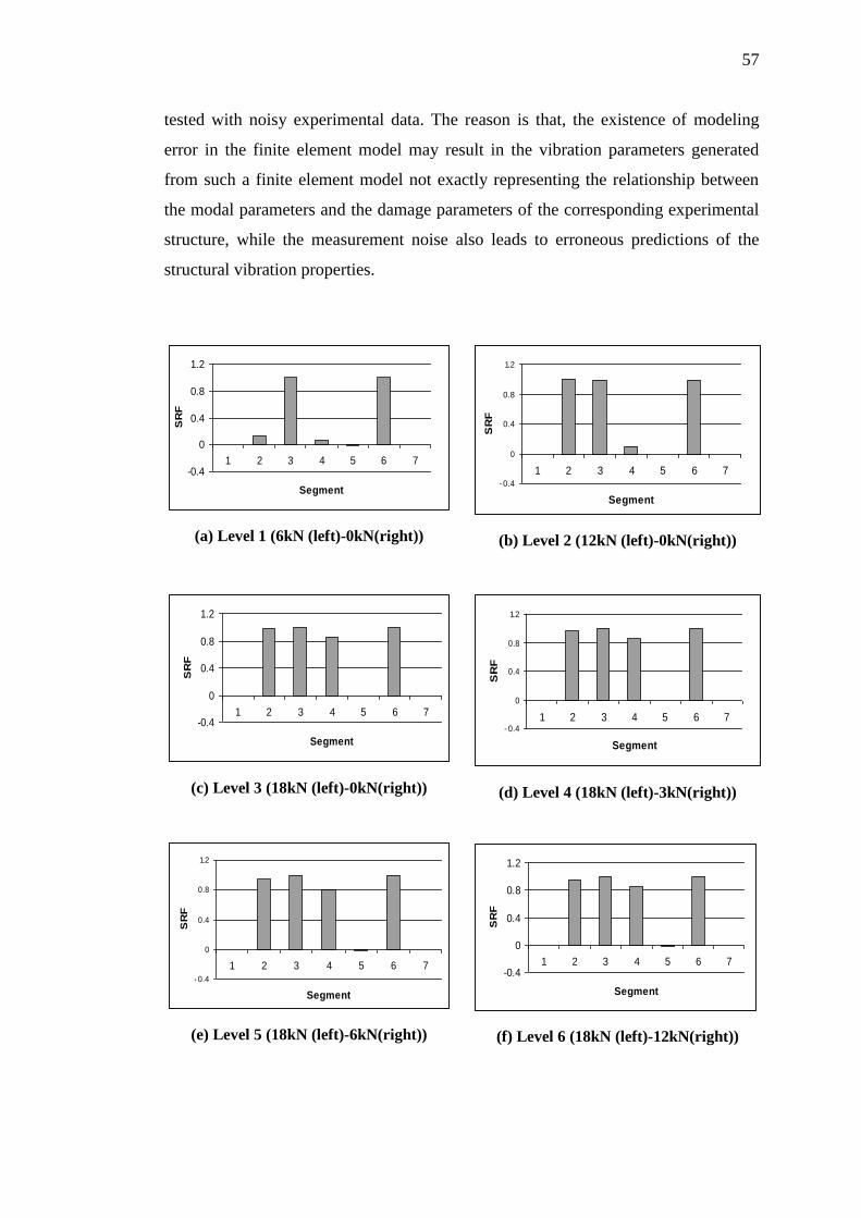
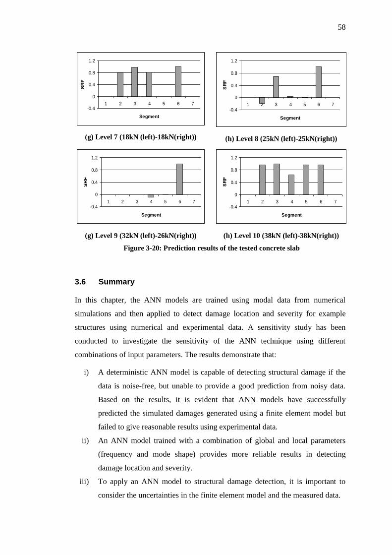
FIGURE 4-20: PREDICTION RESULTS OF THE TESTED CONCRETE SLAB ......................................................... 58
FIGURE 6-1: STRUCTURE OF THE TWO-STAGE ANN .................................................................................... 62
FIGURE 6-2: SCHEMATIC DIAGRAM OF A TWO-STAGE PRIMARY ANN ......................................................... 64
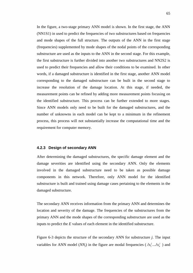
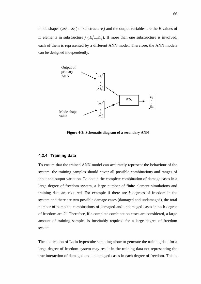
FIGURE 6-3: SCHEMATIC DIAGRAM OF A SECONDARY ANN ....................................................................... 66
FIGURE 6-4: SEGMENT OF THE SLAB ........................................................................................................... 68
FIGURE 6-5: ORTHOGONAL ARRAY (OA33.32.2.3) ..................................................................................... 71
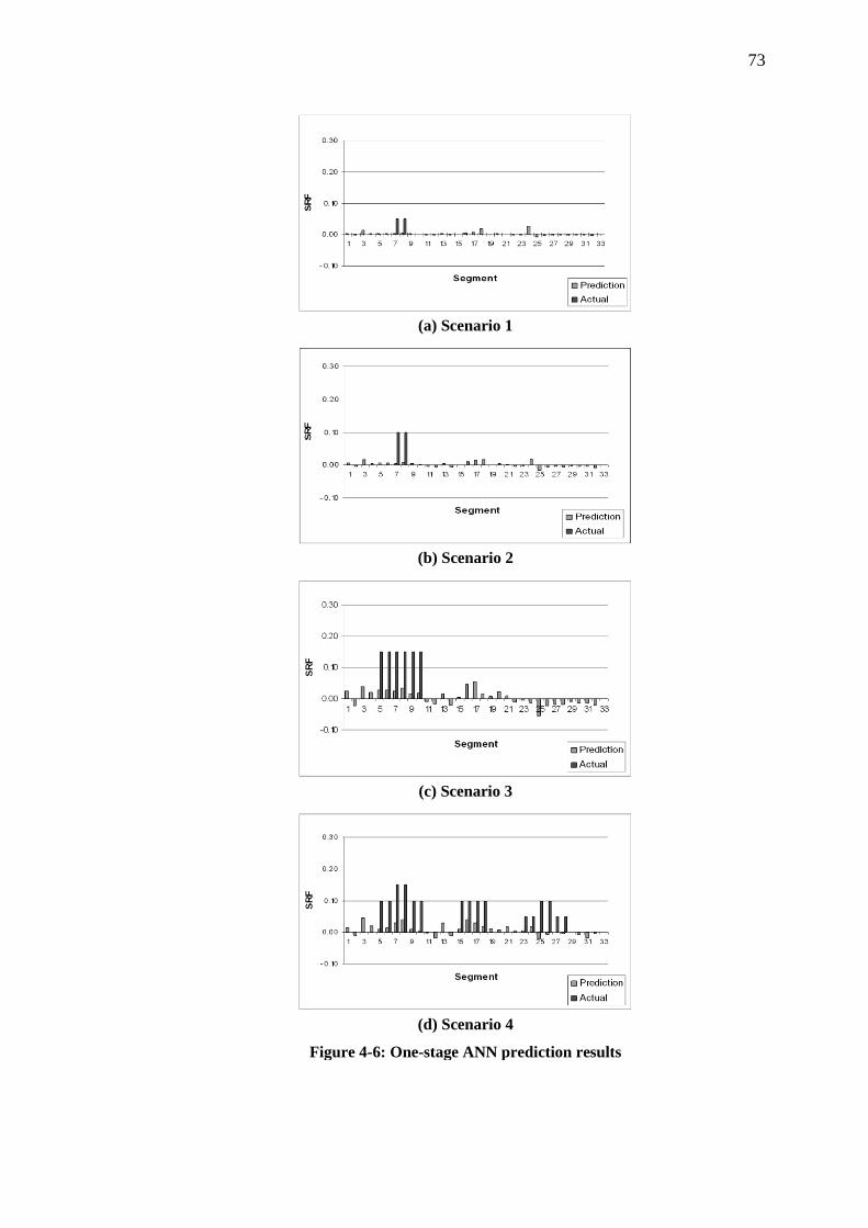
FIGURE 6-6: ONE-STAGE ANN PREDICTION RESULTS ................................................................................. 73
FIGURE 6-7: SUBSTRUCTURES OF THE SLAB ................................................................................................ 74
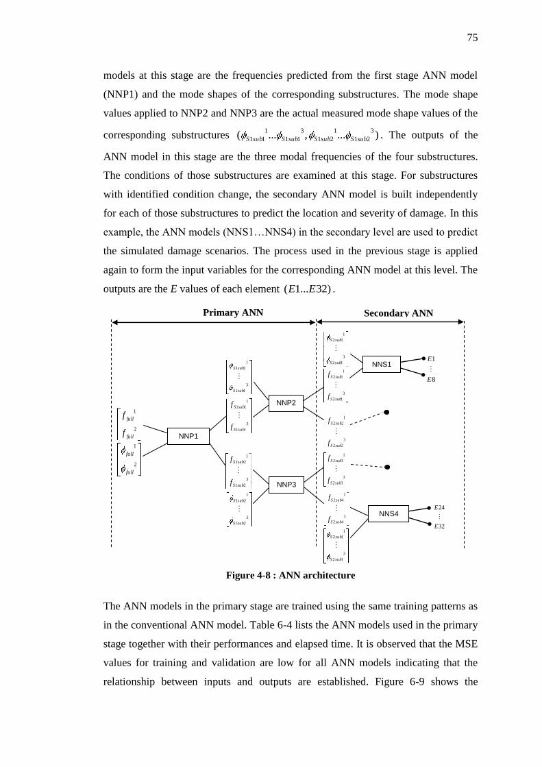
FIGURE 6-8 : ANN ARCHITECTURE ............................................................................................................. 75
FIGURE 6-9: OUTPUT OF PRIMARY ANN ..................................................................................................... 76
FIGURE 6-10: OUTPUT OF SECONDARY ANN .............................................................................................. 79
FIGURE 6-11: FINITE ELEMENT MODEL OF THE FRAME ................................................................................ 80
FIGURE 6-12: PRIMARY ANN FOR EXAMPLE 2 ............................................................................................ 81
Page 9
vii
FIGURE 6-13: OUTPUT OF THE PRIMARY STAGE .......................................................................................... 82
FIGURE 6-14: IDENTIFICATION RESULTS ..................................................................................................... 83
FIGURE 6-15: FINITE ELEMENT MODEL OF THE BEAMS ................................................................................ 84
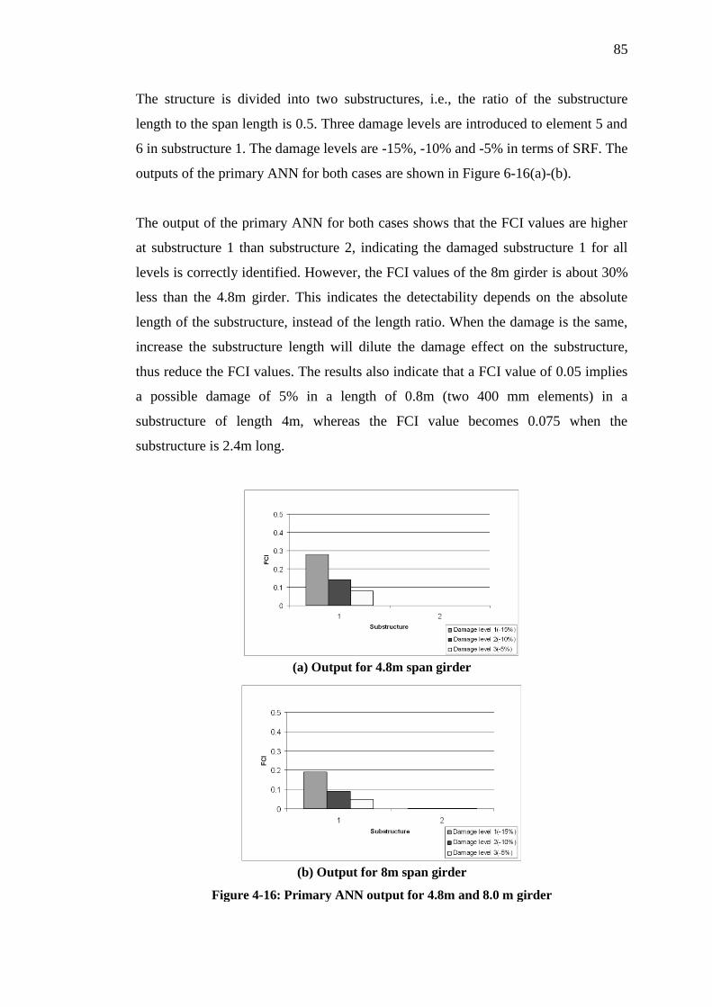
FIGURE 6-16: PRIMARY ANN OUTPUT FOR 4.8M AND 8.0 M GIRDER ........................................................... 85
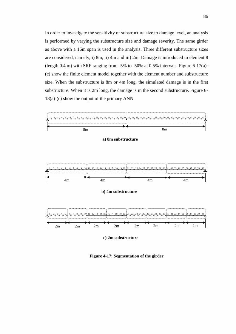
FIGURE 6-17: SEGMENTATION OF THE GIRDER ............................................................................................ 86
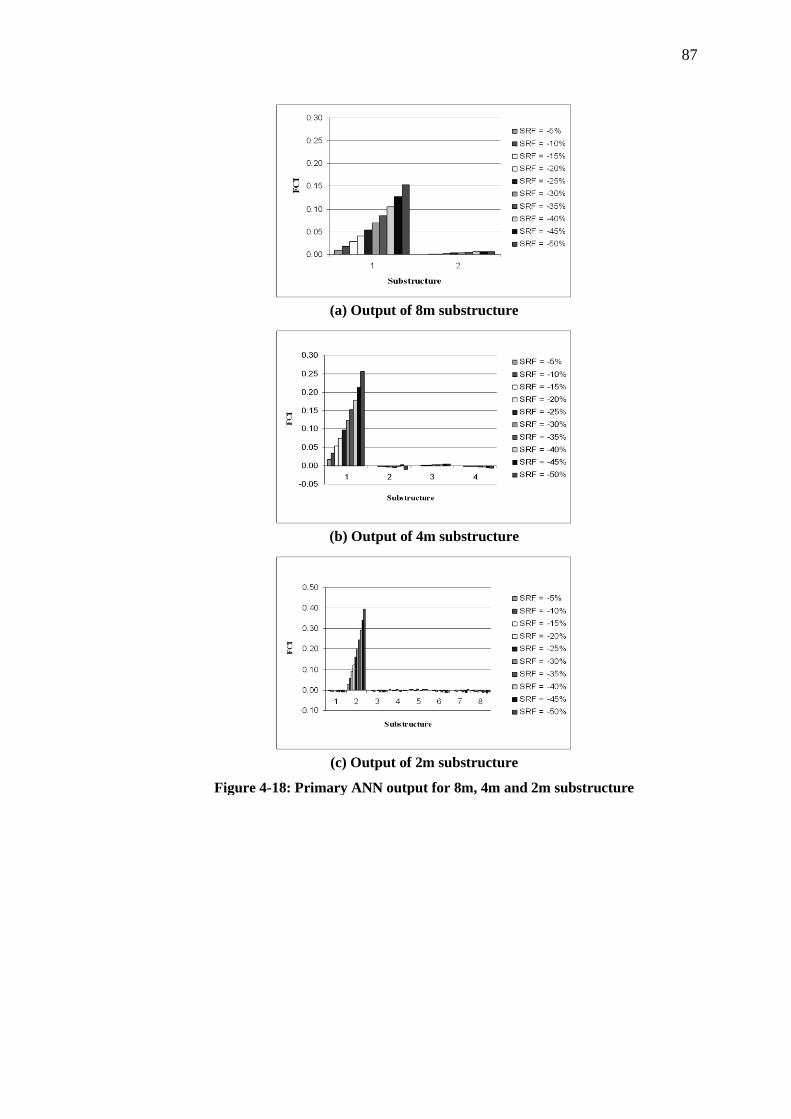
FIGURE 6-18: PRIMARY ANN OUTPUT FOR 8M, 4M AND 2M SUBSTRUCTURE .............................................. 87
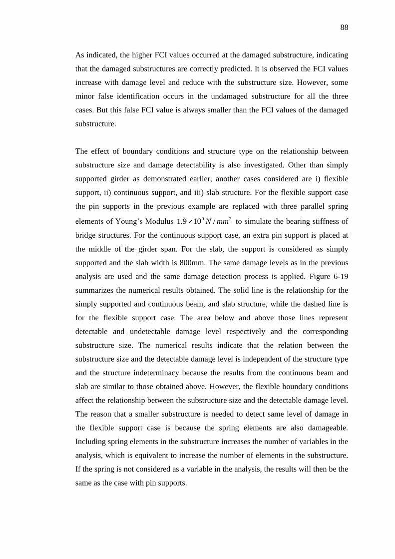
FIGURE 6-19: PRIMARY ANN OUTPUT FOR DIFFERENT STRUCTURE CONDITION ......................................... 89
FIGURE 6-20: DETECTABILITY OF DIFFERENT RATIOS OF DAMAGED ELEMENT SIZE TO SUBSTRUCTURE
SIZE ................................................................................................................................................... 90
FIGURE 7-1: PDE OF SIMPLY SUPPORTED GIRDER WITH 0.5% NOISE IN FREQUENCIES AND 5% NOISE IN
MODE SHAPES .................................................................................................................................... 99
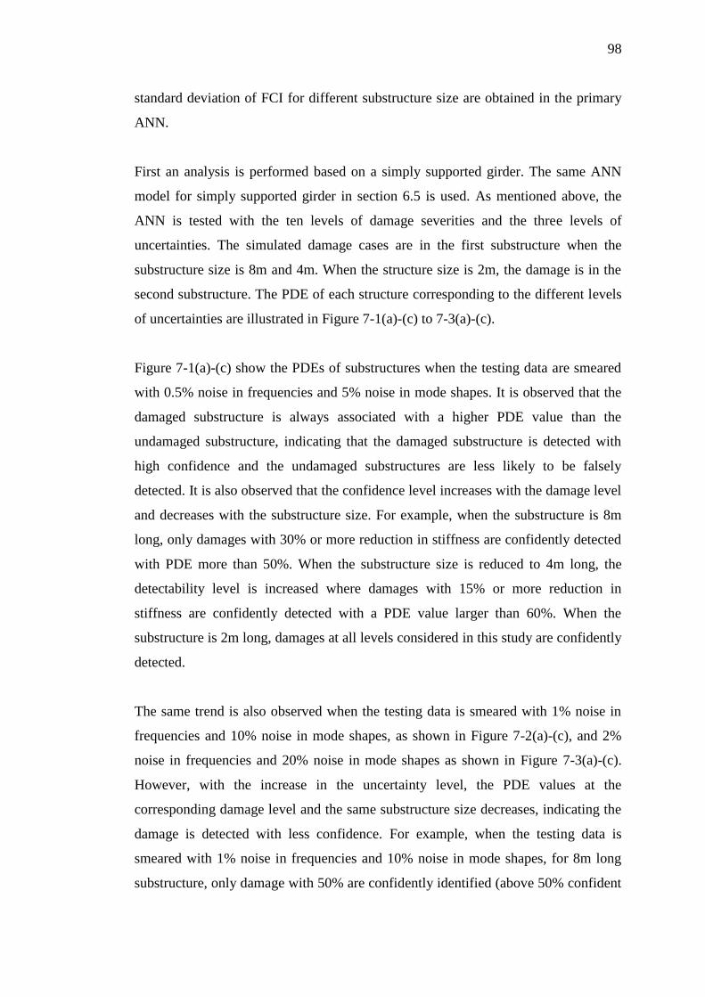
FIGURE 7-2: PDE OF SIMPLY SUPPORTED GIRDER WITH 1% NOISE IN FREQUENCIES AND 10% NOISE IN
MODE SHAPES .................................................................................................................................. 100
FIGURE 7-3: PDE OF SIMPLY SUPPORTED GIRDER WITH 2% NOISE IN FREQUENCIES AND 20% NOISE IN
MODE SHAPES .................................................................................................................................. 101
FIGURE 7-4: RESULTS OF THE SIMPLY SUPPORTED GIRDER ....................................................................... 103
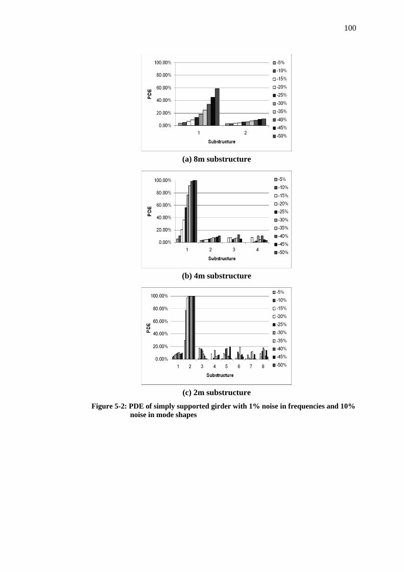
FIGURE 7-5: RESULTS OF THE FLEXIBLY SUPPORTED GIRDER .................................................................... 105
FIGURE 7-6: RESULTS OF THE CONTINUOUSLY SUPPORTED GIRDER .......................................................... 106
FIGURE 7-7: RESULTS OF THE SLAB STRUCTURE ....................................................................................... 107
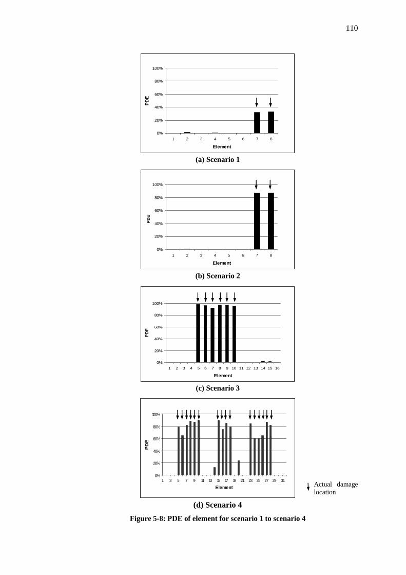
FIGURE 7-8: PDE OF ELEMENT FOR SCENARIO 1 TO SCENARIO 4 ............................................................... 110
FIGURE 7-9: SEGMENTATION OF THE SLAB ................................................................................................ 111
FIGURE 7-10: PDE (%) FOR EVERY SEGMENT OF LEVEL 1 TO LEVEL 10 .................................................... 116
Page 10
viii
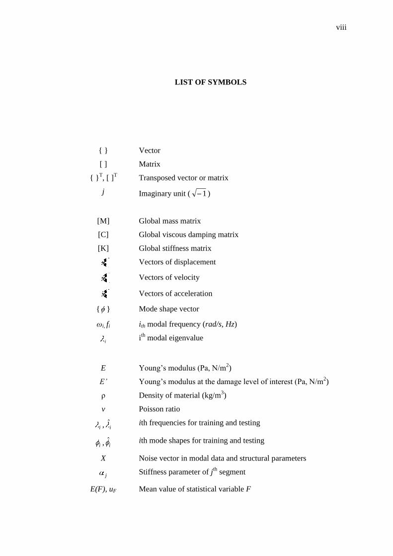
LIST OF SYMBOLS
{ } Vector
[ ]
Matrix
{ }T, [ ]
T Transposed vector or matrix
j Imaginary unit ( 1 )
[M] Global mass matrix
[C] Global viscous damping matrix
[K] Global stiffness matrix
x Vectors of displacement
x Vectors of velocity
x Vectors of acceleration
{ } Mode shape vector
ωi, fi ith modal frequency (rad/s, Hz)
i ith
modal eigenvalue
E Young’s modulus (Pa, N/m2)
E’ Young’s modulus at the damage level of interest (Pa, N/m2)
ρ Density of material (kg/m3)
v Poisson ratio
i , iˆ ith frequencies for training and testing
i , iˆ ith mode shapes for training and testing
X Noise vector in modal data and structural parameters
j Stiffness parameter of jth
segment
E(F), uF Mean value of statistical variable F
Page 11
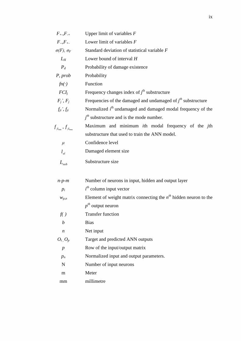
ix
F+-,F-+ Upper limit of variables F
F--,F+- Lower limit of variables F
σ(F), σF Standard deviation of statistical variable F
LH Lower bound of interval H
Pd Probability of damage existence
P, prob Probability
fn(·) Function
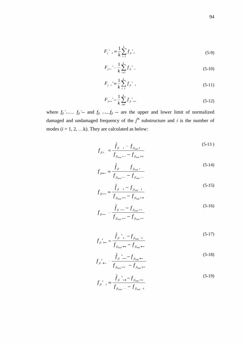
FCIj Frequency changes index of jth
substructure
Fj’, Fj Frequencies of the damaged and undamaged of jth
substructure
fji’, fji Normalized ith
undamaged and damaged modal frequency of the
jth
substructure and is the mode number.
minjif ,maxjif Maximum and minimum ith modal frequency of the jth
substructure that used to train the ANN model.
μ Confidence level
ell Damaged element size
subL Substructure size
n-p-m Number of neurons in input, hidden and output layer
pi ith
column input vector
wp,n Element of weight matrix connecting the nth
hidden neuron to the
pth
output neuron
f( ) Transfer function
b Bias
n Net input
Ot , Op Target and predicted ANN outputs
p Row of the input/output matrix
pn Normalized input and output parameters.
N Number of input neurons
m Meter
mm millimetre
Page 12
x
Abbreviation
ANN Artificial Neural Network
AAN Auto-associative Network
CDF Cumulative Distribution Function
COMAC Coordinate Modal Assurance Criteria
C.O.V. Coefficient of Variation
DFWNN Dynamic Time-Delay Fuzzy Wavelet Neural Network
DSD Dynamic Learning Rate Steepest Decent
DSM Damage Signature Matching
FABP Fuzzy Adaptive Backpropagation Algorithm
FRF Frequency Response Function
FCI Frequency Changes Index
GA Genetic Algorithm
ICA Independent component analysis
K-S test Kolmorogov-Smirnov goodness of fit test
MAC Modal Assurance Criteria
MSE Mean Squared Error
MDLAC Multiple Damage Location Assurance Criteria
NIL Noise Injection Learning
PDE Probability of Damage Existence
PDF Probability Density Function
SRF Stiffness Reduction Factor
TSD Tunable Steepest Descent
WNN Wavelet Neural Network
UFN Unsupervised Fuzzy Neural networks
Page 13
1
CHAPTER 1
INTRODUCTION
1.1 Introduction
Aging civil structures including bridges and buildings around the world are still in
service nowadays. Without careful monitoring and maintenance, these structures may
suffer severe damage or even collapse that may result in loss of human life and large
economic impact. Based on a study by Stidger (2006), in the United States, 24.5% of
bridges are classified as substandard and need rehabilitation. In Japan, the number of
aged bridges is expected to constitute half of all road bridges in year 2020 (Fujino
and Abe 2001). In Europe most of the bridges were built in 1960s, which now reach
their critical age and need rehabilitation. Engineers Australia also reported that the
overall quality of the national highway system is rated between averages to poor
condition (Engineers Australia 2005). There are many factors that can lead to
structure failure such as the usual weakening of material properties, the load
increments and unexpected event like extreme weather, earthquakes and vehicle
impact. In civil structures, damage can be denoted as cracking in the structure,
corrosion, deterioration of material properties or loss of prestressing. Many of these
defects are not visual and are not easy to identify in most cases.
There have been several disastrous incidents involving structural failures due to loss
of structural integrity such as the collapse of Mianus River Bridge in Connecticut in
1983 due to suspected corrosion of steel support members and fatigue loading, the
loss of entire fuselage section of Aloha Airlines Boeing 737 in 1988 due to fatigue
cracking. More recent incidents include the collapse of Kaoshiung-Pingtung bridge
in Taiwan in year 2000 injuring 20 people, the fell of a steel girder from an overpass
on Interstate 70 west of Denver in year 2004, crushing one car and killing three
people; and most recently in year 2007 in Minneapolis, an eight-lane highway bridge
collapsed into the Mississippi River. The incidents above indicate that structural
damage has become a crucial problem worldwide; therefore, more reliable and
effective damage identification methods are required.
Page 14
2
Current damage detection methods are categorized as: (1) local damage detection
method and (2) global damage identification method. Non-destructive testing (NDT)
methods have been used in local damage detection method, ranging from visual
inspection to more advanced methods such as X-rays, acoustic emission, ultrasonic
emission, eddy current and other wave propagation methods. However, the efficiency
of these approaches highly depends upon accessibility of the structural location and
individual expertise. Moreover, these methods require the area of the damage to be
known in advance and are very time consuming because they are only sensitive to a
small area as compared to the dimension of a civil structure. Therefore practitioner
and researchers demand for a global damage detection method that can determine the
damage existence, location and damage severity without relying on prior information
on the vicinity of the damage.
The majority of work to date in global damage identification methods has been
focused on the use of vibration properties to determine the damage existence,
location and severities. The theoretical basis for vibration based damage detection is
that the occurrence of damages or loss of integrity in a structural system causes
changes in the global vibration properties of the structure (e.g. natural frequencies,
mode shapes, damping, etc). Consequently, examination of structural response
characteristics provides useful information regarding the damage existence, location
and severity without prior knowledge of the damage states.
Vibration-based damage detection can be classified into model-based and non-model
based methods (James et al. 1997). Model-based damage detection methods locate
and quantify damage by correlating an analytical model with test data of the
damaged structure. Hence, it can provide quantitative information of damage as well
as damage location. These methods require finite element model and intensive
computation. Non-model based methods are very simple and straightforward, the
damaged structures are assessed by comparing the measurements of the damaged
structures and undamaged structures. However, the non-model based methods cannot
provide quantitative information of the structures, only location of the damage can be
determined.
Page 15
3
While there are many approaches that have been investigated and are still being
developed to identify damage from vibration properties, the approaches that do not
require detailed knowledge of the vulnerable parts or the failure modes of the
structure have an advantage to handle unexpected failure patterns. Moreover, the less
time consuming methods that provide less hurdles in design and implementation also
gain attentions. The Artificial Neural Network (ANN) method is one technique that
has been intensively studied.
Artificial Neural Networks (ANN) is a computational model inspired by the structure
and the information process capabilities of human brain. It is an assembly of large
number of highly interconnected simple processing unit (neurons). The ANN stores
knowledge in the form of connection strengths. These strengths are represented by
numerical values called weights which can be determined through a series of training
process.
ANN has been introduced to structural engineering since late 1980s. The
development of simple error backpropagation algorithm by Rumelhart (1986) has
boosted the research activities on its application in many areas including in structural
engineering. Since then, many papers have been published on its application to
structural engineering concentrating in structural analysis, design automation,
structural control and finite element mesh generation (Adeli 2001). In damage
detection, the ANN can be applied to identify the location and damage extent from
the measured dynamic responses. The early works in application of ANN in damage
detection began in 1990s and many studies concluded that the ANN model is a
promising tool for detecting damage in structures based on dynamic properties.
However, the majority of research in this area is limited to computer simulations and
small-scale laboratory tests. The practical application of these technologies to civil
engineering structures is still under research due to several reasons discussed below.
i) Civil structures have complicated geometry and consist of variety of
materials such as concrete, steel; rubber and asphalt, the inaccuracy in
estimation of strength and stiffness of materials and structure contribute
to uncertainties in modeling. Hence, producing an accurate finite element
model is very difficult. This may results in the vibration parameters
Page 16
4
generated from such a finite element model not exactly representing the
relationship between the modal parameters and the damage parameters of
the real structure. In other word, the ANN model may not be reliably
trained owing to finite element error. On the other hand, the existence of
measurement error in the measured data that is normally used as testing
data in an ANN model to detect damage is also unavoidable. Since the
reliability of an ANN prediction relies on the accuracy of the both
components, the existence of these uncertainties may result in false and
inaccurate ANN predictions.
ii) The effect of uncontrolled factors such as temperature, traffic loading and
humidity may induce significant amount of uncertainties in the captured
data and material properties, thus, will affect the reliability of damage
identification. For example an experimental study by Xia et al. (2006)
demonstrated that the changes of temperature and humidity cause changes
in natural frequencies of the structure. They also concluded that
temperature increase results in a reduction in the modulus of elasticity of
concrete significantly. Therefore, for reliable damage detection, the effect
of uncertainties should be considered for damage identification.
iii) ANN usually requires enormous computational effort especially when
structures with many degrees of freedom are involved. Due to this reason,
most applications of ANN for damage detection are limited to small
structures with limited number of degrees of freedom.
iv) The application of forced vibration test which is normally used for
damage identification is difficult for structures in service since it causes
service interruption. Application of ambient techniques are more suitable,
however this method usually is unable to reliably give higher modes,
which is more sensitive to small damage. Therefore, most of the damage
detection process in civil engineering would suffer from lack of data since
only a small number of measurement points and a few fundamental
modes are available.
Page 17
5
The aforementioned problems that would arise for damage detection for civil
structures provide the motivation of this study, which is intended to find solutions for
some of those problems.
1.2 Research objectives
The objectives of this study are:
i) To develop and demonstrate the applicability of damage detection using
ANN.
ii) To develop an ANN based probabilistic approach for damage detection
with consideration of the finite element modeling error and measurement
noise and to analyse the effect of these uncertainties on damage
identification result.
iii) To develop and demonstrate a substructure technique based ANN model
for damage detection of many degrees of freedom structures.
Page 18
6
CHAPTER 2
LITERATURE REVIEW
2.1 Introduction
During 1970s, engineers and researchers in offshore oil industries have made a
considerable effort to develop vibration based damage detection technique. The
objectives included the detection of near-failing drilling equipment and the
prevention of expensive oil pumps from becoming inoperable (Carden and Fanning
2004). The research in aerospace industry in vibration damage detection started in
the late 1970s and early 1980s. According to a review by Farrar et al.(2001), the civil
engineering community has studied vibration based damage detection since 1980s,
vibration properties such as frequency, mode shape and its derivatives have been
used for damage assessment focusing on bridge structures.
The vibration based damage detection is based on the equation of motion
0xKxCxM (2-1)
where M is the mass matrix, C is the viscous damping matrix, K is the
stiffness matrix. x , x and x are vectors of displacement, velocity and
acceleration; respectively.
The associated eigenvalue problem is
02
iii KCjM (2-2)
where i and i are the ith
modal circular frequency and mode shape respectively. j
is the imaginary unit
Page 19
7
If damage exists in a structure system, such as changes in the mass, stiffness or
damping or combination of them, the vibration characteristics such as natural
frequencies and mode shapes will change accordingly. Thus, damage can be detected
from changes of vibration properties which can be extracted from the measured
response data.
There are three basic types of data used in the vibration based damage detection.
They are time domain, frequency domain and modal domain. Time domain data is
the time history response of the structure that can be measured by sensors (e.g.
displacement, acceleration). This time series data can be converted to the frequency
domain using Fourier transform to form a frequency response function (FRF).
Further analysis of the frequency domain data is often undertaken to extract the
modal domain parameters such as vibration frequency, mode shape and damping.
While all the above data reflect the condition of a structure, damage identification
can be done based on data in the time, frequency or modal domain. However, there
are arguments about the suitability of data for damage detection since in each stage
the processing involves data compression process which results in a reduction in the
volume of the data. For example Banks et al. (1996) questioned the suitability of
modal data for damage detection arguing that modal data is a global system
properties while damage is a local phenomenon. In contrast, according to Friswell
and Penny (1997), the FRF and modal data essentially contain the same information
unless the modes are out of range. Lee and Shin (2002) pointed out that the modal
domain data can be contaminated by modal extraction error not present in the FRF
data. They suggest that FRF can provide more information as the modal data is
extracted from a very limited range around resonance. Doeblíng and co-workers
(1996) concluded in their report that there are disagreements among researchers
about the suitable parameters for damage identification. Research in all the three
domains are likely to continue because no constructive method has been found yet to
identify every type of damage in every type of structure. Nevertheless, most
applications of vibration based damage detection focused on the methods that are
based on the modal domain. This may be due to the fact that modal properties are
Page 20
8
easy to obtain and to interpret as compared to the more abstract features in the
frequency domain and the time domain.
Damage can be classified into linear or nonlinear. A linear damage is when the
initially linear-elastic structure remains linear-elastic after damage. The changes in
the modal characteristics are a result of changes in the geometry, boundary condition
or material properties of the structure. The structural response can still be modeled
using linear equations of motion. Nonlinear damage is defined as the case when the
initially linear-elastic structure behaves in nonlinear manner after the damage has
been introduced. One example of nonlinear damage is the formation of a crack that
subsequently opens and closes under the normal operating vibration environment.
The majority of the studies reported in the technical literature addresses only the
problem of linear damage detection (Farrar and Doebling 1997).
Rytter (1993) classified damage identification into four levels:
Level 1: Determination that damage is present in the structure
Level 2: Determination of the geometric location of the damage
Level 3: Quantification of the severity of the damage
Level 4: Prediction of remaining service life of the structure
Doebling et al. (1998) presented an extensive review on the damage detection
methods based on modal parameters and Carden and Fanning (2004) provides the
updated version. These literature reviews concentrated primarily on Level 1 to 3
only. Level 4 is generally associated with the fields of fracture mechanics, fatigue
life analysis, or structural design assessment which is rarely addressed by
researchers.
This section reviews various methods for damage detection based on vibration data,
emphasizing on structural engineering applications. Due to a vast amount of
publications in this area, the literature review in this section mainly focuses on the
technical papers published after 1990; however some earlier publications that are
considered to be important are also included. The damage identification methods
Page 21
9
reviewed below are categorised based on vibration parameters and analysis
techniques.
2.2 Artificial neural network methods
Most of the proposed methods in the literature above are a direct process involving
constructions of mathematical models, which are then used to develop a relationship
between damage conditions and changes in structural response. Since the damage
identification is an inverse process, where causes must be discerned from effects, a
search for the causes of the structural responses is quite complicated and
computationally expensive. A unique solution often does not exist for an inverse
problem, especially when insufficient data is available. Thus, it is very difficult to
evaluate an existing structure that has suffered some unknown type of damage using
traditional damage detection methods based on a priori knowledge of damage
scenarios. The model updating techniques which include iterative method and
optimization method also results in a huge amount of calculation and is time
consuming. Although many algorithms have been developed to improve the updating
process, it still remains computationally complex.
As ANNs are known for its capability to model nonlinear and complex relationship,
the inverse relationship between structural responses to structural characteristics can
be modeled.
The application of ANN to civil engineering began in 1989. The first journal article
on civil/structural engineering was published by Adeli and Yeh (1989) to solve a
problem in engineering design. Adeli (2001) has conducted a comprehensive review
in the application of ANN in civil engineering. In damage detection, Wu et al.(1992)
published the first journal article to detect damage from dynamic parameters by
employing ANN.
The basic strategy in applying ANN model for damage detection is to train the ANN
model to recognize the changes of structural characteristics based on measured
response. This is due to the reason that the rules governing the cause and effect
Page 22
10
relationships must be established explicitly and methodology for using these
relationships must be developed in priori (Wu et al. 1992). Through a training
process, ANN is able to extract the relationship between inputs and outputs and then
store within the connection strengths.
There are two main steps in building an ANN model, i) training stage; and ii) testing
stage. In training, a network is trained by data of various damage cases using an
appropriate training algorithm. In the testing stage, the trained ANN is fed with input
data that has not been used in the training. To generate a set of data that can be used
in training process, the data must contain the information regarding cause and effect
relationships. In any typical application of ANN, an appropriate ANN architecture
must be determined in the first place followed by selection of training algorithm to
train the network. In most cases ANN architecture is expressed as n-p-m, where
n,p,m are the number of neurons in input, hidden and output layer respectively.
In previous studies, many types of parameters corresponding to measured response
were applied as the inputs. For damage detection, measured response parameters
(time domain or frequency domain or modal domain data) are normally used as the
inputs, while for the outputs, the non-parametric and parametric parameters were
normally used to represent the condition of the structure. Non-parametric parameter
refers to any form of variable used to classify the structure condition, such as binary
number, while parametric parameters quantify the damage extent, such as reduction
of stiffness value (Xu et al. 2004). The application of ANN for damage detection is
the major concern in this study.
As the research in the application of ANN for damage detection progressing, in this
subsection, the related studies are reviewed in three major categories: i) Input and
output parameter; ii) process mapping and algorithm; and iii) application.
2.2.1 Input and output parameter
As mentioned earlier, the relationships between cause and effect are obtained from
training data through an appropriate training scheme. Most researchers in the early
Page 23
11
stage focused on determining the appropriate combination of input and output
variables.
The first journal article by Wu et al. (1992) applied FRF of acceleration data as the
input vector. The FRF between 0 and 20Hz was discretized at the interval of 0.1Hz
resulting in 200 spectral values. Binary number, 1 and 0 were used as the output to
represent the undamaged and damaged condition of each member in a simulated
three-storey building. Povich and Lim (1994) verified the application of FRF as the
input parameters to detect damage condition in a 20-bay planar truss composed of 60
struts. 394 input nodes were used, corresponding to spectral values between 0 and 50
Hz. The same binary code was applied as the outputs to represent the condition of
each strut. Both studies demonstrated that ANN is capable of learning the behaviour
of damaged and undamaged structures and to identify the damaged member from
patterns in the FRF of the structure.
Kudva et al. (1992) examined the viability of measured strain values at discrete
locations as the inputs to deduce the damage size and locations on a numerically
modeled plate stiffened by 4 x 4 array bays. ANN was used to relate the inputs with
the damage size and location of the damaged bays. Two output nodes were used; to
represent damage location and damage size. The results show that the training
performance is good which indicate that ANN is able to provide good correlation
between strain values and damage location and size. However, some false predictions
are experienced in testing, due to the reason that strain values is unable to provide
unique representation of damage location and severities. Furthermore, the output
nodes setting used in this study only allow ANN to detect single damage only.
Worden et al. (1993) applied the same approach to classify the damaged and
undamaged member of an experimental framework structure in terms of binary
number. The study suggested that ANN should be trained using noise-corrupted data
to produce better classification results if experimental data is employed.
Elkordy et al. (1992) used the percent changes in vibrational signatures obtained
from experimental study of a five-story frame as input to backpropagation ANN.
They demonstrated that using the percent changes in vibrational signatures rather
Page 24
12
than absolute values effectively distinguishes between the patterns corresponding to
different damage states. Pandey and Barai (1995) applied vertical displacements at
selected nodes as the input parameter to identify damage in a numerically modeled
21-bar bridge truss structure. The outputs are cross sectional area of every member.
The damage scenarios considered were formed by reducing the cross section of the
corresponding truss members. The ANN models used in this study were able to
predict the cross sectional area of the simulated damages with a minimum error
percentage.
A more detailed study related to the number of measurement nodes of vibration
signature was conducted in Barai and Pandey (1995). The vibration signature of a
bridge truss structure under moving load was used as the ANN’s input. The
prediction performance of ANN models employing single-node; three-node and five-
node of measurement were compared. The authors concluded that the vibration
signature obtained from single-node provides better performance compared to
multiple measurement nodes. However, the authors did not address the issue
regarding selection of time interval and length of vibration signature.
Masri et al.(1996) carried out a study regarding the effect of different lengths of
vibration signature to ANN performance. A backpropagation ANN model was
trained to detect the abnormality in a linear and nonlinear single-degree-of freedom
system based on vibration signature. The inputs of the network are the relative
displacement and relative velocity, and the output is the restoring force. The results
show that better training and prediction performances are obtained when longer
vibration signature is used as the input. This is aligned with the ANN learning theory
that more information provides the better prediction results. However, there was no
specific guideline provided on selecting the appropriate length of the vibration
signature. The application of this method to actual data was demonstrated in
Nakamura et al. (1998), while Masri et al.(2000) applied the proposed approach to
experimental nonlinear multi-degree of freedom system.
The use of time series data such as FRF and vibration signature required a small
sampling rate, in turn, a tremendous amount of training data is needed and a large
Page 25
13
training time may involve. In order to address this issue, researchers proposed
several alternatives.
In Spillman et al. (1993), instead of using spectral values, the authors applied the
amplitudes and frequencies of the first two modal peaks of Fourier transformed
acceleration time history signal together with impact intensity and location of the
sensor as inputs to ANN model. A 4.5m steel bridge element was used as an
example. Damage was introduced by cutting and bolting a plate reinforcement over
top of the cut. With the plate attached, the element was considered undamaged. With
the bolts loosened, the element was considered to be partially damaged. The impact
intensity and location were also used as inputs. An ANN model with 14 inputs, 20
hidden nodes and 3 outputs were used, one for each of the possible damage. The
results show that the proportion of correct diagnosis was around 60%. The authors
justified this number by citing the small size of the training data.
Islam and Craig (1994) applied natural frequency as the input parameters of ANN in
determining the location and size of delamination in a cantilever delaminated
composite beams. Numerical and experimental examples were used to verify the
proposed method. The ANN architecture consisted of three layers with five nodes in
the input layer corresponding to the first five modal frequencies. Three and two
nodes were used in hidden and output layers respectively. The nodes at the output
layer corresponding to delamination size and location. The ANN was trained with
14000 training patterns. Their results showed a good agreement between natural
frequency and damage location and size. The simulated and experimental damages
were successfully detected. Ceravolo and De Stefano (1995) also applied natural
frequency as the input to ANN model to predict the (x,y) coordinates corresponding
to the damage location. A truss structure simulated by finite element model was used
as the example. The damage was imposed by removing truss elements. A
backpropagation ANN model with 10 input corresponding to 10 modal frequencies,
10 hidden nodes and two output nodes corresponding to the x and y position was
used. Only single-damage cases were considered. The network was trained with 18
samples consisting of various single-damage cases. The ANN located the damages
well.
Page 26
14
Similar input parameters were applied by Ferregut et al.(1995) to detect damage in
numerically modeled aluminium cantilever beam. A backpropagation with 6 input
nodes, 17 hidden nodes and 11 output nodes was applied. The first output node in
output layer was for damage magnitude, while the other 10 were for damage
location. The ANN was trained with 240 pairs of input and output data. The damages
were simulated by reducing the width and depth of the corresponding element from
1% to 30%. The results show that only severe damages were identified. This may be
due to the reason that the natural frequency alone is not sensitive to small damage. A
similar outcome was experienced by Kirkegaard and Rytter (1994), when similar
input parameter was applied to identify damage in a 20-m steel lattice mast subject to
wind excitation. Damage was simulated by replacing lower diagonal with bolted
joints of diminished thickness. The ANN model was used to identify the mapping
from the first five modes of frequencies to the percentage of damages in member
stiffness. One output was used for each element of interest. The network was trained
with 21 examples generated from a finite element model. The results show that at
100% damage, the ANN was able to locate and quantify damage. At 50% damage
the ANN was able to predict the existence of damage but not the magnitude. The
damage less than 50% was not detected.
From the studies above, it is observed that natural frequencies alone are not effective
to identify damage in structures. Good results only limited to the cantilever structure
and single-damage only. As mentioned earlier, it is not capable in differentiating
damage in a symmetrical structure. Moreover, the frequency shift due to a small
damage is not significant, thus the frequency is not sensitive to small damages.
Elkordy et al. (1993) applied mode shapes as the inputs to ANN model to identify
damage in a five story building. The ANN model was trained using data generated
from finite element model and tested with numerical and experimental data. Two
types of ANN models were used. The two ANN models were trained using 11 and 9
training data respectively. The first model was used to classify the structure members
into damaged or undamaged, while the second was used to determine the percent
change in member stiffness. The output of the first and the second ANN model were
good when tested with numerical data but inaccurate results were observed when the
Page 27
15
experimental data was used. According to the authors, this may be because of the
inevitable measurement error in the measured data.
More comprehensive study regarding input parameter was conducted by Tsou and
Shen (1994). In their study, the detectability of two ANN model with different input
variables are compared. The first ANN model was trained using changes in
eigenvalues as the input parameters and the second ANN model was trained using a
combination of frequencies and mode shapes as the input vector. Those ANN were
tested with single and multiple damages. Instead of applying the conventional
classification method, a new ANN architecture was also proposed to deal with
parametric output parameter of multiple damages. Each node in the output layer was
used to represent the stiffness loses of each member. Finite element model of a three
degree of freedom and an eight degree of freedom spring system was used as the
examples. The authors concluded that the ANN with changes in eigenvalues as the
inputs was able to detect single and multiple damages in a simple system. However,
for more complicated problems, the information from mode shape is required to
provide more precise identification. The authors also claimed that by using modal
data as input parameters the length of the input vector was significantly reduced as
compared to FRF. Levin and Lieven (1998) verified the use of natural frequency and
mode shape as the input parameters to ANN model to update the finite element
model based on experiment modal data. A radial basis neural network was applied to
map the relationship between the vector and the structure properties. A simple ten-
element cantilever beam was used as an example. The successful applications of
natural frequency and mode shape as input parameter were also reported in other
studies.(Ko et al. 2002; Mehrjoo et al. 2007; Yun and Bahng 2000; Zapico et al.
2001).
A comparative study between static displacement and modal data as diagnostic
parameters for damage detection using ANN was conducted by Zhao et al. (1998). A
counterpropagation ANN was used to predict Young’s modulus of each structure
member. For static displacement, a numerical plane frame was used as an example.
Single and multiple damages were used for testing. The ANN was used to identify
the relationship between static displacement and Young’s modulus of each member.
The results show that ANN was not successful to detect multiple damages based on
Page 28
16
static displacement. For modal parameters, four different input parameters were
considered. i) natural frequencies; ii) mode shapes; iii) slope array; and iv) state
arrays. A three-span continuous beam was used as an example. The results show that
natural frequencies and slope arrays provide better results compared to mode shapes
and state arrays. The author concluded that the dynamics parameters are good
diagnostic parameters for damage detection, while static displacement is not suitable
to detect multiple damages as similar displacements can be obtained with different
combination of damage and loading.
Zang and Imregun (2001a) proposed a different method to reduce the size of FRF as
input variables. The authors employed a principal component analysis to reduce the
size of FRF before it can be used as the input variables. The output of the ANN
model is the condition of structure (healthy or damaged). The original FRF data of
railways wheels with 4096 data points in x, y and z direction was reduced to 7, 9 and
13 for x,y and z direction respectively. The reduced data sets were used as input
vectors to three different ANN models. 80 samples were used for training and 20
cases for testing. The results show that all the damage cases were correctly classified.
Zang and Imregun (2001b) quantified the above approach for slight damage
detection. Kim and Kapania (2006) enhanced the above method by applying
principal component together with orthogonal array method to reduce the number of
training data. According to Zang and Imregun (2001b) the application of FRF to
detect damage location and severities is still very difficult since a fine spatial
resolution of FRF is needed for damage location and the quality of raw FRF data
remains a major consideration.
Instead of using measured response parameters directly as the input variables to
ANN model, several researchers proposed proxy variables as the input parameters to
overcome the shortcomings of the existing method. Rhim and Lee (1995) highlighted
an issue regarding a large number of sensors needed if dynamic parameters are used
directly as the inputs. In their study, transfer functions of auto-regressive model with
exogenous input (ARX) served as the input patterns for damage classification using
backpropagation ANN. A Transfer functions was used as the system feature by
combining the information on a dynamic system from a given input-output data pair.
Page 29
17
The ANN was used to identify the map from characteristic polynomial to an
empirical damage scale. Each of the four outputs represented a different level of
damage, where 0 indicated no damage and 1 for total damage. The damage cases
were modeled as delamination in finite element model of a composite cantilever
beam. The authors chose ANN with 13 input nodes, 30 hidden nodes and 4 outputs
and trained with 10 training patterns. The ANN model was tested with three
examples and correctly identified the damage in those cases.
The development of wavelet-based approach for vibration data processing, which is
claimed to be more accurate, has enhanced the research in damage detection. Only
one paper found on the use of wavelet variables as the input parameters to ANN for
damage detection. Yam et al. (2003) applied structural damage feature proxy vectors
as the input to ANN to increase the sensitivity of the existing method to small and
incipient structural damage. Location and severity of the damage are used as the
output variables. The vectors were constructed based on energy variation of
structural vibration response. The vibration responses are decomposed into wavelet
sub-signals to extract structural damage information using wavelet packet analysis
method (WPA). By using a specified formula, the sub-signals are composed to form
a non-dimensional damage feature proxy vector. Numerical and experimental PVC
sandwich plates were used to verify the method. In numerical example, a damage
scenario with 12 cracks was modeled in the finite element model. A Backpropagation
ANN (32-16-4) was applied. 108 sets of training data were used for training. The
results show that the ANN was able to predict the crack location for all the 12 crack
cases. In experimental example, 6 crack cases with different length were considered.
Some errors in the results were observed in determining the crack length. This is
again because of the measurement error and modeling error.
Lam et al. (2006) proposed to use the changes of Ritz vectors as the features to
characterize the damage pattern defined by the corresponding locations and
severities. This approach is based on the reason that Ritz vectors possess higher
sensitivity to structural damage than natural frequency and mode shape. Ritz vectors
were extracted from frequencies and mode shapes using flexibility matrix. A Radial
basis function neural network was employed to identify the map between changes of
Page 30
18
Ritz vector and E values of any possible damage location. A numerically modeled
two-bay truss structure with 11 members was used to illustrate the proposed method.
ANN with 9 input neurons, 41 hidden nodes and 11 output nodes was used. Three
damage types were simulated for testing, ranging from single-damage to triple-
damage. The locations and damage severities for all cases were successfully
identified. The author concluded that the ANN trained with Ritz vector changes
provides more reliable results.
From the reviews above, the input parameters that used to identify damage with an
ANN model ranging from direct application of time domain data (e.g. vibration
signature), frequency domain (FRF) to modal domain data (frequency and mode
shape). Several attempts in using proxy parameters derived from dynamic data are
also reviewed. Despite of the fact that each vibration parameter has its own pros and
cons in damage identification as mentioned earlier, the application of time series data
(vibration signature and FRF) as the input parameter has another issue. In ANN
model, the values at each time interval are represented by an input node, thus for
time series data, a large number of nodes at the ANN’s input layer are needed. This
leads to a phenomenon known as ‘curse of dimensionality ‘ as discussed by Bishop
(1995) which significantly jeopardizes the efficiency and accuracy of ANN training
process. The modal frequency has the advantage of ease and accuracy of
measurement, since it is a global properties and not spatially specific, extra
information, such as mode shape can be used together to identify damage. Since
these parameters are not a time-based parameter, the number of ANN input node
depends on the number of modes and measurement points only, hence the length of
the input variables can be substantially reduced.
Application of wavelet data as the input variables provides an alternative for damage
detection, nevertheless there are many types of wavelets and there is no systematic
method to choose the most appropriate wavelet transform data for damage detection
(Marwala 2000).
It is important that the output of ANN is able to provide as much information as
possible about the damage status. In the early stage, most researchers applied non-
Page 31
19
parametric parameter as the outputs. This type of output parameter classified the
structure conditions to damaged and undamaged condition, thus the results are
limited to level 1 in Rytter’s terminology. Attempts to use parametric parameters as
the outputs are subjected to small structure system only. This may be due to
computational power that limits the training of large dimension ANN model, because
certain training algorithms require high computer memory to train the ANN model.
For example, Levenberg-Marquardt algorithm requires high computational power,
but in many cases it converges while the other algorithms such as conjugate gradient
and variable learning rate algorithm may not converge (Hagan and Menhaj 1994). As
a result, in most studies, only minimum number of output node is used at the ANN
output layer. This leads the researchers to use the coding system such as binary code
as the output to represent different structural location and condition. This limitation
also induces the difficulty in detecting multiple damages. As technology grows, more
studies used parametric parameters, involving structural parameters (e.g. damage
location and severity) as the outputs, thus qualitative way of damage detection have
taken place, and better information can be obtained.
2.2.2 Process mapping and training algorithm
Among various types of ANN models, multi-layer neural networks with
backpropagation algorithm are most commonly used in damage detection (Elkordy et
al. 1993; Elkordy et al. 1994; Povich and Lim 1994; Spillman et al. 1993; Wu et al.
1992). Although this ANN model has been proven to be an effective tool in damage
detection, it still suffers several drawbacks such as slow convergence and the
possibility to be trapped into local minima especially when it involves time series
input parameters. In this subsection, studies pertaining to various methods in
improving the conventional ANN model for damage identification are reviewed. This
includes the improvement of ANN performance in terms of mapping topology,
training algorithm and ANN integrated approach.
Szewczyk and Hajela (1994) introduced a new algorithm called Feature-sensitive
Neural Network to overcome the problem in variation of static displacements under
different load conditions. According to the authors, the feature-sensitive neural
Page 32
20
network is a modified version of counterpropagation neural network, which features
increased processing power over standard ANN while preserving its general
characteristics. This was done by implementing a clustering device as the hidden
layer to classify the input pattern on the basis of minimum disturbance principle. As
a result, only the weight vector of one neuron (the closest to a current input) is
modified. At the output layer, a nonlinear interpolation scheme was introduced to
increase the prediction accuracy. This new algorithm was applied on three numerical
structures of increasing complexity: a 2-dimensional six-bar truss, 2-dimensional 18-
degree of freedom portal frame and 3-dimensional 12-degree of freedom system. The
networks were trained with 200, 3600 and 3000 examples respectively. Quite
satisfactory results were exhibited for simple structure, but poor results were
observed for complex structures.
Ceravolo et al. (1995) extended the standard process mapping by applying
hierarchical ANN to detect the presence of structural faults. The network consists of
two levels of ANN model. The first level was used to determine the damaged area,
and the second level identified the damaged element in the area. Acceleration cross-
correlation values recorded over 1 second, with sampling period 0.005 second were
used as the inputs to backpropagation ANN model at both levels. Both networks
were trained with 54 and 18 training samples. A 5m numerically modeled beam was
served as the example. Although all the 12 simulated single-damage cases were
successfully detected, this approach is limited to single-damage cases only.
Worden (1997) applied novelty detection method using Auto-associative network
(AAN) in simple 3-degree of freedom simulated lumped-parameter mechanical
system. The purpose of the approach is to identify any changes in the system. The
AAN was forced to reproduce the patterns which were presented at the input layer.
The novelty index, which was defined as Euclidean distance between undamaged
and damaged pattern was used as the indicator of abnormality. The input and output
of the AAN was 50 spaced points of FRF between 0 to 50Hz. The effect of
measurement error was also considered by applying normally distributed noise in the
inputs. 50%, 10% and 1% fault cases were simulated by reducing the stiffness of one
of the spring in the system. The results showed that the AAN was able to detect the
Page 33
21
abnormality for 50% and 10% cases, but had difficulties to detect abnormality in 1%
damaged case. The author also demonstrated that the reliability of the proposed
approach also decreased as the noise increased. This method was only limited to
damage detection of level 1 in Rytters terminology.
Hung and Kao (2002) upgraded the novel detection method proposed by Worden
(1997) to comply with level 2 detection in Rytter’s terminology. Another ANN
model was introduced in the second stage to determine the location and severity. The
novel ANN model in the first stage was used to identify the undamaged and damaged
states of a structural system. The relative displacement, velocity and acceleration
were used as the input and output for the ANN in this stage. The partial derivatives
of the outputs of ANN in the first stage were used as the input for the ANN in the
second stage to determine the damage locations and severities. Examples of a single
degree-of freedom system and a multiple degrees-of freedom system were used to
demonstrate the approach. Simulated cases for both systems were satisfactorily
diagnosed. Kao and Hung (2003) further demonstrated the above approach using free
vibration responses.
Xu et al. (2004) proposed a new strategy of novel detection method to identify
damage directly from the vibration time-domain responses. The authors also claimed
that the proposed method is feasible to identify stiffness and damping without the
parameters of an undamaged structure to be known as a priori. Two ANN models
were applied. The first ANN model was used to model the time-domain behaviour of
a reference structure and the second was to identify the parameter of the structure.
Velocity and displacement and excitation force at the k time step were used as the
inputs and the outputs were velocity and displacement at the k+1 time step. The
deviation of the outputs from reference values indicates damage existence. The error
between the reference and the output values was then applied as the input for the
second ANN model to predict the parameters of the structure. A numerical five-story
frame was used as an example. The results showed that the stiffness parameters were
predicted with less than 7% error.
Page 34
22
In Marwala and Hunt (1999), a new mapping topology called committee neural
network to combine the information from FRF and modal data were proposed. Two
backpropagation ANN models were used to predict the fault identity based on FRF
and modal data respectively. Frequency energy calculated from FRF was used as the
input for the first ANN model and modal properties for the second. The predicted
fault identity values were combined to represent the condition of the structure. In this
study, a simulated 1.0m cantilever beam was used to illustrate the method. The beam
was divided into 5 segments, and the committee ANN was used to identify the
damage existence in each segment. An ANN architecture of 50-25-5 was selected for
the first ANN model and for the second one 55-25-5 was applied. 243 data were used
for training both networks. The results showed that those ANN was trainable with
low mean errors but no testing has been demonstrated. Marwala (2000) enhanced the
above study by applying wavelet transform data together with FRF and modal
properties. An experimental data of ten steel seam-welded cylindrical shells was used
for verification. The author claimed that the performance of the proposed approach is
not influenced by error and the effectiveness of the method is enhanced when
experimental data are applied.
Chang et al.(2000) proposed a modified backpropagation ANN algorithm known as
iterative artificial neural network to increase the ANN prediction accuracy in damage
detection based on modal data. The outputs of the trained ANN are fed to finite
element model to calculate the dynamic characteristics. If the calculated
characteristics deviate from the measured ones, the ANN model would go through a
retraining process. Natural frequencies and changes of mode shape curvatures were
used as the inputs, while structural stiffness was used as the outputs. A numerical
model and an experimental clamped-clamped reinforced concrete T beam were used
as the example. The results showed that all four simulated damage cases were
successfully detected; however, some slight errors were observed when experimental
data was used. According to the authors, this may be due to uncertainties related to
material properties or material in homogeneity.
Attempts to improve the performance of conventional backpropagation ANN
algorithm demonstrated in several studies above have shown promising results,
Page 35
23
however the computational efficiency is still an issue. Luo and Hanagud (1997)
proposed a dynamic learning rate steepest decent (DSD) algorithm to speed up the
training time. The DSD was used to train a neural network for direct identification of
composite structural damage through structural dynamic responses. Through
numerical experiments, the proposed method was shown to have much better
learning ability than the standard constant learning rate steepest descent method and
the accelerated steepest descendent method. The same approach was further
demonstrated by Zhu et al. (2002).
Xu et al. (2000) improved the above algorithm by introducing the concept of
dynamically adjusted learning rate and additional jump factor to speed up the
convergence of multilayer neural network. According to the authors the proposed
algorithm is able to alleviate the oscillation and stagnation in backpropagation
algorithm, thus speed up the convergence of the ANN model. In that study, the ANN
model was used to identify the correlation between the displacement response and
the location/size of the cracks. A numerically modeled anisotropic laminated plate
was used as the example. The authors claimed that the proposed algorithm can speed
up the convergence of neural network.
Liang and Feng (2001) argued the efficiency of dynamically adjusted learning rate
algorithms since this method heavily depends on selection of control parameters such
as error rate controller and learning rate controller that are typically determined
based on trial and error. Thus, the authors proposed a fuzzy adaptive
backpropagation (FABP) algorithm by integrating fuzzy logic concept with the
characteristics of ANN to identify the restoring forces in a nonlinear vibration
system. By applying fuzzy concept, error function and the changes of learning rate
are defined fuzzily based on human expertise. The authors concluded that FABP is
able to increase the training speed of the network. Nevertheless, this method has its
own limitation. The design of fuzzy logic approach still requires a rule based
formulation which is very difficult to implement and also time consuming. To tackle
this problem, Fang et al.(2005) developed a tunable steepest descent (TSD) algorithm
which is based on DSD algorithm incorporated with heuristics approach to improve
the ANN training process. According to the authors, a heuristic rule in which the
Page 36
24
learning rate is kept as large as possible to the extent that the network can learn
without increasing the error is used to determine the step size. This algorithm was
used to train ANN to establish relationship between FRF and damage
location/severity of a 20-elements cantilever beam. Key spectral points around the
resonant frequencies in FRF data together with 78 points of stiffness loss were
chosen as the input. The outputs were the stiffness loss of five specified locations of
the beam. The results show that ANN trained with TSD algorithm was able to detect
single and multiple damages. A comparison of training performance of the proposed
method with DSD and FABP was also performed. The authors concluded that TSD
algorithm outperforms DSD and FABP in training effectiveness without increasing
the algorithm complexity.
Another strategy to improve the performance of the conventional backpropagation
ANN for damage detection was proposed by Hung et al.(2003). The authors applied
Wavelet Neural Network (WNN) as a non-parametric system identification based on
a study by Zhang and Benveniste (1992). The wavelet decomposition method was
combined with ANN structure to enhance the convergence accuracy and to overcome
the problem of local minima in a conventional ANN. The feasibility of WNN was
examined using a five story 1/2-scaled steel frame excited under Kobe earthquake.
During the training, the story acceleration responses were used as input and outputs.
The authors found that the WNN performed equally well as a conventional ANN,
however, the training time needed for a WNN is much less than a conventional
ANN.
However, according to Adeli (2006), the WNN method suffers three major
drawbacks: i) lack of an efficient constructive model; ii) the need to find the model
parameters such as the input vector dimension by trial and error; and iii) low
identification accuracy. Thus, the author proposed a new multiparadigm dynamic
time-delay fuzzy WNN (DFWNN) model to tackle the above problems. The method
is based on the integration of four different computing concepts: dynamic time delay
ANN, wavelet, fuzzy logic and the reconstructed state space concept from chaos
theory. The same input and output parameters were used and the same example was
applied. The performance of the DFWNN and WNN was compared. The results
Page 37
25
show that the proposed method provides more accurate output as compared to WNN.
Jiang and Adeli (2005) demonstrated the application of DFWNN for nonlinear
highrise buildings. Wen et al. (2007) proposed a parametric version of this method
namely Unsupervised Fuzzy Neural networks (UFN). The authors investigated the
feasibility of unsupervised ANN incorporated fuzzy logic to determine damage
location and severity. The performance of UFN and conventional backpropagation
ANN were compared. Additionally, the effect of measured noise and the use of
incomplete modal data were investigated. A finite element model of the same
structure was applied for verification. This study concluded that both
backpropagation ANN and UFN are capable of locating the damage. The use of
fuzzy relationship in UFN increased detection robustness and flexibility of ANN
model to noise. Nonetheless, the traditional shortcomings of fuzzy logic in
determining the fuzzy rule are still an issue.
Suh et al. (2000) demonstrated another hybrid technique by combining ANN with
genetic algorithm to identify the location and depth of cracks in a structure with
frequency information only. Multilayer ANN trained by backpropagation algorithm
was used to learn the input (the location and depth of a crack) and output (the
structural eigenfrequencies) relation of structural system. With the trained ANN,
genetic algorithm was applied to identify the crack location and depth minimizing
the difference from the measured frequencies. Finite element model of a clamped-
free beam and a clamped-clamped plane frame were used to confirm the
effectiveness of the proposed method.
The issue regarding the complexity of ANN design was addressed in Yuen and Lam
(2006). They developed a mathematically rigorous method to select the optimal class
of ANN models based on Bayesian probabilistic method. The damage detection
method presented in their study consisted of two phases. The first was to identify the
damage location using vibration signature and the second was to estimate the damage
severity based on modal parameter. A numerical model of a five-story shear building
was used to quantify the method. The authors only focused on selecting the best
number of nodes in hidden layer. The efficiency of this method were compared with
Page 38
26
the rule of thumb to calculate the number of hidden nodes suggested by Kermanshahi
(1999). No comparison in terms of ANN performance has been made.
Sahoo and Maity (2007) followed up the above study to consider the problem in
selection of the network parameters such as learning and momentum rate,
convergence criteria, training algorithm. The authors applied neuro-genetic algorithm
to determine the damage location and severity based on modal parameter and strain
value. Genetic algorithm was applied to select the suitable values of the network
parameters by treating them as variables and backpropagation ANN for damage
detection. The efficiency of the algorithm was tested with two structures, a beam and
a plane frame.
Although algorithm/mapping topology proposed in some studies has been claimed
feasible to improve the conventional multilayer backpropagation ANN, there were no
specific guideline on their applications, moreover, the mechanism has not been well
explained and quantified. Most of them are context dependant and certain algorithms
are difficult to apply. It must also be noted that the accuracy of ANN prediction is
also influenced by the characteristic of training data. In most of the studies, there
were no detailed explanations on how the training data were prepared. Through a
literature search, no article that investigates the influence of training data
characteristic to ANN performance for the purpose of damage detection is found.
2.2.3 Application
Although great progress has been made in application of ANN for damage detection,
most of the presented works only demonstrated their feasibility through numerical
simulations. A few successful verification works using experimental data are limited
to simple laboratory tests under controlled conditions, such as beam-like structure
(Islam and Craig 1994; Levin and Lieven 1998; Sahin and Shenoi 2003) and
cylindrical shell (Marwala 2000; Yu et al. 2007). There are also several studies
involving experiments in uncontrolled conditions and most of them reported the
ANN model less successful (Chang et al. 2000; Feng and Bahng 1999; Worden et al.
1993; Zapico et al. 2001), probably because of the inevitable modeling and
Page 39
27
measurement error. Those studies recommended that noise should be considered in
training. But only a few studies are found addressing this problem.
Ortiz et al. (1997) investigated the application of noise corrupted training data based
on a study by Matsouka (1992). The corrupted analytical data was used to train the
ANN model to reduce the effect of error in measurement data. The method was
illustrated using a numerically modeled cantilever beam. This method is known as
noise injection learning method (NIL).The author concluded that the network trained
with data containing noise had a tendency to provide better results when tested with
noisy experimental data. Lee et al. (2002b) further investigated the method using
experimental data of a bridge structure model under traffic loading, and provided the
same conclusion. This approach was then applied in several other studies (Lee and
Yun 2006; Shahin et al. 2003; Yeung and Smith 2005).
For modeling error, Lee et al. (2005) applied the difference of mode shape before
and after damage as inputs to ANN model. Two numerical models, laboratory and
field test data were used to verify the proposed method. The authors concluded that
the mode shape differences or the ratios of mode shapes before and after damage is
less sensitive to modeling error in the baseline finite element model. Ni et al. (2002)
suggested a method using differences in the estimated element-level stiffness before
and after damages as the output variables to deal with modeling error.
Most of the studies in applications of ANN for damage detection have been limited
to example structures with small number of degrees of freedom and the damage
levels have been usually assumed quite significant. This is because the computational
time needed and the computer memory required to train and test an ANN model
increase exponentially with the number of freedom in a structure model. To improve
the computational efficiency, Yun and Bahng (2000) proposed an approach
employing the substructural method and submatrix scaling factor to tackle this
problem. A numerical modeled truss structure with 55 elements was used to
demonstrate the approach. The damage scenarios considered were formed by
reducing the stiffness of one or a few truss members. The strategy was to divide the
structure to several substructures and the identification process is carried out on a
Page 40
28
substructure at a time. Frequencies and mode shapes were used as the inputs and
submatrix scaling factors were used as the output. This study also demonstrated the
efficiency of the proposed method with the effect of measurement noise by
employing NIL.
Qu et al.(2004) further investigated this approach using FRF as the inputs. The
spectral lines used were from 0Hz to 200Hz with an interval of 0.2Hz. Independent
component analysis (ICA) was used to reduce the length of input data. The study
employed the same truss structure as Yun and Bahng (2000) for verification. Damage
scenarios were simulated by reducing the stiffness of two of the truss member. The
authors claimed that the method improved the ability and computational efficiency to
identify damages in large structures.
However, in the above method, early and sometimes subjective judgement using
conventional technique such as visual inspection is required to select the probable
damage areas. To improve this method Ko et al. (2002) has developed a three-stage
identification technique. A novelty technique utilizing auto associative neural
network is suggested in the first stage to identify the damage existence in the
structure, followed by a combination of modal curvature index and modal flexibility
index to identify the damage area in the second stage. Once a probable damage area
is identified an ANN model is used to determine the damage location and severity in
the third stage. The method was demonstrated using numerical model of Kap Shui
Mun Bridge in Hong Kong. The method has some shortcomings: i) the novel
detection approach used in the first stage may not be sensitive enough to trigger the
alarm for damage existence, as shown in two of the twelve cases analysed in the
study; ii) modal curvature index and modal flexibility index are sometimes unable to
provide accurate identification especially when damage is near the support area, as
demonstrated in the study; iii) if the damage occurs in multiple areas, expensive
computation is still required in the third stage to train the ANN model as the number
of areas that contain damages increases.
Page 41
29
2.3 Summary
This chapter presents a review of the vibration based damage detection methods. The
review demonstrates that the ANN based methods provide several advantages over
the traditional mathematical methods
i) ANN is able to detect damage correctly, even when trained with
incomplete data, without using data expansion or finite element reduction
methods.
ii) Once properly trained, the ANN calculation is relatively fast. The need
for construction of mathematical models can be avoided.
iii) There is no prior limit on the type of vibration parameters to be used as
the diagnostic parameter. The inputs and outputs can be selected with
certain flexibility without increasing the complexity of the training
process.
Although many studies demonstrated that ANN is a feasible tool for damage
detection based on vibration data, several problems still remain to be resolved before
this approach becomes a truly viable method for structural health monitoring and
damage identification.
The impact of uncertainties on the reliability of ANN models for structural damage
detection needs to be analysed. In practice uncertainties in the finite element model
parameters and modeling errors are inevitable. The existence of modeling error in a
finite element model due to the inaccuracy of physical parameters, non-ideal
boundary conditions, finite element discretization and nonlinear structural properties
may result in the vibration parameters generated from such a finite element model
not exactly representing the relationship between the modal parameters and the
damage parameters of the real structure. On the other hand, the existence of
measurement noise in the measured data that is normally used as the testing data for
damage identification is unavoidable. Since the reliability of an ANN prediction
relies on the accuracy of both components, the existence of these uncertainties may
result in false and inaccurate ANN predictions.
Page 42
30
Another problem is the difficulty to apply ANN to detect local and small damage
especially in complex structures. This is because it needs a fine finite element mesh
to detect small local damages in a structure, which will results in a large number of
elements in the finite element model of a structure, hence, a high dimension network
in the ANN model. It then requires excessive computational time and computer
memory to train the ANN model. The computational time and computer memory
needed to train an ANN model increase dramatically with the number of the
structural degrees of freedom. Therefore, in most examples published in the literature
that use ANN to detect damage, rather large finite elements are used in structure
model to reduce the degrees of freedom. Since a large element is insensitive to a
small damage and severe damage scenarios are usually assumed to demonstrate the
ANN model.
Page 43
31
CHAPTER 3
DETERMINISTIC DAMAGE DETECTION USING
ARTIFICIAL NEURAL NETWORK
3.1 Introduction
ANN can handle problems involving imprecise data and that are highly nonlinear
and complex. They are ideally suited for pattern recognition and do not require a
prior fundamental understanding of the process or phenomena being modeled
(Bhagat 1990). As damage detection is an inverse process involving the comparison
of the changes in structural response, it appears to be within the scope of pattern
recognition capabilities of ANN.
This chapter demonstrates the ability of a deterministic ANN model to identify
damage in structures. ‘Deterministic’ method implies that the ANN model is trained
using data from finite element model and the uncertainties in finite element model
and measured data are not considered. Numerical models of a reinforced concrete
slab and a single span steel frame are used to demonstrate the method. Experimental
data of the reinforced concrete slab is applied for verification. To evaluate the effect
of different input parameters on ANN performance, a sensitivity study is performed
by using different combinations of input parameters to train the ANN model, such as
using different numbers of natural frequencies or a combination of natural
frequencies and mode shapes.
Modal data (frequencies and mode shapes) are used as the input parameters to predict
the elemental stiffness parameter of the structure in this study. Modal data has been
selected based on the following considerations:
i) Modal data is easy to obtain from measurements of the structural
behaviour.
ii) Frequency represents global behaviours, while the mode vector represents
local characteristics.
Page 44
32
iii) Modal data is not subjected to time constraint; hence, the length of the
input pattern can be selected based on the number of modes and degree of
freedom.
3.2 ANN model
ANN involves processing elements or neurons and interconnection weights between
the neurons. These interconnection weights determine the nature and the strength of
the connections between neurons. Figure 4-1 shows a neuron with an input vector of
R variables.
Figure 3-1: A neuron with an input vector of R variables (Hagan et al. 1995)
The inputs p1, p2 ,..., pR are multiplied by weights w1,1, w1,2, ...,w1,R and the weighted
values are summed together with a bias b to produce the net input n:
bpwpwpwn RR,122,111,1 (3-1)
The expression in matrix form:
bWpn (3-2)
The neuron output can be written as:
)( bWpfa (3-3)
Page 45
33
where )(f is the transfer function.
Examples of transfer functions are: hard limit, linear, log-sigmoid and sigmoid.
Hagan et al.(1995) provides detail explanation regarding the transfer functions. For
normal applications, the neurons are combined and arranged in layers and it is known
as multilayer perceptron. The layer which receives the inputs is called an input layer
while the layer which provides output is known as output layer. The middle layers
are called hidden layers. Figure 4-2 exhibits an ANN model with two hidden layers.
Figure 3-2: ANN model with two hidden layers (Hagan et al. 1995)
As shown in the figure, there are R inputs, S1neurons in the first hidden layer, S
2 in
the second hidden layer and S3 neurons in the output layer. The outputs of the first
hidden layer are the inputs tofor the second hidden layer and the output of the second
hidden layer are the inputs to the output layer. Typically, there are two main stages in
building an ANN model: i) selection of an ANN architecture; ii) training the ANN
model. Details of both stages are explained in the following subsections.
Input layer Second hidden
layer Output layer
First hidden
layer
Page 46
34
3.2.1 Selection of an ANN architecture
Many types of ANN have been developed, such as Hopfield neural network, Radial
Basis neural network and Kohonen neural network. In this study, multilayer
perceptron ANN model is used. The reason is that multilayer perceptron networks
have been applied successfully to many different problems (Rumelhart and
McCleland 1986) and it has been proven to be an universal approximator, which
means that it can approximate any continuous multivariate function to any degree of
accuracy (Funahashi 1989; Hornik et al. 1989)
A multilayer perceptron consists of an input layer, one or more hidden layer and an
output layer. The number of neurons in input and output layer depends on the length
of input and output vectors. However, there are no standard rules available for
determining the appropriate number of hidden layers and hidden neurons per layer.
General rules of thumb have been proposed by a number of researchers. For
example, Shih (1994) proposed the pyramidical topology, which can be used to
approximate numbers of hidden layers and hidden neurons. In the Kalmorogov and
Lippmann’s approach (Maren et al. 1990), the number of hidden neurons is
calculated as 2N+1, where N is the number of input neurons. Gately (1996)
suggested the number of hidden nodes to be equal to the total of the number of inputs
and outputs. Azroff (1994) concludes that the optimum number of hidden neurons
and hidden layers is highly problem dependant. Ash (1989) and Kaastra and Boyd
(1996) suggest a trial and error method to determine the number of hidden neuron.
The trial and error method has been widely applied by researchers in many areas
including damage detection (Sahin and Shenoi 2003; Spillman et al. 1993; Szewczyk
and Hajela 1992; Yun and Bahng 2000). In this study, an ANN architecture with one
hidden layer is used and the number of hidden neurons is determined using the trial
and error method.
Another component in an ANN model that needs to be specified is the transfer
function. The transfer function is chosen by the designer to meet certain requirements
of the problem to be solved by ANN. This transfer function may be a linear or a
nonlinear function of n (refer to Figure 4-1). In this study, a hyperbolic tangent
sigmoid function (tansig) is chosen for hidden and output layer since the input and
Page 47
35
output vectors are normalized between -1 to 1. This transfer function is also known
as sigmoid function. The hyperbolic tangent sigmoid function is shown in Figure 4-3.
The input and output normalization process will be described in the following
subsection.
Figure 3-3: Hyperbolic tangent sigmoid function
(Hagan et al. 1995)
This transfer function takes the input and squashes the output into the range of -1 to
1, according to the expression:
nn
nn
ee
eea
(3-4)
where a is the output and n is the input
Neural network toolbox which runs on MATLAB platform is used to model the ANN
model in this study.
3.2.2 Training an ANN model
Once the ANN architecture has been configured, the weights must be set to minimize
the prediction error. This process is known as training. The training process is
performed by introducing a set of input and output data to the ANN model. The
network then processes the inputs and compares its resulting outputs against the
desired outputs. This type of training process is known as supervised learning. The
learning process is performed by a learning algorithm. The well-known example is
backpropagation algorithm (Fausett 1994; Haykin 1994). Through backpropagation
Page 48
36
algorithm, the process is repeated until the error between the desired output and the
predicted output met the specific stopping criteria. The differences between desired
output and the predicted output are combined and denoted by an error function.
3.2.2.1 Learning algorithm
Backpropagation algorithms are categorized into traditional and modern second order
algorithm. According to Bishop (1995) and Shepherd (1997), modern second-order
algorithms such as Conjugate gradient and Levenberg-Marquardt are substantially
more efficient for many problems. A comparison study between Leverberg Maquardt
algorithm and Conjugate gradient algorithm was carried out by Hagan and Menhaj
(1994), and the authors found that Leverberg Maquardt outperformed Conjugate
gradient algorithm in terms of convergence performance. As a result, this study
employs Leverberg Maquardt algorithm to train the network. This algorithm is a
variation of Newton’s method that was designed for minimizing functions that are
sums of squares of other nonlinear functions. Detail derivation of Leverberg
Maquardt algorithm can be found in Bishop (1995) and Hagan et al. (1995). In this
study, mean squared error (MSE) is used as the error function.
2
1
)(1 n
j
pt OOn
MSE
(3-5)
where Ot and Op are the target and predicted outputs and n is the number of data.
MSE indicates the difference between the ANN output value and the desired value.
The relationship between input and output variables is considered established when
the MSE value is close to 0.
3.2.2.2 Stopping criteria
A multilayer perceptron ANN model is prone to an overfitting problem (Geman et al.
1992). Under the overfitting situation, the training performance still increases while
the performance on unseen data becomes worse. Several methods have been
Page 49
37
proposed by researchers to overcome overfitting, such as pruning (Hassibi and Stork
1993) , regularization methods (Krogh and Hertz 1995) and early stopping method
(Prechelt 1995). According to Finnoff et al. (1993), early stopping method is widely
applied because it is simple to understand and has been reported superior than the
regularization method. In this study early stopping method is applied as the stopping
criteria.
This study applies four basic steps of early stopping method.
i) Split the training data into a training set and a validation set
ii) Train only on the training set and evaluate the per-example error on the
validation set once in a while. In this study the error is assessed in every fifth
training cycle (epoch).
iii) Stop training as soon as the error on the validation set is higher than the last
time it was checked.
iv) Use the weights the network had in that previous step as the result of the
training run.
3.2.2.3 Training data
The training data to train the ANN model is generated using the finite element model
of the desired structure. It is very important that the training data represents the
largest possible range of input data. In this study, there is no prior assumption of the
damage area, thus the data is generated randomly over all possible damage areas.
Latin hypercube sampling method (Helton and Davis 2003) is employed to guarantee
that the training data is generated uniformly over each area within the specified range
of damage severities.
As mentioned earlier, the input variables for the ANN model in this study comprises
of frequency and mode shape. Both parameters vary in different range of magnitude,
and thus it is easy to see that rows of the input matrix with large magnitude variation
dominate the value of the distance, making inputs with small magnitude differences
irrelevant to the estimation process. To overcome this problem, the input and output
data are normalized within the prescribed bounds. In this study, input and output data
Page 50
38
are normalized between the interval of [-1, 1]. The normalized inputs and outputs are
calculated by:
1))min()(max(
))min((2
pp
pppn
(3-6)
where p is a row of the input/output matrix and pn is the normalized input and output
parameters.
Testing steps took place after the training process. A new set of data is applied to the
trained model for damage detection. The testing data are normalized using
precalculated minimum and maximum values of training data. In this study,
numerically simulated damage data is used to train the ANN model. For testing, both
numerical and experimental data are applied.
3.3 Numerical examples
This section demonstrates the ability of ANN in detecting damage from noise-free
data. Two different structures are used as the examples which are; i) a two-span
reinforced concrete slab and ii) a single-span steel portal frame. Both structures are
modeled using finite element model through Structural Dynamics Toolbox (Balmes
1996), which runs on MATLAB platform. Several damage cases involving single
and multiple damages are simulated to assess the ANN model. The damages are
imposed by reducing the E values of each corresponding segment.
3.3.1 Numerical example 1 – Concrete slab
To demonstrate the ability of ANN in damage detection, a numerical example of the
concrete slab presented in Chapter 3 is utilized. The slab is modeled with 52 shell
elements and 81 nodes and the supports are idealized as simply supported. The slab
is divided into seven segments and every element within the same segment is
assumed to have the same material properties. The material properties used are:
Young’s modulus (E) = 3.3 1010
N/mm2, mass density (ρ) = 10
3 kg/m
3 and
Poisson’s ratio (υ) = 0.2. Figure 4-4(a)-(b) show the slab mesh together with node
Page 51
39
number and the slab segmentation. Modal analysis is conducted using finite element
to generate the input and output data to train the ANN model. Four damage scenarios
are simulated to assess the ANN ability in damage detection. Scenarios 1 to 3 consist
of a single damage in segment 2 with different severities. Multiple damages are
simulated in scenario 4 involving segment 2, 4 and 6. Table 4-1 show the E values of
the damage scenarios.
Figure 3-4: Slab model
Table 3-1: E values for Scenario1 to Scenario 4
Segment 1 2 3 4 5 6 7
Scenario 1 1.0 E 0.95
E
1.0 E 1.0 E 1.0 E 1.0 E 1.0 E
Scenario 2 1.0 E 0.90
E
1.0 E 1.0 E 1.0 E 1.0 E 1.0 E
Scenario 3 1.0 E 0.85
E
1.0 E 1.0 E 1.0 E 1.0 E 1.0 E
Scenario 4 1.0 E 0.85
E
1.0 E 0.85
E
1.0 E 0.85 E 1.0 E
200mm 24 @ 250mm 200mm
2 @ 400mm
1 2 3 4 5 6 7 8 9 10 11 12 13 14 15 16 17 18 19 20 21 22 23 24 25 26 27
28 29 30 31 32 33 34 35 36 37 38 39 40 41 42 43 44 45 46 47 48 49 50 51 52 53 54
55 56 57 58 59 60 61 62 63 64 65 66 67 68 69 70 71 72 73 74 75 76 77 78 79 80 81
950mm 1000mm 750mm 1000mm 750mm 1000mm 950mm
1 2 3 4 5 6 7
(a) Finite element mesh
(b) 7 segments of the slab
Page 52
40
The frequencies of the first four modes generated from the finite element analysis are
shown in Table 4-2. The values in the parenthesis are the percentage of frequency
change as compared to the undamaged state. The average percentage of the
frequency change decreases from -0.48% (scenario 1) to -2.79% (scenario 4) as the
damage severities increase. Figure 4.5(a)-(d) illustrate the first four mode shapes of
the slab in different damage states. It is assumed that the mode shapes are measured
at every node on the centreline along the span length. It is observed that the mode
shape differences are more obvious when severer damage occurs. Only frequencies
and mode shapes of the first four modes are selected as the inputs to train the ANN
model. All mode shape values at the points on the centreline are considered except
the points at the supports as they provide 0 values in every mode. The outputs are E
values of each segment. Thus, there are 112 input nodes and 7 output nodes used in
the ANN model. Figure 4-6 shows the ANN architecture.
Table 3-2: Frequencies of the slab in different damage states (Hz)
Undamaged Scenario 1 Scenario 2 Scenario 3 Scenario 4
1st mode 18.222 18.086
(-0.72)
17.933
(-0.84)
17.776
(-0.88)
17.334
(-2.48)
2nd
mode 28.576 27.910
(-0.59)
27.731
(-0.64)
27.558
(-0.63)
26.3119
(-4.52)
3rd
mode 72.107 71.872
(-0.33)
71.599
(-0.38)
71.315
(-0.40)
69.997
(-1.85)
4th
mode 87.733 87.495
(-0.27)
87.226
(-0.31)
86.958
(-0.31)
84.963
(-2.29)
Average
of change
(%)
-0.48
-0.54
-0.55
-2.79
Page 53
41
Figure 3-5: The first four mode shapes in different damage states.
(a) Mode 1 (b) Mode 2 (c) Mode 3 (d) Mode 4
Undamaged
Scenario 1
Scenario 2
Scenario 3
Scenario 4
Undamaged
Scenario 1
Scenario 2
Scenario 3
Scenario 4
Undamaged
Scenario 1
Scenario 2
Scenario 3
Scenario 4
Undamaged
Scenario 1
Scenario 2
Scenario 3
Scenario 4
(a)
(b)
(c)
(d)
Page 54
42
Figure 3-6: ANN architecture
To train the model, 1200 cases are generated, with the elastic modulus values for
each member varying from 0.2E to 1.5E, using the finite element model. To apply
the early stopping method, the data are randomly partitioned into training set and
validation set in a ratio of 2:1, resulting in 800 data sets for training and 400 data sets
for validation. The probability density functions of E values of every segment are
uniformly distributed as shown in Figure 4-7(a)-(g).
A series of trial and error process are performed to select the best number of hidden
neurons. ANN models with different number of hidden neurons are trained and each
ANN model is evaluated based on training performance. The number of hidden
neurons is varied from 4 to 36 hidden neurons with the increment of two. Figure 4-8
illustrates the ANN training and validation performance at different number of
neurons. It is seen that the training MSE values decrease indicating that the
performance of ANN improves when the number of hidden neurons are increased to
16 hidden neurons (MSE = 0.0026) and then it remained around the same magnitude
up to 22 hidden neurons before went up to 0.0126 at 36 hidden neurons. The same
trend is also observed in validation performance, where the minimum error occurred
at 16 hidden neurons. Based on this result, the ANN with least error (16 hidden
neurons) is selected. Figure 4-9 illustrates the training and validation performance of
the selected ANN model with increasing number of epochs. It is shown that the
training stopped at 31st epoch with a MSE value of validation 0.035. Generally the
training process is satisfactory as both the training and validation performances
converged at low MSE values.
Page 55
43
(a) Segment 1
(b) Segment 2
(c) Segment 3
(d) Segment 4
(e) Segment 4
(f) Segment 6
(g) Segment 7
Figure 3-7: Probability density functions of E value at different segments.
Page 56
44
Figure 3-8: ANN performance with different number of neurons
Figure 3-9: ANN performance with increasing number of epochs
Once the appropriate ANN is determined, the testing data are fed to the trained
model to predict the location and severity of the simulated damage cases. These
testing data are the four simulated damage scenarios in Table 4-1. Figure 4-10(a)-(d)
show the predicted results in comparison with the actual values. The changes of the
stiffness parameter or the damage severity for each segment are defined by a
Stiffness Reduction Ratio (SRF) as:
E
ESRF
'1
(3-7)
where E is the Young’s modulus of the undamaged state and E’ is that at the damage
level of interest.
0
0.04
0.08
0.12
0.16
4 6 8 10 12 14 16 18 20 22 24 26 28 30 32 34 36
Number of hidden neuron
Tra
inin
g p
erf
orm
an
ce
(MS
E)
Training
Validation
Page 57
45
(a) Scenario 1
(b) Scenario 2
(c) Scenario 3
(d) Scenario 4
Figure 3-10: ANN prediction result
-0.2
0
0.2
0.4
0.6
0.8
1
1 2 3 4 5 6 7
Segment
SR
F
Actual
Prediction
-0.2
0
0.2
0.4
0.6
0.8
1
1 2 3 4 5 6 7
Segment
SR
F
Actual
Prediction
-0.2
0
0.2
0.4
0.6
0.8
1
1 2 3 4 5 6 7
Segment
SR
F
Actual
Prediction
-0.2
0
0.2
0.4
0.6
0.8
1
1 2 3 4 5 6 7
Segment
SR
F
Actual
Prediction
Page 58
46
The results show that the predicted SRF values are very similar to the actual SRF
values, which indicate that the ANN model is able to predict the locations and
severities of the damage correctly. Some minor overestimation and underestimation
of the SRF values are observed at undamaged segments due to numerical error. This
type of error was also experienced by many other researchers. However, as the errors
are very small, they are unlikely to lead to false damage identifications.
3.3.2 Numerical example 2 – Steel frame
To further demonstrate the ability of ANN for damage detection, a single span steel
portal frame shown in Figure 4-11 is used as an example. The cross section of beam
is 40.50 6.0 mm2, and column is 50.50 6.0mm
2. The span length and height of
the frame are both 1000mm. Rigid connections are applied between the beam and the
columns, and the supports are assumed as clamped. The material properties used are:
2.0,1067.7,/101.2 3211
vmNE . The frame is modeled
with 10 elements in each member. To reduce the computational time and memory
requirement, the elements are lumped into 6 segments as shown in the figure. Each
segment consists of 5 elements, and the 5 elements in each segment are assumed to
have the same stiffness values.
Modal analysis is conducted using the finite element model to estimate the vibration
frequencies and mode shapes of the frame structure. These vibration properties are
used as input and output data to train and test the ANN model. Two damage
scenarios are generated to assess the ANN prediction performance. Scenario 1
consists of damage in two segments (1 & 4) of the frame, and scenario 2 consists of
damage in four segments (1, 3, 5 & 6). Table 4-3 shows the E values for scenario 1
and scenario 2. The frequencies and mode shapes of the first three modes are shown
in Table 4-4 and Figure 4-12.
Page 59
47
Figure 3-11: Finite element model of the steel portal frame
Table 3-3: E values for scenario 1 and 2
Segment 1 2 3 4 5 6
Scenario 1 0.4 E 1.0 E 1.0 E 0.2 E 1.0 E 1.0 E
Scenario 2 0.4 E 1.0 E 0.3 E 1.0 E 0.4 E 0.3 E
Table 3-4: Frequencies of the frame in different damage states
Undamaged Scenario 1 Scenario 2
Mode 1 4.628 3.937 3.530
Mode 2 16.112 12.567 11.269
Mode 3 20.649 16.491 14.891
Page 60
48
(a) Mode 1
(b) Mode 2
(c) Mode 3
Figure 3-12: First three mode shapes of undamaged, scenario 1 and scenario 2 state
To train the ANN model, 1200 data sets are generated based on the Latin hypercube
sampling method. The data are divided into training and validation sets in a ratio of
2:1. A trial and error method is utilized to attain the best ANN topology. Only nine
mode shape points and frequencies for the first three modes are used as the input
parameters and Young’s modulus (E values) of all the segments are used as the
output. The selected points are 2, 6, 10, 12, 16, 20, 21, 26 and 30. By using the same
trial and error process, the best ANN model obtained is with 17 hidden neurons. The
trained ANN model is then assessed by introducing the modal parameters of the two
damage scenarios mentioned above. Figure 4-13(a)-(b) show the predicted SRF
values for every segment in comparison with the actual values.
Mode 1
Undamaged
Scenario 1
Scenario 2
Mode 2
Undamaged
Scenario 1
Scenario 2
Mode 3
Undamaged
Scenario 1
Scenario 2
Page 61
49
(a) Scenario 1
(b) Scenario 2
Figure 3-13: ANN prediction results
The figure shows that the location and severities of the damage are accurately
predicted. Some minor numerical errors are also seen in other segments, however
these are considered acceptable.
Both examples show that the ANN model is capable of detecting damage location
and severity of the damage accurately from frequency and mode shape data. This
indicates that ANN model is capable of learning the features of the damage
information and provides satisfactory results from noise free data.
3.4 Sensitivity study
In this section more detailed studies are carried out to investigate the sensitivity of
the ANN technique to different combination of input parameters. For this purpose,
the numerical model of the concrete slab and two of the simulated damage scenarios
described above are used for demonstration. Damage scenario 3 and 4 are used to
represent a single and a multiple-damages case. To evaluate the effect of different
-0.20
0.00
0.20
0.40
0.60
0.80
1.00
1 2 3 4 5 6
Segment
SR
F
Actual
Prediction
0.00
0.20
0.40
0.60
0.80
1.00
1 2 3 4 5 6
Segment
SR
F
Actual
Prediction
Page 62
50
input parameters on ANN performance, five ANN models with different input
combinations are used to detect the simulated damage scenarios. Table 4-5 shows the
input combinations for each ANN model. The outputs are E values of all the
segments. Similar procedure is performed to design the ANN models and the same
data sets as in section 4.3.1 are used for training and validation. Table 4-6 shows the
ANN architectures and the training and validation performance for every ANN
model. The prediction results of the ANN models in comparison with the actual
values are shown in Figure 4-14(a)-(b) to 4-18(a)-(b). A typical ANN architecture is
expressed as n-p-m, where n,p,m are the number of neurons in input, hidden and
output layer respectively
Table 3-5: ANN model with different combinations of input parameter
Model Input parameter
1 Frequencies of the first three modes
2 Mode shapes of the first three modes
3 frequency and mode shape of the first mode
4 frequencies and mode shapes of the first two modes
5 frequencies and mode shapes of the first three modes
Table 3-6: Training and validation performance of ANN models
Model ANN
architecture
Training performance
(MSE)
Validation performance
(MSE)
1 3-12-7 0.2451 0.2801
2 81-16-7 0.0083 0.0493
3 28-14-7 0.0266 0.0737
4 56-18-7 0.0097 0.0572
5 84-18-7 0.0037 0.0434
Page 63
51
(a) Scenario 3
(b) Scenario 4
Figure 3-14: Prediction results of model 1
(a) Scenario 3
(b) Scenario 4
Figure 3-15: Prediction results of model 2
-0.1
0
0.1
0.2
0.3
0.4
0.5
1 2 3 4 5 6 7
Segment
SR
F
Actual
Prediction
-0.1
0
0.1
0.2
0.3
0.4
0.5
1 2 3 4 5 6 7
Segment
SR
F
Actual
Prediction
-0.1
0
0.1
0.2
0.3
0.4
0.5
1 2 3 4 5 6 7
Segment
SR
F
Actual
Prediction
-0.1
0
0.1
0.2
0.3
0.4
0.5
1 2 3 4 5 6 7
Segment
SR
F
Actual
Prediction
Page 64
52
(a) Scenario 3
(b) Scenario 4
Figure 3-16: Prediction results of model 3
(a) Scenario 3
(b) Scenario 4
Figure 3-17: Prediction results of model 4
-0.1
0
0.1
0.2
0.3
0.4
0.5
1 2 3 4 5 6 7
Segment
SR
F
Actual
Prediction
-0.1
0
0.1
0.2
0.3
0.4
0.5
1 2 3 4 5 6 7
Segment
SR
F
Actual
Prediction
-0.1
0
0.1
0.2
0.3
0.4
0.5
1 2 3 4 5 6 7
Segment
SR
F
Actual
Prediction
-0.1
0
0.1
0.2
0.3
0.4
0.5
1 2 3 4 5 6 7
Segment
SR
F
Actual
Prediction
Page 65
53
(a) Scenario 3
(b) Scenario 4
Figure 3-18: Prediction results of model 5
From Table 4-6, it can be found that the ANN model trained using frequencies only
(model 1) provides the lowest training and validation performance with rather high
MSE values as compared to other models. As early stopping method is applied in this
study, the training process stops when the error on the validation set begins to
increase. The error may be due to the reason that the trained ANN model is unable to
learn the input and output relationship sufficiently from the training sets given,
resulting in a relatively large error in validation. Another possible reason is that the
frequencies that are used as the input parameters are not sufficient to provide a
unique solution to predict symmetric damages in a symmetric structure, which may
result in the network to generalize a single damage as multiple damages or vice
versa. This is evidenced in the prediction results shown in Figure 4-14(a)-(b), where
the predicted SRF values of element 2 and 6 are similar, which indicates a single
damage is predicted as multiple damages, but for symmetric multiple damages all the
damage locations and severities are well predicted.
-0.1
0
0.1
0.2
0.3
0.4
0.5
1 2 3 4 5 6 7
Segment
SR
F
Actual
Prediction
-0.1
0
0.1
0.2
0.3
0.4
0.5
1 2 3 4 5 6 7
Segment
SR
F
Actual
Prediction
Page 66
54
The training and validation performance of ANN model trained with mode shapes as
the inputs (model 2) are also shown in the table. Both training and validation error
are rather low indicating that the ANN model is able to learn the relationship
between mode shapes and damage locations and severities well. The prediction
results for single and multiple damages are also good as shown in Figure 4-15(a)-(b)
where the damage locations and severities for the both damages cases are accurately
predicted. This indicates that mode shape is sensitive to structural damage. However
in practice, the measured mode shapes usually have relatively larger errors than the
measured frequencies, which may lead to unsatisfactory damage detection results if
actual measured mode shapes are used.
A combination of the frequencies and modes shapes with incremental number of
modes are used as the input parameters for model 3, model 4 and model 5. As
indicated in the table, low MSE values are obtained for training and validation of
model 3, model 4 and model 5, indicating that the relationships between input and
output are established in all those ANN models. It is also observed that the training
and validation performance improve when more numbers of modes are used as the
input variable. In terms of the prediction results, both damage scenarios are correctly
identified by the ANN models as shown in Figure 4-16(a)-(b) to Figure 4-18(a)-(b).
However, model 3 provides less accurate prediction where SRF at segment 4 in
scenario 4 is underestimated and some minor false damage estimations are also
noticed at segment 5 and 6. The prediction accuracy improves when more numbers
of modes are used. For example, for model 5 (Figure 4-18(a)-(b)), the predicted SRF
values are almost similar to the actual SRF with less false prediction as compared to
model 3 and model 4. These results indicate that ANN provides better prediction
when more information is provided. However in practice, high modes are difficult to
obtain and higher modes may also introduce more noise, thus does not necessarily
give more accurate prediction. The results also indicate that the combination of
global and local vibration parameters provides a better outcome than using global
parameters only.
Page 67
55
3.5 Experimental example
The laboratory tested concrete slab data given in Chapter 3 are used as testing data in
this section. A new ANN model is developed to match the arrangement of the
measurement point and the measured number of modes of the slab. The first two
modal frequencies and mode shapes are used as the input parameters and only six
mode shape points are used in training to match the sensor locations of the tested
slab. The points are 32, 35, 38, 44, 47, and 50 (refer to Figure 4-4(a)). Points 29, 41,
and 53 are not used since they provide 0 values in every mode. Table 4-7 shows the
comparison of the frequencies produced by numerical model and the experimental
measured frequencies in undamaged state. Figure 4-19(a)-(b) compare the mode
shapes.
Table 3-7: Comparison of numerical and experimental frequencies
Mode Numerical Experimental Error
1 18.222 17.818 2.2%
2 28.576 25.472 10.8%
Average of difference (%) 6.5%
From Table 4-7, it is observed that there is a discrepancy between the numerical and
experimental frequencies with an average error of 6.5%. The same situation also
occurs for mode shapes, where the discrepancy of mode shapes is more obvious in
mode 2. This is because of the existence of modeling error in finite element model
and measurement error in measured data.
The same procedure is applied to build the ANN model and the same training cases
as in section 4.3.1 are used to train the network. The best ANN model obtained is 14-
14-7 and the training and validation performance (MSE) are 0.0175 and 0.0602,
respectively. The experimental data are then introduced to the trained ANN model.
Figure 4-20(a)-(j) show the predicted results from level 1 to level 10 of experimental
data.
Page 68
56
(a) Mode 1
(b) Mode 2
Figure 3-19: Comparison of numerical and experimental mode shapes
The figures show that the general trend of the predicted damage does not match the
damage pattern obtained in the experiment. At level 1, severe damage is predicted at
segment 3 and 6, while in experiment there was no significant crack observed in both
spans. The same situation occurs at level 2 to level 6 where the ANN falsely predicts
the crack in the right span (segment 6) and severe damage in the left span (segment 2
and 3). At the same loading level in the experiment, the severe damage in the left
span only occured at level 3 to level 6, while in the right span the cracks were
obviously seen only at loading level 7. The predicted damage, from level 8 to level
10 also does not match the crack pattern observed in the experiment.
The results indicate that ANN trained with simulated vibration parameters
(deterministic ANN) fails to provide reliable structural damage prediction when
Numerical
Experimental
Page 69
57
tested with noisy experimental data. The reason is that, the existence of modeling
error in the finite element model may result in the vibration parameters generated
from such a finite element model not exactly representing the relationship between
the modal parameters and the damage parameters of the corresponding experimental
structure, while the measurement noise also leads to erroneous predictions of the
structural vibration properties.
(a) Level 1 (6kN (left)-0kN(right))
(b) Level 2 (12kN (left)-0kN(right))
(c) Level 3 (18kN (left)-0kN(right))
(d) Level 4 (18kN (left)-3kN(right))
(e) Level 5 (18kN (left)-6kN(right))
(f) Level 6 (18kN (left)-12kN(right))
-0.4
0
0.4
0.8
1.2
1 2 3 4 5 6 7
Segment
SR
F
- 0.4
0
0.4
0.8
1.2
1 2 3 4 5 6 7
Segment
SR
F
-0.4
0
0.4
0.8
1.2
1 2 3 4 5 6 7
Segment
SR
F
- 0.4
0
0.4
0.8
1.2
1 2 3 4 5 6 7
Segment
SR
F
- 0.4
0
0.4
0.8
1.2
1 2 3 4 5 6 7
Segment
SR
F
-0.4
0
0.4
0.8
1.2
1 2 3 4 5 6 7
Segment
SR
F
Page 70
58
(g) Level 7 (18kN (left)-18kN(right))
(h) Level 8 (25kN (left)-25kN(right))
(g) Level 9 (32kN (left)-26kN(right))
(h) Level 10 (38kN (left)-38kN(right))
Figure 3-20: Prediction results of the tested concrete slab
3.6 Summary
In this chapter, the ANN models are trained using modal data from numerical
simulations and then applied to detect damage location and severity for example
structures using numerical and experimental data. A sensitivity study has been
conducted to investigate the sensitivity of the ANN technique using different
combinations of input parameters. The results demonstrate that:
i) A deterministic ANN model is capable of detecting structural damage if the
data is noise-free, but unable to provide a good prediction from noisy data.
Based on the results, it is evident that ANN models have successfully
predicted the simulated damages generated using a finite element model but
failed to give reasonable results using experimental data.
ii) An ANN model trained with a combination of global and local parameters
(frequency and mode shape) provides more reliable results in detecting
damage location and severity.
iii) To apply an ANN model to structural damage detection, it is important to
consider the uncertainties in the finite element model and the measured data.
-0.4
0
0.4
0.8
1.2
1 2 3 4 5 6 7
Segment
SR
F
-0.4
0
0.4
0.8
1.2
1 2 3 4 5 6 7
Segment
SR
F
-0.4
0
0.4
0.8
1.2
1 2 3 4 5 6 7
Segment
SR
F
-0.4
0
0.4
0.8
1.2
1 2 3 4 5 6 7
Segment
SR
F
Page 71
59
CHAPTER 4
STRUCTURE DAMAGE DETECTION USING
ARTIFICIAL NEURAL NETWORK WITH A MULTI-
STAGE SUBSTRUCTING TECHNIQUE
4.1 Introduction
Another issue in application of ANN in damage detection is that it requires enormous
computational effort and sometimes prohibitive for training an ANN model,
especially when structures with many degrees of freedom are involved.
Consequently, almost all the previous examples used to demonstrate the ANN model
in the literature limited the structural members to a small number of large elements
and quite significant damage levels. This makes the structural vibration properties
not sensitive to small damage in a large element. As a result, ANN is not a feasible
method for detecting small damage in a large structure. For example, Zhao et
al.(1998) used ANN to identify damage of a 9m beam with 18 elements. The damage
was introduced as a stiffness reduction of 15% to 45% of the original stiffness value
of each element. Chang et al. (2000) employed ANN to detect damage in an eight-
element RC beam. The damage considered was stiffness reduction of 10% to 25% of
design stiffness values in each element. Pandey and Barai (1991) applied ANN to
detect damage in a 0.5m long 21-bar truss bridge model. The damage scenarios
considered were formed by reducing the cross sectional area of a small number of
truss members.
Examples of successful identification of local small damage in structures by ANN
are quite limited. This is because a fine finite element mesh is needed to detect small
local damage in a structure. This results in a large number of elements in the finite
element model of a structure, and hence a high dimension network in the ANN
model. It then requires significant computational time and computer memory to train
the ANN model. The computational time and computer memory needed to train an
ANN model increases dramatically with increasing number of structural degrees of
freedom. That is why in most examples; rather large elements are used in structure
Page 72
60
model to reduce the degrees of freedom. Since a large element is insensitive to small
damage, severe damage scenarios are usually assumed to demonstrate the feasibility
of ANN.
Several attempts have also been made to apply ANN to complex structures with large
degrees of freedom. In those studies, the structures are divided to a small number of
segments. Each segment consists of several elements (Lee et al. 2002a; Ni et al.
2000; Xu and Humar 2006) and all the elements within the same segment are
assumed to have the same material properties. This simplification reduces the
number of variables and makes training ANN model efficient. However, it also
makes the ANN model insensitive to small local damage, and therefore reduces its
ability to provide reliable structure damage detection.
Some studies have applied the substructuring technique for structural condition
identification. Oreta et al.(1994) and Koh et al. (2003) demonstrated the substructural
approach derived from static condensation using a Genetic algorithm and the
Extended Kalman Filter to identify the physical properties in a specified damage area
of a model frame structure. As static condensation depends on the information from
other part of the structure, the derivation of the substructure model is complicated
and the computation is also relatively time consuming. Moreover, certain prescribed
rules are needed to use those mathematical models. Recently, Yuen and Katafygiotis
(2006) presented a probabilistic substructure identification and health determination
methodology for linear systems using time history data. In this study, the authors
proved that the condition of the substructure can be determined by considering
acceleration only from the substructure of interest within a large structure through
probability method.
Yun and Bhang (2000) and Mehrjoo et al. (2007) have applied the substructure
technique for damage detection using ANN. In their study, they assumed that the
damage occurs at the predetermined area and the ANN models were trained using the
training cases that were generated with damages of the components in the
corresponding area only. Those studies implied that, to identify damage in a
substructure, only measurement data on the substructure of interest is required,
Page 73
61
instead of the whole structure. However, this method still depends on subjective
judgement using conventional techniques such as visual inspection to select the
probable damage areas. This chapter presents an approach to detect small structural
damage using ANN with a progressive substructuring technique. A multi-stage ANN
model is proposed as a basic structure for the damage detection system. A two-span
concrete slab and a one-span two-storey frame with various damage scenarios in
single and multiple locations are used as the examples in this chapter. The
effectiveness of the proposed method as compared to the conventional one-stage
ANN method is demonstrated.
4.2 Methodology
A progressive substructuring technique applies the substructure technique together
with a multi-stage ANN models to detect the location and extent of the damage.
Through this method, a structure is divided to several substructures, and each
substructure is assessed independently. Once the damaged substructure is identified,
a second stage ANN model is developed to identify the location and severity of small
structural damage. Because only the damaged substructure is involved in the second
stage ANN model, the number of degrees of freedom in each ANN model is small
thus reduce the excessive computational demand.
In this study, the substructure is defined as an independent structure by assuming the
fixed interface. The method was introduced by Hurty (1964), and is known as
Component Mode Synthesis (CMS). In CMS, the mode shape components are
assembled to construct Ritz vectors, which are subsequently used to construct the
mode shapes for the whole structure. This idea is adopted in the present study
because any change of condition in the structure will change the condition of some or
all the substructures. Since frequency alone is not sufficient to detect damage
location, the mode shapes of the full structure at points corresponding to the
substructure are also used to train and test the ANN model. In each substructure,
although the available mode shape points are limited, the components of the mode
vectors of the substructure are affected by most of the stiffness parameters of the
substructure (Yun and Bahng 2000).
Page 74
62
Furthermore, this idea is also based on the ability of the ANN approximation
technique to handles non-unique cases by either returning one of the possible
solutions or an average taken over all possible solutions (Szewczyk and Hajela
1992). In addition, ANN is also capable of recognizing patterns, where the ANN
output is dependant on the likeness of given input data to the population that is used
to train the network. Hence, when the testing data is close to the training data,
satisfactory output can be obtained.
4.2.1 Multi-stage ANN model
Without losing generality, the multi-stage ANN system used in this study is briefly
discussed below. Figure 6-1 depicts the basic structure of the system.
Figure 4-1: Structure of the two-stage ANN
The ANN model in the first stage is referred to as the primary ANN and the second
stage ANN is referred to as the secondary ANN. The primary ANN is used to identify
the substructures that have suffered damage while the secondary ANN identifies the
damage location and estimate the damage severities. Each primary ANN is trained to
relate the frequencies and mode shapes of the full structure and the frequencies of
every substructure. Once the relationship is established, the ANN model can be used
Location &
damage
severities
Frequencies of
substructures
Frequencies
and mode
shapes of
the complete
structure
PRIMARY
ANN
SECONDARY
ANN
Mode shape
values
corresponding to
each substructure
Page 75
63
to estimate the frequencies of each substructure from modal parameters of the full
structure. The substructures that suffer damage can be identified from their frequency
changes. In this study, the frequency change index (FCI) is defined as:
2'
1j
j
jF
FFCI
(4-1)
where Fj’ and Fj are calculated from the frequencies of the damaged and undamaged
jth
substructure as:
k
iijj f
kF
1
1
(4-2)
k
iijj f
kF
1
'1
'
(4-3)
where fji’and fji are the normalized damaged and undamaged ith
modal frequency of
the jth
substructure. i is the mode number ( i = 1, 2, …k). The normalized frequencies
are calculated by:
maxmax
min
ˆ
jiji
jiji
jiff
fff
(4-4)
maxmax
min
ˆ
jiji
jiji
jiff
fff
(4-5)
where jif̂ and jif̂ are the predicted damaged and undamaged ith
modal frequency of
the jth
substructure. minjif and
maxjif are the maximum and minimum ith
modal
frequency of the jth
substructure that used to train the ANN model.
In the secondary ANN model, each substructure which is identified to have
frequency change by the primary ANN model is represented by a new independent
ANN model to predict the E values (Young’s modulus) of the elements in this
substructure. The output of the primary ANN model, together with the mode shape
Page 76
64
values of the full structure at nodal points corresponding to the substructure, are used
as the input variables. The change of the stiffness parameter or the damage severity
for each element is denoted by a SRF (Equation (4-7)).
In both stages, the same ANN model configurations as in the previous chapters are
applied.
4.2.2 Design of primary ANN
As mentioned above, the primary ANN is designed to detect the existence of damage
in any substructure based on the frequency changes of each substructure. For this
purpose, the ANN in this stage is used to predict the frequencies of every
substructure from the modal parameters of the full structure. If further resolution in
the damaged location is needed, the substructure can be further divided into smaller
substructures, and this process can be repeated to any number of desired stages
depending on the size of the substructure under consideration and the required
accuracy of the identification results. For example, Figure 6-2 shows the two-stage
primary ANN model.
Figure 4-2: Schematic diagram of a two-stage primary ANN
NN1S1
NN2S2
Frequency
and mode
shapes of full
structure
Frequency of
substructure 1
(stage 2)
Mode shapes of
substructure 1
Stage 1 Stage 2
Frequency of
substructure 2
(stage 1)
Frequency of
substructure 2
(stage 2)
Frequency of
substructure 1
(stage 1)
Page 77
65
In the figure, a two-stage primary ANN model is shown. In the first stage, the ANN
(NN1S1) in used to predict the frequencies of two substructures based on frequencies
and mode shapes of the full structure. The outputs of the ANN in the first stage
(frequencies) supplemented by mode shapes of the nodal points of the corresponding
substructure are used as the inputs to the ANN in the second stage. For this example,
the first substructure is further divided into another two substructures and NN2S2 is
used to predict their frequencies and allow their conditions to be examined. In other
words, if a damaged substructure is identified in the first stage, another ANN model
corresponding to the damaged substructure can be built in the second stage to
increase the resolution of the damage location. At this stage, if needed, the
measurement points can be refined by adding more measurement points focusing on
the identified substructure. This process can be further extended to more stages.
Since ANN models only need to be built for the damaged substructures, and the
number of unknowns in each model can be kept to a minimum in the refinement
process, this process will not substantially increase the computational time and the
requirement for computer memory.
4.2.3 Design of secondary ANN
After determining the damaged substructures, the specific damage element and the
damage severities are identified using the secondary ANN. Only the elements
involved in the damaged substructure need to be taken as possible damage
components in this network. Therefore, only ANN model for the identified
substructure is built and trained using damage cases pertaining to the elements in the
damaged substructure.
The secondary ANN receives information from the primary ANN and determines the
location and severity of the damage. The frequencies of the substructures from the
primary ANN and the mode shapes of the corresponding substructure are used as the
inputs to predict the E values of each element in the identified substructure.
Figure 6-3 depicts the structure of the secondary ANN for substructure j. The input
variables for ANN model (NNj) in the figure are modal frequencies ( j
n
j ss ...1 ) and
Page 78
66
mode shapes ( j
n
j ss ...1 ) of substructure j and the output variables are the E values of
m elements in substructure j ( j
m
j EE ...1 ). If more than one substructure is involved,
each of them is represented by a different ANN model. Therefore, the ANN models
can be designed independently.
Figure 4-3: Schematic diagram of a secondary ANN
4.2.4 Training data
To ensure that the trained ANN model can accurately represent the behaviour of the
system, the training samples should cover all possible combinations and ranges of
input and output variation. To obtain the complete combination of damage cases in a
large degree of freedom system, a large number of finite element simulations and
training data are required. For example if there are k degrees of freedom in the
system and there are two possible damage cases (damaged and undamaged), the total
number of complete combinations of damaged and undamaged cases in each degree
of freedom are 2k. Therefore, if a complete combination cases are considered, a large
amount of training samples is inevitably required for a large degree of freedom
system.
The application of Latin hypercube sampling alone to generate the training data for a
large degree of freedom system may result in the training data not representing the
true interaction of damaged and undamaged cases in each degree of freedom. This is
j
m
j
E
E1 NNj
j
n
j
s
s1
j
n
j
s
s1
Mode shape
value
Output of
primary
ANN
Page 79
67
because every element is assumed as damaged with uniformly distributed damage
severities. Stein (1987) provides a detailed explanation regarding this phenomenon.
As an alternative, the author suggested Orthogonal Array (OA) method to reduce the
variation of damage cases while maintaining the effect of every damage case to the
structure.
According to Besterfield et al. (1995), OA can provide a systematic way of studying
the effects of the individual factor on the outcome as well as how these factors
interact. OA also provides a fully balanced experimental arrangement. The notation
of OA(N, k, s, t) is used to represent an OA that has N number of experimental runs,
k, factors (parameters) with s levels and a strength of t (Hedayat et al. 1999). The
strength represents the number of columns where all the possibilities can be seen an
equal number of times. In this study, the appropriate OAs are selected from a library
of OA (Sloane 2007) and the strength are taken as 3. The efficiency of OA has been
proven in many studies (Chang et al. 2000; Chang et al. 2002; Tang 1993). Using
OA, only k(s-1) +1 or greater number of combinations are required for representing
the complete combination of the sample space. If the number of parameter is less
than the number of experiment in OA, not assigned experiment can be left empty.
Therefore, in this study, the value of N implies the number of combinations
considered to generate the training data.
A four-step procedure suggested by Besterfield et al. (1995) to select the appropriate
OA is applied. The steps are: (i) define k and s; (ii) determine N; (iii) select OA and
(iv) consider any interactions. Latin hypercube sampling is used to make sure that the
damage severities in each damaged element are uniformly distributed.
The vibration properties for the full structure and the substructures are computed
using finite element analysis. The same material properties are used for the full
structure and the corresponding substructures, and hence, any changes of condition in
full structure will affect the condition of the corresponding substructure. For training
the ANN models the frequencies and the mode shapes are used as the inputs. The
training data for the ANN at the first stage are directly obtained from the finite
element model, while for the subsequent stages the frequencies are generated from
Page 80
68
the ANN model in the previous stage to reduce the effect of duplication error
propagation from the earlier stage on ANN prediction. The generated frequencies are
then combined with the mode shapes to form a set of input variables for the second
stage ANN model. The same procedure applies if more than two stages are needed.
4.3 Numerical example 1 – Concrete slab
A two-span concrete slab with dimension of 6400mm x 800mm x 100mm shown in
Figure 6-4 is used as an example. The boundary conditions are idealized as pin
supports at the middle span and at 200mm from left and right end of the slab. The
material properties are: 2.0,/1045.2,/104.3 33210 vmkgmmNE . For
damage detection purposes, the slab is divided to 32 segments as shown in Figure 6-
4.
Figure 4-4: Segment of the slab
Four damage scenarios are simulated to assess the ANN performance as listed in
Table 6-1. It is assumed that the mode shapes are measured at every 200mm with 33
measurement points on the centreline along the span length. Scenario 1 and 2 consist
of damage at the middle of the first span (segment 7 & 8) with increasing damage
severity. A severer damage case is simulated in scenario 3, where lower E values are
applied to segments 5 to 10. In scenario 4, damage is assumed to occur in 16
segments in both spans and at the middle support. The modal analysis is conducted
using finite element analysis, and the first three frequencies for these simulated
damage scenarios are listed in Table 6-2.
32 @ 200mm
1 2 3 4 5 6 7 8 9 10 11 12 13 14 15 16 17 18 19 20 21 22 23 24 25 26 27 28 29 30 31 32
Page 81
69
In this example, the ANN is applied to detect the simulated damages and for the
purpose of comparison; the predictions of the conventional approach and the
proposed technique are compared. The term ‘conventional ANN’ refers to the one-
stage ANN technique where the output variables consist of the E values of all the
elements.
Table 4-1: Damage scenarios
Scenario
Element
number
E value
1 7
8
0.95 E
0.95 E
2 7
8
0.90 E
0.90 E
3 5
6
7
8
9
10
0.85 E
0.85 E
0.85 E
0.85 E
0.85 E
0.85 E
4 5
6
7
8
9
10
15
16
17
18
23
24
25
26
27
28
0.90 E
0.90 E
0.85 E
0.85 E
0.90 E
0.90 E
0.90 E
0.90 E
0.90 E
0.90 E
0.95 E
0.95 E
0.90 E
0.90 E
0.95 E
0.95 E
Table 4-2: First three frequencies of the undamaged and damaged structure
Undamaged Scenario 1 Scenario 2 Scenario 3 Scenario 4
Mode 1 18.540 18.481 18.417 18.028 17.928
Mode 2 28.873 28.788 28.698 28.255 27.623
Mode 3 73.646 73.554 73.454 72.472 72.157
Page 82
70
4.3.1 Conventional ANN
First, consider the one-stage ANN model for damage detection. The input variables
for the ANN model are the first two modal frequencies and mode shapes of the slab
and the outputs are E values of every element. An ANN model with one hidden layer
is applied. The number of hidden neuron is determined by trial and error. Since there
are 32 segments on the slab and two levels of damage (damaged and undamaged),
the combination of damaged and undamaged cases over those elements is obtained
by using OA33.32.2.3., as shown in Figure 6-5. The levels are indicated by 0
(undamaged) and 1 (damaged). This OA has 33 rows representing the damaged and
undamaged combinations and 32 columns for each segment. The severities of each
damaged segment are uniformly varied between 0.2E and 1.8E using Latin
hypercube sampling. There are 1650 and 330 damage cases generated for training
and validation data respectively.
Here, 62 input nodes are used in the input layer which consist of the first two modal
frequencies and mode shapes. Mode shape values at all points are considered except
3 points at the supports since they provided 0 values in every mode.
Table 6-3 shows the training and validation performance of the one-stage ANN
model with 4 to 13 hidden neurons. The training is conducted using a personal
computer with Pentium 4 3.2GHz processor and 2GB memory. As indicated in the
table, the training and validation performance improves when the number of hidden
neurons increases, which means that higher numbers of hidden neurons are needed to
successfully train this ANN model. However, increase the hidden neurons
significantly increases the computational time and memory. When 10 or more
neurons are introduced in hidden layer, it caused memory overflow of the computer
system used in this study. This indicates that the current operating system memory is
not sufficient to be used to train those ANN models. For a smaller number of hidden
neurons (4, 6 and 9), the ANN models are trainable. However, the training
performances are rather poor with relatively large MSE values. The training time
also increases when the dimension of the ANN increases.
Page 83
71
00000000000000000000000000000000
01010101010101010101010101010101
00110011001100110011001100110011
01100110011001100110011001100110
00001111000011110000111100001111
01011010010110100101101001011010
00111100001111000011110000111100
01101001011010010110100101101001
00000000111111110000000011111111
01010110101010010101011010101001
00110011110011000011001111001100
01100101100110100110010110011010
00001111111100000000111111110000
01011001101001100101100110100110
00111100110000110011110011000011
01101010100101010110101010010101
00000000000000001111111111111111
01010101010101011010101010101010
00110011001100111100110011001100
01100110011001101001100110011001
00001111000011111111000011110000
01011010010110101010010110100101
00111100001111001100001111000011
01101001011010011001011010010110
00000000111111111111111100000000
01010110101010011010100101010110
00110011110011001100110000110011
01100101100110101001101001100101
00001111111100001111000000001111
01011001101001101010011001011001
00111100110000111100001100111100
01101010100101011001010101101010
11111111111111111111111111111111
Figure 4-5: Orthogonal array (OA33.32.2.3)
Table 4-3: Performance of one-stage ANN model
Model Training
performance
(MSE)
Validation
performance
(MSE)
Elapsed
time
(Second)
62-4-32 0.748 0.773 511.2
62-6-32 0.671 0.754 671.5
62-9-32 0.295 0.356 910.1
62-10-32 Out of memory - -
62-13-32 Out of memory - -
Figure 6-6(a)-(d) illustrate the comparison between the actual and the predicted E
values when the simulated damage scenarios are applied to ANN model (62-9-32).
For scenario 1 and 2, the damage at segment 7 and 8 are undetectable. For scenario 3,
the damage locations are detected, however their severities are underestimated. There
are also some false predictions. For scenario 4, damage at the left span and at the
Page 84
72
center support are correctly located but the severity is still poorly estimated. The
damage in the right span is not detected and there are also some false damage
identification. These results show that the trained ANN model does not reliably
predict the simulated damage in the concrete slab. This is because the ANN model is
insufficiently trained and the relationship between inputs and outputs is not well
established. If the model is trained with more hidden neurons, its reliability in
predicting damage will be improved, but the computational time and required
computer memory prevent using more than 10 hidden neurons. This example
demonstrates that a one-stage ANN model cannot be efficiently applied to estimate
large number of parameters, because the large number of outputs will result in a large
dimension of weights in the interconnected neurons, and that will lead to the
requirement of more computational time and a large amount of computer memory.
For this reason, many publications using an ANN model to detect structural damage
limit the output parameter to a minimum number as discussed earlier.
Page 85
73
(a) Scenario 1
(b) Scenario 2
(c) Scenario 3
(d) Scenario 4
Figure 4-6: One-stage ANN prediction results
Page 86
74
4.3.2 Damage detection using multi-stage substructuring technique
To apply the proposed approach, the slab is divided to 4 substructures. Each is 1.6m
in length and consists of 8 elements, as illustrated in Figure 6-7. Two-stage ANN
models are applied at the primary level to assess the condition of substructures. Then
a secondary level ANN model is applied to substructures with detected condition
changes in the primary level to predict the location and severity of damage in the
substructure. Figure 6-8 shows the ANN architecture. All the simulated four damage
scenarios are used as the testing data in this example.
Figure 4-7: Substructures of the slab
There are three ANN models in the primary level. NNP1 is used as an intermediate
model to generate the frequencies for the ANN models in the second stage. The slab
is firstly divided into two substructures, each of which is 3.2m in length. NNP1 is
trained to predict the frequencies of these two substructures. The inputs of NNP1 are
the first two modal frequencies ),(21
fullfull ff and mode shape values ),(21
fullfull of
full structure. The outputs of NNP1 are the first three frequencies of the two
substructures )...,...(3
21
1
21
3
11
1
11 subSsubSsubSsubS ffff . The superscripts indicate the mode
number. The subscripts indicate the stage number together with substructure number.
At the second stage, the two substructures are further subdivided into four
substructures. As shown in the figure, NNP2 and NNP3 are the ANN models at this
stage. NNP2 is used to predict the frequencies of substructure 1 and 2 at the second
stage )...,...(3
22
1
22
3
12
1
12 subSsubSsubSsubS ffff , while NNP3 predicts the frequencies of
substructure 3 and 4 )...,...(3
421
423
321
32 subSsubSsubSsubS ffff . The inputs for the ANN
1 2 3 4 5 6 7 8 9 10 11 12 13 14 15 16 17 18 19 20 21 22 23 24 25 26 27 28 29 30 31 32
Substructure 1
Substructure 2
Substructure 3
Substructure 4
200mm @ 32
Page 87
75
models at this stage are the frequencies predicted from the first stage ANN model
(NNP1) and the mode shapes of the corresponding substructures. The mode shape
values applied to NNP2 and NNP3 are the actual measured mode shape values of the
corresponding substructures )...,...(3
21
1
21
3
11
1
11 subSsubSsubSsubS . The outputs of the
ANN model in this stage are the three modal frequencies of the four substructures.
The conditions of those substructures are examined at this stage. For substructures
with identified condition change, the secondary ANN model is built independently
for each of those substructures to predict the location and severity of damage. In this
example, the ANN models (NNS1…NNS4) in the secondary level are used to predict
the simulated damage scenarios. The process used in the previous stage is applied
again to form the input variables for the corresponding ANN model at this level. The
outputs are the E values of each element )32...1( EE .
Figure 4-8 : ANN architecture
The ANN models in the primary stage are trained using the same training patterns as
in the conventional ANN model. Table 6-4 lists the ANN models used in the primary
stage together with their performances and elapsed time. It is observed that the MSE
values for training and validation are low for all ANN models indicating that the
relationship between inputs and outputs are established. Figure 6-9 shows the
Primary ANN Secondary ANN
2
1
full
full
f
f
2
1
full
full
3
11
1
11
subS
subS
f
f
3
11
1
11
subS
subS
3
21
1
21
subS
subS
3
21
1
21
subS
subS
f
f
8
1
E
E
32
24
E
E
NNP1
NNP2
NNP3
NNS1
NNS4
3
12
1
12
subS
subS
f
f
3
12
1
12
subS
subS
3
42
1
42
subS
subS
f
f
3
12
1
12
subS
subS
3
22
1
22
subS
subS
f
f
3
32
1
32
subS
subS
f
f
Page 88
76
calculated FCI values of substructures obtained from the primary ANN. The FCI
values indicate condition changes in each substructure, and are used to select the
substructures for which it is necessary to build the secondary level ANN models.
Table 4-4: Performance of the primary ANN
Figure 4-9: Output of primary ANN
As shown in Figure 6-9, relatively high FCI values occur only at substructure 1 for
damage scenario 1 and 2, while for scenario 3 the high FCI values are observed at
both substructure 1 and 2. For scenario 4, the high FCI values occur at every
substructure. These results indicate that the substructures that contain damage are
correctly identified in the primary ANN stage.
In the secondary stage, the ANN models are built corresponding to the damaged
substructure identified in the primary stage. For scenario 1 and 2, only one ANN
model involved (NNS1) in the secondary stage, since only substructure 1 is identified
as damaged. For scenario 3, two ANN models are involved (NNS1 and NNS2),
while for scenario 4, four ANN models are involved (NNS1 to NNS4) in the
secondary stage. Since only 8 elements are involved in substructure 1, OA9.8.2.3 is
used to generate the training cases for NNS1 in scenario 1 and 2. 900 and 270 cases
Model Training
performance
(MSE)
Validation
performance
(MSE)
Elapsed time
(Second)
NNP1
(62-20-6)
0.0047 0.0067 327.7
NNP2
(48-15-6)
0.0035 0.0047 235.3
NNP3
(48-17-6)
0.0045 0.0053 296.2
Page 89
77
are used for training and validation. For scenario 3, 1360 and 510 cases are used for
training and validation of NNS1 and NNS2. OA17.16.2.3 is used to generate the
training cases for the 16 elements in substructure 1 and 2 for scenario 3. For scenario
4, the same training and validation cases as in the primary stage are applied since all
the four substructures are identified as damaged.
Table 6.5(a)-(c) lists the performance of the ANN models in the secondary stage for
all cases. The table shows that the relationships between inputs and outputs for ANN
model in all cases are established with low MSE values in training and validation
process. It is also observed that the time required for training the ANN models in
primary and secondary level is less than those given in Table 6-3 for the one-stage
ANN model due to the smaller ANN dimension used.
Table 4-5 : Performance of the secondary ANN
(a) Case 1 and Case 2
Model Training
performance
(MSE)
Validation
performance
(MSE)
Elapsed
time
(Second)
NNS1
(27-21-8)
0.085 0.095 197.3
(b) Case 3
Model Training
performance
(MSE)
Validation
performance
(MSE)
Elapsed
time
(Second)
NNS1
(27-18-8)
0.081 0.097 172.7
NNS2
(27-16-8)
0.091 0.099 171.2
(c) Case 4
Model Training
performance
(MSE)
Validation
performance
(MSE)
Elapsed
time
(Second)
NNS1
(27-18-8)
0.0745 0.0833 164.3
NNS2
(27-17-8)
0.0832 0.0921 135.3
NNS3
(27-20-8)
0.0623 0.0685 217.2
NNS4
(27-19-8)
0.0914 0.0957 198.7
Page 90
78
The comparisons between the actual and predicted SRF values for all the four cases
are illustrated in Figure 6-10.
From the results in Figure 6-10(a)-(d), it is seen that for Scenario 1 and 2 the damage
locations are correctly identified with slightly underestimated SRF values and minor
positive and negative false identification in other elements. Those errors may be due
to the fact that the duplication errors are unavoidable because the errors in the output
layer of each ANN model (frequencies) are added when the input values propagate to
the upper level ANN model, so the final outputs have duplicated errors.
For Scenario 3 and Scenario 4, where the damage occurred in multiple substructures,
all the damaged elements are also correctly identified. However, it is also observed
that the negative false identifications in the left and right elements and the
underestimations of SRF are more obvious. The reason is that, besides the effect of
duplicated errors in frequencies, another possible factor that adds to this occurrence
especially when the damages occur in multiple substructures is the existence of
uncertainty in mode shapes due to the damage in other substructures These
uncertainties lead to a larger range of modal parameter variation in the training and
testing data of each ANN. As a result, the ANN models are more likely to extrapolate
the output instead of interpolate. The testing cases outside the range of the training
data or inside large ‘holes’ of the training data may require extrapolation which result
in a larger ANN prediction error as compared to interpolation (Bhagat 1990).
Another possible factor that contributes to the errors is the numerical errors
associated with nonlinearity caused by relatively large damage levels of structural
elements, which may result in false identification, as mentioned by Xia et al. (2003).
In comparison with the conventional technique, this approach provides better result
in terms of damage location and severities. Moreover, by comparing the time
required for training the ANN model and predicting the damage with the
conventional one-stage ANN model, as given in Table 6-3, the presented multi-stage
method significantly reduces the computational time.
Page 91
79
(a) Scenario 1
(b) Scenario 2
(c) Scenario 3
(d) Scenario 4
Figure 4-10: Output of secondary ANN
Page 92
80
4.4 Numerical example 2 – Two-storey frame
To further demonstrate the efficiency of the purposed approach, a single span two-
storey frame as shown in Figure 6-11 is considered. The modulus of elasticity is
taken as 2.8 1010
N/mm2
and the mass density as 2450 kg/m3. The cross section of
the beams and columns are shown in the figure. Rigid connections between the
beams and the columns are assumed, and the supports are assumed to be fixed. The
frame is modeled with 24 elements and 23 nodes. Each element is 1500mm in length.
Modal analysis is conducted using finite element analysis. Two damage cases are
generated to demonstrate the proposed approach. Case 1 consists of damage at a
second floor beam while for Case 2 the damage is at Joint 1 and 2. The damage
severities together with the elements and substructures involved for each case are
listed in Table 6-6. The first three frequencies for the undamaged and damaged cases
are given in Table 6-7. To apply the proposed approach, the frame is divided into
three substructures. Each substructure representing one floor consists of 8 elements.
Figure 4-11: Finite element model of the frame
1
2
3 4 5 6 7
8
9
10
11 12 13 14 15
16
17
18 19 20 21 22
23
Joint 2 Joint1
30
00
mm
@ 3
6000mm
1
2
3 4 5 6
7
8
11 12 13 14
15
16
17
18
19 20 21 22
23
24
Columns Beams
300mm
300mm
600mm
250mm
x
y
Page 93
81
Only one ANN model is developed for primary ANN (NNP1) as shown in Figure 6-
12. The first three modal frequencies )(31
fullfull ff and mode shapes )(31
fullfull
are used as the inputs, and the outputs are the first three modal frequencies of each
substructure )...,...,...(3
31
1
31
3
21
1
21
3
11
1
11 subSsubSsubSsubSsubSsubS ffffff . The mode shapes
used are specified by the x-translations of the columns and the y-translation of the
beams. For training the primary ANN, training cases are generated based on
orthogonal array OA25.24.2.3. For each damage case 42 different severities are
generated using Latin hypercube sampling, resulting in 1050 training cases. For
validation purposes, 240 damage cases are generated using the same method. Figure
6-13(a)-(b) show the FCI values predicted from the primary ANN model for case 1
and case 2. The higher FCI value occurred at the substructure that contains the
damage, indicating the damaged substructures for both cases are correctly identified.
Table 4-6: Damage cases for frame
Case Structure Element E value Substructure
1 Beam 11
12
13
14
0.90 E
0.90 E
0.90 E
0.90 E
2
2
Joint 1
2
3
9
0.85 E
0.85 E
0.85 E
1,2
Joint 2
6
7
16
0.85 E
0.85 E
0.85 E
Figure 4-12: Primary ANN for example 2
3
1
full
full
f
f
3
1
full
full
3
11
1
11
subS
subS
f
f
3
21
1
21
subS
subS
f
f
NNP1
3
31
1
31
subS
subS
f
f
Page 94
82
(a)Case 1
(b) Case 2
Figure 4-13: Output of the primary stage
For case 1, only one secondary ANN model (NNS1) is developed for substructure 2
to determine the damage, whereas for case 2, two secondary ANN models are
developed for substructures 1 and 2 (NNS1 and NNS2). By using the method
described earlier, ANN models for corresponding substructures are then trained and
tested. The details of ANN models are shown in Table 6-7 and Table 6-8(a)-(b).
Figure 6-14(a)-(b) show the identification results. From the figure, it is observed that
the damaged elements for both cases are all correctly identified. However, the
damage severities for both cases are underestimated and some minor positive and
negative false identifications occur due to the reasons mentioned earlier.
Table 4-7: Performance of the primary ANN
Model Training
performance
(MSE)
Validation
performance
(MSE)
Elapsed
time
(Second)
NNP1
(66-17-9)
0.0432 0.0882 211.1
Page 95
83
Table 4-8: Performance of the secondary ANN
(a) Case 1
Model Training
performance
(MSE)
Validation
performance
(MSE)
Elapsed
time
(Second)
NNS1
(24-14-8)
0.0432 0.0882 201.7
(b) Case 2
Model Training
performance
(MSE)
Validation
performance
(MSE)
Elapsed
time
(Second)
NNS1
(24-14-8)
0.0603 0.0872 197.3
NNS2
(24-16-8)
0.0741 0.0932 217.2
(a) Case 1
(b) Case 2
Figure 4-14: Identification results
Page 96
84
4.5 Sensitivity study
More detailed studies are carried out in this section to investigate the sensitivity of
the proposed method to different substructure sizes. At this stage, only the primary
ANN is involved. The purpose of this study is to determine the reliability level of
FCI of substructures for which a secondary ANN model needs be built for further
analyses. Below this level of FCI the substructure is considered not damaged, and no
subsequent analysis is needed.
First, an analysis is conducted to define whether the detectability depends on the
absolute value of the substructure length or the ratio of the substructure length to the
span length of the structure. For this purpose, two simply supported concrete girder
models with span length 4.8m and 8m are analysed. 400mm elements are used to
model the structure and the modal parameters are obtained using finite element
analysis.
The material properties are: 2.0,/1045.2,/108.2 33210 vmkgmmNE .
Figure 6-15(a)-(b) show the finite element model of the structures.
(a) 4.8 m girder
(b) 8.0 m girder
Figure 4-15: Finite element model of the beams
1 2 3 4 5 6 7 8 9 10 11 12 13 14 15 16 17 18 19 20
8.0m
4.8m
1 2 3 4 5 6 7 8 9 10 11 12
Page 97
85
The structure is divided into two substructures, i.e., the ratio of the substructure
length to the span length is 0.5. Three damage levels are introduced to element 5 and
6 in substructure 1. The damage levels are -15%, -10% and -5% in terms of SRF. The
outputs of the primary ANN for both cases are shown in Figure 6-16(a)-(b).
The output of the primary ANN for both cases shows that the FCI values are higher
at substructure 1 than substructure 2, indicating the damaged substructure 1 for all
levels is correctly identified. However, the FCI values of the 8m girder is about 30%
less than the 4.8m girder. This indicates the detectability depends on the absolute
length of the substructure, instead of the length ratio. When the damage is the same,
increase the substructure length will dilute the damage effect on the substructure,
thus reduce the FCI values. The results also indicate that a FCI value of 0.05 implies
a possible damage of 5% in a length of 0.8m (two 400 mm elements) in a
substructure of length 4m, whereas the FCI value becomes 0.075 when the
substructure is 2.4m long.
(a) Output for 4.8m span girder
(b) Output for 8m span girder
Figure 4-16: Primary ANN output for 4.8m and 8.0 m girder
Page 98
86
In order to investigate the sensitivity of substructure size to damage level, an analysis
is performed by varying the substructure size and damage severity. The same girder
as above with a 16m span is used in the analysis. Three different substructure sizes
are considered, namely, i) 8m, ii) 4m and iii) 2m. Damage is introduced to element 8
(length 0.4 m) with SRF ranging from -5% to -50% at 0.5% intervals. Figure 6-17(a)-
(c) show the finite element model together with the element number and substructure
size. When the substructure is 8m or 4m long, the simulated damage is in the first
substructure. When it is 2m long, the damage is in the second substructure. Figure 6-
18(a)-(c) show the output of the primary ANN.
Figure 4-17: Segmentation of the girder
1 2 3 4 5 6 7 8 9 10 11 12 13 14 15 16 7 18 19 20 21 22 23 24 25 26 27 28 29 30 31 32 33 34 35 36 37 38 39 40
1 2 3 4 5 6 7 8 9 10 11 12 13 14 15 16 7 18 19 20 21 22 23 24 25 26 27 28 29 30 31 32 33 34 35 36 37 38 39 40
1 2 3 4 5 6 7 8 9 10 11 12 13 14 15 16 7 18 19 20 21 22 23 24 25 26 27 28 29 30 31 32 33 34 35 36 37 38 39 40
8m 8m
4m 4m 4m 4m
2m 2m 2m 2m 2m 2m 2m 2m
a) 8m substructure
c) 2m substructure
c) 4 meter substructure b) 4m substructure
Page 99
87
(a) Output of 8m substructure
(b) Output of 4m substructure
(c) Output of 2m substructure
Figure 4-18: Primary ANN output for 8m, 4m and 2m substructure
Page 100
88
As indicated, the higher FCI values occurred at the damaged substructure, indicating
that the damaged substructures are correctly predicted. It is observed the FCI values
increase with damage level and reduce with the substructure size. However, some
minor false identification occurs in the undamaged substructure for all the three
cases. But this false FCI value is always smaller than the FCI values of the damaged
substructure.
The effect of boundary conditions and structure type on the relationship between
substructure size and damage detectability is also investigated. Other than simply
supported girder as demonstrated earlier, another cases considered are i) flexible
support, ii) continuous support, and iii) slab structure. For the flexible support case
the pin supports in the previous example are replaced with three parallel spring
elements of Young’s Modulus 29 /109.1 mmN to simulate the bearing stiffness of
bridge structures. For the continuous support case, an extra pin support is placed at
the middle of the girder span. For the slab, the support is considered as simply
supported and the slab width is 800mm. The same damage levels as in the previous
analysis are used and the same damage detection process is applied. Figure 6-19
summarizes the numerical results obtained. The solid line is the relationship for the
simply supported and continuous beam, and slab structure, while the dashed line is
for the flexible support case. The area below and above those lines represent
detectable and undetectable damage level respectively and the corresponding
substructure size. The numerical results indicate that the relation between the
substructure size and the detectable damage level is independent of the structure type
and the structure indeterminacy because the results from the continuous beam and
slab are similar to those obtained above. However, the flexible boundary conditions
affect the relationship between the substructure size and the detectable damage level.
The reason that a smaller substructure is needed to detect same level of damage in
the flexible support case is because the spring elements are also damageable.
Including spring elements in the substructure increases the number of variables in the
analysis, which is equivalent to increase the number of elements in the substructure.
If the spring is not considered as a variable in the analysis, the results will then be the
same as the case with pin supports.
Page 101
89
Figure 4-19: Primary ANN output for different structure condition
Based on the above results, the detectability levels with respect to the ratio of
damaged element size to substructure size can be calculated. Figure 6-20(a)
illustrates the result for simply supported and continuous beam and slab, while
Figure 6-20 (b) illustrates the results for beam with flexible supports.
The vertical lines indicate the detectability limit of different ratio between damaged
element size (ell ) to substructure size (
subL ).The area at the right side of the lines
represent the detectable damage level. This analysis indicates that for both cases, if
all the elements in a substructure suffer damage, even a small damage can be
detected with a large substructure. This is because the ratio lel/Lsub significantly
affects the vibration frequencies of the substructure.
The numerical results indicate that damage detectability depends on the substructure
size, damage level and the size of the damaged elements in a substructure. It is
independent of the structure type and boundary conditions. However, it should be
noted that this observation is based on beam-like structures. Further analyses are
needed for other structure types such as shell and plate structures.
0
1
2
3
4
5
6
7
8
0 -5% -10% -15%
SRF S
ub
str
uctu
re s
ize (
m)
Simply supported/Continuous/Slab
Flexible support
Page 102
90
(a) Simply supported beam, continuous beam and slab
(b) Simply-supported beam with flexible supports
Figure 4-20: Detectability of different ratios of damaged element
size to substructure size
4.6 Summary
This chapter presented a new approach for applying ANN for damage identification.
A substructuring technique is employed together with a multi-stage ANN to detect
local damage in structures. A comparison with the conventional technique
demonstrated the efficiency and reliability of the proposed approach. This study also
demonstrated that using a one-stage ANN model for damage detection of large
structures requires excessive computational time and a large amount of computer
memory. The proposed approach is feasible in reducing the size of the required ANN
models, and as a result the computational effort can be reduced substantially. The
results show that by dividing the full structure into substructures and analysing each
substructure independently, local damage can be better identified. The proposed
approach can also be used to identify multiple damages in multiple substructures,
0
1
2
3
4
5
6
7
8
0% -5% -10% -15%
SRF
Su
b.
siz
e (
m)
%100sub
el
L
l
%50sub
el
L
l
%10sub
el
L
l
%5sub
el
L
l
0
1
2
3
4
5
6
7
8
0% -5% -10% -15%
SRFS
ub
. siz
e (
m)
%50sub
el
L
l
%10sub
el
L
l %5
sub
el
L
l
%100sub
el
L
l
Page 103
91
thus overcoming the difficulties present in the multiple stage method proposed by Ko
et al. (2002), which requires expensive computation when multiple damage locations
exist in the structure. In comparison with the work by Yun and Bahng (2000) and
Mehrjoo et al. (2007), which requires other means such as visual inspection to
approximately locate the damage before applying ANN, the proposed approach
identifies damages in structures directly from the modal parameters of the structure.
Page 104
92
CHAPTER 5
MULTI-STAGE SUBSTRUCTURING TECHNIQUE FOR
DAMAGE DETECTION USING STATISTICAL
ARTIFICIAL NEURAL NETWORK
5.1 Introduction
The multi-stage substructuring technique proposed in the previous chapter is shown
to be feasible in detecting damage in structures with large number of degrees of
freedom. However, as mentioned earlier, the uncertainties in finite element model
and measurement data will reduce the capability of ANN to detect damage, thus it is
necessary to consider the uncertainties in damage detection. In previous studies
involving the application of substructure technique using ANN model (Mehrjoo et al.
2007; Qu et al. 2004; Yun and Bahng 2000), only numerical data which are noise
free are used as examples. The application of the method to experimental data, which
is inevitably contaminated with noise, cannot be found in the open literature yet. The
finite element model of the tested structure in experiments or real structures also
often consists of modeling errors as discussed in Chapter 5; this makes the
application of the method to detect structure damages even more difficult. In this
chapter the existence of uncertainties is considered and the reliability of the proposed
substructure method with ANN model under the influence of uncertainties is
analysed.
The purpose of this study is to investigate the sensitivity of multi-stage
substructuring method under the influence of uncertainties. Statistical ANN model as
explained in Chapter 5 is used to determine the damage detectability under the
influence of uncertainties in terms of the probability of damage existence (PDE).
In this chapter, an analysis is performed to investigate the damage detectability of
structures with different levels of noises in measured vibration data and errors in
finite element model. A numerical example and an experimental example are used to
demonstrate the method.
Page 105
93
5.2 Methodology
As mentioned earlier, the detectibility level is measured by PDE of substructure. As
demonstrated in the previous chapter, the damage detectability decreases with the
increase of the substructure size. Since the substructure size at the primary level of
the multi-stage ANN model is the largest, the damage detectability very much
depends on the sensitivity of the primary level ANN model. As the outputs of the
primary ANN model are frequencies of each substructure, the PDEs are calculated
from statistical distributions of FCI values. The Rossenblueth’s PEM as explained in
Chapter 5 are used to obtain the statistics of FCI values. The upper and lower limits
of FCI values are calculated based on the upper and lower limits of frequencies
predicted by ANN models in the primary stage. Based on Equation (6-1) to (6-5), the
upper and lower limits of FCI values for the jth
substructure are calculated as below:
2
'1
j
j
jF
FFCI
(5-1)
2
'1
j
j
jF
FFCI
(5-2)
2
'1
j
j
jF
FFCI
(5-3)
2
'1
j
j
jF
FFCI
(5-4)
Fj’++…Fj’-- and Fj++ … Fj-- are calculated as below:
k
iijj f
kF
1
1
(5-5)
k
iijj f
kF
1
1
(5-6)
k
iijj
kF
1
1
(5-7)
k
iijj f
kF
1
1
(5-8)
Page 106
94
k
i
jij fk
F1
'1
'
(5-9)
k
i
jij fk
F1
'1
'
(5-10)
k
i
jij fk
F1
'1
'
(5-11)
k
i
jij fk
F1
'1
'
(5-12)
where fji’++… fji’-- and fji ++...fji -- are the upper and lower limit of normalized
damaged and undamaged frequency of the jth
substructure and i is the number of
modes (i = 1, 2, …k). They are calculated as below:
minmax
min
ˆ
jiji
jiji
jiff
fff
(5-13 )
minmax
min
ˆ
jiji
jiji
jiff
fff
(5-14)
minmax
min
ˆ
jiji
jiji
jiff
fff
(5-15)
minmax
min
ˆ
jiji
jiji
jiff
fff
(5-16)
minmax
min'ˆ
'jiji
jiji
jiff
fff
(5-17)
minmax
min'ˆ
'jiji
jiji
jiff
fff
(5-18)
minmax
min'ˆ
'jiji
jiji
jiff
fff
(5-19)
Page 107
95
minmax
min'ˆ
'jiji
jiji
jiff
fff
p
(5-20)
Here jif̂ … jif̂ and 'ˆjif … 'ˆ
jif are the upper and lower limits of the predicted
damaged and undamaged ith
modal frequency of the jth
substructure. minjif and
maxjif
are the minimum and maximum of the ith
modal frequency of the jth
substructure
used to train the corresponding ANN model. The upper and lower limits of the modal
frequencies are obtained through statistical ANN model (primary) by applying mean
plus one standard deviation and mean minus one standard deviation of each random
variable in training and testing the ANN model. The training functions of the primary
ANN models involved are listed in Table 7-1. Table 7-2 listed the testing variables
for the corresponding primary ANN models and their corresponding outputs.
Table 5-1: Training functions for primary ANN model
Here n
j
n
j
n
j
n
j ffff ,,, are the target outputs of the primary ANN models
trained with different combinations of mean plus one standard deviation and mean
minus one standard deviation of frequencies and mode shapes for the jth
segment.
iand
iare the standard deviation of the i
th frequency and mode shape. n is the
ANN model number.
Model
n Training function
1 ),(00
ii ii
n
j fnf
2 ),(00
ii ii
n
j fnf
3 ),(00
ii ii
n
j fnf
4 ),(00
ii ii
n
j fnf
Page 108
96
Table 5-2: Input and output variables for testing
Testing variable
Input Output
ii
0ˆ ,ii
0ˆ n
jf̂
ii
0ˆ ,ii
0ˆ n
jf̂
ii
0ˆ ,ii
0ˆ n
jf̂
ii
0ˆ ,ii
0ˆ n
jf̂
Here iˆ and i
ˆ are the ith
frequencies and mode shapes for testing respectively.
n
j
n
j
n
j
n
j ffff ˆ,ˆ,ˆ,ˆ are the predicted frequencies of the nth
primary ANN
model for the jth
substructure. Superscript ‘0’ represents the corresponding mean
value. The means )(FCIE and standard deviations )(FCI are calculated as below:
1111(16
1)( jjjj FCIFCIFCIFCIFCIE
)4444
jjjj FCIFCIFCIFCI
(5-21)
2
122 ))(()()( FCIEFCIEFCI
(5-22)
The PDEs are calculated from statistical distributions of FCI values. For example, for
substructure j, the lower bound is )(645.1)( jjFCI FCIFCIELj
if the confidence
level is set to 95%, the healthy substructure falls in the range of
]),(645.1)([ jj FCIFCIE with E(FCIj) and σ(FCIj) are the mean and standard
deviation of FCI values respectively. The PDEs are calculated with Equation (5-14)
with the jFCIL terms substituted for
jL and 'FCIx is the mean value of FCI. The PDE
of substructure j is calculated as below.
Page 109
97
)(
)(1
'
'
j
j
FCIFCI
FCIFCI
j
d
Lxprob
xLprobP
(5-23)
As in Chapter 5, the PDE ranges between 0 and 1, where if PDE of a substructure
close to 1, then most likely the substructure is damaged; and on the other hand, if the
PDE is close to 0, the substructure is less likely to be damaged. For secondary ANN,
the same calculation as explained in section 5.2.4 is used.
5.3 The effect of uncertainties on damage detectability with the multi-stage ANN method
In order to investigate the damage detectibility of the multi-stage ANN method under
the influence of uncertainties, an analysis is conducted to detect structural damages
with different levels of uncertainties. The same substructure sizes, structure types,
boundary conditions and damage severities as in the sensitivity study in the previous
chapter (section 6.5) are used. The substructure sizes are: i) 8m; ii) 4m and iii) 2m in
length (refer to figure 6-16). Four different structure types and boundary conditions
are: i) girder with simple support condition; ii) girder with flexible supports; iii)
girder with continuous supports; and iv) simply-supported slab structure. Single
damage is applied to element 8 with intensity ranging from -5% to -50% with a 5%
interval in terms of SRF, resulting in ten levels of damage severities. Three levels of
uncertainties are assumed in terms of C.O.V. for frequencies and mode shapes
respectively, they are: i) 0.5% and 5%; ii) 1% and 10%; and iii) 2% and 20%. In this
analysis, the uncertainties are applied to testing data only; while the training data are
assumed as noise free.
Since the uncertainties are only applied to the testing data, only one multi-stage ANN
model is involved in determining the PDEs. Based on Rossenblueth’s PEM, this
ANN model is tested with mean plus one standard deviation and mean minus one
standard deviation of each random variable in testing data to obtain the two upper
limits (FCI++, FCI-+) and two lower limits (FCI--, FCI+-) of FCI of each substructure.
This is followed by the calculation of the mean and standard deviation of FCI using
the same procedure as outlined in 5.2.4. Those upper and lower limits, and mean and
Page 110
98
standard deviation of FCI for different substructure size are obtained in the primary
ANN.
First an analysis is performed based on a simply supported girder. The same ANN
model for simply supported girder in section 6.5 is used. As mentioned above, the
ANN is tested with the ten levels of damage severities and the three levels of
uncertainties. The simulated damage cases are in the first substructure when the
substructure size is 8m and 4m. When the structure size is 2m, the damage is in the
second substructure. The PDE of each structure corresponding to the different levels
of uncertainties are illustrated in Figure 7-1(a)-(c) to 7-3(a)-(c).
Figure 7-1(a)-(c) show the PDEs of substructures when the testing data are smeared
with 0.5% noise in frequencies and 5% noise in mode shapes. It is observed that the
damaged substructure is always associated with a higher PDE value than the
undamaged substructure, indicating that the damaged substructure is detected with
high confidence and the undamaged substructures are less likely to be falsely
detected. It is also observed that the confidence level increases with the damage level
and decreases with the substructure size. For example, when the substructure is 8m
long, only damages with 30% or more reduction in stiffness are confidently detected
with PDE more than 50%. When the substructure size is reduced to 4m long, the
detectability level is increased where damages with 15% or more reduction in
stiffness are confidently detected with a PDE value larger than 60%. When the
substructure is 2m long, damages at all levels considered in this study are confidently
detected.
The same trend is also observed when the testing data is smeared with 1% noise in
frequencies and 10% noise in mode shapes, as shown in Figure 7-2(a)-(c), and 2%
noise in frequencies and 20% noise in mode shapes as shown in Figure 7-3(a)-(c).
However, with the increase in the uncertainty level, the PDE values at the
corresponding damage level and the same substructure size decreases, indicating the
damage is detected with less confidence. For example, when the testing data is
smeared with 1% noise in frequencies and 10% noise in mode shapes, for 8m long
substructure, only damage with 50% are confidently identified (above 50% confident
Page 111
99
level) while for higher noise (2% noise in frequencies and 20% noise in mode
shapes) with the same substructure size.all the damages considered are not detected.
From this result, it is clear that damage detectability of the proposed approach is
influenced by the level of uncertainties.
(a) 8m substructure
(b) 4m substructure
(c) 2m substructure
Figure 5-1: PDE of simply supported girder with 0.5% noise in frequencies and
5% noise in mode shapes
Page 112
100
(a) 8m substructure
(b) 4m substructure
(c) 2m substructure
Figure 5-2: PDE of simply supported girder with 1% noise in frequencies and 10%
noise in mode shapes
Page 113
101
(a) 8m substructure
(b) 4m substructure
(c) 2m substructure
Figure 5-3: PDE of simply supported girder with 2% noise in frequencies and 20%
noise in mode shapes
Page 114
102
Figure 7.4(a) summarizes the damage detectable level of the simply-supported girder
corresponding to the three uncertainty levels considered in this study. The damaged
substructure is considered as detected if the confident level is 50% and above. The
solid lines in the graph represent 50% confident level of damage detectability for the
three uncertainty levels. The area below and above those lines represent detectable
and undetectable damage level respectively and the corresponding substructure size.
From the figure, it is clearly seen that the damage detectable level decreases as the
uncertainty level increases. In other words, as expected, the higher is the uncertainty
level, the smaller is the substructure in order to confidently detect a same level of
damage. For example, at -15% damage in a substructure, if the uncertainty level is
0.5% for frequencies and 5% in mode shapes, a 6m long substructure can be used to
identify damage confidently, when the uncertainties increase to 1% in frequencies
and 10% in mode shapes, or 2% in frequencies and 20% in mode shapes,
substructure sizes equal or less than 4.5m or 2m; respectively, are needed to detect
the damage in the substructure with a 15% stiffness reduction confidently.
The damage detectable levels with respect to the ratio of damaged element size to the
substructure size under the influence of different levels of uncertainties are illustrated
in Figure 7-4(b)-(d). The vertical lines indicate the detectability limit of different
ratio between damaged element size (ell ) to substructure size (
subL ). The area at the
right side of the lines represents the detectable damage level. The results show that,
at higher uncertainty levels, only severer damage can be detected confidently at the
same sub
el
L
l.
Page 115
103
(a) Damage detectable level with respect to different uncertainties
(b) 0.5% noise in frequencies and 5% noise in mode shapes
(c) 1% noise in frequencies and 10% noise in mode shapes
(d) 2% noise in frequencies and 20% noise in mode shapes
Figure 5-4: Results of the simply supported girder
0
1
2
3
4
5
6
7
8
0% -5% -10% -15% -20% -25% -30% -35% -40% -45% -50%
SRF
Su
b. s
ize
(m
)
%5sub
el
L
l
%10sub
el
L
l
%50sub
el
L
l
%100sub
el
L
l
0
1
2
3
4
5
6
7
8
0% -5% -10% -15% -20% -25% -30% -35% -40% -45% -50%
SRF
Su
b.
siz
e (
m)
%5sub
el
L
l
%10sub
el
L
l%50
sub
el
L
l
%100sub
el
L
l
0
1
2
3
4
5
6
7
8
0% -5% -10% -15% -20% -25% -30% -35% -40% -45% -50%
SRF
Su
b.
siz
e (
m)
%10sub
el
L
l
%50sub
el
L
l
%100sub
el
L
l
0
1
2
3
4
5
6
7
8
0% -5% -10% -15% -20% -25% -30% -35% -40% -45% -50%
SRF
Su
b. s
ize
(m
)
0.5%,5%
2%,20%
1%, 10%
Page 116
104
Figure 7-5(a)-(d), Figure 7-6(a)-(d) and Figure 7-7(a)-(d) show the result for the
girder with flexible supports, for the continuously supported girder and the slab
structure, respectively. These figures show that the detectability levels of the simply
supported girder, continuously supported girder and the slab structure are similar,
whereas the detectability level for the flexibly supported structure is lower. These
observations are similar to those in section 6.5, where the detectibility level is
independent of the structure type, but dependent on the boundary condition because
flexible boundary conditions increase the number of variables in the analysis, which
is equivalent to increase the number of elements in the substructure as discussed in
section 6.5. Minor differences among the results for the simply supported girder, the
continuously supported girder and the slab structure are due to ANN prediction
errors. These results also show that the detectability level is dependent on the
uncertainty level.
Page 117
105
(a) Damage detectable level with respect to different uncertainties
(b) 0.5% noise in frequencies and 5% noise in mode shapes
(c) 1% noise in frequencies and 10% noise in mode shapes
(d) 2% noise in frequenciesand 20% noise in mode shapes
Figure 5-5: Results of the flexibly supported girder
0
1
2
3
4
5
6
7
8
0% -5% -10% -15% -20% -25% -30% -35% -40% -45% -50%
SRF
Su
b. siz
e (
m)
%50sub
el
L
l
%100sub
el
L
l
%10sub
el
L
l
0
1
2
3
4
5
6
7
8
0% -5% -10% -15% -20% -25% -30% -35% -40% -45% -50%
SRF
Su
b. siz
e (
m)
%50sub
el
L
l
%100sub
el
L
l
%10sub
el
L
l
%5sub
el
L
l
0
1
2
3
4
5
6
7
8
0% -5% -10% -15% -20% -25% -30% -35% -40% -45% -50%
SRF
Su
b. siz
e (
m)
%50sub
el
L
l
%100sub
el
L
l
%10sub
el
L
l
%5sub
el
L
l
0
1
2
3
4
5
6
7
8
0% -5% -10% -15% -20% -25% -30% -35% -40% -45% -50%
SRFS
ub
. siz
e (
m)
1%,10% 0.5%,5%
2%,20%
Page 118
106
(a) Damage detectable level with respect to different uncertainties
(b) 0.5% noise in frequencies and 5% noise in mode shapes
(c) 1% noise in frequencies and 10% noise in mode shapes
(d) 2% noise in frequencies and 20% noise in mode shapes
Figure 5-6: Results of the continuously supported girder
0
1
2
3
4
5
6
7
8
0% -5% -10% -15% -20% -25% -30% -35% -40% -45% -50%
SRF
Su
b. siz
e (
m)
%50sub
el
L
l
%100sub
el
L
l
%10sub
el
L
l
%5sub
el
L
l
0
1
2
3
4
5
6
7
8
0% -5% -10% -15% -20% -25% -30% -35% -40% -45% -50%
SRF
Su
b. siz
e (
m)
%50sub
el
L
l
%100sub
el
L
l
%10sub
el
L
l
%5sub
el
L
l
0
1
2
3
4
5
6
7
8
0% -5% -10% -15% -20% -25% -30% -35% -40% -45% -50%
SRF
Su
b. siz
e (
m)
%50sub
el
L
l
%100sub
el
L
l
%10sub
el
L
l
%5sub
el
L
l
0
1
2
3
4
5
6
7
8
0% -5% -10% -15% -20% -25% -30% -35% -40% -45% -50%
SRFS
ub
. S
ize (
m)
1%,10% 0.5%,5%
2%,20%
Page 119
107
(a) Damage detectable level with respect to different uncertainties
(b) 0.5% noise in frequencies and 5% noise in mode shapes
(c) 1% noise in frequencies and 10% noise in mode shapes
(d) 2% noise in frequencies and 20% noise in mode shapes
Figure 5-7: Results of the slab structure
0
1
2
3
4
5
6
7
8
0% -5% -10% -15% -20% -25% -30% -35% -40% -45% -50%
SRF
Su
b. siz
e (
m)
%50sub
el
L
l
%100sub
el
L
l
%10sub
el
L
l
%5sub
el
L
l
0
1
2
3
4
5
6
7
8
0% -5% -10% -15% -20% -25% -30% -35% -40% -45% -50%
SRF
Su
b. siz
e (
m)
%50sub
el
L
l
%100sub
el
L
l
%10sub
el
L
l
%5sub
el
L
l
0
1
2
3
4
5
6
7
8
0% -5% -10% -15% -20% -25% -30% -35% -40% -45% -50%
SRF
Su
b. siz
e (
m)
%50sub
el
L
l
%100sub
el
L
l
%10sub
el
L
l
%5sub
el
L
l
0
1
2
3
4
5
6
7
8
0% -5% -10% -15% -20% -25% -30% -35% -40% -45% -50%
SRFsu
b.
siz
e (
m)
0.5%,5
%
1%,10%
2%,20%
Page 120
108
5.4 Numerical example
The same slab structure as in section 6.3 is utilized as the numerical example in this
section. The same substructure size and multi-stage ANN model as in section 6.3.2
are also adopted here. All the four simulated damage cases are used as testing data.
By assuming the uncertainty levels in the testing data are 1% for frequencies and
10% for mode shapes, the PDEs in the primary and secondary ANN model are
obtained using the probability method where the ANN models (Table 6.5(a)-(c)) are
tested with testing data that is smeared with the specified random noise. The PDEs in
the primary ANN model are based on the FCI value of each substructure, while in
the secondary ANN model the PDEs are calculated based on the E value of every
element in the damaged substructure. The calculated PDEs in the primary stage are
given in Table 7-1. Figure 7-8(a)-(d) show the PDEs of elements obtained in the
secondary stage.
Table 5-3: PDE (%) of substructure (numerical)
Sub. 1 Sub. 2 Sub.3 Sub. 4
Scenario 1 53.6 3.2 0.79 0.24
Scenario 2 98.9 7.0 0.31 0.01
Scenario 3 100.0 100.0 26.61 0.00
Scenario 4 100.0 100.0 100.0 100.0
From Table 7-1, it is seen that the highest PDE values occur at substructure 1 for
scenario 1 and 2, for scenario 3 the highest PDEs are at substructure 1 and 2 and at
every substructure for scenario 4, while the PDEs at others substructures are low.
These results indicate that the damaged substructures are correctly identified with
high confidence in the primary ANN level. Figure 7-8(a)-(d) show the PDEs
obtained in the secondary ANN model for the four simulated damage scenarios. It
can be seen that the highest PDEs occur at the damaged elements for every scenario
while the PDEs of other undamaged elements are low, indicating that the damages
are confidently detected and the undamaged elements are less likely to be falsely
detected. In comparison with the deterministic method in Chapter 6 (refer to Figure
6-10), it is noticed that by using the statistical method, more reliable results are
obtained with less false identification. This may be due to the reasons that the
Page 121
109
uncertainties in the frequencies due to error duplication and in mode shapes due to
the effect of damage in other substructures are accounted for using the statistical
method. This leads to a more reliable damage detection result than the deterministic
approach. However, as shown, rather high PDEs in some undamaged elements such
as element 20 in scenario 4 are still predicted, however, the values are substantially
smaller than the PDEs of the true damaged elements. This is because of the nonlinear
effect discussed previously.
Page 122
110
(a) Scenario 1
(b) Scenario 2
(c) Scenario 3
(d) Scenario 4
Figure 5-8: PDE of element for scenario 1 to scenario 4
0%
20%
40%
60%
80%
100%
1 2 3 4 5 6 7 8
ElementP
DE
0%
20%
40%
60%
80%
100%
1 2 3 4 5 6 7 8
Element
PD
E
0%
20%
40%
60%
80%
100%
1 2 3 4 5 6 7 8 9 10 11 12 13 14 15 16
Element
PD
F
0%
20%
40%
60%
80%
100%
1 3 5 7 9 11 13 15 17 19 21 23 25 27 29 31
Element
PD
E
Actual damage
location
Page 123
111
5.5 Experimental example
To further demonstrate the applicability of the proposed method, the method is
applied to detect the damages of the laboratory tested concrete slab described in
Chapter 3. All the ten damage levels are used as the testing data in ANN model to
predict damage. As the existence of modeling error and measurement error are
inevitable, it is assumed that the uncertainties in the finite element model and the
testing data are both 2% in frequencies and 15% in mode shapes. Based on
Rossebleuth’s PEM, four multi-stage ANN models are used. Each of the ANN
models is trained and tested with the combination of the mean plus one standard
deviation and mean minus one standard deviation of the considered errors in the
training and testing data.
The slab is divided into 4 substructures and each substructure consists of 4 segments
as shown in Figure 7-9. 1700 training data are generated based on OA17.16.2.3 to
train the primary ANN models. Two stages of primary ANN model are considered to
identify the damaged substructure. The same ANN structure as in Figure 6-8 is used.
Figure 5-9: Segmentation of the slab
Three ANN models are involved in the primary ANN stage which are NNP1 (14-17-
4), NNP2(8-14-4) and NNP3(8-14-4). These ANN models are trained and validated
using 1700 and 400 data generated using OA17.16.2.3.3. The PDEs of every
substructure for every damage level are given in Table 7-4. By comparing the PDEs
of the substructures at every level in the table against the experimental results, it can
be seen that the PDE values obtained are consistent with the observed damage
Substructure 1
Substructure 2
Substructure 3
Substructure 4
1 2 3 4 5 6 7 8 9 10 11 12 13 14 15 16
400mm @ 16
Page 124
112
patterns in the experiment. The gradual increments of PDE values of substructure 1
and 2 from level 1 to level 5 are consistent with the crack propagation at the left span
of the slab with the increase of load. The increase of PDE values of substructure 3
within those damage levels is due to the crack propagation at the middle support. The
high PDEs of every substructure from level 7 to level 10 indicates that these
substructures are very likely damaged, which also agrees with the damage observed
in the experiment.
Table 5-4: PDE (%) of substructure (experimental)
Sub. 1 Sub. 2 Sub.3 Sub. 4
Level 1 0.14 14.11 13.45 3.65
Level 2 42.99 38.70 28.97 1.22
Level 3 67.26 56.84 31.62 0.14
Level 4 75.31 56.50 39.49 0.02
Level 5 81.09 62.91 49.59 0.06
Level 6 78.85 57.46 68.11 40.68
Level 7 85.16 57.85 98.20 68.20
Level 8 95.22 82.96 96.65 70.96
Level 9 98.24 93.11 98.82 81.30
Level 10 100.0 99.73 99.05 81.01
Based on the results of the primary ANN model, only secondary ANN models
involving substructure 1 and 2 are built to detect damage at level 3 to 5, namely
NNS1 and NNS2. These ANN models are trained and validated using 900 and 270
training and validation data which are generated using OA9.8.2.3. The outputs of
those NNS1 and NNS2 are E values for segment 1 to 4 and E values for segment 5 to
8 respectively. These ANN models are tested with experimental data from level 3 to
level 5, for the purpose of comparison, levels 1 and 2 which are identified as
undamaged are also included in the testing data.
For damage at level 6, three ANN models are built to detect damage in substructure 1
to substructure 3 (NNS1, NNS2 and NNS3). These ANN models are trained and
validated using 1200 and 400 data that generated using OA24.12.2.3. Only
Page 125
113
experimental data for damage level 6 is used as the testing data. For level 7 to 10;
ANN models for all substructures are built using the same data as in the primary
ANN model.
Figure 7-10(a)-(j) show the results of the ten damage levels obtained from the
secondary ANN models in terms of PDE. Figure 7-10(a)-(e) show the PDEs of
segment 1 to 8 for level 1 to 5. Figure 7-10(f) shows the PDEs of segment 1 to 12 of
substructure 1 to 3 for level 6, while PDEs of corresponding segments for levels 7 to
10 ( segments 1 to 16) are shown in Figure 7-10(g)-(j).
It is seen the identified damages are close to the observed damage in the experiment,
indicated by high PDE values occur at the damage locations. The low PDEs
predicted at level 1 and level 2 at segment 1 to segment 8 indicate that there is no
significant damage detected. This agrees with the observations in the experiment for
levels 1 and 2 when 6kN and 12kN loads were applied to the left span. At level 3, the
highest PDE values are obtained at segments 4 and 5 which are at the middle of the
left span. The PDE at other segments remains low. This is also the observed damage
location when 18kN load was applied at the left span. The results for levels 4, 5 and
6 show that the PDE values for segments 4 and 5 are remained almost at the same
value as in the level 3, while the PDE value for segment 8 which is at the middle
support is high. Again, these results agree with the observations in the experiment,
when the load at the left span remained at 18kN, but the crack intensity increased at
the middle support when the load at the right span increased from 3kN to 12kN.
The trend of the predicted PDEs for levels 7 to 10 also agree with the crack
propagation observed in the experiment, where the PDE values are observed high at
the middle of left and right span and at the middle support. Those PDE values are
also increased with the increment of loads at the left and right span. However,
several inaccurate estimations still occur, such as, in damage level 7 and level 8, the
PDE of segments 4, 5, 6 and 8 are lower compared to PDE values in level 6. This
probably due to numerical errors in ANN predictions
Page 126
114
These results demonstrate that, the damage is correctly identified using the proposed
method. By comparing the current results with those in Chapter 5 (refer to Figure 5-
6) where multi-stage substructuring technique was not used, it is seen that most of
the PDEs obtained are higher at every damage level. It should be noted that the PDE
values obtained here are expected to be higher because the element size used in the
analysis is smaller than that in Chapter 5. However, several inaccurate estimations
still occur, such as, in damage level 7 and level 8, the PDE of segment 4, 5, 6 and 8
are lower compared to PDE values in level 6 and the estimated PDEs at the same
damage levels in Figure 5-7. This is probably due to numerical errors in ANN
predictions. From the results, it can be said that by incorporating the probability
method, the multi-stage ANN method can provide better damage identification
results.
Page 127
115
(a) Level 1 (6kN (left)-0kN(right))
(b) Level 2 (12kN (left)-0kN(right))
(c) Level 3 (18kN (left)-0kN(right))
(d) Level 4 (18kN (left)-3kN(right))
(e) Level 5 (18kN (left)-6kN(right))
(f) Level 6 (18kN (left)-12kN(right))
(g) Level 7 (18kN (left)-18kN(right))
(h) Level 8 (25kN (left)-25kN(right))
0%
20%
40%
60%
80%
100%
1 2 3 4 5 6 7 8
Segment
PD
E
0%
20%
40%
60%
80%
100%
1 2 3 4 5 6 7 8
Segment
PD
E
0%
20%
40%
60%
80%
100%
1 2 3 4 5 6 7 8
Segment
PD
E
0%
20%
40%
60%
80%
100%
1 2 3 4 5 6 7 8
Segment
PD
E
0%
20%
40%
60%
80%
100%
1 2 3 4 5 6 7 8
Segment
PD
E
0%
20%
40%
60%
80%
100%
1 2 3 4 5 6 7 8 9 10 11 12
Segment
PD
E
0%
20%
40%
60%
80%
100%
1 2 3 4 5 6 7 8 9 10 11 12 13 14 15 16
Segment
PD
E
0%
20%
40%
60%
80%
100%
1 2 3 4 5 6 7 8 9 10 11 12 13 14 15 16
Segment
PD
E
Page 128
116
5.6 Summary
This chapter studies the effect of uncertainties on the damage detectability of ANN-
based substructuring technique proposed in Chapter 6. The applicability of
probability method to consider uncertainties in finite element model and in
measurement noise is also demonstrated through the statistical ANN approach
described in Chapter 5. The results clearly showed that the damage detectability of
the proposed method is dependent on the uncertainty level and substructure size. The
damage detectability level decreases with the increase in uncertainty level and
substructure size. The damage identification results from the statistical ANN model
showed that by using the probability method, better results can be obtained because
the method not only accounts for the uncertainty effect from the finite element
modeling error and measurement noise, but also accounts for the uncertainties in
frequencies due to duplication error in multi-stage ANN model and uncertainties in
mode shapes due to the nonlinear effect of damage in other substructures. This
observation agrees with the suggestion by Trendafilova et al. (1998) and the result in
Yuen and Katafygiotis (2006) that damage identification using the substructure
method should be treated in terms of probability of damage rather than deterministic
determination of damage levels.
(i) Level 9 (32kN (left)-26kN(right))
(j) Level 10 (38kN (left)-38kN(right))
Figure 5-10: PDE (%) for every segment of level 1 to level 10
0%
20%
40%
60%
80%
100%
1 2 3 4 5 6 7 8 9 10 11 12 13 14 15 16
Segment
PD
E
0%
20%
40%
60%
80%
100%
1 2 3 4 5 6 7 8 9 10 11 12 13 14 15 16
Segment
PD
E
Page 129
117
CHAPTER 6
CONCLUSIONS AND RECOMMENDATIONS
6.1 Summary and findings
This study began with a review of vibration-based damage detection methods,
emphasising ANN methods. Advantages and disadvantages of various methods have
been compared and discussed. Due to several advantages, ANN has been extensively
researched and widely accepted in the field of damage detection. However, its
practical application is still limited owing to i) uncertainties in finite element model
simulation that is usually used to train an ANN model and noises in measured data
that is used to identify structural damage; and ii) enormous computational time and
required computer memory when the number of structural degree of freedom is large.
In this study the applicability of ANN in damage detection using frequencies and
mode shapes as the diagnosis parameters has been investigated. A backpropagation
ANN together with Levenberg Maquartd algorithm was applied to correlate modal
parameters with structural parameters. The applicability of ANN in damage detection
based on modal parameters has been demonstrated, and several techniques to deal
with the existing problems have been proposed and demonstrated.
Chapter 4 demonstrated that an ANN can effectively in detect damage from modal
parameters. Single and multiple damage cases were considered using numerical
examples. The influence of different combinations of input parameters and number
of modes to ANN performance was also investigated. Using the frequency alone,
mode shapes alone and the combination of both parameters led to the conclusion that
the combination of frequencies and mode shapes as the input variables provides more
reliable results. The parametric study of ANN performance under different number
of modes indicated that it is more reliable when more modes are used as the input
parameters.
Page 130
118
An attempt to apply the deterministic ANN to identify damage using experimental
data yielded poor results due to the existence of uncertainties in finite element
modeling and measured data.
The results using numerical and experimental examples have demonstrated that;
i) The ANN can reliably identify structural damages when uncertainties in
finite element model and measured data are considered using probabilistic
method.
ii) Structural damage can be more confidently identified by using the
developed probabilistic ANN model than the deterministic ANN model.
iii) Statistical ANN is more reliable in identifying damage if the difference
between uncertainty level in training and testing data is small.
Numerical results and parametric study demonstrate that:
i) The proposed method is capable of identifying damaged and undamaged
substructures and detecting local damages and their severities.
ii) Computational effort can be reduced using the proposed method
especially when involving multiple damage locations.
iii) The reliability of the method is dependant on the substructure size,
damage level and the size of damaged elements in a substructure but
independent of the structure type.
The effects of uncertainties on damage detectability of the proposed multi-stage
substructuring method have been studied in Chapter 7. It is found that:
i) The uncertainties reduce the detectability of the proposed technique in
identifying damaged substructures.
ii) The probability method provides more reliable results in detecting
damage with the proposed multi-stage substructuring method.
6.2 Contributions
This study has three contributions to existing literature. They are as follows:
Page 131
119
i) As mentioned in the literature review, the success of ANN in damage
detection is limited to numerical examples and small controlled
experiments only. Its application to experimental data in uncontrolled
condition was less successful due to the uncertainties in finite element
modeling and measured data. Adding to the existing literature, the present
study introduced a new method that combines the probability technique
and ANN to consider these uncertainties in damage detection.
ii) This study adds to the limited current research in the use of substructure
technique with ANN by introducing a multi-stage ANN method to detect
damage in substructures. The proposed method reduces the training time
and high computer memory requirement. Therefore, it makes the
application of ANN in detecting damage in large civil structure possible.
iii) This study adds to the growing research on ANN-based damage detection
by providing a guideline in selection of efficient substructure size to
identify the damaged substructure. Additionally, by applying the
probability method to the multi-stage ANN substructure technique, the
effects of uncertainties on the selection of substructure size have also
been studied and a guideline in selecting the substructure size under
various uncertainty levels are proposed.
6.3 Recommendations
Based on the literature review and the present study, several recommendations for
future work are drawn below:
i) This study did not compare the effect of different methods in preparing
the training data. Since ANN performance is very much dependant on
training sample, a comparison study on the ANN performance under
different methods for training sample selection is recommended.
ii) It has been realized that the number of measurement points and locations
have a great influence on the accuracy of damage detection results. A
detailed study regarding the influence of different number of
measurement points and locations to ANN-based damage detection
performance should be done.
Page 132
120
iii) The application of ANN-based damage detection method to a real
structure is limited. It is recommended that a real structure should be used
as an example in the future work.
Page 133
121
REFERENCES
Abdo, M. A., and Hori, M. (2002). "A numerical study of structural damage
detection using changes in the rotation of mode shapes." Journal of Sound
and Vibration, 251(2), 227-239.
Adeli, H. (2001). "Neural networks in civil engineering: 1989-2000." Journal of
Computer -Aided Civil and Infrastructure Engineering, 16, 126-142.
Adeli, H. (2006). "Dynamic fuzzy wavelet neural network model for structural
system identification." Journal of Structural Engineering 132(1), 102-111.
Adeli, H., and Yeh, C. (1989). "Perceptron learning in engineering design."
Microcomputers in Civil Engineering, 4(4), 247-256.
Allemang, R. J. (2002). "The modal assurance criterion (MAC): twenty years of use
and abuse. ." Proceeding of 20th International Modal Analysis Conference,
Bethel, CT, 397-405.
Armon, D., Ben-Haim, Y., and Braun, S. (1994). "Crack detection in beams by
rankordering of eigenfrequency shifts." Mechanical Systems and Signal
Processing 8(1), 81-91.
Ash, T. (1989). "Dynamic node creation in backpropagation networks." Connection
science, 1(4), 365-375.
Ayyub, B. M., and Gupta, M. M. (1997). Uncertainty analysis in engineering and
sciences: Fuzzy logic, statistics and neural network approach, Kluwer
Academic.
Ayyub, B. M., and McCuen, R. H. (2003). Probability, statistics and reliability for
engineers and scientist, Chapman and Hall/CRC Press, Florida.
Azroff, M. E. (1994). Neural time series forecasting of financial markets, John Wiley
& Sons, New York.
Balmes, E. (1996). "Structural Dynamics Toolbox: For Use with MATLAB."
Banan, H. T., and Hjelmstad, K. D. (1994). "Parameter Estimation of Structures from
Static Response. I: Numerical Simulation Studies." Journal of Structural
Engineering, 120(11), 3243-3258.
Banan, M. R., and Hjelmstad, K. D. (1994a). "Parameter Estimation of Structures
from Static Response. II: Numerical Simulation Studies." Journal of
Structural Engineering, 120(11), 3259-3283.
Banks, H. T., Inman, D. J., Leo, D. J., and Wang, Y. (1996). "An experimentally
validated damage detection theory in smart structures." Journal of Sound and
Vibration, 191(5), 859-880.
Barai, S. V., and Pandey, A. K. (1995). "Vibration signature analysis using Artificial
Neural Network." Journal of Computing in Civil Engineering, 9(4), 259-265.
Besterfield, D. H., Besterfield-Michna, C., Besterfield, G., and Besterfield-Sacre, M.
(1995). Total quality management, Prentice Hall, Englewood Cliffs, NJ.
Page 134
122
Bhagat, P. (1990). "An introduction to neural nets." Chemical Engineering Progress,
55-60.
Bishop, C. M. (1995). Neural network for pattern recognition, Oxford University
Press, Oxford.
Cao, T. T., and Zimmerman, D. C. (1997). "Application of load-dependat Ritz
vectors in structural damage detection." Proceeding of 15th International
Modal Analysis Conference, Orlando, FL.
Cao, T. T., and Zimmerman, D. C. (1999). "Procedure to Extract Ritz Vectors from
Dynamic Testing Data." Journal of Structural Engineering, 125(12), 1393-
1400.
Carden, P. E., and Fanning, P. (2004). "Vibration based condition monitoring: A
review." Structural Health Monitoring, 3(4), 355-377.
Casas, J. R., and Aparicio, A. C. (1994). "Structural Damage Identification from
Dynamic-Test Data." Journal of Structural Engineering, 12(8), 2437-2450.
Cawley, P., and Adams, R. D. (1979). "The location of defects in structures from
measurements of natural frequencies." Journal of Strain Analysis, 14(2), 49-
57.
Ceravolo, R., and De Stefano, A. (1995). "Damage location in structures through a
connectivistic use of FEM modal analyses." The International Journal of
Analytical and Experimental Modal Analysis, 10(3), 178-186.
Ceravolo, R., De Stefano, A., and Sabia, D. (1995). "Hierarchical use of neural
techniques in structural damage recognition." Smart Materials and Structures,
4, 270-280.
Chang, C. C., Chang, T. Y. P., and Xu, Y. G. (2000). "Structural damage detection
using an iterative neural network." Journal of Intelligence Material Systems
and Structure, 11(1), 32-42.
Chang, C. C., Chang, T. Y. P., and Xu, Y. G. (2002). "Selection of training samples
for model updating using neural networks." Journal of Sound and Vibration,
245(5), 867-883.
Chen, J. C., and Garba, J. A. (1988). "On-orbit damage assessment for large space
structures " AIAA Journal, 26(9), 1119-1126.
Choy, F. K., Liang, R., and Xu, P. (1995). "Fault identification of beams on elastic
foundation " Computers and Geotechnics 17(2), 157-176.
Doeblíng, S. W. (1996). "Minimum-Rank Optimal Update of elemental stiffness
parameters for structural damage identification." AIAA Journal, 31(12),
2615-2621.
Doebling, S. W., Farrar, C. R., and Cornwell, P. (1997). "DIAMOND: A graphical
interface toolbox for comparative modal analysis and damage identification."
Proceeding of 6th International Conference on Recent Advance in Structural
Dynamics, Southampton, 399-412.
Doebling, S. W., Farrar, C. R., and Prime, M. B. (1998). "A summary review of
vibration-based damage identification methods." The Shock and Vibration
Digest, 30(2), 91-105.
Doeblíng, S. W., Farrar, C. R., Prime, M. B., and Shevitz, D. W. (1996). "Damage
identification and health monitoring of structural and mechanical systems
from changes in their vibration characteristics: A literature review."
Technical Report LA-13070-MS, Los Alamos National Laboratory, Los
Alamos, MA.
Page 135
123
Elkordy, M. F., Chang, K. C., and Lee, G. C. (1992). "Neural networks in dynamic
analysis of bridges." Proceeding of 8th Annual Conference of Computing in
Civil Engineering, Texas, USA.
Elkordy, M. F., Chang, K. C., and Lee, G. C. (1993). "Neural network trained by
analytically simulated damage states." Journal of Computing in Civil
Engineering, 7(2), 130-145.
Elkordy, M. F., Chang, K. C., and Lee, G. C. (1994). "A structural damage neural
network monitoring system." Microcomputers in Civil Engineering, 9(2), 83-
96.
Engineers Australia. (2005). "Australian Infrastructure Report Card ",
http://www.infrastructurereportcard.org.au/
Evans, D. H. (1967). "An application of numerical integration techniques to
statistical tolerancing. ." Technometrics, 9(3), 441-456.
Fang, X., Luo, H., and Tang, J. (2005). "Structural damage detection using neural
network with learning rate improvement." Computers and Structures, 83(25-
26), 2150-2161.
Farrar, C. R., and Doebling, S. W. (1997). "An Overview of Modal-Based Damage
Identification Methods." Proceeding of DAMAS Conference, , Sheffield,
U.K., .
Farrar, C. R., and Doeblíng, S. W. (1998). "Comparative study of damage
identification algorithms applied to a bridge: II. Numerical study." Smart
Materials and Structures, 7, 720-731.
Farrar, C. R., Doeblíng, S. W., and Nix, D. A. (2001). "Vibration-based structural
damage identification." Philosophical Transactions: Mathematical, Physical
& Engineering Sciences, 359, 131-149.
Fausett, L. (1994). Fundamentals of neural networks, Prentice Hall, New York.
Feng, Q. M., and Bahng, E. Y. (1999). "Damage assessment of jacketed RC columns
using vibration tests." Journal of Structural Engineering, 125(3), 265-271.
Ferregut, C., Osegueda, A., and Ortiz, J. (1995). "Artificial neural networks for
structural damage detection and classification." Proceeding of SPIE Smart
Structures Conference, San Diego, USA.
Finnoff, W., Hergert, F., and Zimmerman, H. S. (1993). "Improving model selection
by nonconvergent methods." Neural Networks, 6(6), 771-783.
Friswell, M. I., and Mottershead, J. E. (2001). "Inverse methods in structural health
monitoring." Key Engineering Material, 204-205, 201-210.
Friswell, M. I., and Pandey, A. K. (1997). "Is damage location using vibration
measurements practical?" Proceeding of EUROMECH 365 International
Workshop: DAMAS 97, Sheffield, UK.
Fritzen, C. P., Jennewein, D., and Keifer, T. (1998). "Damage detection based on
model updating methods." Mechanical Systems and Signal Processing, 12(1),
163-186.
Fujino, Y., and Abe, M. (2001). "Structural health monitoring in civil infrastructures
and R&D of SHM of bridge at University of Tokyo." Proceeding of 3rd
International Workshop Structural Health Monitoring: The Demands and
Challenges, Stanford, CA, USA, 61-79.
Funahashi, K. (1989). "On the approximate realization of continuous mappings by
neural networks." Neural Networks, 2(3), 183-192.
Gately, E. (1996). Neural Networks for Financial Forecasting., John Wiley and
Sons, New York.
Page 136
124
Geman, S., Bienenstock, E., and Doursat, R. (1992). "Neural networks and the
bias/variance dilemma." Neural Computation, 4(1), 1-58.
Guyonnet, D., Come, B., Perrochet, P., and Parriaux, A. (1999). "Comparing two
methods for addressing uncertainty in risk assessments." Journal of
Environmental Engineering, 125(6), 660-666.
Hagan, M. T., Demuth, H. B., and Beale, M. (1995). Neural network design, PWS
Publishing Company.
Hagan, M. T., and Menhaj, M. (1994). "Training feedforward networks with the
Maquardt algorithm." IEEE Transaction on Neural Networks, 5(6), 989-993.
Harr, M. E. (1989). "Probabilistic estimates for multivariate analysis." Applied
Mathematical Modelling, 13(5), 313-318.
Hassibi, B., and Stork, D. G. (1993). "Second order derivatives for network pruning:
Optimal brain surgeon." Proceeding of Advances in neural information
processing systems 5, San Mateo, CA.
Hassiotis, S., and Jeong, G. D. (1995). "Identification of stiffness reduction using
natural frequencies." Journal of Engineering Mechanics, 121(10), 1106-1113.
Haykin, S. (1994). Neural networks: A comprehensive foundation, Macmillan
Publishing, New York.
Hedayat, A. S., Sloane, N. J. A., and Stufken, J. (1999). Orthogonal arrays - Theory
and Applications, Springer Verlag, New York.
Helton, J. C., and Davis, F. J. (2003). "Latin hypercube sampling and the propagation
of uncertainty in analyses of complex system." Reliability Engineering and
System Safety, 81, 23-69.
Hjelmstad, K. D., and Shin, J. (1997). "Damage Detection and Assessment of
Structures from Static Response." Journal of Engineering Mechanics, 123(6),
568-576.
Ho, Y. K., and Ewins, D. J. (2000). "On structural damage identification with mode
shapes." Proceeding of COST F3 Conference on System Identification and
Structural Health Monitoring, Madrid, Spain, 677-686.
Hornik, K., Stinchcombe, M., and White, H. (1989). "Multilayer feedforward
networks are universal approximator." Neural Networks, 2(5), 359-366.
Hung, S., Huang, C. S., Wen, C. M., and Hsu, Y. C. (2003). "Nonparametric
identification of a building structure from experimental data wavelet neural
network." Computer-aided and Infrastructure Engineering, 18(5), 356-368.
Hung, S., and Kao, C. Y. (2002). "Structural damage detection using the optimal
weights of the approximating neural networks." Earthquake Engineering and
Structural Dynamics, 31, 217-234.
Hurty, W. C. (1964). "Dynamic Analysis of structural systems using component
modes." AIAA Journal, 3(4), 678-684.
Islam, A. S., and Craig, K. C. (1994). "damage detection in composite structures
using piezoelectric materials." Smart Materials and Structures, 3(3), 318-328.
James, G. H., Zimmerman, D. C., Farrar, C. R., and Doeblíng, S. W. (1997).
"Current horizon for structural damage detection course." Proceeding of
SEM short course held at the 15th Int. Modal Analysis Conference, Orlando,
Florida.
Jiang, X., and Adeli, H. (2005). "Dynamic wavelet neural network for nonlinear
identification of highrise buildings." Computer-aided and Infrastructure
Engineering, 20(5), 316-330.
Jung, H., C., and Ghaboussi, J. (1999). "Genetic algorithm in structural damage
detection " Computers & Structures, 79(14), 1335-1353.
Page 137
125
Kaastra, I., and Boyd, M. (1996). "Designing a neural network for forcasting
financial and economic time series." Neurocomputing, 10(3), 215-236.
Kabe, A. M. (1985). "Stiiffness matrix adjustment using mode data." AIAA Journal,
23(9), 1431-1436.
Kao, C. Y., and Hung, S. (2003). "Detection of structural damage via free vibration
responses generated by approximating artificial neural network." Computers
& Structures, 81, 2631-2644.
Kermanshahi, B. (1999). Design and application of neural networks, Shokodo,
Tokyo.
Kim, Y. Y., and Kapania, K. R. (2006). "Neural networks for inverse problems using
principal component analysis and orthogonal arrays." AIAA Journal, 44(7),
1628-1634.
Kirkegaard, P., and Rytter, A. (1994). "Use of neural networks for damage
assessment in a steel mast." Proceeding of 12th International Modal Analysis
Conference, Orlando, USA.
Ko, J. M., Sun, Z. G., and Ni, Y. Q. (2002). "Multi-stage identification scheme for
detecting damage in cable-stayed Kap Shui Mun bridge." Engineering
Structures, 24(7), 857-868.
Koh, C. G., Hong, B., and Liaw, C. Y. (2003). "Substructural and progressive
structural identification method." Engineering Structures, 25(12), 1551-1563.
Krogh, A., and Hertz, J. A. (1995). "A simple weight decay can improve
generalization." Proceeding of Advances in Neural Information Processing
System 4, San Mateo, CA.
Kudva, J. N., Munir, N., and Tan, P. W. (1992). "Damage detection in smart
structures using neural networks and finite-element analysis." Journal of
Smart Materials and Structures, 1, 108-112.
Lam, H. F., Yuen, K. V., and Beck, J. (2006). "Structural health monitoring via
measured Ritz vectors utilizing artificial neural network." Computer-Aided
and Infrastructure Engineering, 21(4), 232-241.
Lee, J., Kim, J. D., Yun, C. B., Yi, J. H., and Shim, J. M. (2002a). "Health-
monitoring method for bridge under ordinary traffic loadings." Journal of
Sound and Vibration, 257(2), 247-264.
Lee, J. J., Lee, J. W., Yi, J. H., Yun, C. B., and Jung, Y. J. (2005). "Neural network-
based damage detection for bridges considering errors in baseline finite
elements models." Journal of Sound and Vibration, 280(3-5), 555-578.
Lee, J. J., and Yun, C. B. (2006). "Damage diagnosis of steel girder bridges using
ambient vibration data." Engineering Structures, 28(6), 912-925.
Lee, J. W., Kim, J. D., Yun, C. B., Yi, J. H., and Shim, J. M. (2002b). "Health-
monitoring method for bridges under ordinary traffic loading." Journal of
Sound and Vibration, 257(2), 247-264.
Lee, U., and Shin, J. (2002). "A frequency response function-based structural
damage identification method." Computers & Structures, 80(2), 117-132.
Levin, R. I., and Lieven, N. A. J. (1998). "Dynamic finite element model updating
using neural networks." Journal of Sound and Vibration, 210(5), 593-607.
Liang, Y. C., and Feng, D. P. (2001). "Identification of restoring forces in non-linear
vibration systems using fuzzy adaptive neural network." Journal of Sound
and Vibration, 242(1), 47-58.
Page 138
126
Lim, T. W., and Ewins, D. J. (1996). "Structural damage detection using real-time
modal parameter identification algorithm." AIAA Journal, 34(11), 2370-
2376.
Lim, T. W., and Kashangaki, T. A. L. (1994). "Structural damage detection of space
truss structure using best achievable eigenvectors." AIAA Journal, 32(5),
1049-1057.
Luo, H., and Hanagud, S. (1997). "Dynamic learning rate neural network training
and composite structural damage detection." AIAA Journal, 39(9), 1522-
1527.
Maren, A. J., Jones, D., and Franklin, S. (1990). "Configuring and optimizing the
back-propagation network." Handbook of neural computing applications, A.
Maren, C. Harston, and R. Pap, eds., Academic press, San Diego, CA.
Marwala, T. (2000). "Damage identification using committee of neural network."
Journal of Engineering Mechanics, 126(1), 43-50.
Marwala, T., and Hunt, H. E. M. (1999). "Fault identification using finite element
models and neural networks." Mechanical Systems and Signal Processing,
13(3), 475-490.
Masri, S. F., Nakamura, M., Chassiakos, A. G., and Caughey, T. K. (1996). "Neural
network approach to detection of changes in structural parameters." Journal
of Engineering Mechanics, 122(4), 350-360.
Masri, S. F., Smyth, A. W., Chassiakos, A. G., Caughey, T. K., and Hunter, N. F.
(2000). "Application of neural networks for detection of changes in nonlinear
systems." Journal of Engineering Mechanics, 126(7), 666-676.
Matsouka, K. (1992). "Noise injection into inputs in back-propagation learning."
IEEE Transaction of System, Man and Cybernatics, 22(3), 436-440.
Mehrjoo, M., Khaji, N., Moharrami, H., and Bahreininejad, A. (2007). "Damage
detection of truss bridges using artificial neural networks." Expert System
with Application, Article in press.
Mendrok, K., and Uhl, T. (2005). "Comparison of different Ritz vectors extraction."
Key engineering material, 293-294, 143-150.
Messina, A., Williams, E. J., and Contursi, T. (1998). "Structural damage detection
by a sensitivity and statistical-based method." Journal of Sound and
Vibration, 216(5), 794-808.
Morassi, A., and Rovere, N. (1997). "Localizing a Notch in a Steel Frame from
Frequency Measurements." Journal of Engineering Mechanics, 123(5), 422-
432.
Nakamura, M., Masri, S. F., Chassiakos, A. G., and Caughey, T. K. (1998). "A
method for non-parametric damage detection through the use of neural
networks." Earthquake Engineering & Structural Dynamics, 27(9), 997-1010.
Narkis, Y. (1994). "Identification of crack location in vibrating simply supported
beams." Journal of Sound and Vibration, 174(4), 549-558.
Ni, Y. Q., Wang, B. S., and Ko, J. M. (2002). "Construction inputs vectors to neural
networks for structural damage identification." Journal of Smart Materials
and Structures, 11(6), 825-833.
Ni, Y. Q., Zhou, X. T., Ko, J. M., and Wang, B. S. (2000). "Vibration-based damage
localization in Ting Kau Bridge using Probabilistic Neural Network."
Proceeding of Advances in Structural Dynamics, Hong Kong, 1069-1076.
Oh, B. H., and Jung, B. S. (1998). "Structural damage assessment with combined
data of static and modal tests." Journal of Structural Engineering, 124(8),
956-965.
Page 139
127
Oreta, W. C., and Tanabe, T. (1994). "Element identification of member properties
of framed structures." Journal of Structural Engineering ASCE, 120(7), 1961-
1976.
Ortiz, J., Ferregut, C., and Osegueda, A. (1997). "Damage detection from vibration
measurements using neural network technology." ARTIFICIAL NEURAL
NETWORKS FOR CIVIL ENGINEERS: Fundamentals and Application, N.
Kartam, I. Flood, and J. Garrett, J. H., eds., ASCE, New York.
Palacz, M., and Krawczuk, M. (2002). "Vibration parameters for damage detection in
structures." Journal of Sound and Vibration, 245(5), 999-1010.
Pandey, A. K., Biswas, M., and Samman, M. M. (1991). "Damage detection from
changes in curvature mode shapes." Journal of Sound and Vibration, 145(2),
321-332.
Pandey, P. C., and Barai, S. V. (1995). "Multilayer perceptron in damage detection
of bridge structures." Computers & Structures, 54(4), 597-608.
Papadopoulos, L., and Garcia, E. (1998). "Structural damage identification: a
probabilistic approach." AIAA Journal, 39(11), 2137-2145.
Povich, C., and Lim, T. W. (1994). "An artificial neural network approach to
structural damage detection using frequency response function." Proceeding
of AIAA Adaptive Structures Forum, Washington, DC.
Prechelt, L. (1995). "Automatic early stopping using cross validation: quantifying the
criteria." Neural Networks, 11(4), 761-767.
Qu, F., Zou, D., and Wang, X. (2004). "Substructural damage detection using neural
networks and ICA." Advances in Neural Networks, Springer
Berlin/Heidelberg.
Rhim, J., and Lee, S. W. (1995). "A neural network approach for damage detection
and identification of structures." Computational Mechanics, 16(6), 437-443.
Rizos, P. F., Aspragathos, N., and Dimarogonas, A. D. (1990). "Identification of
crack location and magnitude in a cantilever beam from the vibration modes "
Journal of Sound and Vibration, 138(3), 381-388.
Rosenblueth, E. (1975). "Point estimates for probability moments." Proc. National
Acedemy of Science, 72(10), 3812-3814.
Rumelhart, D. E., Hinton, G. E., and Williams, R. J. (1986). "Learning internal
representation by error propogation." Parallel Distributed Processing, D. E.
Rumelhart, G. E. Hinton, and R. J. Williams, eds., MIT Press, Cambridge,
318-62.
Rumelhart, D. E., and McCleland, J. L. (1986). Paralel distribution processing,
M.I.T. Press.
Rytter, A. (1993). "Vibration based inspection of civil engineering structures," Phd
Dissertation, Aalborg University, Denmark.
Sahin, M., and Shenoi, R. A. (2003). "Quantification and localisation of damage in
beam-like structures by using artificial neural networks with experimental
validation." Engineering Structures, 25(14), 1785-1802.
Sahoo, B., and Maity, D. (2007). "Damage assessment of structures using hybrid
neuro-genetic algorithm." Applied Soft Computing, 7(1), 89-104.
Salawu, O. S. (1997a). "Detection of structural damage through changes in
frequency: a review." Engineering Structures, 19(9), 718-723.
Salawu, O. S. (1997b). "An integrity index method for structural assessment of
engineering structures using modal testing." Insight, 39(1), 33-37.
Salawu, O. S., and Williams, R. J. (1995). "Bridge assessment using forced-vibration
testing." Journal of Structural Engineering, 19(9), 718-723.
Page 140
128
Sampaio, R. P. C., Maia, N. M. M., and Silva, J. M. M. (1999). "Damage detection
using frequency-response-function curvature method." Journal of Sound and
Vibration, 226(5), 1029-1042.
Sanayei, M., and Onipede, O. (1991). "Damage assessment of structures using static
test data " AIAA Journal, 29(7), 1174-1179.
Sanayei, M., and Saletnik, M. J. (1996a). "Parameter estimation of structures from
static strain measurements, Part 1: Formulation." Journal of Structural
Engineering, 122(5), 555-562.
Sanayei, M., and Saletnik, M. J. (1996b). "Parameter estimation of structures from
static strain measurements, Part 2: Error sensitivity analysis." Journal of
Structural Engineering, 122(5), 563-572.
Shahin, M. A., Maier, H. R., and Jaksa, M. B. (2003). "Settlement prediction of
shallow foundations on granular soils using B-spline Neurofuzzy model."
Journal of Computer and Geotechnics, 30(8), 431-440.
Shepherd, A. J. (1997). Second-order methods for neural networks, Springer-Verlag,
New Jersey.
Shi, Z. Y., Law, S. S., and Zhang, L. M. (2000). "Damage localization by direct
using incomplete mode shapes." Journal of Engineering Mechanics, 126(6),
656-660.
Shi, Z. Y., Law, S. S., and Zhang, L. M. (2002). "Improved damage quantification
from element modal strain energy change." Journal of Engineering
Mechanics, 128(5), 512-529.
Shih, Y. (1994). Neuralyst user guide, Cheshire Engineering Cooperation, Pasadena.
Sloane, N. J. A. (2007). "A Library of Orthogonal Arrays."
Smith, S. W., and Beattie, C. A. (1991). "Model correlation and damage location for
large space structures:secant method developement and evaluation." NASA
Report NASA-CR-188102.
Sohn, H., and Law, K. H. (1999). "Application of Ritz Vectors to damage detection
for a grid-type bridge model." Proceeding of 17th International Modal
Analysis Conference, Kissimmee, FL.
Sohn, H., and Law, K. H. (2000). "Application of load-dependent Ritz vectors to
Bayesian probabilistic damage detection
" Probabilistic Engineering Mechanics, 15(2), 139-153.
Sohn, H., and Law, K. H. (2001). "Extraction of Ritz vectors from vibration test
data." Mechanical Systems and Signal Processing, 15(1), 213-226.
Spillman, W., Huston, D., Fuhr, P., and Lord, J. (1993). "Neural network damage
detection in bridge element." Smart Sensing, Processing, and Instrumentation,
1918, 288-295.
Stein, M. (1987). "Large sample properties of simulations using Latin Hypercube
Sampling." Technometrics, 29(2), 143-151.
Stidger, R. (2006). "America's Bridges: Deterioration Inches Downward." Better
Roads.
Stubb, N., and Osegueda, A. (1990a). "Global non-destructive damage evaluation in
solids " International Journal of Analytical and Experimental Modal Analysis,
5(2), 67-79.
Stubb, N., and Osegueda, A. (1990b). "Global damage detection in solids -
Experimental verification " International Journal of Analytical and
Experimental Modal Analysis, 5(2), 81-97.
Page 141
129
Suh, M. W., Shim, M. B., and Kim, M. Y. (2000). "Crack identification using hybrid
neuro-genetic technique." Journal of Sound and Vibration, 234(4), 617-635.
Surendra, P. S., Popovics, J. S., Subramaniam, K. V., and Aldea, C. M. (2000). "New
Directions in Concrete Health Monitoring Technology
" Journal of Engineering Mechanics, 127(7), 754-760.
Szewczyk, Z. P., and Hajela, P. (1992). "Damage detection in structures based on
Feature-sensitive neural network." Journal of Computing in Civil
Engineering, 8(2), 163-178.
Szewczyk, Z. P., and Hajela, P. (1994). "Damage detection in structures based
damage detection in structures." Journal of Computing in Civil Engineering,
8(2), 163-178.
Tang, B. (1993). "Orthogonal array-based latin hypercubes." Journal of the American
Statistical Association, 88(424), 1392-1397.
Trendafilova, I., Heylen, W., and P., S. (1998). "Damage localization in structures. A
pattern recognition perspective." Proceeding of International seminar on
modal analysis, Santa Barbara.
Tsou, P., and Shen, M. H. H. (1994). "Structural damage detection and identification
using neural networks." AIAA Journal, 32(1).
Wahab, M. M., and De Roeck, G. (1999). "Damage detection in bridges using modal
curvature: application to a real damage scenario." Journal of Sound and
Vibration, 226(2), 217-235.
Wang, X., Hu, N., Fukunaga, H., and Yao, Z. H. (2001). "Structural damage
identification using static test data and changes in frequencies " Engineering
Structures, 23(6), 610-621.
Wang, Z., Lin, R. M., and Lim, M. K. (1997). "Structural damage detection using
measured FRF data." Computer Methods in Applied Mechanics and
Engineering, 147(1-2), 187-197.
Wen, C. M. (2007). "Unsupervised fuzzy neural networks for damage detection of
structures." Structural Control and Health Monitoring, 14(1), 144-161.
Worden, K. (1997). "Structural fault detection using novelty measure." Journal of
Sound and Vibration, 201(1), 85-101.
Worden, K., Ball, A. D., and Tomlinson, G. R. (1993). "Fault location in a
framework structure using neural networks." Smart Materials and Structures,
2(3), 189-200.
Wu, X., Ghaboussi, J., and Garrett, J. H. (1992). "Use of neural networks in detection
of structural damage." Computers & Structures, 42(4), 649-659.
Xia, P., and Brownjohn, J. M. W. (2004). "Bridge structural condition assessment
using systematically validated finite-element model." Journal of Bridge
Engineering, 9(5), 418-423.
Xia, Y., and Hao, H. (2003). "Statistical damage identification of structures with
frequency changes." Journal of Sound and Vibration, 263, 853-870.
Xia, Y., Hao, H., Brownjohn, J. M. W., and Xia, P. (2002). "Damage identification
of structures with uncertain frequency and mode shape data." Earthquake
Engineering and Structural Dynamics, 31(5), 1053-1066.
Xia, Y., Hao, H., Zanardo, G., and Deeks, A. (2006). "Long term vibration vibration
monitoring of an RC slab: Temperature and humidity effect." Engineering
Structures, 28(3).
Xu, B., Wu, Z., Chen, G., and Yokoyama, K. (2004). "Direct identification of
structural parameters from dynamic responses with neural networks."
Engineering Applications of Artificial Intelligence, 4(8), 931-943.
Page 142
130
Xu, H., and Humar, J. (2006). "Damage detection in a girder bridge by artificial
neural network technique." Computer-aided and Infrastructure Engineering,
21(6), 450-464.
Xu, Y. G., Liu, G. R., Wu, X. M., and Huang, X. M. (2000). "Adaptive multilayer
perceptron networks for detection of cracks in anisotropic laminated plates."
International Journal of Solids and Structures, 38(32-33), 5625-5645.
Yam, L. H., Yan, Y. J., and Jiang, J. S. (2003). "Vibration-based damage detection
for composite structures using wavelet transform and neural network
identification." Composite Structures, 60(4), 403-412.
Yeung, W. T., and Smith, J. W. (2005). "Damage detection in bridges using neural
networks for pattern recognition of vibration signatures." Engineering
Structures, 27(5), 685-698.
Yu, L., Cheng, L., Yam, L. H., and Jiang, X. (2007). "Experimental validation of
vibration-based damage detection for static laminated composit shells
partially filled with fluid." Composite Structures, 79(2), 288-299.
Yuen, K. V., and Katafygiotis, L. S. (2006). "Substructure identification and health
monitoring using noisy response measurement only." Computer-Aided and
Infrastructure Engineering, 21(4), 280-291.
Yuen, K. V., and Lam, H. F. (2006). "On the complexity of artificial neural networks
for smart structures monitoring." Engineering Structures, 28(7).
Yun, C.-B., and Bahng, E. Y. (2000). "Substructural identification using neural
networks." Computers & Structures, 77(1), 41-52.
Yun, C. B., Yi, H. K., and Bahng, E. Y. (2001). "Joint damage assessment of framed
structures using a neural networks technique." Engineering Structures,
23(15), 425-435.
Zang, C., and Imregun, M. (2001a). "Structural damage detection using artificial
neural network and measured FRF data reduced via principal component
projection." Journal of Sound and Vibration, 242(5), 813-827.
Zang, C., and Imregun, M. (2001b). "Combined neural network and reduced FRF
techniques for slight damage detection using measured response data."
Archive of Applied Mechanics, 71(8), 525-536.
Zapico, J. L., Worden, K., and Molina, F. J. (2001). "Vibration-based damage
assessment in steel frames using neural networks." Journal of Smart Materials
and Structures, 10(3), 553-559.
Zhang, Q., and Benveniste, A. (1992). "Wavelet networks." IEEE Trans. Neural
Network, 3(6), 889-898.
Zhao, J., Ivan, J. N., and DeWolf, J. T. (1998). "Structural damage detection using
artificial neural network." Journal of Infrastructure Systems, 4(3), 93-101.
Zhao, J., and Nowak, A. S. (1988). "Integration formulas to evaluate functions of
random variables." Structural Safety, 5(4), 267-284.
Zhu, H., Sima, Y., and Tang, J. (2002). "Damage identification in structures using
modified backpropagation neural networks." Acta Mechanica Solida Siniva,
15(4), 358-370.
Zimmerman, D. C., and Kaouk, M. (1994). "Structural damage detection using a
Minimum Rank Theory." Journal of Sound and Vibration, 116(2), 222-231.
Zimmerman, D. C., and Kauok, M. (1992). "Eigenstructure assignment approach for
structural damage detection " AIAA Journal, 30(7), 1848-1855.
Page 143
131
Zimmerman, D. C., and Widengren, M. (1990). "Correcting finite element models
using a symmetric eigenstructure assignment technique." AIAA Journal,
28(9), 1670-1676.
Zou, R., Lung, W., and Guo, H. (2002). "Neural network embedded Monte Carlo
approach for water quality modeling under input information uncertainty."
Journal of Computing in Civil Engineering, 16(2), 135-142.