A Successive Integration Method for The Analysis of

the Thermal Environment of Building

1 N. Aratani, N. Sasaki, M. Enai

The Department of Architecture Faculty of Engineering

Hokkaido University Sapporo, Japan

This method is to calcu1ate the room air temperature or the heating (cooling) load variations for each At step with repe­tition of simple multiplications and additions by utilizing both the nature of an exponential function which decreases by equal ratio for each At step and the fact the indicial response of the room, wall and/or the heating equipment to a thermal input of unit step function is approximate to the sum of ex­ponential functions.

The method is effective not only for the ordinal transi­ent heating (cooling) load calculations but for the simu­lations of such cases as ; when the system has multiple rooms of different conditions, 1.'?hen the ventilation rate of the room or the beat transfer coefficient of the wall varies, etc ••

As another distinctive feature of this method, it is easy to change At in the way of calculation whenever it is necessary, therefore when the heat capacity of the building is quite large and the actual outdoor conditions (including solar radiation) should be considered, it is possible to calculate with fewer times of calculations with high accuracy by this method.

In the report the authors deal with the principle of this method, method to change At , some considerations for setting the initial conditions to minimize the time of calculations and some examples of calculations.

Key Words : Thermal environment, Successive integration method, Indicial response, Temperature excitation, Heat flow response, Duhamel's integration formula, Heating load, Non-linear factor, Heat transfer coef­ficient, Radiation, Ventilation, Change of AL •

1. Introduction

The factors related to precise analysis of the thermal environment of a building are numerous as follows.

Outside conditions ; fluctuations of temperature, solar radiation, atmospheric radiation, wind velocity, movement of sunlit and shaded area, etc.

Inside conditions ; regulation of temperature and zoning, intermittent heat supply, effect of unconditioned space, distribution of air tempera­ture and radiant heat transfer in a room, rate of ventilation or infil­tration and its change, etc.

1 Associate Frof. (M.E.), M.E. (Takasago Netsugaku Co.) and Research Assistant (M.E.) respectively

305

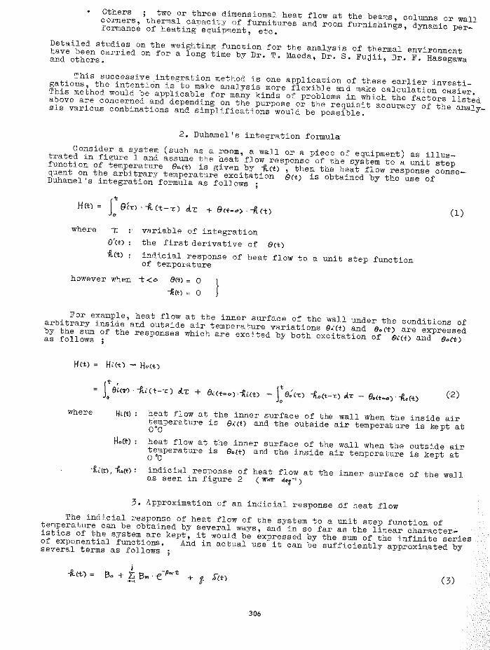
Others ; two or three dimensional heat flow at the bea~s, columns or wall corners, ther~al capacity of furnitures and room furnishings, dynamic per­formance of heating equip'Yient, etc. Detailed studies on the weighting function for the analysis of thermal enviFonment have been carried on for a long time by Dr. T .. Maeda, Dr. S. Fujii, Dr. F. Hasegawa and others ..

This successive integration method is one application of these earlier investi­gations, the intentiOn is 'to make analysis more flexible and make calculation easier. This method would be applicable for many kinds of problems in which the factors listed above are concerned and depending on the purpose or the requisit accuracy of the analy­sis various conbinations and simplifications would be possible.

2. Duhamel's integration formula-Consider a system (such as a room, a wall or a piece of equipment) as illus­trated in figure 1 and assu.-'lle the heat flow response of the system to a unit step function of temperature &(.l.<t) is given by i:..<t) , then the heat flow response conse­quent on the arbitrary temperature excitation $(t) is obtained by the use of Duhamel's integration formula as follows ;

HCtl t L Eli-r> -~c~-"l <ir + ect-~> .-Jt(~l (1)

where t:

e'«> iCtl

variable of integration the first derivative of 8(t)

indicial response of heat flow to a unit step function of temperature

however when -t <o 8(+) = 0 -Ji(t) " 0 }

For example, heat flow at the inner surface of the wall under the conditions of arbitrary inside and outside air tem-perature variations e..:Ct) and 8o(T) are expressed by the sum of the responses which are excited by both excitation of Bi(-t) and 8~:d:t) as follows

where Kc(t)

(2)

heat flow at the inner surface of the wall when the inside air t"emperature is e ... ·(t) and the outside air temperature is kept at 0°0

~ofr) heat flow at the inner surface of the wall when the outside air temperature is &olt) and the inside air temperature is kept at 0 °C

'fltt)' -J;,(t) : indicial resnonse of heat flow at the inner surface of the wall as seen in figure 2 ( W"<>.tr <t";- 1 )

3. Approximation of an indicial response _Qf heat flow The indicial response of heat flow of the system to a unit step function of temperature can be obtained by several ways, and in so far as the linear character .... istics of the system are kept, it wouJd be expressed by the sum of the infinite series of exponential functions. And in actual use it can be sufficiently approximated by several terms as follows ;

-il(-t.) " (3)

306

Bo : the term for steady state heat flow ( WP.tr. dE::J- 1 )

&"(t): delta function

} imaginary thermal canacity of the system ( w~:rt--?.· de3-')

prn fm. becomes larger in order of suffix -m.

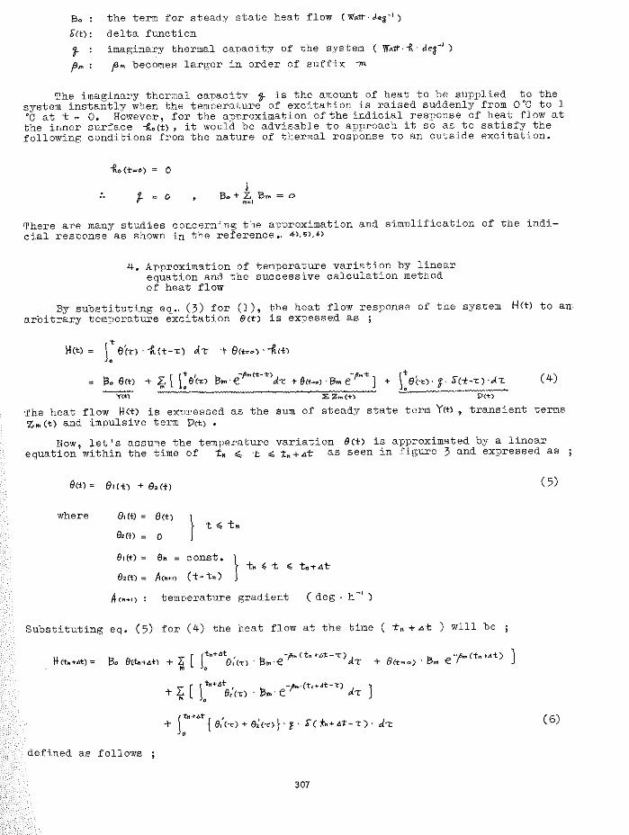
The imaginary thermal canaci ty ~ is the amount of heat to be supplied to the system instantly when the tem~erature of excitation is raised suddenly from OoC to 1 oc at t "" 0. However, for the apnroximation of the indicial response of heat flow at the inner surface -{o(t), it would be advisable to approach it so as to satisfy the following conditions from the nature of thermal response to an outside excitation.

-Ro (t:=o) 0

l .. ;.. = 0 5o+ Z. B~ = 0 m=-1

There are many studies concerning the anproximation and simplification of the indi­cial response as shown in the reference •. 4UD,6)

4. Approximation of temperature variation by linear equation and the successive calculation method o.f heat flow

By substituting eq •. (3) for (1), the heat flow resp-onse of the system HCt) to an .. arbitrary temperature excitation &tt) is expesse.d as ;

[ IT I h -p ... (1:-"1:) -p,..-t \' ao 9{t) -+ ~ oe(""t:) Drn·e d<:: +9(-t .. <>)"Bme ] + "e("1;.)·t· S(-t-<::)·J.-r:

~ :Z z.., (+) D<t)

·:rhe heat flow I.J<t) is exnressed as the sum of steady state term Yet) , transient 'Z~o~~ (t) and impulsive term P(t) •

( 4-)

terms

Now, let, s assu~~e the temnerature variation IJCt) is approximated by a linear equation within the time o.f t 11 ~ t ~ tn+.t.t as seen in .figure 3 and expressed as

( 5)

where e~ct) = e<+l } t ~ tt'l Sz(t) , 0

81(+) = e. canst. l tl'l ~ t .; t,T.At-fhCt) "" A<"+n (-t-t,)

A (" ... 1 > : temnerature gradient ( deg · h _, )

Substituting eq. (5) for (4-) the neat flow at the time ( ,t, + .ot ) will be ;

( 6)

defined as follows

307

0

e:(t) = 8z(-t) = 0. • t ~ tn

r fe-e). "ct-,:) J.-r fct) 0

-t > 0

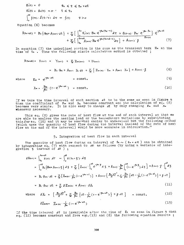
Equation (6) becomes

(7)

In equation (7) the underlined portion is the same as the transient term Zm at the time of t~~. . Thus the following simule calculation method is obtained ;

HctM+.rl)= H<n+l':l = Y(n+•) -t Ig Zmcn-t•) + D(n+l)

B,·9:n) + Ac~+') }3,·llt + ~ { Z"''"') ·"Em + Ac•a•) · Xrn}-+ Acn+•> ·; ( 8)

where Em = -e-ftot·D.t canst. (9)

canst. (10)

If we take the time interval of each section .Lit to be the same as seen in figure 4 then the coefficient of Frn and Xm. becomes constant and the calculation of eq. (8) becomes very simple. It is also easy to change At by only changing E ... and x ... whenever necessary.

This eq. (8) gives the rate of heat flow at the end of each interVal so that we are able to analyze the heating load or the temverature variations by substituting this1or eq. (16) and it may be somAwhat easier to understand but the following method (which uses the quantity of heat flow during the interval instead of thG rate of heat flow at the end of the interval) would. be more accurate in calculation.::~)

5. Integration of heat flow in each interval

The quantity of heat flow during an intervg_l of t11 ,...._,. ( t" 1- 4't ) can be obtained by integratin~ eq. (7) with resl)ect to 1:.1=" as follows (by using a variable of inte­gration ~ instead of At ) ;

-" At ,.[z 'c' "-r-··'l) +A'""'.r •:·•+'+z.. ~::{•t- i.CI-_,-r-•+>t+•·•t] v .. · t7C"l • + "i;;' tto(Kl • p... -~ l ,._ r ... r l ,-

( 11)

where JX, = [ B~At,+.(;- ;:{•t-;.(l-€-p••~)f+t·At] const. (12)

'Z z ' c -r···• tJ "'(~>= '"(") · p;, 1- e ) ( 13)

If the time interval At is invariable after the time of tn as seen in figure 4 then eq. (12) becomes constant and from eqs.(l3) and (8) the following equation results ;

308

Zlll(h-tl) ..J.. C 1- e -prn· ... t.) f·

(14)

where Ax,, ( 15)

= canst.

If the ternnerature gradients Ar"+t) , Ach .. ,.) , ······· are known, each AZ,rh+l), .6'Zm(hH)

can be easily calculated in succession by eq. (14-), and each .dHc~ .. ,1 , LlHtht-2),

is also obtained from eq. (11) by the repetition of simple calculations.

6. Equation of heat balance

(when the heat transfer coefficients of the room do not change )

Consider room k which is adjacent to ro(lms k' = 1, 2, 3, ... te"TcTJeratures are different from each other as seen in figure 5 .. equation of heat balance can be given ;

where room air The following

where

G~o:<t) , ek"(t) :

VkC+> :

(16 )

thermal capacity of t'"le air of room k ( W<~.:tt.""ft. J-es-') including that of furnishings of which the temperature change is considered the s~~e as that of the air temp.

temperature of the room and adjacent rooms

heating rate supplied to room air (W~~)

including auxiliary heat from human bodies and equipment

heatless through the surrounding walls of the room, where the air temp·. is 9k{t) and the ad;!acent room air temp. is 8k{t) = 0

inflow of the heat from the inside surface of the partitions adjacent to t1le room f< under the condition of 8k(t)= 0 ad,lacent room tlk'{t)

I< air volume infiltrated from room,..(outflow air is not related)

Cr : specific heat of the air for unit volume (1't"e:o.1t·-f\· de~- 1 · m- 3)

Assume the divisions of time are the same as in figure 4- and assume the temperature variations within the time interval t~~. .-.....(tt~+L>t) are as follows ;

8Ct.) = euo + A (h+l) • ( t- ;tl1)

(17)

And assume the heating rfl.te W<t) and the infiltration rate Tct) are constant during the time interval of ~t . Then by integrating eq. (16) with respect to t from ;t11... to ( 'th+.1t) and substituting eq. (11), the following relation is obtained ;

(continue)

309

+ ~ Laok' -eJ<(n.} -At+* L1Zml((l>) + AXok ·Aif(ll+l) + Cr·Vt<(ll+>) 'L:l't-1 61K(tt)- ek(ll) + ~t (Ak(tl-1-1) -Aieeh.J-1))}]

(18)

6.1 When the temperature is known

In eq. (18) the temperature gradients hea+;ing load Wk(n-tl) is obtained easily. By result~ the net heating load is obtained.

AkCIItl) and Ak(11Tl) are known so the total subtracting the auxiliary heat from this

6.2 \·IJhen the temperature is not known

As for unconditioned space or when intermittent heating or cooling is a factor, tbe temnerature gra/'ient A~cntl) is obtained from the following equation.

Ak (1!+1) ""

6.3 When the temperatures of adjoining rooms are not known

Nhen the building hA..s 'nany rooms or spaces of 'Vhich tearc.era --;ure variations are not given, we h':lve to solve equai;ion (19) as a shmltaneous equation of Unknown temper­ature gradients.

However, from the nature of the ther~nal rPsponse to a outside excitati··n, the influence of the temnerature variation of the adjoining room is gradual as seen in figure 2. Therefore the accuracy of the te"1perature gradient of the adjoining room Ak(~>+l) is not too important for the calculation of Ak<n·N) and this is a very fortunate charscteristic of this calculation T'l.ethod.

In this case it would be go.'>d to assume that the temperature variation of the adjoining room is the same as that at tbe time At before. That is to use Ak-<I'L) which was alreii·'y calcuJated instead of the unknown quantity Ak'<ntt) in eq_. (19).

7. When the heat transfer coefficient varies wit!'-. time or temperal;ure

Actually a fairly larp:;e vart of the heat from a hur:1an body, electricity, radiators and window sunlight, transfers by radiation to the surrounding walls and moreover the convection heat transfei· coefficient varies witb the wind velocity or with the temper­ature difference between the wall surface and the air, so that for the precise analysis of the problem it is necessary to treat the heat transfer coefficient as a val·iable.

In this case, it is alRe possi.ble to use the sarne method as above by considering each surface of the walJ , of which t':le heat transfer coeLficient is a variable, as a kind of a room where the te·nperature is not known, The order of the calculation is as follows ; -

Step 1. heat balance of the surface of the wall

An equation of heat baJance of the surface of t~1e wall at time -t and during the time interval of Lit would be written as follows ;

where

cXkA (t){ e;m- 8Wil }-Hot (t) + HkHil + ht (il = o ( 20)

l tn+..it

tn c<-~· (11-tl). { 8k{t)- Bid (t)} .J.t - 41-/k'J(JHI) T LIHk'J (n+l) + l~Hn+l) ·Lit -= 0 (21)

Jld! (11+1)

heat transfer coefficient of wall 11 J.. 11 of room k and which is constant during the time of tn...-....(tn+tt-t)

effective radiation to the surface of wall 11 J.. 11

air te~perature of room k

310

H<' Ctl

temperature of wall surface 11 .R. 11 of room -k

indicial response of heat flow of the inside surface of wall 11 fl. 11 to a unit step function of temperature of the same surface

indicial responce of heat flow of the inside surface of wall up_ n to a unit step function of temperature of the outside surface

8k~(t} : temperature of outside surface of wall 11 J. n

By substituting the following relations to the eq. (21)

e.gctl Bn.Hn.) + Ajq:J(n+l)'(t-tn)

\ 6k(11) + Ak (n+l) . (t-t.)

ek~(n) + Ald(n+l)·{t-tn)

9•Ct)

whereby

( 22)·

If the temperature gradients AR<n+l) , AJd(n+t) are not known, assuming that AR<n+l) is Ak<n) , and A~cli(l'l+l) is AkHn> , the temperautre gradient of t11.e wall surface Ald(11+1) is obtained from eq. (22).

Step 2. Equation of heat balance of the room air

After the tem-perature gradients of the surronnding wall surfaces Ak~CIHlJ are obtained the heat balance of the room air will be expreSsed as follows ;

+ 'WkCn+ll ·At

Ls sl'' {;(kA (n+l) ·At. { eh.~(n) - 81'!{11) +;; ( Ald(ntl) - AJ./:(11+11)}

'

From eq. (23) the unknown value of the temperature gradient A~tcn-t~) or the heating load 'WII.(n-+1) iS< obtained.

8. Initi~l conditions of calculation

Figure 6 shows an example of the room air temperature variation of a flat house which is built with reinforced concrete and is heated intermittently.-.. As seen in the example, if the thermal capacity of the system is large it will take many calculations

311

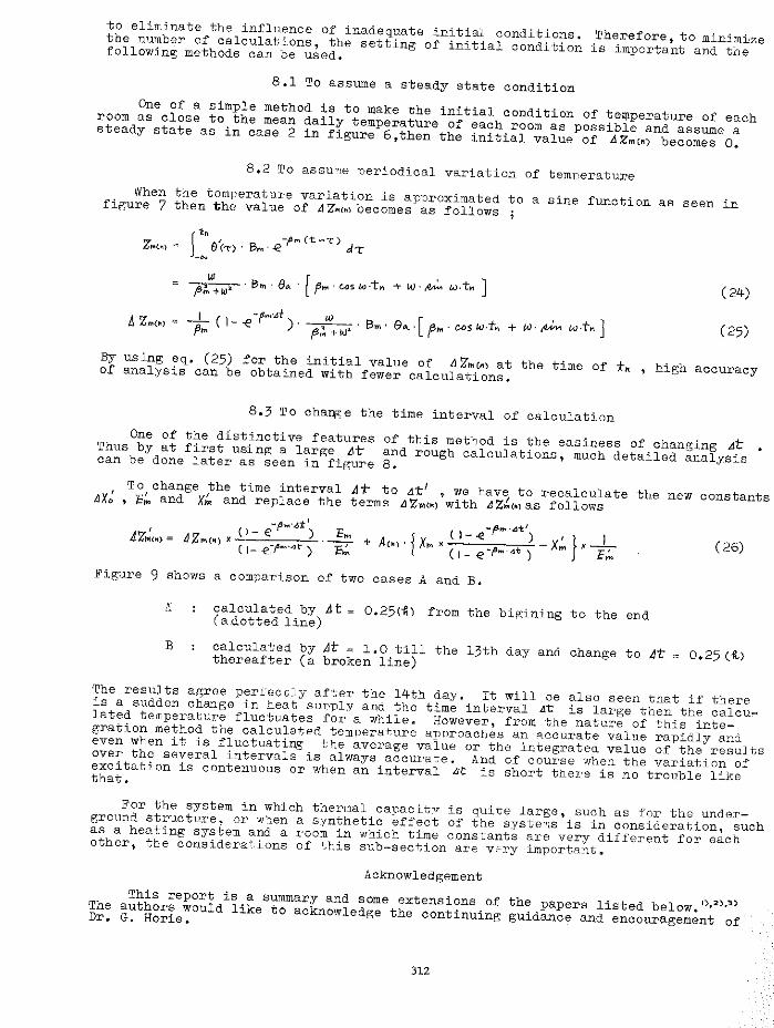
to eliminate the influence of inadequate initial conditions. Therefore, to minimize the number of calculations, the setting of initial condition is important and the following methods can be used.

8.1 To assume a steady state condition One of a simple method is to make the initial condition of te~perature of each room as close to the mean daily temperature of each room as possible and assume a steady state as in case 2 in figure 6,then the initial value of AZmcn) becomes o.

8.2 To assu~e periodical variation of temnerature When the temperature variatton is approximated to a sine function as seen in .figure 7 then the value of LI'ZI'IInl becomes as .follows ;

J1n eJ('t') > B,..,-..e-pm(t-T) dT -~

( 24-)

'" I (1 ...D-pm·Af) w Bm· e··[A~·"~'-SW·t .... + (/.)·~ w-tl1] o "•'"' " -p;;; - ' . I"~+ w• - ,-'" ~ ( 25)

By using eq. (25) for the initial value of Ll Z"t~~Cn) at the time of :tn. , high accuracy of analysis can be obtained with fewer calculations.

8.3 To change the time interval of calculation One of the distinctive features

Thus by at first using a large L\t­can be done later as seen in figure

of this method is the easiness of changing At and rough calculations, much detailed analysis 8.

To change the time interval AT to 4t1 , we have to recalculate the new constants LJX; , E~ and Xfn and replace the terms LJZt~~<n) with AZ"c~l as follows

( 26)

Figure 9 shows a comparison of two cases A and B.

,\ calculated by At"" 0.25(it) .from the bigining to the end (a dotted line)

B calculated by At " l. 0 till the 13th day and change to .dt: thereafter (a broken line) 0.25 (~)

The results agree per.i:eccly after the 14th day. It will be also seen that if there is a sudden change in heat sunply and the time interval At is large then the calcu­lated temperature fluctuates for a while. However, from the nature of this inte­gration method the calculated temPera~ure apnroaches an ~ccurate value rapidly and even when it is .fluctuating the average value or the integrated value of the results over the several intervals is always accurat:;e. And o.f course when the variation of excitation is contenuous or when an interval .1t is short thei"e is no trouble like that.

For the system in which thermal capacitv is quite large, such as for the under­ground structure, or w"_en a synthetic effect of the systw1s is in consideration, such as a heating system and a room in which time c.onstants are very different .for each other, the considera:;ions o.f this sub-section are v;:c.ry important.

The Dr.

Acknowledgement This report is a summary and some extensions of the papers listed below. l),z),;.) authors would like to acknowledge the continuing guidance and encouragement of G. Horie.

312

References

1. N. Aratani, 1 N. Sasaki and M. Enai ; Continuous calculation method for the analysis of room air temperature variations, Part 1 and Part 2, Extra Report of A.I.J, (Oct., 1968)

2. Same as above, Part 3, Extra Report of A .I .J. (Aug., 1969)

3. N. Aratani, N. Sasaki and M. Enai; A successive integration method for the analysis of room· air temperature or ther:nal load ,variations, Bulletin of Faculty of Eng., Hokkaido Univ., No. 51 (Dec., 1968)

4. T. Maeda; Some simplifications for the calculation of room air temper­ature variations, Report of A.I.J., No.27 (1954)

5·

6.

T. Maeda, M. Matsumoto and T. Naruse ; function·refered to heating in concrete (Oct., 1960)

Simplification of the weighting room, Trans. of A.I.J. No. 66

F. Hasegawa ; Three methods in room temperature analysis, Trans. of A.I.J., No. 69 (Oct., 1961)

(Papers above are writtenin Japanese)

313

exci.tation >I System

I respons}

e~(t)=l 'c h(t)

e < tl H(t)

Fig. 1 Thermal system

9~(t):$t~(t) iHt ,., ~

tns.iid.e out&iide ~((t)

e., {t) =o •• 0

9o(t)= 8u(1)

1 •c

io(t) • <- ~o(t) S~Ct) = o

0 1:

W<1t

~· H(t) ·- H<-t> 6i(t)

··~

i Fig 2, Indical response of heat flow

a /. 9<t> = e, <t) + e2 ct)

--+..------------~--~~--t 0 t. Fig. J Approximation of temperature

314

2nd day ' ~·"'~- --

fl§iit~:jjJ ••

,1t " .. AT

a I /'"

ac·tl ,/

/ t

0

Fig. 4 Division of time

I<= 3

Fig. 5 Room k and adjoining room K

3rd day 13th day ~------

\__ ( •

288

periodical heat supply

PM+! 72

periodical steady state

\..... c ~C,_,___Z __ c-'=-J.c_

••• infinite' <-« l

Fig·. 6 Intermittent heat supply and calculated room ad.r temperature::

315

a 9ct) = 9'" + e~~. sin wt

---;-_;-~ 9m

tn

Fig. 7 Assuming of periodical steady state

9 At

Fig. 8 Change of time interval

Fig. 9 Examples of calculation when /J. t is changed

316