A Systolic Algorithm for Solving Dense Linear Systems
CHAU-JY LIN Department of Applied Mathematics, National Chiao-Tung University
Hsinchu, 30050, Taiwan, R.O.C. cj lin~math, nctu. edu. tw
(Received and accepted May 1996)
A b s t r a c t - - F o r an arbitrary n x n matrix A and an n × 1 column vector b, we present a systolic algorithm to solve the dense linear equations Ax = b. An important consideration is that the pivot row can be changed during the execution of our systolic algorithm. The computational model consists of n linear systolic arrays. For 1 < i < n, the ith linear array is responsible to eliminate the ith unknown variable xi of x. This algorithm requires 4n time steps to solve the linear system. The elapsed time unit within a time step is independent of the problem size n. Since the structure of a PE is simple and the same type PE executes the identical instructions, it is very suitable for VLSI implementation. The design process and correctness proof axe considered in detail. Moreover, this algorithm can detect whether A is singular or not.
K e y w o r d s - - P a x a l l e l computer, Linear array, Systolis algorithm, Dense linear system.
1. I N T R O D U C T I O N
Paral lel compute rs have been used to solve m a n y problems in the fields of sciences and engi-
neering. Systolic array is one of parallel computers . An algor i thm which can be executed on
a systolic array is called a systol ic a lgor i thm. The systolic array has been widely used to solve
various problems because of its regular s t ructure , simple in terconnect ion, and feasibility for VLSI
i m p l e m e n t a t i o n [1-5]. Some useful discussions of systolic arrays and systolic a lgor i thms can be
referred to the papers in [6-8].
Given an a rb i t r a ry n × n mat r ix A = (ai j ) and an n × 1 co lumn vector b = (b~), the solut ion of
the l inear sys tem A x = b is one of major problems in computa t iona l and applied mathemat ics .
For solving A x = b, under the e lementa ry row opera t ion on A, a sequential a lgor i thm is always
required to find an i th pivot row such tha t this row possesses the largest absolute value among
the i th co lumn of A. This par t ia l p ivot ing me thod is not easy to be accomplished wi th in a
parallel a lgori thm. Thus , m a n y parallel a lgori thms to solve A x = b require some assumpt ions ,
such as A is nons ingula r t h a t the diagonal entr ies of A are nonzero, and tha t the problem rela t ing
to p ivot ing is not considered [9-15].
W h e n A is a nons ingula r matr ix , the L U decomposi t ion is a very useful me thod to solve
A x = b. This me thod ob ta ins a t r i angu la r ma t r ix from A followed by the back subs t i tu t ion .
T h a t is, the solut ion of A x = b comes from the solut ions of two t r i angu la r systems L y = b
This work was supported by the National Science Council, Taiwan, R.O.C., under the contract number: NSC 84-2121-M009-012.
Typeset by Jth~S-TF_ ~
77
78 c.-J. LIN
and U x = y. However, it is possible tha t there exist many nonsingular matrices in which the L U decomposition is not easy to do. For example, a zero will appear in the diagonal of A when the L U decomposition is in progress. In this article, without any assumption on the given matr ix A, we present a systolic algorithm to obtain the solution of A x = b. Under our method, an existing pivot row can be replaced by a new pivot row during the execution of the elementary row operat ion on A. If A is a singular matrix, then we can find a row or a column such tha t it
has all zero entries. The computat ional model used to solve A x = b is a two-dimensional systolic array which
consists of n linear systolic arrays. Each linear array is designed by the same consideration. Thus, these n linear arrays have similar structure and execute identical instructions. Every linear array has n equations as input da ta and also has n equations as output data. For 1 < i < n, the ith linear array is responsible to eliminate the i th unknown variable xi of x. This ith linear
array deletes (n - 1) coefficients of xi and remains the value of 1 as the coefficient of xi in the last equation. But this coefficient 1 of xi is not involved into the work of the following (n - i) linear systolic arrays which are used to eliminate the unknown variables x k for i + 1 < k < n, respectively. Hence, when we perform the instructions on the ith linear array, the unknown variables xl for 1 < l < i - 1 are all ignored. This design consideration implies tha t the back substi tut ion which is followed the L U decomposition is unnecessary in our systolic algorithm.
2. A N O V E R V I E W O F S Y S T O L I C A R R A Y
A systolic array consists of many simple structure PEs (processing elements) such tha t the same type PE executes the same instructions. Each PE only can communicate da ta with its neighboring PEs. Suppose tha t PE1 and PE2 are two PEs in a systolic array. If it is necessary to
transfer da ta from PE1 to PE2, then there exists a communication link, say ~-link, joining PE1 to PE2. The da ta sending out by PE1 on ~-link is denoted as ~out of PE1. The da ta receiving by PE2 from ~-link is denoted as ~in of PE2. This ~-link is also considered as an output link of
PE1 and an input link of PE2. In a systolic array, a t i m e s t ep is considered as an enough large elapsed t ime unit such tha t all
PEs can perform the following three tasks.
(c~) The PE reads da ta from its input links. (~) The PE executes the designed algorithm exactly once loop. (V) The PE sends out data to its output links.
In our algorithm, the elapsed t ime unit within a t ime step is independent of the problem size n. If a ~-link from PE1 to PE2 has a delay symbol ~D, then the ~out sending out by PE1 at a
t ime step t will be the ~in of PE2 at the t ime step t + $. In our systolic array, each link has only one delay, tha t is, ~ -- 1. Thus, we omit the delay symbol in our systolic array. The condition of
~ 0 means that the behavior of da ta broadcasting is not allowed within our systolic array.
3 . T H E D E S I G N C O N S I D E R A T I O N
O F A L I N E A R S Y S T O L I C A R R A Y
For a fixed integer i such tha t 1 <: i <: n, we design the ith linear systolic array to eliminate t h e ith unknown variable xi of x. The ith linear array consists of (n - i + 2) PEs and three communicat ion links with names a-link, d-link, and c-link. See Figure 1. These PEs are indexed as P E ( i , j ) for i < j _< n + 1. The d-link and c-link are used to send da ta from P E ( i , j ) to P E ( i , j + 1). The input a-link of P E ( i , j ) is used to receive da ta from the (i - 1) th linear array. The output a-link of P E ( i , j ) is used to send data to the (i ÷ 1) th linear array.
We classify our PEs into two types. The PE(i, i) is in the type I and the remaining PEs are in the type II. The structures of PEs are depicted in Figure 2. Each PE contains a register R. The type I PE has a more register P. The PE(i, i) is responsible to find a pivot row. When a pivot row had found, the type II PEs update the entries of another rows.
From the above discussion, we obtan n linear systolic arrays. These n linear arrays are con- nected to form a two-dimensional array as shown in Figure 3, where the k th column of A will be arranged to meet PE(1, k) for 1 < k < n and the column b will be arranged to meet PE(1, n ÷ 1). We use the symbols " * " and ..... to mean a waiting and a stopping signal, respectively.
Let [A (°) , b (°)] be the n × ( n ÷ 1) augmented matr ix by adjoining b to A. At the beginning of our algorithm, the matr ix [A (°), b (°)] is the input values of the a-links on the first linear array. The output data, except the symbol " *," which comes from the a-links of the i th linear array will be formed and denoted as the matr ix [A (0, b(0]. According to the order of the values appearing on the output a-links of the i th linear array, the row indexes in [A (i) , b (0] are numbered sequentially as i + 1, i ÷ 2 . . . . . n, 1 , 2 , . . . , / . T h a t is, the first aout of P E ( i , j ) has the row index (i + 1) in
80 C.-J. LIN
[A(i),b (~)] and the last aout of PE( i , j ) has the row index i in [A(i),b(0]. Of couse, this matr ix [A (i), b (i)] will be the input data of the (i + 1) th linear array.
Note that the matrix [A (i), b (i)] is an n × (n - i -}- 1) matrix since PE(i, i) has no output a-link. The absence of output a-link in PE(i, i) causes the ith unknown variable xi to be deleted. The solution of A x = b will appear on the aout of PE(n, n + 1) which is on the n th linear array.
In our systolic array, the d-link is only used to carry the ain of PE(i, i) to PE(i, j ) , for all j > i. The major work of the c-link is to indicate whether a new pivot row is found or not. At the initial state, we assign ( n - i + 1) to the register P of PE(i, i). When the first pivot row is found, we reset P as 1 - P. This value of 1 - P indicates how many remaining rows will be tested as a pivot row. The register R of PE(i, j ) contains an entry of the current pivot row. At the initial state, we set the symbol " * " into the register R of all PE( i , j ) .
4 . T H E I N S T R U C T I O N S O F P E S
For 1 < i < n and i < j _< n + 1, we will present the major instructions of PE( i , j ) . All PEs perform their instructions until the signal . . . . . appears on their input a-links. First, we consider
the work of type I PE.
(1) The main purpose of PE(i, i) is to find the first pivot row by detecting its first nonzero value of ain. Once PE(i, i) has found its first pivot row, PE(i, i) performs the following three tasks. ((~) PE( i , i ) sets its P = 1 - P. (~) PE( i , i ) assigns lain], the absolute value of ain, into its R.
(V) PE( i , i ) sends ain to its d-link. (2) If PE(i , i) has its P > 0 and ain ---- 0, then PE( i , i ) is still on the state of finding the first
pivot row. Tha t is, the first pivot row is not appeared until now. In this case, PE(i, i) decreases one from P and PE(i, i) continues its search of the first pivot row. At any time step, once PE( i , i ) has its ain ~ 0, PE( i , i ) sets its Cout ---- 1 in order to detect whether there exists a zero row in the matrix A (i-1). The existence of a zero row in A (i-l) causes
the singularity of A. (3) If there exists no pivot row, we obtain P = 0 and R -- * in PE(i, i). Tha t is, the first
column of A (i-1) will be appeared as a zero column. In this case, PE(i, i) announces that A is a singular matrix by sending the message of its Cout = 3.
(4) After PE(i, i) had found a pivot row and PE(i , i) has its P < 0, if PE(i , i) has ain ~ 0 again, then PE(i, i) tries to replace the existing pivot row. When lainl > R, the action of exchanging two pivot rows will be performed. This exchanged message is transferred by a value of 2 on the c-link.
Now we consider the major work of the type II PE. These PEs will be used to modify the entries of [A (i-1), b (~-1)] into the entries of the matrix [A (i), b(i)].
(5) P E ( i , j ) always sends its din to dour. (6) If PE(i , j ) knows that PE(i , i) had found its first pivot row, then PE(i, j ) assigns the value
of a in /d in to its R. At this same time step, PE(i, j ) sends out the symbol " * " to its aout. (7) If PE(i , j ) has its Cin = 0 and R ¢ *, then PE(i, j ) modifies the value of its ain into the
value of its aout.
(8) When P E ( i , j ) has its cin = 1, P E ( i , j ) detects whether its ain = 0. If ain -~ 0, then P E ( i , j ) passes its cin to Cout- Otherwise, if ain ¢ 0, P E( i , j ) sets its Cout = 0. This work detects whether there exists a zero row in A (i-1). When PE(i, n) has its Cout = 1, we know that A is a singular matrix because of a zero row in the matrix A (i-1).
(9) If P E ( i , j ) has its Cin -- 2, then the action of exchanging two pivot rows is performed. The PE(i , j ) retrieves the content of R to be modified into its aout and PE(i , j ) stores the new pivot entry a in /d in into its register R.
(10) When P E ( i , j ) has ain = , PE( i , j ) sends the content of its R to its aout and P E ( i , j )
Systolic Algorithm 81
resets R as a special symbol "&" in order to send the signal " ^ " to its aout a t the next
t ime step.
5. T H E S Y S T O L I C A L G O R I T H M
Firs t of all, we define n ine procedures. The first five procedures are used in the type I PE. The
last four procedures are used for the type II PE.
p r o c e d u r e t e s t i ng - f i r s t -p i vo t
i f P - - 1 t h e n s e n d i n g - s i n g u l a r - m a t r i x e l se searching- f i rs t -p ivot .
p r o c e d u r e s e n d i n g - s i n g u l a r - m a t r i x - Cout -- 3; R = ^ .
p r o c e d u r e search ing- f i r s t -p ivo t =_ P = P - 1; Cout -- 1.
p r o c e d u r e f i nd ing - f i r s t -p i vo t -- P = 1 - P ; R = laini; Cout = 0.
p r o c e d u r e t r y i n g - n e w - p i v o t =-
P = P + I ;
i f lainl > R t h e n ( R = lainl; Cout -- 2} e l se ( i f a i n = 0 t h e n Cout = 1 e l se Cout = 0.}
p r o c e d u r e s e n d i n g - l a s t - e l e m e n t -- aout ~- R; R --- ~ .
p r o c e d u r e exchang ing - two-p i vo t s - aout = R - a i n / d i n ; R : a i n / d i n .
p r o c e d u r e modi f y ing -a - l i nk -
i f R -- • t h e n s tor ing - f i r s t -p i vo t e lse aout = ain - R * din.
p r o c e d u r e s tor ing - f i r s t -p i vo t - i f din ~ 0 t h e n ( R -- ain/din; aout -- *} e l se aout -- ale.
ALGORITHM. L I N E A R - S O L V E R (A, b, n) -
I n i t i a l s t a t e :
For l < i < n a n d i < j < _ (n + l ) , we set R = . in all PEs. S e t P = n - i + l i n P E ( i , i ) . The
en t ry ai,3 of A meets PE(1, j ) at the t ime step t -- j + i - 1. The en t ry bi of b meets PE(1, n + 1)
at the t ime step t -- n ÷ i. A s topping signal " ^ " will meet P E ( 1 , j ) at the t ime step t -- n + j .
All the r ema in ing links are denoted by the symbol "* "
E x e c u t i v e s t a t e :
r e p e a t
/* d o p a r a l l e l fo r a l l P E s o f t y p e I . * /
dnut ~ ain; if ain ~- * t h e n (Cout = *; b r e a k } ;
i f a i n - - ^ t h e n ( R -- ^ ; Cou t ---- ^ ; b r e a k };
if P = 0 t h e n Cout = 0;
if P < 0 t h e n t r y ing -new-p ivo t ;
if P > 0 t h e n { if a i n ---- 0 t h e n t e s t ing- f i r s t -p ivo t e l se f ind ing- f i r s t -p ivo t} ;
/ , d o p a r a l l e l fo r a l l P E s of t y p e I I . */
dout -- din;
i f ( C i n ~ - 1 a n d ain ~ 0) t h e n Cout = 0 e l se Cout = t i n ;
i f ain : * t h e n (aout --- *; b r e a k ; }
i f (R = & o r ci, = 3) t h e n ( R = ^ ; a o u t ---- ^ ; b r e a k ; }
i f a i n : ^ t h e n ( send ing - la s t - e l emen t ; b r e a k ; }
if Cin = 2 t h e n exchang ing- two-p ivo t s ;
i f (Cin = 0 o r Cin = 1) t h e n modi fy ing-a- l ink ;
u n t i l R = ^.
6. A N I L L U S T R A T I V E E X A M P L E
We give an example wi th
0
- 7 - 4 2
82 c.-J. LIN
to i l l u s t r a t e our a lgo r i t hm as shown in Table 1. The re la ted values of Table 1 are co r re spond ing
to t he pos i t ions of l inks and regis ters as shown in F igures 1 and 2, where the ar rows are omi t t ed .
In w h a t follows, we use the n o t a t i o n " P E ( i , j ) [ a ; , = 2, R -- 3 , . . . It = 4" to ind ica te t h a t P E ( i , j )
has i ts ain -- 2, R -- 3, and so on a t t he t ime s tep t = 4. T h e symbol "S1 ==~ $2" means t h a t the s t a t e m e n t S1 impl ies the s t a t e m e n t $2.
Table 1. An illustrative for n = 3 (the first linear array).
Time PE(1,1) PE(1,2) PE(1,3) PE(1,4)
* = t { - { { - { { - { 0 ~' ,t * •
t • t ~ *
2 * * t
• t
4 - 1 * t
t t
3 1 1 *
~ C i:)0 ~ ~ V ~ ~ V ~ : V ~ : -3/4
^ -7 0 5
4 ~ ^ ^ ~1-~-I ~o 4[ o-1'2 o~1-~. ~o -31/4 1/2
^ -4 3 ^ A 3 4
5 ~ A [ & ' ~ ^ 3 I ~ O 1 0 2 F ~ ' - - - I 4 2 "114 -4 7/4
^ 2
° I-:--I ^^I-71 ^̂ o~ I-~13o ^ 0 -1/4
A
V:~ [ ~ ^^~1 ^̂ ^ 3/4
A
T h e r e are t h ree l inear equa t ions which co r respond to the l inear sys t em A x = b.
2Xl - x2 + x3 -- 5, (1)
4x l + z2 = 3, (2)
3 x l - 7x2 - 4x3 = 2. (3)
In Table 1, th ree l inear sys tol ic a r r ays are considered in the following th ree cases, respect ively.
CASE ( a ) . On the first l inear array, since PE(1 ,1) [a in = 2, P = 3]t = 1, t he equa t ion (1) is a
p ivot row. F r o m the p rocedures f i n d i n g - f i r s t - p i v o t and s t o r i n g - f i r s t - p i v o t , we have
PE(1 , 1) [P = - 2 , R = 2, dout = 2, tout = 0] t = 1,
Systolic Algorithm
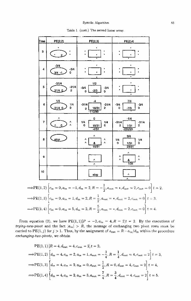
Table 1. (cont.) The second linear array.
83
rime PE(2,2} PE(2,3)
. :-1
10
.3/4 • < E b -3" " . - 7
0 * *
.31/4 1/2 0 3114 -3/4 ~ - 3 / 4 2 0 0
1/4 -4 ~ 1/4 .31/4r~-~ .3114
0 2 l ,olo, i 2 .110/93
^ 0 ( ~ ) ^̂ 1/4 ~ 1 1 4 0 0
-4/31
^ E l ^ A ^
16/31
A
PE(2,4}
. .-i- t
• .7. =
: I - ]
7/4 -3/40 ~ ' ~ 0"3/4
-1/4 - 3 1 / 4 [ ~ 2"31/4
-220193
3/4 1140 [ ~ 01/4
23/31 A
^ ~ - ~ ^ A A
1/31
A
===~PE(1,2) Icin =O, ain = - l , d i n = 2, R = - 2 , a o u t =* ,dou t = 2, Cout =O] t = 2,
==~PE(1,3) [Cin = O, ain = l ,din = 2, R = ~,aout = . ,dout = 2, Cout = Ol t = 3~
===aPE(I,4) [Cin = O, ain = 5, din = 2, R = 5,aout = *,dout = N, cout = Ol t = 4.
From equa t ion (2), we have P E ( 1 , 1 ) [ P = - 2 , ain = 4, R = 2It - 2. By the execut ions of
trying-new-pivot and the fact lain[ ::> R, the message of exchanging two p ivot rows mus t be
ca r r i ed to PE(1 , j ) for j > 1. Thus , by the ass ignment of aou t = R -a in /d in wi th in the p rocedure
exchanging-two-pivots, we o b t a i n
PE(1 , 1 ) [R = 4, dout = 4, Cout = 2] t : 2,
- - - ~ P E ( 1 , 2 ) din = 4, Cin = 2, ain = 1,aout = - ~ , R = ~,dout = 4, Cout = 2 t = 3,
----~PE(1,3) [din = 4, cin = 2, ain -= O, aout = l , R = O, dout = 4, Cout = 2] t = 4,
==aPE(I ,4) [din = 4, Cin = 2, ain = 3, aout = 7 , R = 3,dout = 4, Cout = 2] t = 5.
84 C.-J. LIN
Table 1. (cont.) The third linear array.
Time
5
PE(3,3) PE(3,4)
!
7 -110/93
-110/93 0
1 I ,t
1 I * . t
10
11
-4/31 -4/31 0
16/31 16/31 0
A
A
-220/93 "110/93 I 0 2 I "110/93 0
23/31 -4/310 ~ - ~ 0-4/31
1
1/31 16/31 16/31 o lo
:1 A
I - 1 A A
2
12 F 1 A
T h e a b o v e t h r e e va lues of aou t f o rm t h e f irst row of [A(1),b (1)] w i t h row i n d e x 2. F o r equa -
t i o n (3), b y t h e p r o c e d u r e trying-new-pivot w i t h ]ainl -- 3 < R a n d the e x e c u t i o n of t h e a s s i g n m e n t
aout - - a i . - R * din w i t h i n t h e p r o c e d u r e modifying-a-link, we have
P E ( 1 , 1) [P -- - 1 , ain = 3, R = 4, dou t - - 3, Cout = 0] t - - 3,
- - - - *PE(1 , 2 ) ain = - 7 , din = 3, cin = O,R = 1 , a o u t = - - ~ - , out 3, eout = 0 t = 4,
= ~ P E ( 1 , 3) [ain -- -4 , din = 3, tin --- 0, R -= 0, aout --=- - 4 , dout = 3, tout - - 0] t = 5,
[ 3 1 ] = = ~ P E ( 1 , 4 ) ai~ = 2, din = 3, ei~ = O,R = ~ , a o u t = - ~ , d o u t = 3,¢out = 0 t = 6.
T h e a b o v e t h r e e va lues of aout f o rm t h e s e c o n d row of [A (1), b (1)] w i t h row i n d e x 3. F r o m t h e
i n i t i a l s t a t e of ou r a l g o r i t h m , we have PE(1, j )[ain = ^ ]t = j + 3 for 1 _< j < 4. Hence , P E ( 1 , 1)
s t o p s i t s e x e c u t i o n a t t = 4. F r o m t h e p r o c e d u r e sending-last-element, we have
P E ( 1 , 2) ain -~ , aout -~ "~, R = & t = 5, P E ( 1 , 3) [ain -- , aout - - 0, R = &] t = 6,
a n d 3 P E ( 1 , 4 ) a i , = ' a ° u t -- 4 '
Systolic Algorithm 85
__3 4
[A(1) b(1)] = 31 ' 4
1
which corresponds to the linear sys tem of
The above three values of aout form the third row of [A (1), b (1)] with 1 as its row index. Then we have PE(1 , j ) [aou t = , R = ^ I t = j + 4 for 2 <_ j <_ 4. Thus, these three PEs stop their executions.
From the above executions, we obta in
1 7
1 - 4 - ~ ,
3 0 3
7
- x 2 - 4 x 3 = - ~ , ( 5 )
x l + x2 = - . (6) 4
CASE (~). On the second linear systolic array, [A (1), b (1)] is the input da ta on the input a-links of P E ( 2 , j ) for 2 _< j <_ 4. From equat ion (4) and eE(1,2)[aout = - 3 / 4 ] t = 3, we have
PE(2 ,2 ) ain - 4 ' 4 '
[ 3 1 2 3 ] ===~PE(2, 3) Cin = 0, din -~ - ~ , ain ----- 2 ' R = - ~ , aout ~- *, dout -- - 3 ' Cout -- 0 t = 5,
[ ] ---~ P E ( 3 , 4 ) c i . = 0, din = -3,ai. = 3 , R = - g , a o u t = * ,dout = - - ~ , C o u t = 0 t = 6.
From equat ion (5) and the procedure exchanging-two-pivots with lainl > R, we have
[ ] 31,R = ,dout = --~-,Cout = 2, P = 0 t = 5, PE(2 ,2 ) ain - 4
31 II0 16 31 ] = 2, din ---- - -~ - , a in -- - 4 , aout - , R -- ~- ,dout -- - - T , Cout --- 2 t -- 6,
- -2 , din = - ~ - , a i n = - ~ , a o u t - - , R = ~-~, out = - Cout = 2 t = 7.
values of aou t form the first row of [A (2), b (2)] with row index 3. From equa-
~ P E ( 2 , 3) [CAn
:===~PE(2, 4) [Cin
The above two t ion (6), we have
BE(2, 2)
==~PE(2, 3)
==*-PE(3, 4)
1 31 1 ] ain ---- 4 ' R - - - 4 ' d°ut : 4 ' C ° u t - - 0 t - - 6 ,
[ 16 4 d 1 1 CAn : O, din ---- 1 , ain ---- 0, R : ~ , aout ---- - ~ - , out : 4 ' C°u t : 0 t : 7,
CAn = 0, din ---- 1 , ain = 4 ' ~ - , aout ---- ~ - , out : 4 ' tout : 0 t : 8.
The above two values of aout form the second row o f [A(2),b (2)] with row index 1. Now PE(1,2)[aout -- ^ ]t -- 6 implies PE(2, 2)[al, -- ^ ]t = 7. In the same way, we have
B E ( l , 3 ) [ a o u t = ^ ] t = 7 and BE( l , 4 ) [ a o u t = ^ ] t = 8 ,
[ ] [ ] ~ P E ( 2 , 3 ) aln = ^ , a o u t - - - ~ , R - - ~ : t = 8 and PE(2 ,4 ) ain ---^ , a o u t = l , R = • t = 9.
86 C.-J. LIN
These two values of aout form the th i rd row of [A (2), b (2)] wi th row index 2. s tep, PE(2, j ) s tops its execution.
Until now, we have the ma t r i x 110
31 1_6 31
which cor responds to the linear sys tem of
220
23
31 '
1
3 1
After this t ime
- x 3 - - 9 3 ' ( 7 )
x l - z3 = ~ , (8)
1 z~ + z 3 = - - . (9)
31
CASE ( ~ ) . We consider the opera t ions on the th i rd linear array. Equa t ion (7) is a p ivot row.
Hence, it implies
[ 110 110 . 110 ] BE(3 ,3 ) a i n - - - - - ~ - , R - - - ~ , d o u t - - - - - ~ , C o u t = 0 , P = 0 t = 7 ,
[ 110 _1 0 ] ==~PE(3, 4) Cin = 0 , din - 93 ' ain -- - , R = 2, aout = *dout = 93 ' Cout = 0 t = 8.
F rom equat ion (8), we have
P E ( 3 , 3) a i . = - ~ - , dout = - 3 i - ' P = 0, Cout = 0 t = 8,
~ P E ( 3 , 4 ) Cin = 0 , d in = -~,R = 2, a~ , = ~- i - , aou t = 1 , d o u r = - g i - , e o u t = 0 t = 9.
This o u t p u t of aout = 1 forms the first row of [A (3), b (3)] wi th row index 1. Note t h a t in this last l inear array, the ma t r i x A (a) is empty. F rom equat ion (9), we have
[ 16 ~ 16 p = O , c o u t = O l t = 9 ' PE(3 , 3) ain = ~ ' , R = ' d°ut = 31 '
[ 10 ] ~ P E ( 3 , 4 ) Cin = 0, di, = -~,ai , = ,R = 2, aout = -1 ,dou t = ~-~,Cout = 0 t = 10.
This aout = - 1 is the only en t ry in the second row of [A(a),b (3)] with row index 2. Since P E ( 2 , 3 ) h a s i t s a o u t = ^ a t t = 9, w e h a v e P E ( a , a ) [ a i n = ~ ,R = ^ ] t = 10. A t t h i s s a m e t i m e
step, PE(3 , 3) s tops its execution. Also we have PE(2, 4)[aout = ^ ]t = 10 which implies the result
of PE(3 ,4) [a in -- ^ ,aout - - 2, R -- &]t = 11. Th i s aout -- 2 is in the th i rd row of [A (3), b (3)] wi th row index 3. Finally, we have PE(3 , 4) has
its R = ^ , aout ---- ^ at t ---- 12, and thus, all PEs s top their executions. T h e solut ion of Ax = b is in the m a t r i x [A (3), b (3)] which corresponds to the linear equat ions of Xl -- 1, x2 -- - 1 , and
X3~2.
7. T H E C O R R E C T N E S S P R O O F
From the procedure sending-first-pivot, we know t h a t when the first pivot row is found by PE( i , i), the t ype I I P E ( i , j ) sends out a symbol " * " to its aout. These symbols " * " which are genera ted by the i t h l inear a r r ay will p ropaga t e to the P E s of the following k t h l inear a r ray for k > i. These synbols " * " and the wai t ing symbol " * " given in the initial s t a te of our a lgor i thm will cause some P E s to be idle.
Systolic Algor i thm 87
LEMMA 1. On the i TM l inear array, when we ignore the " * " due to the ini t iM s ta te , but we
include the " * " g e n e r a t e d by the prev ious l inear array, the first e n t r y on the i npu t a -Bnk o f
PE( i , j ) a p p e a r s a t the t ime s t ep t = i + j - 1.
PaOOF. F r o m the in i t ia l s ta te , for 1 _< j _< n, we ob t a in P E ( 1 , j ) [ a i n = ul,Jl c-(°)~ ̀ = j . Also we have
P E ( 1 , n + 1)fain = b~°)]t = n + 1. Since there is one t ime de lay on each a- l ink, by induc t ion
on the integer i, P E ( i , j ) has an en t ry on its a- l ink a t the t ime s tep t = j + i - 1 for i <_ j _<
n + l . l
LEMMA 2. On the i TM l inear array, i f we have the e n t r y a(ki~ 1) = 0, for a11 i < k < n, then PE( i , i)
send ou t i t s Cout = 3 before the t ime s t ep t = n + 2i - 2.
PROOF. By the p rocedure test ing-f irst-pivot , we know t h a t the case of all _(i-1) ak,i = 0 will be
d e t e c t e d by P E ( i , i ) on the i th l inear array. F rom L e m m a 1, P E ( i , i ) has i ts first e n t r y on its A i - i )
i n p u t a - l ink at t = 2i - 1. Since ui, i is t he first en t ry of the first co lumn of A (~-i) and the re
are a t mos t (i - 1) symbols " * " gene ra t ed from the previous (i - 1) l inear ar rays , P E ( i , i) has _ ( i - 1 )
the e n t r y (ti# on its inpu t a - l ink before the t ime s tep t = 2i - 1 + (i - 1) = 3i - 2. Thus , h(i-1) P E ( i , i) has i ts ain ---- an, i before t = (3i - 2) + (n - i) = n + 2i - 2. At th is t ime s tep, P E ( i , i)
has P = 1 and ai~ = 0. T h e p rocedure sending-s ingular-matr ix impl ies t h a t P E ( i , i) sends its
corn = 3 to ind ica te the s ingu la r i ty of A. |
LEMMA 3. During the execut ion on the i th l inear array, i f there ex is ts an integer k, for i < k < n ~(~-i)
such tha t the entries ~k,j = O, for all i <_ j <_ n, then PE( i , n) has i ts Cout = 1 before the t ime
s t ep t = n + k + i - 2.
PROOF. By L e m m a 1, the first e n t r y ain of P E ( i , i) a ppe a r s a t t = 2 i - 1. Since the first ( k - i + 1)
rows of [A ( i-1) , b (i-1)] are indexed sequent ia l ly from i to k, and there are a t mos t ( i - 1) symbols
" * " gene ra t ed by the previous (i - 1) l inear ar rays , the e n t r y a2i~ -1) will mee t P E ( i , i) before the ~(~-i)
t ime s tep t = 2i - 1 + (k - i) + (i - 1) = 2i + k - 2. By uk# = 0, P E ( i , i) has i ts Cout = 1 by the
execu t ion of p rocedure searching-first-pivot or the p rocedure t ry ing-new-pivot . Thus, we have
PE(i, i) fain = 0, Cou t = 1] t ~ 2 i + k - 2,
[ (~-~) ] = = * P E ( i , i + 1) Cin = 1,ain = 0 = ak,i+l,Cou t = 1 t <_ 2i + k - 1,
~ P E ( i , n ) [Cin = 1, a in = 0 , Cout =1 ] t < 2 i + k - 2 + ( n - i ) = n + k + i - 2.
T h e Cout = 1 on P E ( i , n ) ind ica tes t h a t A (i-1) has a zero row. Therefore , A is a s ingular
ma t r ix . F r o m L e m m a s 2 and 3, we know t h a t if the re exis ts an integer i such t h a t P E ( i , n) has
i ts Co,t = 1 or Cout = 3, t hen A is s ingular . In the following th ree lemmas , we assume t h a t A is
nons ingular .
LEMMA 4. The t ype I PE( i , i) s tops i ts execut ion at the t ime s t ep t = n + 3i - 2 and the
t ype H P E ( i , j ) s tops i ts execut ion at the t ime s tep t = n + 2 i + ] - 1. Tha t is, we have
PE( i , i ) [R = ° It = n + 3i - 2 and P E ( i , j ) [ R = ^ , aout = ~ }t = n + 2i + j - 1, for 1 < i < n and
i < j < n + l .
PROOF. By induc t ion on i.
Basis: For z = 1. F rom the ini t ia l s ta te , we have
a(°) ] P E ( 1 , 1 ) a i , = 1 , 1 ] t = 1 ,
a(0) ] ==*PE(1, 1) a in =- 1,n] t ---- n ,
==*PE(1 ,1 ) fain = ' , R = ^ ] t = n + 1.
88 C . - J . LIN
From the initial s ta te , we know tha t the en t ry of the first row of [A (°), b (°)] meets P E ( 1 , j ) a t the t ime s tep t - - j + i - 1. Since each column in [A(°),b (°)] has n entries, we have
= n + j - 1, a ( ° ) . ] P E ( 1 , j ) ain = n,3] t
= ~ P E ( 1 , j ) [ai, = ^ , R = & I t - - n + j ,
= = ~ P E ( 1 , j ) [ R = ^ , a o u t = ^It = n + j + 1.
Thus , it is t rue for i -- 1.
A s s u m p t i o n : For i -- k, it is t rue. Thus , we have
B E ( k , k ) [R = ^ I t = n + 3 k - 2,
and
P E ( k , j ) [R : ^ , a o u t : ^ I t : n + 2 k ÷ j - 1,
I n d u c t i o n : For i = k + 1.
F rom the above a s sumpt ion wi th j = k + 1, we have
f o r j > k ÷ l .
PE(k , k + 1) [aout = ^ ] t = n ÷ 2k + (k ÷ 1) - 1 = n ÷ 3k,
===~PE(k + 1, k ÷ 1) [ a i n - - ^] t ---- n ÷ 3k + 1 = n + 3(k + 1) - 2,
==~PE(k + 1, k + 1) [R = ^ I t = n + 3(k + 1) - 2.
F rom the above a s sumpt ion wi th j > k + 1, we have
P E ( k , j ) [R = ^ I t -- n + 2k + j - 1,
==~PE(k, j ) [aout ----^ ] t ---- n + 2k + j - 1,
.~PE(k + 1, j ) lain = ^ , R = &] t = n + 2k + j ,
Thus , i = k + 1 is t rue. Therefore , the l e m m a is proved by induction. |
LEMMA 5. The t i m e c o m p l e x i t y o f our s y s t o l i c a l g o r i t h m is 4 n .
PROOF. Let i = n and j = n + l , in L e m m a 4. We have PE(n , n + l ) [ R = ^ ]t = n + 2 i + j - 1 = 4n .
Thus , P E ( n , n + 1) s tops its execut ion a t the t ime s tep t = 4n. |
LEMMA 6. The i t h / /near a r r a y p r o d u c e s the values O#aout t o form the m a t r i x [A (i), b (i)] w h i c h
c o r r e s p o n d s t o t h e / / n e a r sys t em o[
(~) . a ( i ) ~ (i) h(i) a i + l , i + l X i + l T i + 1 , i + 2 ~ i + 2 ÷ • . • ÷ a z + l , n X n = V i + l ,
(i) - a (i) a (i) x = b (~) a i + 2 , ~ + l X i + l ' ~ i + 2 , i - ~ 2 X i + 2 ÷ "" " ÷ i + 2 , n n i~-2 ,
a(i) x -F ^(i) x + + a (i) x b (i) n , i + l i + 1 t~n,iq- 2 i-t-2 " ' " n , n n = n ,
- - a (i) x + ~(i) x + + (i) b~i), X l --r 1 , i + 1 i + 1 t ~ l , i + 2 i + 2 " "" a l , n X n =
(i) _ h!~) _ (i) a (i) X" ÷ + a i , n X n - z " X i t a i , i + l X i + l -{- i , i + 2 z + 2 " " "
PROOF. B y the m a t h e m a t i c a l induct ion on i.
Systolic Algorithm 89
B a s i s : For i -- 1. From the initial state, the matr ix [A, b] = [A (°), b (°)] is assigned to the input a-links of P E ( 1 , j ) ,
1 < j < (n + 1). Thus, we have PE(1, 1)[ain "(°)1÷ k for 1 < k < n.. _ _ ~ ~ k , l J ~ ~---
Suppose tha t _(0) is the first nonzero value meet ing PE(1, 1) at the t ime step t = u. Since ~u,1 PE(1 , 1)[P = n]t = 1, the procedure testing-first-pivot causes the searching-first-pivot to be executed for ( u - 1) times. Thus, we have P E ( 1 , 1 ) [ P = n - u + 1]t = u - 1. At the next
t ime step, we have PE(1, 1)[ain ¢ 0]t = u. From the execution of finding-first-pivot, we have B E ( 1 , 1 ) [ P = - n + u]t = u.
From the t ime step t = 1 to the t ime step t = u - 1, PE(1, 1) sets its Cout = 1 and dour = 0.
This causes the type II PE(1, j ) assigning its ain to its aout by the assignment of aout = ain within
the procedure storing-first-pivot under the condit ion of din = 0. T h a t is, for 2 <_ j < (n + 1), P E ( 1 , j ) carries the first (u - 1) rows of [A (°), b(°)], under deleting the first column of A (°), to form the first (u - 1) rows of [A(1),b(1)]. These (u - 1) rows in [A(1),b (1)] are numbered as the
row indexes from 2 to u.
Since the u TM row of [A (°), b (°)] is the first pivot row found by PE(1, 1), we obta in din ¢ 0 on
P E ( 1 , j ) for 2 < j _< (n + 1). From the procedure storing-first-pivot, we have
[a o ] P E ( 1 , j ) R = ~ i n , a O u t = * t = u + j - 1 , for 2 _< j <_ (n + l).
From the t ime step t = u + 1 to t = n, PE(1, 1) sends the message to indicate whether the
act ion of exchanging pivot row occurs or not. This implies t ha t the type II PE(1, j ) modifies the last ( n - u ) rows of [A (°), b (°)] to form the rows of [A (1), b (1)] with the row indexes from u + 1 to n.
Until now, we obta in (n - 1) rows in [A 0), b(1)]. These (n - 1) rows of [A (1), b (1)] correspond to
(n - 1) linear equat ions such tha t all the coefficients of Xl are deleted.
At the t ime step t = n + 1, PE(1,1) receives the s tooping signal ain = ^ • So PE(1,1) stops its
execution. Similarly, we have PE(1, j ) [a in = ^ It = n + j , for 2 _< j < (n + 1). The procedure
sending-last-element causes P E ( 1 , j ) to assign the content of R to aout to form the last row of
[A (1), b(1)]. This last row has its index 1 and it corresponds to a linear equat ion such tha t its
coefficient of the unknown xl is 1. Therefore, the case of i = 1 is true.
A s s u m p t i o n : Suppose tha t this l emma is t rue for i = k.
I n d u c t i o n : For i = k + 1. Since the values on the ou tpu t a-links of the k TM linear ar ray form the matr ix [A (k), b(k)], this
mat r ix is the input of a-links of the (k + 1) th linear array. By L e m m a 1, we know tha t the first
en t ry genera ted by the k TM linear array meets P E ( k + 1, k + 1) at t = 2k + 1.
For k + 1 < r < n, let ~(k) meet P E ( k + 1, k + 1) at the t ime step t = t~. Since there are k ~r,k-I-1 symbols " * " generated by the previous k linear arrays, the tr has to satisfy the condit ion of
2k + 1 < tr < n + 2k. Suppose tha t .(k) is the first nonzero value meet ing P E ( k + 1, k + 1) at - - - - ~ v , k + l
(k) the t ime step t = tv, for k + l < v < n. T h a t is, we have as,k+ 1 = 0, for s satisfing k + l < s < v - 1 . Hence, from the t ime step t = t~ + j - k - 1 to t = t~ + j + v - 2 k - 2, the type II P E ( k + 1 , j ) carries the first (v - k - 1) rows of [A (k), b(k)], under deleting the first column in A (k), to form
the first (v - k - 1) rows of [A(k+l),b(k+l)] with the row indexes from k + 2 to v.
Since the first pivot row of [A (k), b (k)] is found by P E ( k + 1, k + 1) at t = t~ by Ak) Uv,k+ 1 ¢ O, we
have P E ( k + 1 , j ) [ R = ain/din,aout - * ] t = tv + j - k - 1, for k + 2 ___ j _< n + 1. After sending a o u t ----- * , P E ( k + 1, j ) modifies the following (n - v + k) rows of [A (k) , b (k)] to form the (n - v + k) rows of [A(k+l),b (k+l)] with row indexes as v + 1, v + 2 . . . . , n - 1, n, 1, 2, . . . , k - 2, k - 1, k.
At the initial state, we set PE( i , i ) [P = n - i + 1It = 0. Thus, on the (k + 1) th linear array, there are only the first (n - k) rows of [A (k),b (k)] to be detected as a pivot row. The last k rows of [A(k),b(k)], with row index l for 1 < l < k, correspond to the k linear equat ions with
the coefficient 1 on the unknown variables xt, respectively. On the (k + 1) th linear array, these k
90 C.-J. L:N
equations are not involved into the work for detecting a pivot row. Since the pivot row on the (k + 1) th linear array does not contain the unknowns xl for 1 < l < k, the assignment of
aout ---- ain -- R * din cannot influence the coefficients of xl. Thus, the coefficient of xz preserves as 1 under the executions of the (k + 1) th linear array. From Lemma 4, for k + 2 < j < n + 1, we
have
P E ( k , k + l)[aout = ^ ] t = n + 3k and PE(k, j )[aout = ^ ] t = n + 2k + j - 1 ,
~ PE(k + l , k + l)[ain = ^ , R = ^ ] t = n + 3k + l,
and
PE(k + 1, j ) lain = ^ ,aout = R , R = &] = n + 2k + j .
These (n - k) values of aout form the last row of [A (k+l), b (k+l)] with row index k + 1. This
last row corresponds to a linear equation with the coefficient 1 on the unknown Xk+l. At the next t ime step, we have PE(k + 1 , j ) [R = ^ ,aout ---- ̂ I t = n + 2k + j + 1. The case of i = k + 1 is true. Therefore, this l emma is proved by induction. |
THEOREM. The systolic algorithm L I N E A R - S O L V E R ( A, b, n) is correct to solve the dense linear
sys tem A x = b within 4n t ime steps.
PROOF. From the results of Lemmas 5 and 6 the following concludes. |
8 . C O N C L U S I O N S
We present a systolic algorithm to solve the linear systems A x = b. An important feature in our algorithm is that , during the elementary row operation on A, the action of exchanging two pivot rows can performed. Since we need to preserve the coefficient of xz, for 1 < l < (i - 1), within a linear equation during the execution of the i th linear systolic array, the elementary row operat ion on the i th linear array has to be accomplished by the way of Rj - c * Ri, where Rj is the row to be modified, c is a scale value, and Ri is the current pivot row. This requirement is
achieved by the assignment of aout = ain - R * din within the procedure modifying-a-link.
This algorithm can be used to solve the linear systems A X = B for X, B being n × m matrices.
In this case, the algorithm requires (4n + m - 1) t ime steps. When B is an n by n identity matr ix and A is nonsingular, the solution is the inverse matr ix of A. Moreover, it seems tha t the absolute value of the determinant of A is the product of R in PE(i, i) for 1 < i < n.
_(i-:) During the execution of our algorithm, if we have ~,~ ~ 0, for all 1 < i _< n and the
action of exchanging pivot row does not occur, then our algorithm has the same work as the LU
decomposit ion to do. In this case, the c-link is redundant. In fact, the major purpose of c-link is used to carry the message of exchanging pivot row. However, note tha t the LU decomposition only obtains the upper tr iangular matr ix of A, but our algorithm solves the linear system A x = b.
We hope that this method of designing a systolic algorithm can be applied to solve some
NP-complete problems, such as the knapsack and travel-salesman problems.
R E F E R E N C E S
1. C.J. Lin, Generating subsets on a systolic array, Computers Math. Applie. 21 (1/2), 103-109, (1991). 2. C.J. Lin, A systolic algorithm for dynamic programming, Computers Math. Applic. 2T (1), 1-10, (1994). 3. J.A. Mchugh, Algorithmic Graph Theory, Prentice-Hall International, (1990). 4. M. Zubair, Efficient systolic algorithm for find bridges in a connected graph, Parallel Computing 6, 57-61,
(1988). 5. S.H. Zak and K. Hwang, Polynomial division on systolic arrays, IEEE Trans. on Computers 34 (6), 577-578,
(1985). 6. L. Convay and C. Mead, Introduction to VLSI System, Addison-Wesley, Reading, MA, (1980). 7. D.J. Evans, Systolic algorithms, Intern. J. Computer Math. 25, 155-172, (1988). 8. H.T. Kung, Why systolic architecture?, IEEE Computer 15, 37-46, (1982).
Systolic Algorithm 91
9. E.A. Ahmed, Solution of dense linear systems on an optimal systolic architecture, Computer ~A Elect. Engng. 13 (3/4), 177-193, (1987).
10. J.R. Gilbert, Parallel symbolic factorization of sparse linear systems, Parallel Computing 14, 151-162, (1990). 11. C.K. Koc and R.M. Piedra, A parallel algorithm for exact solution of linear equations, In International
Conference on Parallel Processing III, pp. 1-8, (1991). 12. R. Melham, Parallel Gauss-Jordan elimination for solution of dense linear systems, Parallel Computing 4,
339-343, (1987). 13. P.I. Piskoulijski, Error analysis of parallel algorithm for the solution of a tridiagonal toeplitz linear system of
equations, Parallel Computing 18, 431-438, (1992), 14. M.K. Sridhar, R. Srinath and K. Parthasaxsthy, On the direct parallel solution of system of linear equations:
New algorithms and systolic structures, Information Sciences 43, 25-53, (1987). 15. O. Wing and W. Huang, A computat ion model of parallel solution of linear equations, IEEE Trans. on