A Taxon-Free, Multi-Proxy Model for Making Paleoecological ...

University of Nebraska - LincolnDigitalCommons@University of Nebraska - LincolnDissertations & Theses in Earth and AtmosphericSciences Earth and Atmospheric Sciences, Department of

6-2018

A Taxon-Free, Multi-Proxy Model for MakingPaleoecological Interpretations of Neogene NorthAmerican FaunasDevra G. HockUniversity of Nebraska-Lincoln, [email protected]

Follow this and additional works at: http://digitalcommons.unl.edu/geoscidiss

Part of the Paleontology Commons

This Article is brought to you for free and open access by the Earth and Atmospheric Sciences, Department of at DigitalCommons@University ofNebraska - Lincoln. It has been accepted for inclusion in Dissertations & Theses in Earth and Atmospheric Sciences by an authorized administrator ofDigitalCommons@University of Nebraska - Lincoln.

Hock, Devra G., "A Taxon-Free, Multi-Proxy Model for Making Paleoecological Interpretations of Neogene North American Faunas"(2018). Dissertations & Theses in Earth and Atmospheric Sciences. 110.http://digitalcommons.unl.edu/geoscidiss/110

http://digitalcommons.unl.edu?utm_source=digitalcommons.unl.edu%2Fgeoscidiss%2F110&utm_medium=PDF&utm_campaign=PDFCoverPages

http://digitalcommons.unl.edu/geoscidiss?utm_source=digitalcommons.unl.edu%2Fgeoscidiss%2F110&utm_medium=PDF&utm_campaign=PDFCoverPages


http://digitalcommons.unl.edu/geosciences?utm_source=digitalcommons.unl.edu%2Fgeoscidiss%2F110&utm_medium=PDF&utm_campaign=PDFCoverPages


http://network.bepress.com/hgg/discipline/162?utm_source=digitalcommons.unl.edu%2Fgeoscidiss%2F110&utm_medium=PDF&utm_campaign=PDFCoverPages

http://digitalcommons.unl.edu/geoscidiss/110?utm_source=digitalcommons.unl.edu%2Fgeoscidiss%2F110&utm_medium=PDF&utm_campaign=PDFCoverPages

A TAXON -FREE, MULTI-PROXY MODEL FOR MAKING PALEOECOLOGICAL

INTERPRETATIONS OF NEOGENE NORTH AMERICAN MAMMALIAN FAUNAS

by

Devra G. Hock

A THESIS

Presented to the Faculty of

The Graduate College at the University of Nebraska

In Partial Fulfillment of Requirements

For the Degree of Master of Science

Major: Earth and Atmospheric Sciences

Under the Supervision of Professor Ross Secord

Lincoln, Nebraska

June, 2018

A TAXON -FREE, MULTI-PROXY MODEL FOR MAKING PALEOECOLOGICAL

INTERPRETATIONS OF NEOGENE NORTH AMERICAN MAMMALIAN FAUNAS

Devra G. Hock, M.S.

University of Nebraska, 2018

Advisor: Ross Secord

Proxies used for interpreting the paleoecology of extinct vertebrate communities are

usually based on modern ecosystems, with many developed from Old World ecosystems.

However, because no model is completely taxon-free and phylogenetic influences cannot

be entirely discounted, these proxies may not be appropriate for paleoecological

interpretations of North American ecosystems. Additionally, many proxies based on

modern vertebrate communities exclude small-bodied mammals. Here I explore several

new paleoecological models based on the frequency of mammalian traits within three

ecological categories: locomotion, diet, and body mass. Since these models are intended

for interpreting paleoenvironments occupied by Neogene North American mammals, the

data used to develop the models are from historical North American faunas. Pre-existing

datasets were augmented with locomotion, diet, and body mass information from a

variety of sources. Mammalian geographic occurrences were assigned to digital maps of

Bailey’s Ecoregions of North America in ESRI ArcMap and ecoregions were combined

into broader biomes in an iterative process using preliminary Principle Component

Analysis (PCA). Taxa were sorted by biome and two datasets were created, one where

the number of individual occurrences were used to weight traits, and one where only a

single taxonomic occurrence was used for each biome. Taxonomic analyses were

conducted on unweighted taxa both with and without rodents and lagomorphs. PCA was

conducted using frequencies of trait classifications per biome for all datasets. Stacked

area charts were created to visualize changing trait frequencies among biomes.

PCA analyses using unweighted data without the smallest mammals (<500 g)

provides the strongest separation of biomes. High frequencies of grazer, cursorial, and

size class G traits (<10500 g) are correlated traits in the grassland biome. Size classes C

(500-1000 g) and D (1000 – 1500 g) are the second group of correlated traits, plotting in

the opposite direction in grassland. High frequencies of arboreal/scansorial, omnivore,

and granivore traits make up key indicators for the forest biome. Weighted datasets

without small-bodied mammals (<500 g) work well to distinguish among biomes. I

conclude that unweighted analyses excluding small-bodied mammals should provide the

best separation of biomes and be most appropriate for certain paleoecological

applications in North America.

iv

ACKNOWLEDGEMENTS

I would first and foremost like to thank my advisor, Dr. Ross Secord, for his

guidance and advise throughout my research. I would also like to thank my committee

members, Dr. Sheri Fritz, Dr. David Watkins and Dr. Peter Wagner. I’d especially like to

thank Dr. Peter Wagner for his knowledge and help with R and statistical coding. I also

want to thank the Department of Earth and Atmospheric Sciences and the Hubbard

Fellowship for providing funding throughout my degree.

I would not be finishing this degree as sane as I am without the support of my

friends and family. I would like to thank Sabrina Brown and Melina Feitl for your

friendship over the past two years with all that entails. I want to thank Ciara Searight and

all my aerial family for providing the creative opportunity and stress outlet that keeps me

grounded. I would also like to thank Zach Reid, for your constant encouragement,

support, and more. I want to thank Catherine Smith, for building and fostering my

interest in paleontology, without that foundation I would not be where I am today. And

finally, my parents, David and Lori Hock. Thank you for instilling and growing my

interests in science and paleontology and for your constant support in all my endeavors.

v

TABLE OF CONTENTS

TITLE PAGE ..................................................................................................................... iv

ABSTRACT ........................................................................................................................ v

ACKNOWLEDGEMENTS ............................................................................................... iv

LIST OF TABLES ........................................................................................................... viii

LIST OF FIGURES ............................................................................................................ x

1. INTRODUCTION .......................................................................................................... 1

2. BACKGROUND ............................................................................................................ 4

3. METHODS ................................................................................................................... 11

3.1 North American Modern Mammal Database .......................................................... 11

3.2 Historical Database ................................................................................................. 13

3.3 Biome Assignment .................................................................................................. 14

3.4 Statistical Analysis .................................................................................................. 15

4. RESULTS ...................................................................................................................... 18

4.1 Principle Component Analysis ................................................................................ 18

4.1.1.1 Unweighted Diet, Locomotion, Medium & Large Body Size (≥500 g) PCA

................................................................................................................................... 19

4.1.1.2 Unweighted Locomotion PCA, Medium & Large Body Size (≥500 g) ..... 19

4.1.1.3 Unweighted Diet PCA, Medium & Large Body Size (≥500 g) .................. 20

4.1.1.4 Unweighted Medium & Large Body Size PCA (≥ 500 g) .......................... 20

vi

4.1.2.1 Weighted Diet, Locomotion, Medium & Large Body Size (≥500 g) PCA . 21

4.1.2.2 Weighted Locomotion PCA, Medium & Large Body Size (≥500 g) .......... 21

4.1.2.3 Weighted Diet PCA, Medium & Large Body Size (≥500 g) ....................... 22

4.1.2.4 Weighted Body Size PCA, Medium & Large Body Size (≥500 g) ............. 22

4.1.3.1 Total Unweighted PCA ................................................................................. 22

4.1.3.2 Total Unweighted Locomotion PCA ............................................................. 23

4.1.3.3 Total Unweighted Dataset Diet PCA ............................................................ 24

4.1.3.4 Total Unweighted Size PCA ......................................................................... 24

4.1.4.1 Total Weighted PCA ..................................................................................... 25

4.1.4.2 Total Weighted Locomotion PCA ................................................................. 26

4.1.4.3 Total Weighted Diet PCA .............................................................................. 26

4.1.4.4 Total Weighted Size PCA .............................................................................. 27

4.1.5.1 Rodents and Lagomorphs Unweighted PCA ................................................ 27

4.1.5.2 No Rodents and Lagomorphs Unweighted PCA .......................................... 28

4.2 Trait Composition – Stacked Area Charts ............................................................... 29

4.2.1a Total Unweighted Locomotion ....................................................................... 29

4.2.1b Total Unweighted Diet ................................................................................... 29

4.2.1c Total Unweighted Size ................................................................................... 30

4.2.2a Medium & Large Mammals (≥500 g), Unweighted Locomotion ................ 30

vii

4.2.2b Medium & Large Mammals (≥500 g), Unweighted Diet ............................ 31

4.2.2c Medium & Large Mammals (≥500 g), Unweighted Size ............................. 31

4.2.3a Total Weighted Locomotion ........................................................................... 32

4.2.3b Total Weighted Diet ....................................................................................... 32

4.2.3c Total Weighted Size ................................................................................................ 33

4.2.4a Medium & Large Mammals (≥500 g), Weighted Locomotion .................... 33

4.2.4b Medium & Large Mammals (≥500 g), Weighted Diet ................................. 34

4.2.4c Medium & Large Mammals (≥500 g), Weighted Size ................................. 34

5. DISCUSSION ............................................................................................................... 36

5.1 PCA Analyses ......................................................................................................... 36

5.2 Sources of Potential Biases ..................................................................................... 43

5.3 Comparison to African Faunas ................................................................................ 46

5.4 Paleoecological Implications .................................................................................. 49

6. CONCLUSION ............................................................................................................. 51

REFERENCES ................................................................................................................. 53

TABLES ............................................................................................................................ 60

FIGURES .......................................................................................................................... 86

APPENDIX ....................................................................................................................... 97

viii

LIST OF TABLES

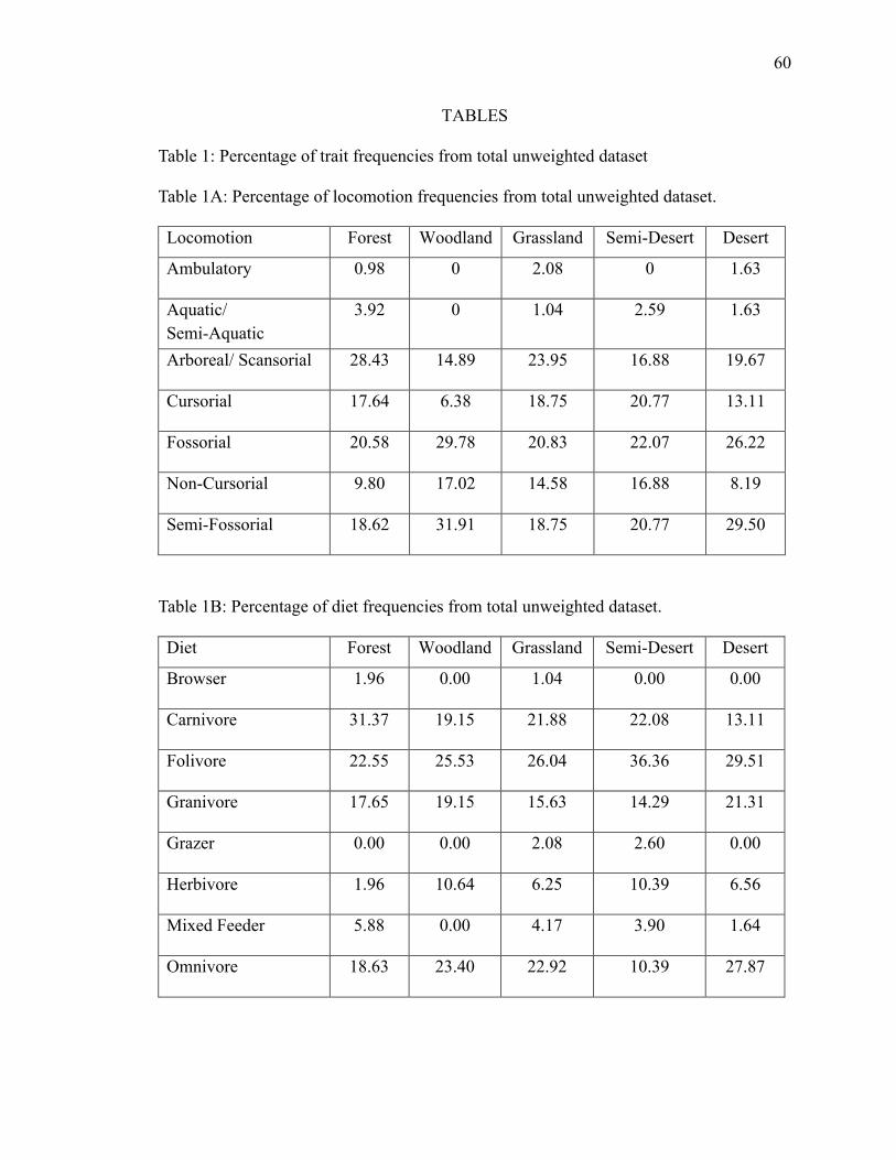
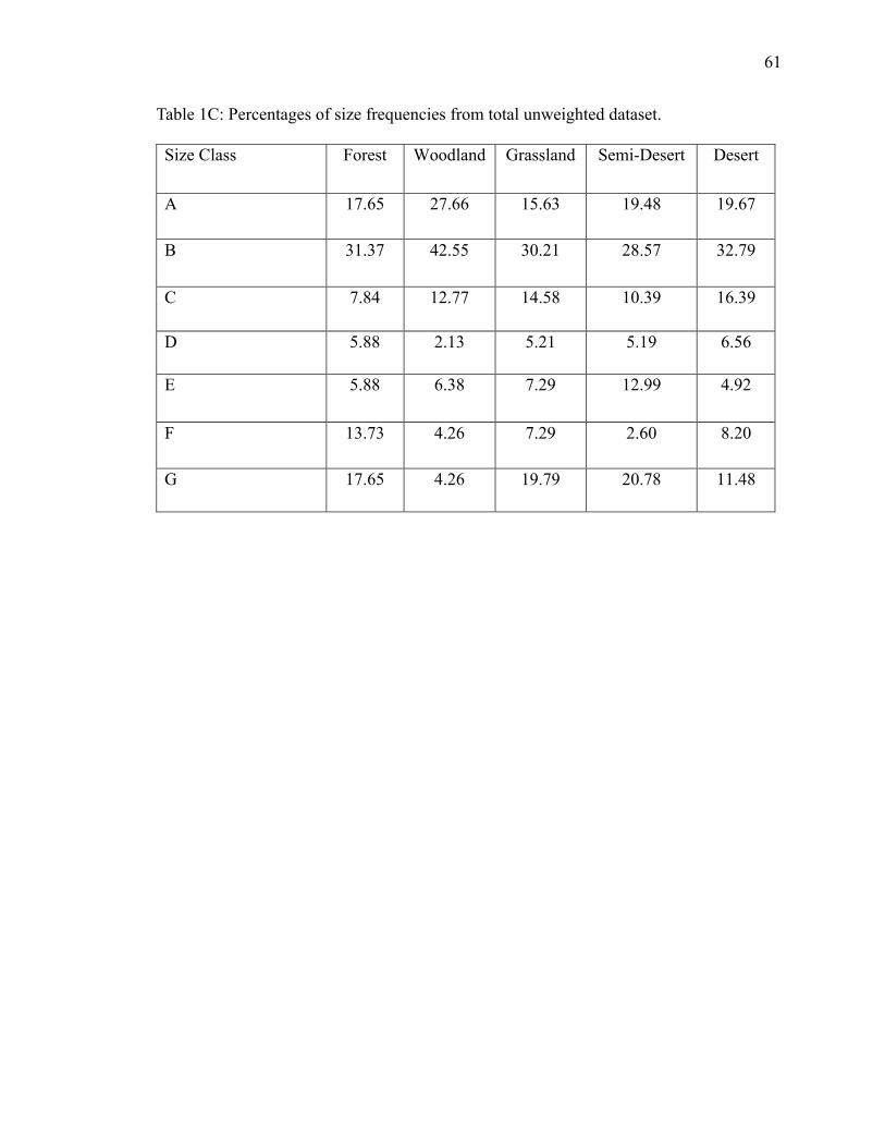
1. Table 1: Percentage of trait frequencies from total unweighted dataset……….........60

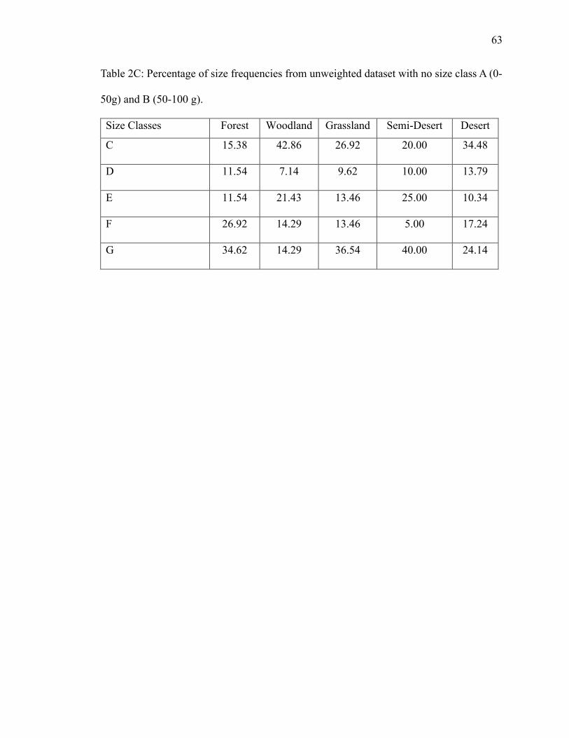
2. Table 2: Percentage of trait frequencies from total unweighted dataset with no size

class A and B……………………………………………....………………………....62

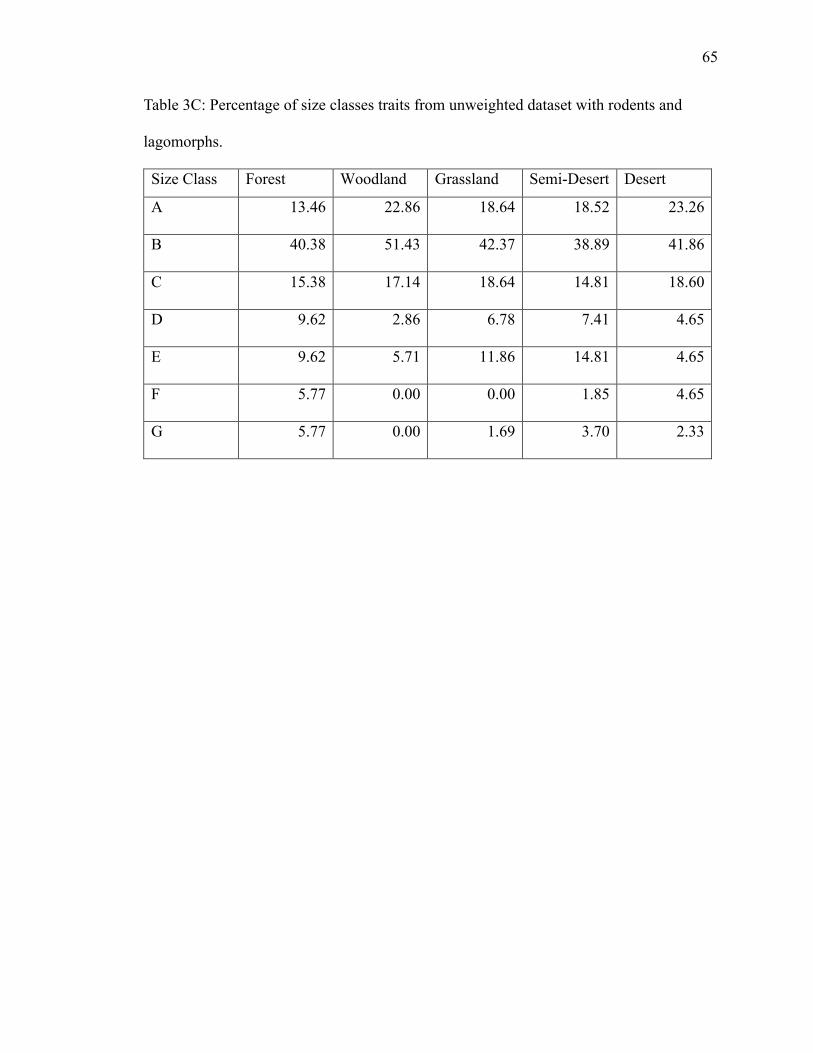
3. Table 3: Percentage of trait frequencies from total unweighted dataset with rodents

and lagomorphs…………………...………………………………………………….64

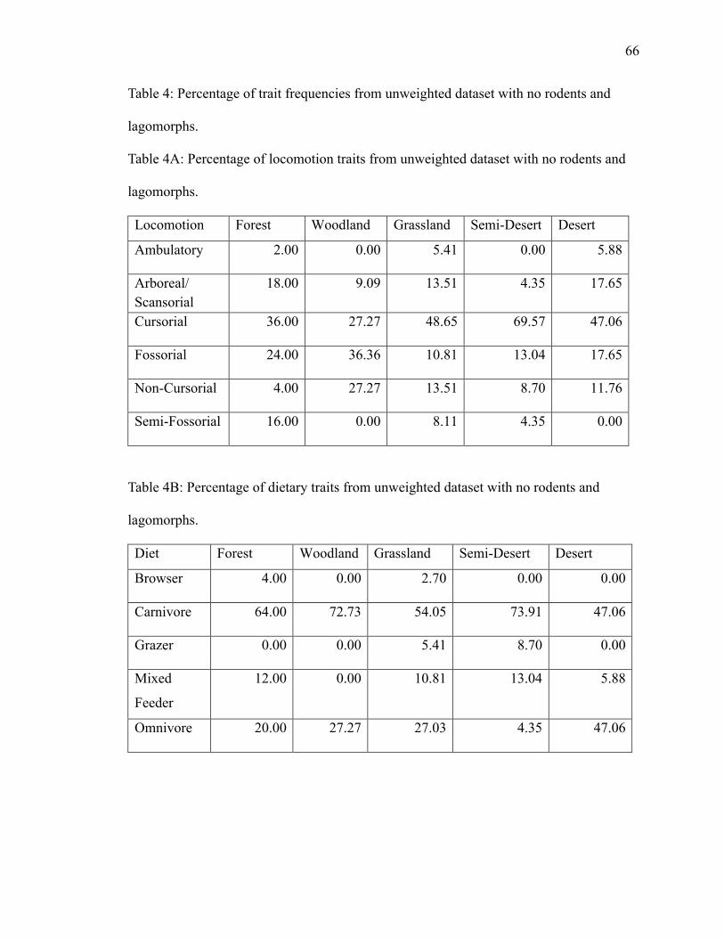
4. Table 4: Percentage of trait frequencies from total unweighted dataset with no rodents

and lagomorphs ……………………………………………………………...………66

5. Table 5: Percentages of trait frequencies from total weighted dataset……………….68

6. Table 6: Percentages of trait frequencies from weighted dataset with no size class A

and B………….………….…………………………………………………………..70

7. Table 7: PCA loadings of all trait frequencies from unweighted dataset with no size

classes A & B………………………………………………………………………...72

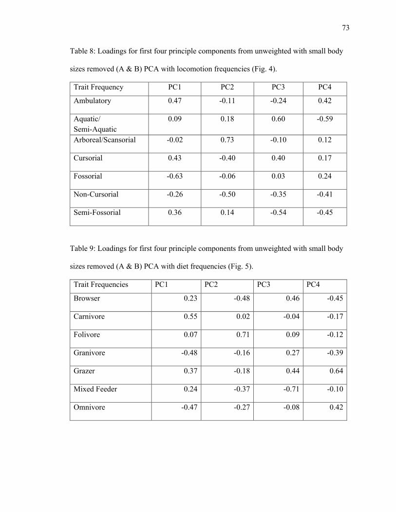
8. Table 8: PCA loadings of locomotion trait frequencies from unweighted dataset with

no size classes A & B………….……………………………………………………..73

9. Table 9: PCA loadings of diet trait frequencies from unweighted dataset with no size

classes A & B………………………………………………………………………...73

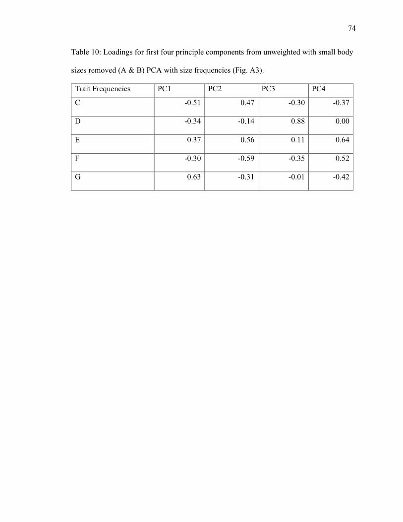
10. Table 10: PCA loadings of size trait frequencies from unweighted dataset with no size

classes A & B………………………………………………………………………...74

11. Table 11: PCA loadings of all trait frequencies from weighted dataset with no size

classes A & B………………………………………………………………………...75

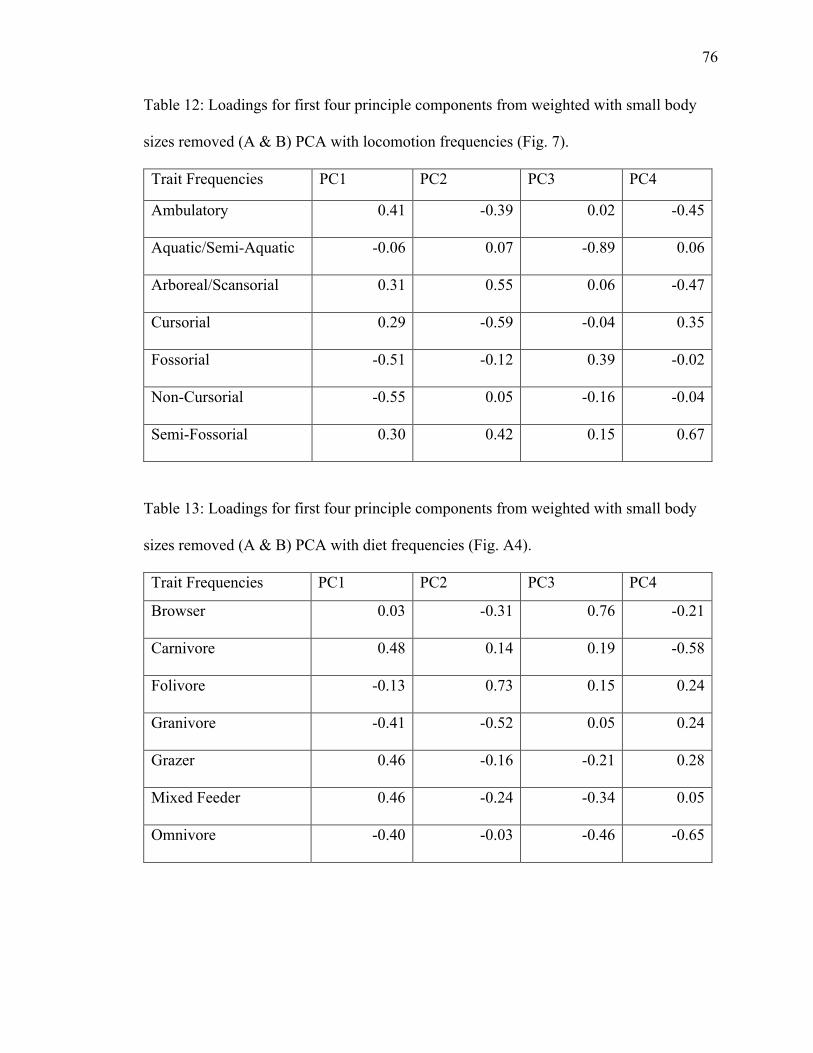
12. Table 12: PCA loadings of locomotion trait frequencies from weighted dataset with

no size classes A & B………………………………………………………………..76

ix

13. Table 13: PCA loadings of diet trait frequencies from unweighted dataset with no size

classes A & B………….……………………………………………………………..76

14. Table 14: PCA loadings of size trait frequencies from unweighted dataset with no size

classes A & B………….……………………………………………………………..77

15. Table 15: PCA loadings of all trait frequencies from total unweighted dataset……...78

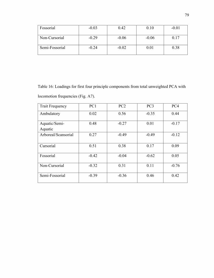
16. Table 16: PCA loadings of locomotion frequencies from total unweighted dataset…79

17. Table 17: PCA loadings of diet frequencies from total unweighted dataset...……….80

18. Table 18: PCA loadings of size frequencies from total unweighted dataset…………80

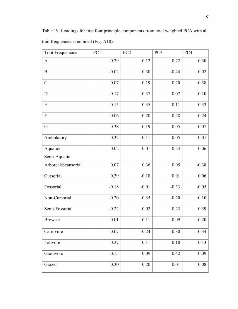
19. Table 19: PCA loadings of all trait frequencies from total weighted dataset………...81

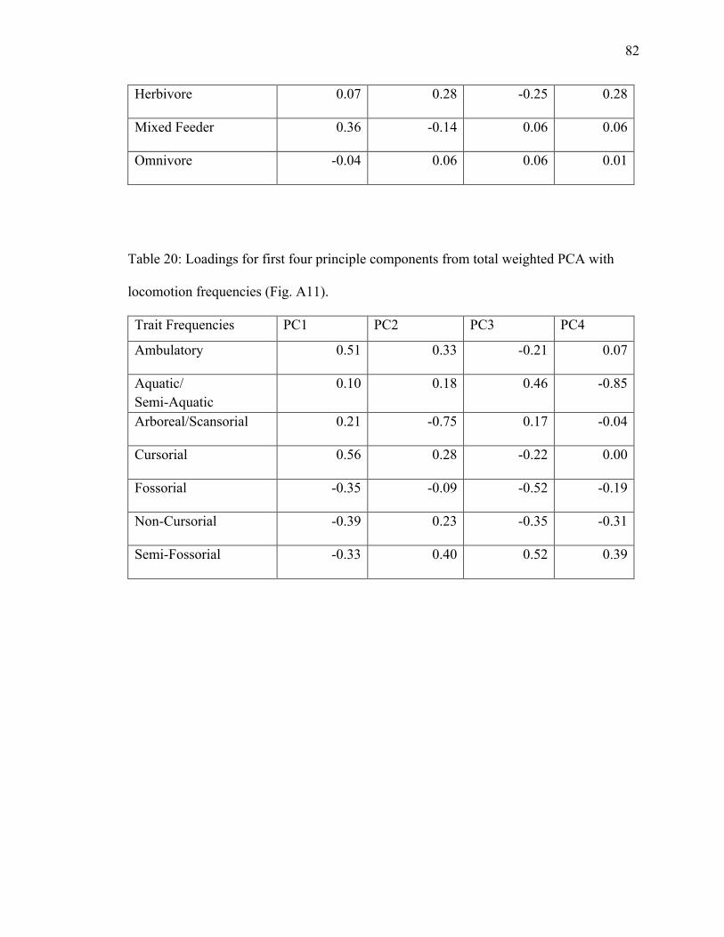
20. Table 20: PCA loadings of locomotion frequencies from total weighted dataset…....82

21. Table 21: PCA loadings of diet frequencies from total weighted dataset…................83

22. Table 22: PCA loadings of size frequencies from total weighted dataset……………83

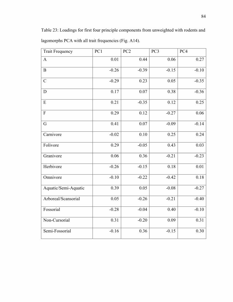
23. Table 23: PCA loading scores of all trait frequencies from unweighted with rodents

and lagomorphs………….………….………….…………………………………….84

24. Table 24: PCA loading scores of all trait frequencies from unweighted with no

rodents and lagomorphs ………….………….………….………….………………..85

x

LIST OF FIGURES

1. Figure 1: Size frequency distribution of original North America taxa ……………...86

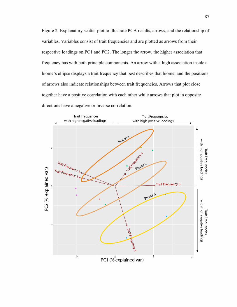
2. Figure 2: Explanatory scatter plot of PCA…………………………………………...87

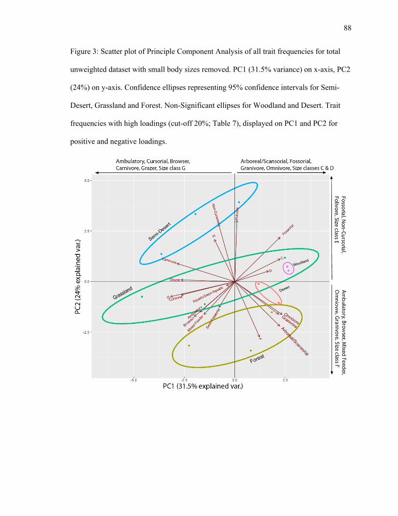
3. Figure 3: Scatter plot of PCA with all trait frequencies for total unweighted dataset

with no size classes A & B…………………………………………………………...88

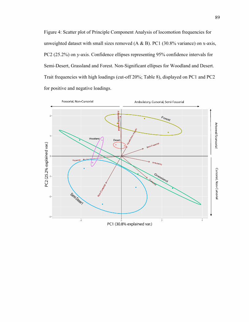
4. Figure 4: Scatter plot of PCA with locomotion frequencies for total unweighted

dataset with no size classes A & B…………………………………………………...89

5. Figure 5: Scatter plot of PCA with diet frequencies for total unweighted dataset with

no size classes A & B………………………………………………………………...90

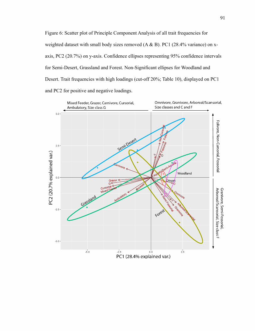
6. Figure 6: Scatter plot of PCA with all trait frequencies for total weighted dataset with

no size classes A & B………………………………………………………………...91

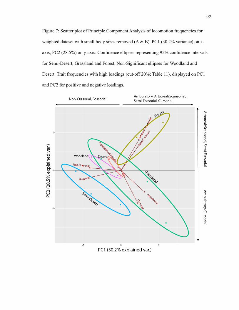
7. Figure 7: Scatter plot of PCA with locomotion frequencies for total weighted dataset

with no size classes A & B…………………………………………………………...92

8. Figure 8: Stacked area charts for trait frequencies in total unweighted

dataset………….…………………………………………………………………….93

9. Figure 9: Stacked area charts for trait frequencies in total unweighted dataset with no

size classes A & B……………………………………………………………………94

10. Figure 10: Stacked area charts for trait frequencies in total weighted dataset…….....95

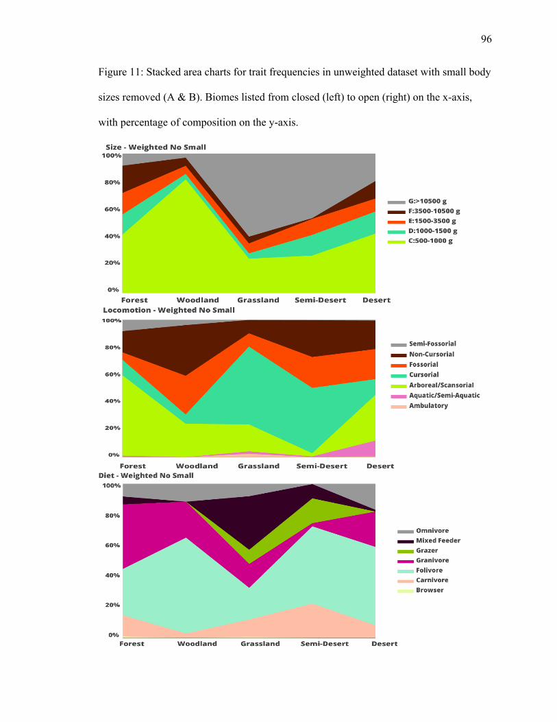
11. Figure 11: Stacked area charts for trait frequencies in total weighted dataset with no

size classes A & B………….………………………………………………………...96

1

1. INTRODUCTION

In its broadest sense, the goals of paleoecology are to understand how ancient

organisms interacted, and the kinds of habitats and biomes that were present where these

organisms lived. Various proxies have been used to reconstruct ancient environments,

such as stable carbon isotopes, soil types, sedimentary facies, and the compositions of

fossil floras and fossil faunas (e.g., Edwards et al. 2010; Feranec 2007; Secord et al.

2008; Ehleringer et al. 1991). Key functional traits in vertebrates that have been shown to

be correlated with environmental variables are sometimes used. For example, the

frequency of hypsodonty (tooth crown height) in mammal species is significantly

correlated with precipitation, with a higher percentage of hypsodont species in dry areas

(Polly et al. 2011; J. T. Eronen, Polly et al. 2010). Although this approach is useful, it

often serves to infer only one aspect of the environment. Broader approaches have also

been employed that involve various functional aspects of an entire faunal community, or

the frequencies of these aspects within the community (e.g., Andrews and Hixon, 2014).

An example of this approach is the frequency of grazing (grass-eating) and browsing

(leaf-eating) species in a mammal fauna. Grazers would be expected to occur in higher

frequencies than browsers in grasslands, and the inverse in forests, based on modern

analogs (Cerling & Harris 1999). This “community ecology” approach relies on the

assumption that functional traits, which are physical adaptations that serve a specific

function in an organism's environment (Polly et al. 2011), can be used to glean

information about ancient environments. Functional traits in mammals generally occur in

three ecological categories: locomotion, diet, and body mass. By analyzing the

distribution of traits within these categories, paleoecological models can be developed for

2

interpreting past environments (e.g., Andrews and Hixon, 2014). Because the range of

trait distributions in modern mammals is directly related to their respective environments,

interpretations of past ecosystems are possible (Pineda-Munoz & Alroy 2014; Andrews

& Hixson 2014).

As one goes further back in time the assumption that a taxon retains the same

ecological niche becomes increasingly tenuous (Secord et al. 2008). Thus, it is desirable

to use “taxon-free” community approaches when possible. Analyzing the frequency of

traits within a community can be done without taxonomic consideration based on the

assumption that these traits are adapted to a specific ecological niche independent of

phylogeny. However, an organism’s phylogenetic history imposes constraints on the

adaptability of that organism (e.g., Barnosky et al. 2001; Brooks and McLennan 1993;

Losos 1996; Jablonksi and Sepkoski 1996; Ricklefs 2007), and it is doubtful that any

approach is truly taxon free (e.g., see Andrews and Hixon, 2014). Nevertheless, the

ability to directly study traits and trait distributions, instead of species, minimizes

inherent taxonomic bias when applying modern observations to fossil communities. In

order to identify traits useful for making both ecological and paleoecological

interpretations, it is important to understand the processes controlling the relationship

between these traits and associated environmental conditions.

The objective of this thesis is to develop a comprehensive model for interpreting

Neogene biomes in North America. I explore the efficacy of several multi-proxy

paleoenvironmental models based on the frequency of trait distributions in locomotion,

diet, and body mass in modern mammalian communities. While many previous proxies

have been developed from African or European ecosystems, there is a high potential for

3

error when regionally-derived proxies are applied globally (e.g., P. J. Andrews, Lord, and

Evans 1979; P. Andrews and Hixson 2014; Meloro 2011; Plummer, Bishop, and Hertel

2008; Rodríguez 2004; Rodriguez, Hortal, and Nieto 2006; Van Valkenburgh 1988).

Additionally, no model is completely taxon-free, and phylogenetic influences cannot be

entirely discounted. For these reasons the models I develop are based on modern and

historical North American faunas, rather than Old World faunas. Also, many studies that

use mammalian traits as proxies exclude small-bodied mammals or group them with

larger mammals (e.g., Liu et al. 2012; J. Eronen, Puolamäki, and Liu 2010; J T Eronen et

al. 2010; Rodríguez 2004; P. Andrews and Hixson 2014; Soligo and Andrews 2005;

Legendre 1986). There is a significant collection bias against small-bodied mammals in

African-based proxies, and the implications of this bias on paleoecological interpretations

are not fully understood (Soligo & Andrews 2005; Damuth & Janis 2011; Andrews &

Hixson 2014). Hence I explore the impact that small-bodied mammals have on

distinguishing biomes in the model. I also examine the impact of weighting traits by the

number of geographic occurrences of a taxon, versus using only a single occurrence in

each biome. Furthermore, I explore the differences between taxon-free and phylogenetic

analyses by combining the unweighted dataset into two groups, rodents and lagomorphs,

and all remaining taxa. Lastly, I compare models built for this study with some published

models. Results of this study indicate which community models are best suited for

paleoecological interpretations in North America and build the foundation for future

Neogene paleoecological studies.

4

2. BACKGROUND

Research conducted by Andrews et al. (1979) provided much of the groundwork

for subsequent studies of community ecology that examine mammalian traits and their

relationship to the environment. Andrews, et. al focused on describing biomes solely on

trait assemblages and applying those modern ecological relationships to the fossil record.

Biomes, as used here, are broad, regional areas that share similar environmental factors

(Bailey 1983), whereas habitats describe local conditions where an organism or

community lives (Odum 1959). Andrews, Lord, and Evans divided extant African

mammal communities into five general biomes: lowland forest, montane forest,

woodland-bushland, grassland, and floodplain. They classified extant mammals by diet

(carnivore, insectivore, grazers, browsers, frugivores, omnivores), size (< 1 kg, 1-45

kg, >45 kg), locomotion (aerial, arboreal, scansorial, terrestrial, fossorial, aquatic), and

taxonomic groups (rodents and insectivores, primates, artiodactyls and carnivores)

(Andrews et al. 1979). By analyzing the range of functional traits in each group, they

created trait indices, which they subsequently applied to fossil communities. Three

modern biomes had unique indices: forest, woodland-bushland, and grassland. These

indices allowed for the interpretation of two (out of five) fossil communities as forest and

woodland biomes (Andrews et al. 1979). This study demonstrated that modern biomes

could be classified using the distribution of traits within mammalian communities, and

these relationships can be used for paleoecological interpretations.

More recent research has been focused on developing taxon-free approaches,

which has met with mixed success. One such example is the study of ecomorphological

(or ecometric) traits, which are functional traits directly related to the ecosystem, of

5

extant African mammals by Andrews and Hixson (2014). They used body mass,

locomotion, and diet as ecological categories, because these represent distinct divisions

within communities: an organism's size, the space it occupies, and its trophic level. Their

research focused on determining how well biomes can be distinguished by

ecomorphological traits. Body mass did not show clear trends among the biomes and was

determined to be the least useful category (Andrews & Hixson 2014); it is also not

entirely taxon-free (e.g., rodents and lagomorphs have clear limits to maximum size).

Regressions for calculating body mass are based on higher taxonomic groupings, and

different clades exhibit different ranges for body mass (e.g., Legendre 1986), creating

inherent bias within body mass metrics. Locomotion and diet, on the other hand, each

showed clear differentiation among biomes, supporting the hypothesis that morphological

traits can be used to infer biomes (Andrews & Hixson 2014). Building on prior ecological

foundations (e.g., J T Eronen et al. 2010; Polly et al. 2011; Soligo and Andrews 2005),

this research was a prime example of the “taxon-free” concept in paleoecological studies.

Dietary classifications can be used to analyze geographic differences in diet

diversity among mammals. For example, Badgley and Fox (2000) related the locations of

species to environmental and physiographic factors. They placed species in spatial

quadrants across North America and analyzed the diversity of species’ body sizes and

diet classifications to establish thresholds (Badgley & Fox 2000). Results showed that

species with smaller body sizes had higher diversity at lower latitudes, whereas species

with larger body sizes exhibited higher diversity at higher latitudes. Furthermore, species

diversity in frugivores, omnivores, granivores, and aerial insectivores, as well as those

with the smallest body sizes (< 1kg), was affected by gradients in both temperature and

6

moisture. Aerial insectivores, frugivores, and terrestrial invertivores are also more diverse

at lower latitudes. The diversity of species with medium to large body sizes increased

from east to west, along with diversity of granivores and herbivores (Badgley & Fox

2000). This study showed geographic trends in both diet and body size, and their

relationship to abiotic factors.

Pineda-Munoz et al. (2016) studied the relationship between diet and body mass

in modern mammals. They grouped extant mammals into eight dietary categories based

on stomach content data: herbivore, carnivore, frugivore, granivore, insectivore,

fungivore, gumivore, and generalized. Pineda-Munoz et al. observed a significant

separation of diets in mammals smaller than 1 kg and mammals larger than 30 kg using

Principle Component Analyses (PCA). Smaller mammals had the largest diet diversity,

encompassing insectivores, granivores, and mixed feeders, whereas large mammals had a

narrow range of diets, including only carnivores and grazers. The medium-sized

mammals (1-30 kg) consisted primarily of frugivores (51.55), while 75% of frugivores

were placed in the medium size range. Frugivores were found to be the most distinct

dietary group, with a significant body mass difference between frugivores and granivores,

insectivores, and generalists (Pineda-Munoz et al. 2016). Frugivores had the third largest

sample size (insectivore and herbivore with more), but the size range for the medium size

bin was quite broad (1 kg to 30 kg). When applied to fossil assemblages, Pineda-Munoz

et al. indicated that keeping dietary categories separate is most appropriate. For

paleoecological interpretations conducted with both dietary categories and body sizes as

proxies, combining diet categories may mask environmental factors (Pineda-Munoz et al.

2016). However, differentiating dietary groups can be difficult for fossil taxa. Diet is

7

interpreted from dental morphology, microwear, or stable carbon isotopes, but these

proxies do not always match dietary categories in modern taxa, and all are not useful for

the full dietary range observed in modern mammals (e.g., J. Eronen, Puolamäki, and Liu

2010; Liu, Puolamaki, et al. 2012; Evans et al. 2007; Cerling et al. 2003; Secord, Wing,

and Chew 2008; Feranec 2007). This study demonstrated the relationship between

ecometric categories and highlighted potential problems in paleoecological applications.

Additional research on the connection between body size and diet has

demonstrated their interconnectedness. Price and Hopkins (2015) investigated large-scale

ecological patterns in mammals by combining diet and body size data with a

phylogenetic analysis. Dietary groups were broad: herbivore, carnivore, and omnivore.

Using generalized Ornstein–Uhlenbeck phylogenetic models, Price and Hopkins (2015)

showed a macroevolutionary relationship between diet and body size in mammals. They

observed that terrestrial omnivores were generally larger than carnivores, and terrestrial

herbivores were larger than omnivores. Rodents deviated from the general trend and

separate patterns were displayed. Within the carnivore dietary group, rodents displayed a

higher body mass, while omnivores displayed a lower body mass. Carnivorous rodents

were not the majority in the data, as 21 of the 409 rodent species were classified as

carnivores, and 11 of those rodent species were semi-aquatic with a diet of fish, crabs,

and aquatic snails. Price and Hopkins (2015) concluded that the carnivorous preferences

of these larger rodents potentially reflected that available prey increases with body mass.

Research highlighting the relationship between phylogenetic evolution and ecometric

traits suggests that ecometric traits are interconnected within and outside phylogenetic

8

clades. Price and Hopkins' research also suggests there is an inherent taxonomic presence

in all ecometric studies.

In addition to both body size and diet analyzed together and separately, the

relationship of locomotion and the environment has primarily been studied in isolation.

Locomotion is often used to determine the openness of an environment (Polly 2010). In

carnivores, highly digitigrade mammals are associated with open environments, such as

prairies, steppes, or deserts, while plantigrade mammals are associated with closed

environments including woodlands or forests (Polly 2010). Taxon-free approaches rely

on the convergence of traits across phylogenetic classifications. Locomotion is a prime

example of that convergence. Locomotion is primarily based on morphology of a species,

and convergent morphology occurs when different species live in similar habitats (e.g.,

Jenkins and Camazine 1977; Alexander et al. 1979; Brown and Yalden 1973;

Christiansen 1999; J. M. Smith and Savage 1956). Samuels et al. (2013) examined the

range of locomotion within Carnivora, including both extant and extinct taxa of North

American families that are not closely related: Amphicyonidae, Barbourfelidae, Canidae,

Felidae, Miacidae, Mustelidae, Nimravidae, and Ursidae. They used 20 osteological

measurements to determine locomotor habit and included extinct carnivores with no

modern morphological analog. Locomotion was split into six groups: terrestrial,

cursorial, scansorial, arboreal, semi-fossorial, and semi-aquatic. Both morphological

indices and locomotor groups were found to be convergent for extant and extinct taxa.

Cursorial and terrestrial hyaenids, canids, and felids all had relatively elongate and

gracile limbs and grouped together; semi-fossorial mephitids and badgers also grouped

together. The morphological indices were found to best discriminate cursorial and

9

arboreal species. In addition, species with similar locomotor groups converged towards

similar morphology, regardless of the level of phylogenetic relationship (Samuels et al.

2013).

Meloro (2011) reconstructed locomotor behavior of Italian Plio-Pleistocene

carnivore families by using long-bone metrics of extant and fossil species. He used 22

extant species of Canidae, Felidae, Hyaenidae, and Ursidae, accounting for phylogenetic

relatedness since closely related species tend to have similar behavioral and

morphological traits (Meloro 2011). He restricted modern carnivores to large taxa (>7kg)

with a well-researched fossil record on the Italian peninsula and used related modern taxa

to assign locomotor behavior to fossil taxa. Meloro (2011) found in a PCA of extant and

extinct taxa that locomotor behavior and long bone measurements indicated general

patterns of association between extinct carnivores and their habitat. Meloro (2011) found

that carnivores were not habitat specialists, unlike ungulates and rodents. Instead,

carnivores have large home ranges, and their habitat selection is dependent on the density

of prey and other predators. Carnivores may be well adapted to specific habitats but will

select sub-optimal habitats when pressured from external factors (Meloro 2011). The

results of Samuels et al. (2013) and Meloro (2011) show that ecometric traits can be

convergent, supporting the viability of taxon-free approaches.

While the relationship among ecometric traits is essential, understanding the

relationship between mammalian body mass and the environment is equally necessary.

Rosenzweig (1968) examined the influence that environmental factors have on body

mass in modern mammalian carnivores. Temperature and latitude were suggested to

represent measures of the same environmental pressure on body size (Rosenzweig 1968).

10

He found that body size for the female marten and male coyote, as well as both sexes of

the red fox, gray fox, badger, and ermine, could be predicted by both temperature and

latitude. Evapotranspiration also predicted body size in water-stressed and/or heat-

stressed environments (Rosenzweig 1968). Furthermore, Rosenzweig (1968) observed a

connection between diet and body size, concluding that a carnivore’s body size is

dependent on both prey size and the frequency with which it can obtain prey. Thus, large

Carnivora taxa (e.g., bears) take in a high amount of vegetation when hunting smaller-

sized prey that are not readily available, choosing an omnivorous diet rather than a

carnivorous one. The results of Rosenzweig (1968) show the interconnectedness of body

size and the environment, and the relationship between environmental factors and body

size.

11

3. METHODS

3.1 North American Modern Mammal Database

To compile a database of modern mammal trait frequencies in North America, I

downloaded a list of North American mammals from NatureServe Explorer (NatureServe

2016) and species field guides from the Smithsonian North American Mammals database

(Smithsonian National Museum of Natural History). I removed the families Chiroptera,

Sirenia, Cetacea, Odobenidae, and Otariidae to ensure the database included species that

are native to North America and either non-marine aquatic, non-marine semi-aquatic, or

terrestrial. This initial list totaled 537 species.

For each species in the modern North American list, I compiled data on body size,

diet, and locomotion from a variety of sources. My primary source was NatureServe's

online searchable database (NatureServe 2016). I supplemented body mass measurements

from PanTHERIA (Jones et al. 2009), Quaardvark (University of Michigan Museum of

Zoology 2013), and Wilman et al. 2014, and calculated averages for each species. I

assigned taxa to body mass ranges ("Body Class"), giving a letter to each range: A (0-50

g), B (50-500 g), C (500-1,000 g), D (1,000-1,500 g), E (1,500-3,500 g), F (3,500-10,500

g) and G (>10,500 g) (Table A1c). To determine the body mass classes, I created a

frequency histogram (Fig. 1) using the ‘PivotTable' and ‘Histogram' analyses functions in

Excel 2016 (Microsoft Office 2016). While a clear bias towards smaller body masses is

evident, distribution of body mass above 500 g remains even. I initially assigned diet and

locomotion from NatureServe's previous designations and their description of each

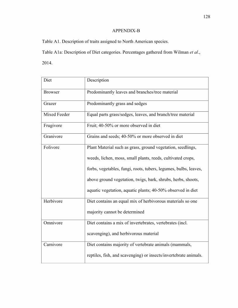
species' recorded diet (Table A1a, A1b). I then refined the diet categories with stomach

content percentages from Wilman et al. (2014). Locomotion data were validated and

12

refined with Walker's Mammals of the World 6th ed. (Nowak 1999a; Nowak 1999b).

Dietary categories are: carnivore, omnivore, frugivore, granivore, folivore, browser,

grazer, mixed feeder, and herbivore (Table A1a). Here, carnivore is defined as consuming

vertebrate and/or invertebrate animals, and omnivore is defined as consuming a mix of

invertebrates, vertebrates, and plant material. Frugivore is defined as consuming fruit

material, and folivore is defined as consuming plant material, such as grass, ground

vegetation, weed, moss, lichen, twigs, bark, and leaves (see Table A1b for frequencies).

Folivore is used only for non-ungulate mammals. Grazer (grass and sedges), browser

(leaves and branches), and mixed feeder (grass and tree material) are assigned to ungulate

mammals. Herbivore is defined as diets with an equal mix of either folivore, granivore,

and frugivore. Locomotion frequencies are ambulatory, aquatic/semi-aquatic,

arboreal/scansorial, cursorial, fossorial, non-cursorial, semi-fossorial (Table A1b).

Terrestrial locomotion traits are ambulatory (defined as exhibiting plantigrade

morphology), cursorial (defined as having digitigrade or unguligrade morphology), and

non-cursorial (neither plantigrade, digitigrade, or unguligrade morphology).

Aquatic/semi-aquatic groups both aquatic and semi-aquatic locomotion habits in one

category due to low numbers of each when separated. Arboreal/scansorial is defined as

the ability to readily climb trees (e.g. squirrels). Semi-fossorial is defined as spending

active time on the ground surface and in burrows, and inactive time in burrows. Fossorial

is defined as spending both active and inactive time in burrows. In cases where

locomotion data were missing from available sources (Quaardvark, PanTHERIA,

Wilman et al. 2014, NatureServe, and Walker's Mammals of the World), those species

13

were assigned as "Unknown". Species with unknown locomotion classification totaled

52, all consisting of rodents and shrews from understudied regions of Mexico.

3.2 Historical Database

Historical occurrence data were downloaded from the American Museum of

Natural History's (AMNH) Online Mammalogy Database (American Museum of Natural

History 2018). Searches used the original list of 537 species from the modern North

American database, searching each family, genus, or species for localities in the United

States, Mexico, and Canada. I trimmed the database to include only records collected

before 1900 to reduce the potential for human disturbance. Historical occurrence data, as

opposed to recent occurrences, were used to create a biome database that represented

ecosystems that were less disturbed by humans. I also removed records with no

associated date, records without county-level locality data, and records of island

occurrences.

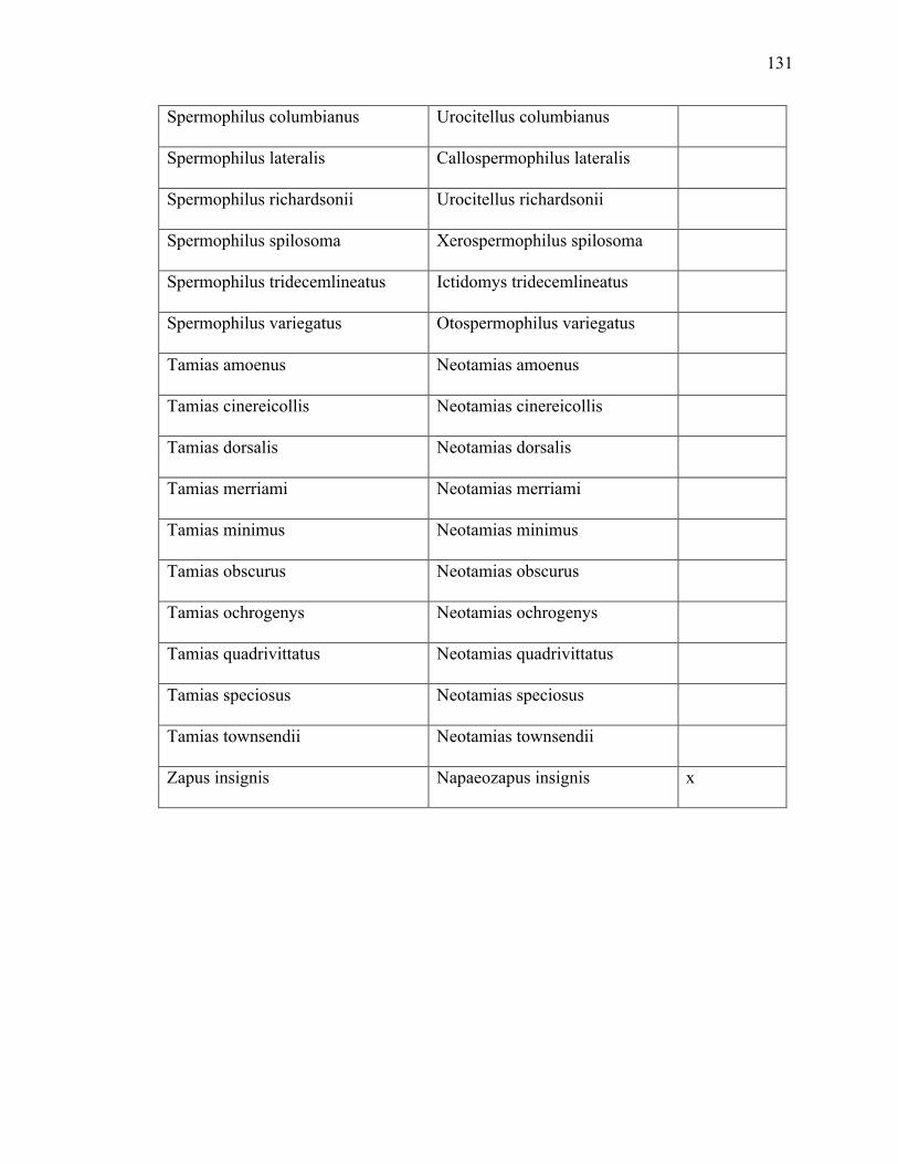
Next, taxonomic names were updated in the historical database to reflect changes

in taxonomy. Taxonomic duplicates or discrepancies were observed mainly in rodents

and shrews, as taxonomical reorganization has resulted in species being moved among

genera, or changed from sub-species to species. I downloaded a significant proportion of

the occurrence data using family or genus search queries, thus there is potential for

taxonomic discrepancies. If there was overlap between old and new species names, I used

the most current taxonomic nomenclature following Nowak (1999a;1999b), (Table A2).

Frequency data for locomotion, diet, and body mass were brought in from the modern

North American database. Historical species totaled 135 after correcting for taxonomy.

The final historical database with associated biomes consisted of 8240 occurrences.

14

Both a weighted and unweighted dataset were created from the historical data.

Faunas with only a few dominant taxa that are abundant throughout a biome are not

accurately represented by unweighted data that do not account for number of

occurrences. For example, bison occur with a very low frequency in the taxonomic list,

but historically had high abundances where they occurred. There are very few grazers in

the historical dataset, and including their abundances in the analyses could yield patterns

that otherwise were masked. Additionally, the unweighted dataset was split into two

groups for taxonomic analyses: rodents and lagomorphs, and all other taxa.

After finalization of the historical database, I plotted each occurrence record using

Google Earth Pro (Google Earth Pro, 2018) by adding a placemark in the center of the

observed county for each record. I saved these placemarks as a .KMZ file and imported

into ESRI ArcMap 10.4.1 (ArcGIS 10.6).

3.3 Biome Assignment

I downloaded Bailey's Ecoregions of North America map (Fig. A1) from the

United States Department of Agriculture Forest Service Rocky Mountain Research

Station's website (Rocky Mountain Research Station 1996) and used it in conjunction

with the AMNH historical data. In ArcMap, I combined the Ecoregions of North America

map and AMNH historical occurrence data (ArcToolbox; Overlay; Analysis Tools;

Spatial Join) (Rocky Mountain Research Station 1996). This allowed each occurrence to

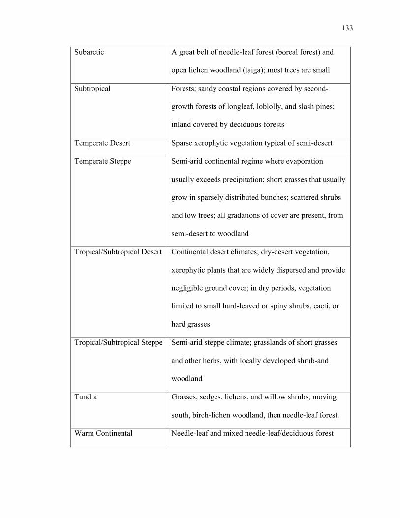
be assigned geographical ecoregion data. I kept the names of Bailey's Division

ecoregions (Table A3) the same except for the ‘Marine’ Division ecoregion, renaming

them as ‘Coastal’ as to avoid confusion about the terrestrial nature of the biomes. Bailey's

ecoregions were re-assigned to broader biomes (Table A4) after preliminary Principle

15

Component Analyses (PCA). Temperate and precipitation ranges and averages of

Divisions, along with Divisions consistently plotting together (i.e., Tropical/Subtropical

Steppe and Prairie; Temperate Desert and Temperate Steppe) were used to group the

divisions into the broad biomes. I used Bailey's Ecocodes to test variability in each

biome. Ecocodes are numerical representations of Bailey’s Divisions (Bailey 1995), and

each biome contains multiple ecocodes that serve as sub-sampling points. To avoid

including under-sampled local faunas, only sub-samples with sizes greater than 35% of

the total taxa in the biome were used. Sub-samples of 35% or greater were found to best

represent the community structure and recorded habitat (Andrews & Hixson 2014). Most

sub-sample points have a higher percentage of taxa, ranging from 40% to 95%; however,

there are a few points with 30%. Extreme habitats (Rainforest, Savanna, Subarctic, and

Tundra) and all mountainous regions, which were clearly outside the range of understood

North American Neogene habitats, were excluded to better tailor the model for Neogene

applications. The final historical data distribution is displayed in Figure A2.

3.4 Statistical Analysis

I used RStudio (RStudio, Version 1.0.143; R Version 3.4.3) for statistical

analyses. I used packages "Plotly" (Plotly, Version 4.7.1) and "Ggplot2" (Ggplot2,

Version 2.2.1) to create plots and graphics, and "RSelenium" (RSelenium, Version 1.7.1)

to export graphics into ‘.svg' files. I created figures in Adobe Illustrator CC (Adobe

Creative Cloud, Illustrator Version 22.1). All analyses were conducted with the historical

taxa list and associated trait frequencies. All RStudio script is included in Appendix-A.

I imported two sets of data into RStudio: historical unweighted data (one taxon

per biome) and historical weighted occurrence data (includes number of recorded

16

occurrences per biome). For each set of data, a new data frame was created, and new

columns were then added for each of the individual biomes, with presence and absence

data for each biome by row. Then, taxa were separated by trait, and the number of

presences per biome were totaled. Tables were made for the proportion of trait

classifications in each biome. Cumulative stacked proportions (totaling 100%) were also

created for stacked area charts for each trait per biome, with the biomes arranged on the

x-axis from closed (right) to open (left) (Appendix-A M1). Stacked area charts were used

to analyze the composition of each trait frequency across biomes.

I conducted PCAs using trait frequencies expressed as percentages of the total

traits per category (i.e., diet, locomotion, body mass) for each biome. For example, diet

for the unweighted dataset in the grassland biome consists of 22.9% omnivores, 2.1%

grazers, etc. For the analyses, I brought in Bailey's ecocodes (Rocky Mountain Research

Station 1996) to ensure a sub-sampling within biomes (Appendix-A M2). Sub-sampling

created 13 total data points in all PCA diagrams. Forest, grassland, and semi-desert all

had three sub-sampling points, while woodland and desert each had two. I plotted

confidence intervals onto the PCA plots for each biome with three subsampling points

(Appendix-A M3). These were calculated assuming a normal, multi-variate distribution

and with a 95% confidence level. Due to low sub-sample size, woodland and desert do

not have 95% confidence ellipses plotted. In total, I used six datasets: unweighted (Table

1), unweighted without size classes A (0-50 g) and B (50-500 g) (Table 2), unweighted

rodents and lagomorphs (Table 3), unweighted without rodents and lagomorphs (Table

4), weighted (Table 5), weighted without size classes A and B (Table 6). Each dataset

was analyzed with all traits combined, and also separately with locomotion, diet, and

17

size. From the historical species list, 33 species weigh less than 50 g (24% of the total

species list), and 46 species weigh between 50 and 500 g (34%). Removing both size

classes A and B removed 51% of the unweighted dataset and 64.5% of the weighted

occurrence dataset. Rodents and lagomorphs make up 44.7% of the unweighted data. I

repeated the analyses four times per dataset, one with all the traits combined, and one for

locomotion, diet, and size separately. For the taxonomically grouped data, analyses were

only conducted on the traits combined. Removing size classes A and B created a

weighted dataset of 2348 occurrences and an unweighted dataset of 187. Analyses were

additionally conducted with and without rodents and lagomorphs for the unweighted data.

Rodents and lagomorphs created an unweighted dataset of 243 taxonomic occurrences

and the remaining taxa created a dataset of 138.

18

4. RESULTS

4.1 Principle Component Analysis

PCA diagrams consist of PC1 on the x-axis, and PC2 on the y-axis. Sub-sampling

points and confidence ellipses for each biome (with n=3) are plotted using the scores of

each point for the two principle components. Thirteen points were plotted in total,

representing the five biomes. An explanatory PCA (Fig. 2) illustrates arrows and the

relationships of variables. Variables consist of trait frequencies and are plotted as arrows

from their respective loadings on PC1 and PC2. The longer the arrow, the higher

association that frequency has with both principle components. In Figure 2, trait

frequency 3 has a high association with PC1 and trait frequency 5 has a high association

with PC2. Conversely, the shorter the arrow, the lower association, as seen in trait

frequency 4 in the explanatory figure (Fig. 2). An arrow with a high association inside a

biome’s ellipse displays a trait frequency that best describes that biome (trait frequency 5;

Fig. 2). The positions of arrows also indicate relationships between trait frequencies.

Arrows that plot close together have a positive correlation with each other (trait

frequency 1 & 2; Fig. 2), while arrows that plot in opposite directions have a negative or

inverse correlation (trait frequency 1 & 3; Fig. 2). Trait frequencies with loadings 20% or

higher are displayed on the figures, outside the plotting area (Fig. 2).

For the sake of brevity, PCA plots that show the greatest separation among

biomes are shown in the main text, while those with poor separation are included in the

appendix (Appendix-C).

19

4.1.1.1 Unweighted Diet, Locomotion, Medium & Large Body Size (≥500 g) PCA

PC1 explains 31.5% of variance; PC2 explains 24% (Fig. 3). Grassland, forest,

and semi-desert have significant separation. Omnivore, granivore, arboreal/scansorial,

and size class F plot in the forest ellipse. Omnivore, granivore, and arboreal/scansorial

have high positive loadings on PC1 and high negative loadings on PC2, with size class F

also having a high negative loading on PC2 (Table 7). Grazer, cursorial, aquatic/semi-

aquatic, and size class G plot in the grassland ellipse, with grazer, cursorial and size class

G plotting close to each other (Fig. 3), suggesting a positive relationship. Grazer,

cursorial, and size class G have high negative loadings on PC1. Size classes C and D also

plot in the grassland ellipse in the opposite direction (Fig. 3), indicating an inverse

correlation. Size class C has a high positive loading on PC1 (Table 7). Non-cursorial

plots on the border of the semi-desert ellipse, with a high positive loading on PC2 (Table

7).

4.1.1.2 Unweighted Locomotion PCA, Medium & Large Body Size (≥500 g)

PC1 explains 30.8% of variance; PC2 explains 25.2% (Fig. 4). Grassland, forest,

and semi-desert have significant separation. Forest and grassland ellipses have larger

separation than grassland and semi-desert ellipses. Arboreal/scansorial plots in the forest

ellipse, and non-cursorial plots in the semi-desert ellipse in opposite directions (Fig. 4),

suggesting an inverse relationship among the trait frequencies and their associated

biomes. Arboreal/scansorial has a high positive loading on PC2. Non-cursorial has high

negative loadings on both PC1 and PC2, with a higher loading on PC2 (Table 8).

Cursorial plots in the grassland ellipse, with a high positive loading on PC1 and a high

negative loading on PC2 (Table 8).

20

4.1.1.3 Unweighted Diet PCA, Medium & Large Body Size (≥500 g)

PC1 explains 31% of variance; PC2 explains 20% (Fig. 5). Semi-desert and

grassland ellipses have clear separation, as do semi-desert and forest. Grassland and

forest ellipses cross and have a small amount of overlap. Omnivore and granivore plot

near each other in the forest ellipse (Fig. 5), suggesting a positive relationship. Browser

plots in the opposite direction (Fig. 5), suggesting an inverse correlation. Omnivore and

granivore both have high negative loadings and browser has a high positive loading on

PC1 (Table 9). Omnivore and browser both have a high positive loading on PC2. Mixed

feeder plots in the grassland ellipse with a high positive loading on PC1 and PC2, and

folivore plots in the semi-desert ellipse with a high negative loading on PC2 (Table 9).

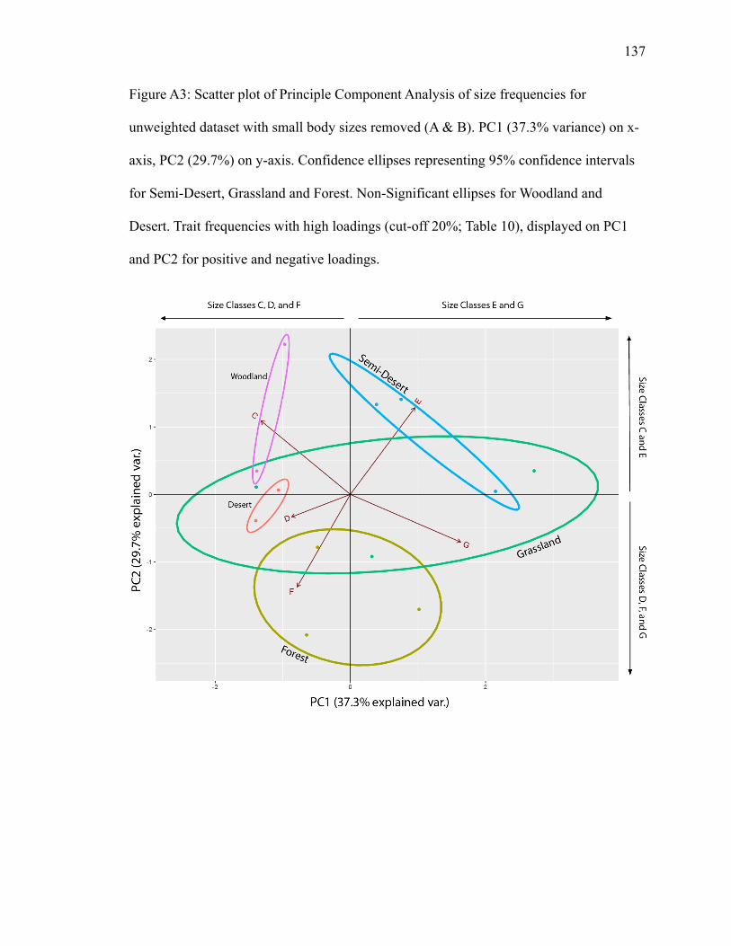
4.1.1.4 Unweighted Medium & Large Body Size PCA (≥ 500 g)

PC1 explains 37.3% of variance; PC2 explains 29.7% (Fig. A3). Grassland has

the largest ellipse and overlaps all biomes. Forest and semi-desert ellipses have clear

separation. Size class E plots in the semi-desert ellipse with high positive loadings on

both PC1 and PC2 (Table 10). Size class F plots in the forest ellipse in the opposite

direction with high negative loadings on PC1 and PC2 (Fig. A3; Table 10), suggesting an

inverse relationship between trait frequencies and their biomes. Size class D and G plot in

the grassland ellipse in opposite directions (Fig. A3), indicating a negative correlation

between the two size classes within the grassland biome. Size class D has high negative

loadings on PC1 and size class G has a high positive loading on PC1 and a high negative

loading on PC2 (Table 10).

21

4.1.2.1 Weighted Diet, Locomotion, Medium & Large Body Size (≥500 g) PCA

PC1 explains 28.4% of variance; PC2 explains 20.7% (Fig. 6). Semi-desert’s and

grassland’s ellipses have separation. Forest’s ellipse crosses both individually, creating

small pockets of overlap. Ambulatory and mixed feeder plot in the grassland ellipse.

Ambulatory and mixed feeder has a high negative loading on PC1. Aquatic/semi-aquatic

plots in the grassland ellipse in the opposite direction with low positive loadings on PC1

and PC2 (Fig. 6; Table 11), suggesting an inverse relationship. Arboreal/scansorial,

granivore, semi-fossorial, omnivore, and size class F plot in the forest ellipse.

Arboreal/scansorial, granivore, omnivore, and size class F have high positive loadings on

PC1 (Table 11). Arboreal/scansorial, granivore, and size class F have high negative

loadings on PC2 (Table 11). No trait classifications plot in the semi-desert ellipse, though

carnivore, non-cursorial and folivore trend towards semi-desert (Fig. 6).

4.1.2.2 Weighted Locomotion PCA, Medium & Large Body Size (≥500 g)

PC1 explains 30.2% of variance; PC2 explains 28.5% (Fig. 7). Grassland’s and

semi-desert’s ellipses show clear separation. Forest’s ellipse crosses into grassland

perpendicularly, creating an area of overlap. Arboreal/scansorial and semi-fossorial plot

together in the forest ellipse (Fig. 7), suggesting a positive relationship.

Arboreal/scansorial and semi-fossorial have high positive loadings on both PC1 and PC2

(Table 12). Cursorial and ambulatory plot in grassland, with aquatic/semi-aquatic plotting

in an opposite direction (Fig. 7), suggesting an inverse relationship among the three trait

frequencies. Cursorial and ambulatory have high positive loadings on PC1 and high

negative loadings on PC2 (Table 12). Fossorial plots in semi-desert with a high negative

loading on PC1 (Table 12).

22

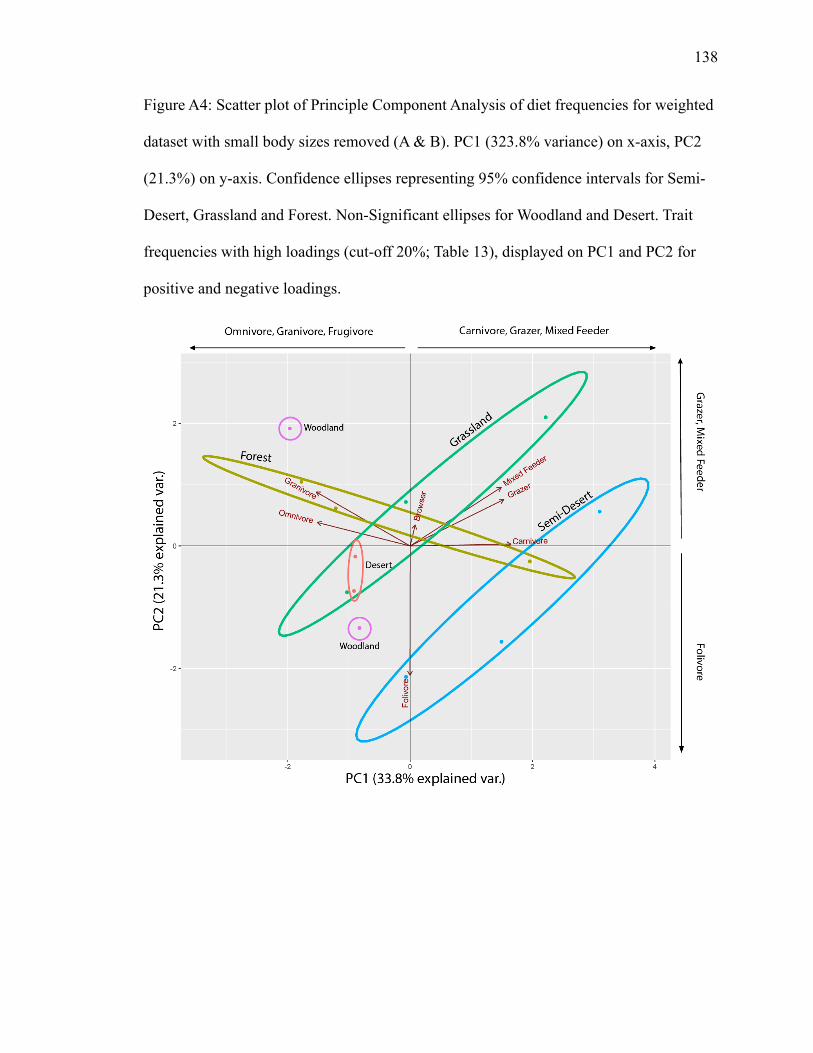
4.1.2.3 Weighted Diet PCA, Medium & Large Body Size (≥500 g)

PC1 explains 33.8% of variance; PC2 explains 21.3% (Fig. A4). Grassland’s and

semi-desert’s ellipses are separated, with the forest biome intersecting both

perpendicularly. Granivore plots in the forest ellipse with a high negative loading on PC1

and a high positive loading on PC2 (Table 13). Browser also plots in the forest ellipse,

though in area overlapping with grassland and with low loadings (Fig. A4; Table 13).

Folivore plots in semi-desert, with a high negative loading on PC2 (Table 13). No traits

plot inside grassland (Fig. A4).

4.1.2.4 Weighted Body Size PCA, Medium & Large Body Size (≥500 g)

PC1 explains 40.8% of variance; PC2 explains 31.7% (Fig. A5). Semi-desert has

the largest ellipse, overlapping forest’s ellipse. Grassland has the smallest ellipse,

crossing through forest’s and semi-desert’s ellipses perpendicularly. Size class F plots in

the forest ellipse (Fig. A5), with size classes D and E plotting in the opposite direction

(overlapped by semi-desert’s ellipse), suggesting a negative correlation. Size class F has a

high negative loading on PC2, size class D has a high positive loading on PC1 and a high

negative loading on PC2, and size class E has a high positive loading on PC1 (Table 14).

Size class G plots in the semi-desert ellipse, with a high positive loading on PC2 (Table

14).

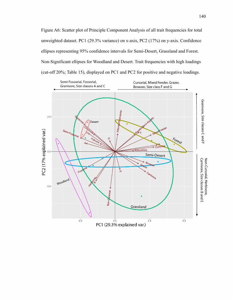
4.1.3.1 Total Unweighted PCA

PC1 explains 29.3% of variance; PC2 explains 17% (Fig. A6). Grassland displays

the largest ellipse, overlapping the other biomes. Semi-desert and forest have substantive

separation between their confidence ellipses. Aquatic/semi-aquatic, mixed feeder and size

class F plot in the forest ellipse. Mixed feeder and size class F have high positive

23

loadings on PC1 and size class F has a high positive loading on PC2 (Table 15).

Fossorial, grazer, and browser plot in the semi-desert ellipse. Browser and grazer plot

close together, with high positive loadings on PC1. Fossorial plots in the opposite

direction (Fig. A6) with a high negative loading on PC1, indicating a negative correlation

(Table 15). In the grassland ellipse, granivore, omnivore, folivore, semi-fossorial, and

size classes A and C group together (Fig. A6). From this first group, granivore and semi-

fossorial display high negative loadings on PC1, with granivore displaying a high

positive loading on PC2 (Table 15). Ambulatory, cursorial, and size class G plot together

in a separate direction (Fig. A6), suggesting an inverse relationship among the trait

frequencies. Cursorial and size class G have high positive loadings on PC1 (Table 15).

Herbivore, non-cursorial, and size class B also group separately in the grassland ellipse,

with all trait frequencies having high negative loadings on PC2 (Table 15).

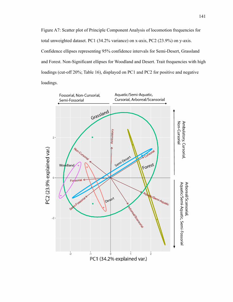
4.1.3.2 Total Unweighted Locomotion PCA


the largest ellipse and overlaps with other biomes. Forest and semi-desert cross

confidence ellipses, resulting in a small amount of separation. However, no trait

classifications plot inside either biome. Semi-fossorial and cursorial plot opposite of each

other close to forest’s ellipse (Fig. A7), suggesting a negative correlation, but do not plot

inside. Semi-fossorial has high negative loadings on PC1 and PC2, while cursorial has

high positive loadings on PC1 and PC2 (Table 16). Arboreal/scansorial and non-cursorial

plot in the grassland ellipse, with no overlap and in opposite directions (Fig. A7),

indicating an inverse relationship. Arboreal/scansorial has a high positive loading on PC1

and a high negative loading on PC2, while non-cursorial has a high negative loading on

24

PC1 and a high positive loading on PC2 (Table 16). Fossorial, ambulatory, and

aquatic/semi-aquatic additionally plot in opposite directions (Fig. A7), with aquatic/semi-

aquatic plotting close to the semi-desert ellipse. Fossorial has a high negative loading and

aquatic/semi-aquatic has a high positive loading on PC1. Ambulatory has a high positive

loading on PC2 with a high negative loading from aquatic/semi-aquatic (Table 16).

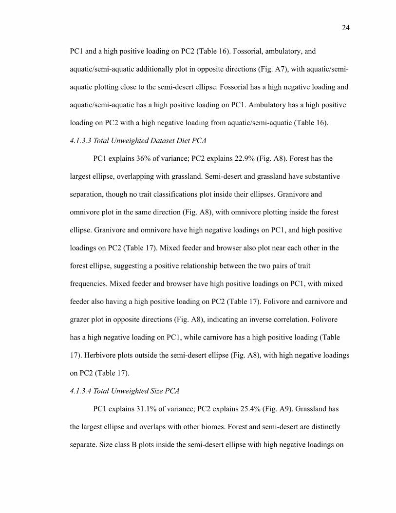
4.1.3.3 Total Unweighted Dataset Diet PCA

PC1 explains 36% of variance; PC2 explains 22.9% (Fig. A8). Forest has the

largest ellipse, overlapping with grassland. Semi-desert and grassland have substantive

separation, though no trait classifications plot inside their ellipses. Granivore and

omnivore plot in the same direction (Fig. A8), with omnivore plotting inside the forest

ellipse. Granivore and omnivore have high negative loadings on PC1, and high positive

loadings on PC2 (Table 17). Mixed feeder and browser also plot near each other in the

forest ellipse, suggesting a positive relationship between the two pairs of trait

frequencies. Mixed feeder and browser have high positive loadings on PC1, with mixed

feeder also having a high positive loading on PC2 (Table 17). Folivore and carnivore and

grazer plot in opposite directions (Fig. A8), indicating an inverse correlation. Folivore

has a high negative loading on PC1, while carnivore has a high positive loading (Table

17). Herbivore plots outside the semi-desert ellipse (Fig. A8), with high negative loadings

on PC2 (Table 17).

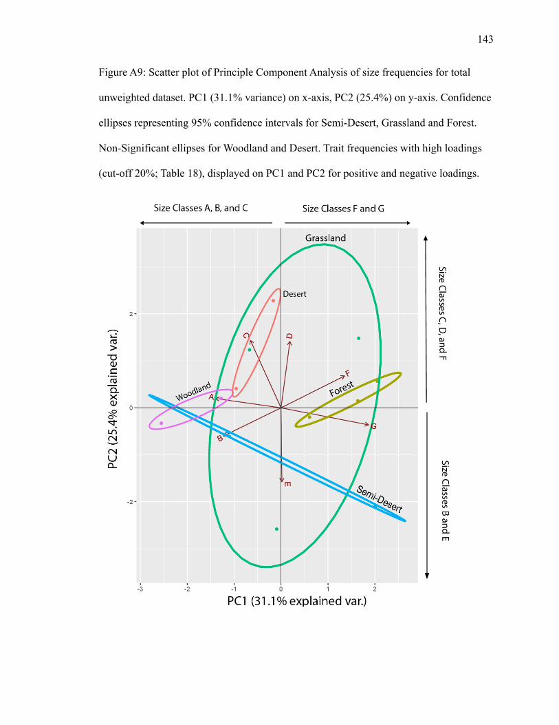
4.1.3.4 Total Unweighted Size PCA


the largest ellipse and overlaps with other biomes. Forest and semi-desert are distinctly

separate. Size class B plots inside the semi-desert ellipse with high negative loadings on

25

PC1 and PC2 (Table 18). Size classes A, C, and D plot in grassland. Size classes A and C

have high negative loadings on PC1, and size classes C and D have high positive loadings

on PC2 (Table 18). Size classes E and G also plot in the grassland ellipse. Size class G

has a high positive loading on PC1 and size class E a high positive loading on PC2 (Table

18). Size class A plots opposite of G, and size class D opposite of E (Fig. A9), suggesting

negative correlations.

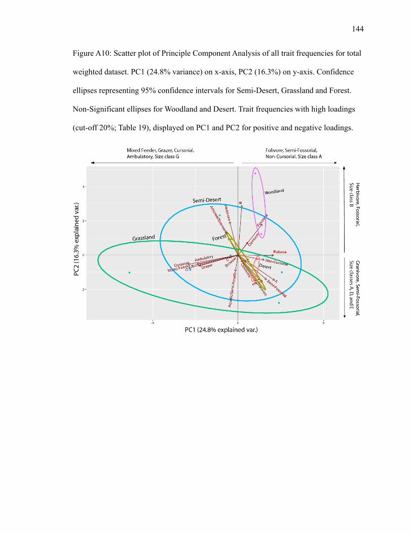
4.1.4.1 Total Weighted PCA

PC1 explains 24.8%; PC2 explains 16.3% (Fig. A10). Grassland has the largest

ellipse, overlapping with forest and semi-desert ellipses. Semi-desert has the second

largest ellipse and overlaps the forest ellipse. Herbivore, fossorial, folivore, and carnivore

plot in the semi-desert ellipse. Folivore has a high positive loading on PC1, while

herbivore, and fossorial have high positive loadings on PC2 (Table 19).

Arboreal/scansorial plots in the forest ellipse, along with size classes D and F in the

opposite direction (Fig. A10), suggesting a negative correlation. Size class D has a high

negative loading on PC2 (Table 19). Browser plots just outside of the forest ellipse,

landing in the middle of the groups and has substantially low loadings on PC1 and PC2

(Table 19). Cursorial, mixed feeder, ambulatory, grazer, and size classes G and C all plot

in the grassland and semi-desert ellipses. Cursorial, mixed feeder, ambulatory, grazer,

and size class G have high negative loadings on PC1 (Table 19). Non-cursorial, semi-

fossorial, granivore, omnivore, and size classes A and E plot in the grassland and semi-

desert ellipses in the opposite direction (Fig. A10), indicating an inverse relationship

between the two groups. Non-cursorial, semi-fossorial, and size class A have high

positive loadings on PC1. Size class A, semi-fossorial, and granivore have high negative

26

loadings on PC2 (Table 19). Aquatic/semi-aquatic plots in the grassland and semi-desert

ellipses, landing between those groups (Fig. A10).

4.1.4.2 Total Weighted Locomotion PCA

PC1 explains 32.8%; PC2 explains 21.1% (Fig. A11). Grassland, forest, and semi-

desert have close to equal sized ellipses, and all overlap in some areas. Forest’s ellipse

overlaps with semi-desert’s ellipse and a small amount of grassland’s. Fossorial and

aquatic/semi-aquatic plot in the semi-desert ellipse in regions with no overlap and plot in

opposite directions (Fig. A11), suggesting an inverse relationship. Fossorial has a high

negative loading on PC1 (Table 20). Ambulatory and cursorial plot in the grassland

ellipse, with ambulatory and cursorial having high positive loadings on PC1 and PC2

(Table 20). Semi-fossorial and non-cursorial plot in the grassland and semi-desert

ellipses. Semi-fossorial and non-cursorial have high negative loadings on PC1 and high

positive loadings on PC2 (Table 20). Arboreal/scansorial plots in the forest and semi-

desert ellipses, in the opposite direction of semi-fossorial and non-cursorial (Fig. A11),

suggesting a negative correlation. Arboreal/scansorial has a high positive loading on PC1

and a high negative loading on PC2 (Table 20).

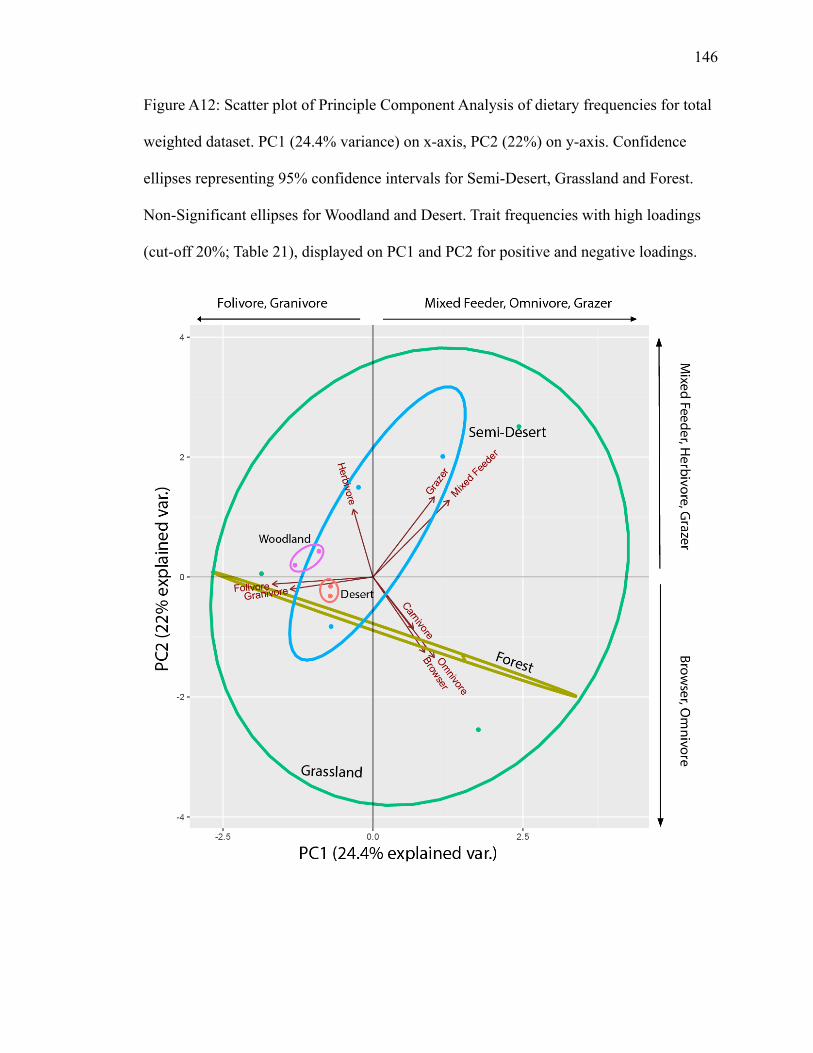
4.1.4.3 Total Weighted Diet PCA

PC1 explains 24.4% of variance; PC2 explains 22% (Fig. A12). Grassland has the

largest ellipse, encompassing all biomes. Semi-desert’s ellipse overlaps with forest’s.

Mixed feeder and grazer plot close together, with grazer landing in the semi-desert and

grassland ellipses and mixed feeder just in the grassland ellipse (Fig. A12). Mixed feeder

and grazer have high positive loadings on PC1 and PC2 (Table 21). Herbivore also plots

in the semi-desert and grassland ellipses, with herbivore having a high positive loading

27

on PC2 (Table 21). Folivore and granivore plot close to each other in the grassland ellipse

and in the opposite direction of carnivore, omnivore, and browser (Fig. A12), suggesting

a negative relationship between the sets of trait frequencies and a positive relationship

within the two sets. Folivore and granivore have high negative loadings on PC1 (Table

21). Carnivore, omnivore and browser have high positive loadings on PC1 and high

negative loadings on PC2 (Table 21).

4.1.4.4 Total Weighted Size PCA

PC1 explains 34.1% of variance; PC2 explains 22.5% (Fig. A13). Forest and

semi-grassland form circular confidence intervals, while grassland forms an elliptical

interval. There is a high level of overlap among all the biome ellipses. Size class A and B

plot in the forest ellipse (without overlap) and in different directions (Fig. A13),

suggesting an inverse relationship. Size class A has a high positive loading and size class

B has a high negative on PC1, while both size classes have high negative loadings on

PC2 (Table 22). Size classes D and E plot close to each other (Fig. A13), indicating a

positive correlation. Size class D plots inside all three biomes, with a high positive

loading on PC1, and size class E plots in the semi-desert and forest ellipses with high

positive loadings on PC1 and PC2 (Table 22). Size classes C and G also plot close and

inside all three biomes (Fig. A13), suggesting a positive relationship. Size class C has a

high positive loading on PC2 (Table 22). Size class F plots in the semi-desert and forest

ellipses, with low loadings on PC1 and PC2 (Table 22).

4.1.5.1 Rodents and Lagomorphs Unweighted PCA

PC1 explains 27.4% of variance; PC2 explains 22.3% (Fig. A14). Grassland,

forest, and semi-desert all have similar sizes of ellipses and overlap each other. Folivore,

28

aquatic/semi-aquatic, and size class F and G plot within the forest ellipse. Semi-fossorial

and omnivore plot in the grassland ellipse in opposite directions (Fig. A14), suggesting a

negative relationship. Semi-fossorial has a high positive loading on PC2 (Table 23). Non-

cursorial and size class D plot in the semi-desert ellipse. Non-cursorial has a high positive

loading on PC1 and high negative loading on PC2 (Table 23). Carnivore plots in the

grassland and semi-desert ellipses and plots opposite of non-cursorial (Fig. A14),

indicating an inverse correlation.

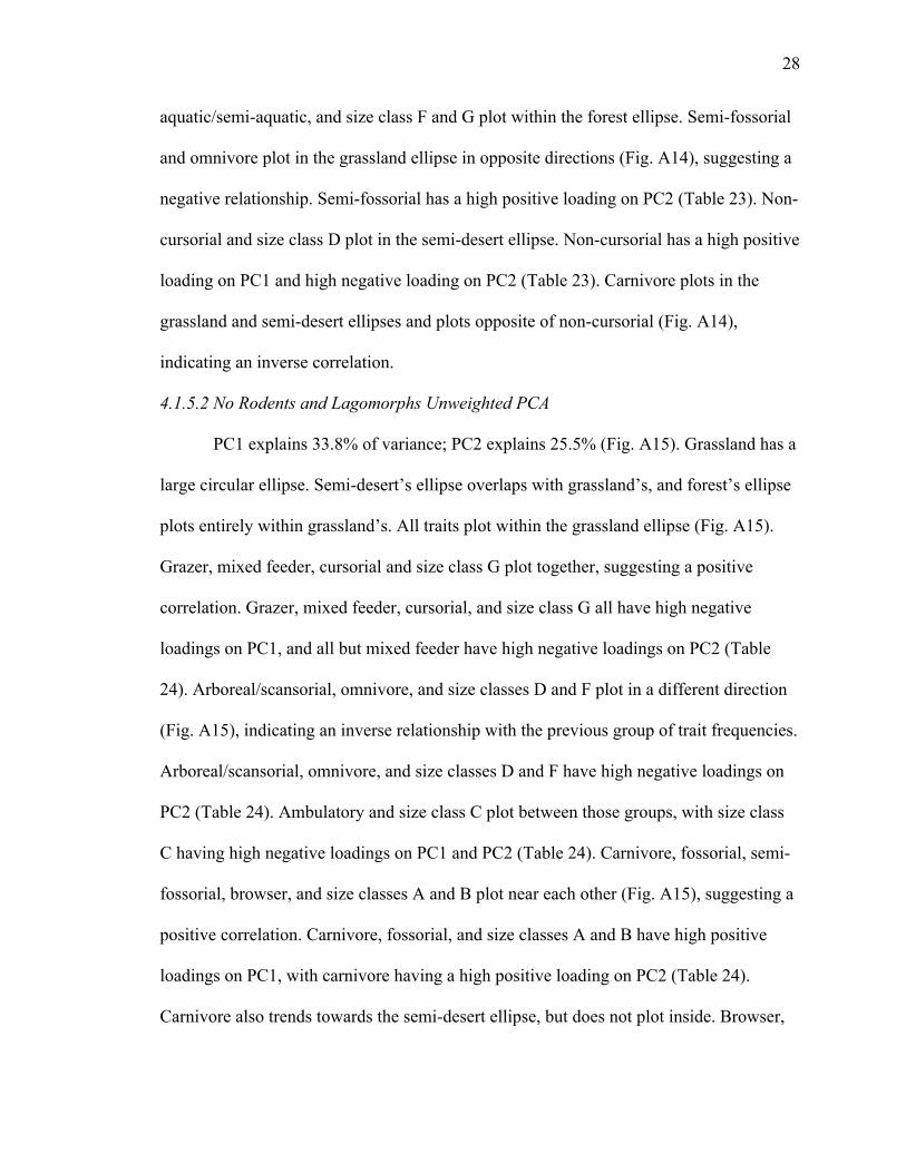
4.1.5.2 No Rodents and Lagomorphs Unweighted PCA

PC1 explains 33.8% of variance; PC2 explains 25.5% (Fig. A15). Grassland has a

large circular ellipse. Semi-desert’s ellipse overlaps with grassland’s, and forest’s ellipse

plots entirely within grassland’s. All traits plot within the grassland ellipse (Fig. A15).

Grazer, mixed feeder, cursorial and size class G plot together, suggesting a positive

correlation. Grazer, mixed feeder, cursorial, and size class G all have high negative

loadings on PC1, and all but mixed feeder have high negative loadings on PC2 (Table

24). Arboreal/scansorial, omnivore, and size classes D and F plot in a different direction

(Fig. A15), indicating an inverse relationship with the previous group of trait frequencies.

Arboreal/scansorial, omnivore, and size classes D and F have high negative loadings on

PC2 (Table 24). Ambulatory and size class C plot between those groups, with size class

C having high negative loadings on PC1 and PC2 (Table 24). Carnivore, fossorial, semi-

fossorial, browser, and size classes A and B plot near each other (Fig. A15), suggesting a

positive correlation. Carnivore, fossorial, and size classes A and B have high positive

loadings on PC1, with carnivore having a high positive loading on PC2 (Table 24).

Carnivore also trends towards the semi-desert ellipse, but does not plot inside. Browser,

29

non-cursorial, and semi-fossorial plot past forest’s ellipse, but do not plot inside its region

(Fig. A15).

4.2 Trait Composition – Stacked Area Charts

Stacked area charts consist of biomes on the x-axis, ordered from closed to open

(left to right) and percentage on the y-axis, marked every 20%. Composition of trait

frequencies for locomotion, diet, and body mass are displayed for each biome. Changes

or trends in trait composition can be observed within biomes vertically or across biomes

horizontally.

4.2.1a Total Unweighted Locomotion

Ambulatory and aquatic/semi-aquatic trait percentages make up a minimal

amount of the total community in all biomes, not appearing at all in woodland (Fig. 8;

Table 5-A). Out of the two, aquatic/semi-aquatic occurs with higher frequency in forest

(3.9%) and ambulatory with frequency higher in grassland (2.08%). They are equal in

desert (1.6%), and ambulatory doesn't appear in semi-desert. There is an increase of semi-

fossorial and fossorial traits from forest (18.6%; 20.5%) to desert (29.5%; 26.2%), with a

sharper increase in woodland (31.9%; 29.7%). Arboreal/scansorial is highest in forest

(28.4%) and drops slightly from forest to desert (19.6%). Cursorial is smallest in

woodland (6.3%) and increases in the more open biomes. Non-cursorial is smallest in

forest (9.8%) and desert (8.2%), increasing in semi-desert (16.8%).

4.2.1b Total Unweighted Diet

Browser makes up very little of the composition in forest (1.9%) and grassland

(1.04%) (Fig. 8; Table 5-B). Grazer only appears in grassland (2.08%) and semi-desert

(2.6%), making up a low percentage. Granivore stays constant across the biomes. Mixed

30

feeder and herbivore do as well; however, herbivore increases (10.6%) and mixed feeder

drops out in woodland. Carnivore has a significant amount in forest (31.3%), dropping

steadily across the biomes to desert (13.1%). Folivore has a high amount in semi-desert

(36.3%) but stays constant in the other biomes. Omnivore stays constant as well,

decreasing in semi-desert (10.3%).

4.2.1c Total Unweighted Size

Size classes A (0-50 g) and B (50-500 g) make up half of the total composition in

every biome, reaching about 60% in woodland. Size classes C (500-1000 g), D (1000 –

1500 g), E (1500 – 3500 g), and F (3500 – 10500 g) are relatively equal (Fig. 8; Table 5-

C). Size class E is slightly higher (12.9%), and size class C (10.3%) is slightly lower in

semi-desert. Size class C also has a slight increase from forest (7.8%) to desert (16.3%).

Size class F slightly drops from forest (13.7%) to desert (8.2%), dropping more in semi-

desert (2.6%). Size class G (>10500 g) lowers in woodland (4.2%) while increasing in

grassland (19.7%) and semi-desert (20.7%).

4.2.2a Medium & Large Mammals (≥500 g), Unweighted Locomotion

Aquatic/semi-aquatic and ambulatory, while still low, have a higher presence in

the composition of biomes, dropping out in woodland and semi-desert (for ambulatory).

Ambulatory appears more in grassland (3.8%), while aquatic/semi-aquatic appears more

in forest (5.7%) (Fig. 9; Table 6-A). They occur equally in desert (3.4%). Semi-fossorial

is low in all biomes but does have a slight decrease from forest (5.7%) to desert (3.4%).

Arboreal/scansorial and cursorial make up more than half of forest (32.6%; 34.6%), then

decrease in woodland (21.4%). There is no clear pattern across biomes for either of

arboreal/scansorial or cursorial. Cursorial increases more in grassland (34.6%) and

31

remains constant. Arboreal/scansorial decreases in semi-desert (5%) but increases again

in desert (24.1%). Fossorial increases from forest (9.6%) to desert (20.6%), with a

substantial increase in woodland (28.5%). Non-cursorial also increases from forest

(9.6%) to desert (17.2%). Semi-fossorial remains low from forest (5.7%) to desert

(3.4%).

4.2.2b Medium & Large Mammals (≥500 g), Unweighted Diet

Browser appears in only forest (3.8%) and grassland (1.9%) and makes up a small

amount of the composition (Fig. 9; Table 6-B). Grazer appears in grassland (3.8%) and

semi-desert (5%) but does not make up a significant proportion of the composition.

Mixed feeder drops out of woodland, with a slight decrease from forest (11.5%) to desert

(3.4%). Granivore decreases slightly from forest (15.3%) to desert (13.7%), dropping

significantly in semi-desert (2.5%). Carnivore remains roughly the same, decreasing

slightly in woodland (14.2%) and desert (17.2%), and increasing again in grassland

(23.08%) and semi-desert (27.5%). Folivore makes up a significant proportion of every

biome, and peaks above half in semi-desert (55%). Omnivore increases slightly from

forest (19.2%) to desert (27.5%), with a more substantial increase in woodland (28.5%)

and a substantial decrease in semi-desert (2.5%).

4.2.2c Medium & Large Mammals (≥500 g), Unweighted Size

With size classes A and B (<500 g) removed, it is easier to see the proportions of

the remaining size classes (Fig. 9; Table 6-C). Size classes C (500 – 1000 g) and G

(>10500 g) make up around half of the composition in all biomes. Size class C increases

in woodland (42.8%) and desert (34.4%), but decreases in forest (15.3%) and semi-desert

(20%). Size class G increases in forest (34.6%), grassland (36.5%), and semi-desert

32

(40%). Size class D (1000 – 1500 g) remains the same across the biomes. Size class E

(1500 – 3500 g) increases in woodland (21.4%) and semi-desert (25%). Size class F

(3500 – 10500 g) decreases from forest (26.9%) to desert (17.2%), notably decreasing in

semi-desert (5%).

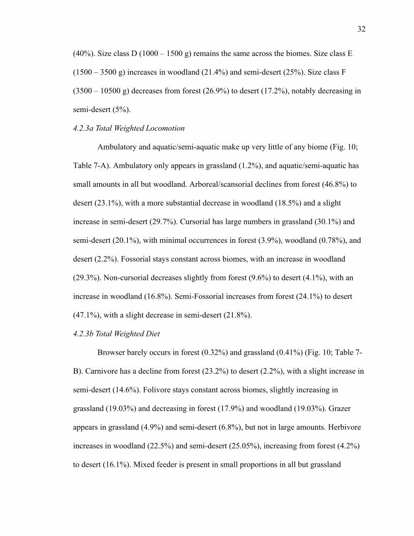
4.2.3a Total Weighted Locomotion

Ambulatory and aquatic/semi-aquatic make up very little of any biome (Fig. 10;

Table 7-A). Ambulatory only appears in grassland (1.2%), and aquatic/semi-aquatic has

small amounts in all but woodland. Arboreal/scansorial declines from forest (46.8%) to

desert (23.1%), with a more substantial decrease in woodland (18.5%) and a slight

increase in semi-desert (29.7%). Cursorial has large numbers in grassland (30.1%) and

semi-desert (20.1%), with minimal occurrences in forest (3.9%), woodland (0.78%), and

desert (2.2%). Fossorial stays constant across biomes, with an increase in woodland

(29.3%). Non-cursorial decreases slightly from forest (9.6%) to desert (4.1%), with an

increase in woodland (16.8%). Semi-Fossorial increases from forest (24.1%) to desert

(47.1%), with a slight decrease in semi-desert (21.8%).

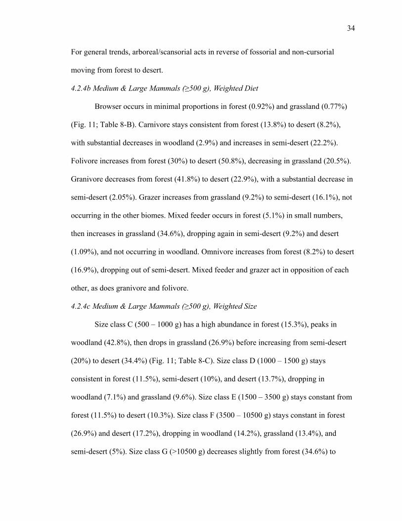
4.2.3b Total Weighted Diet

Browser barely occurs in forest (0.32%) and grassland (0.41%) (Fig. 10; Table 7-

B). Carnivore has a decline from forest (23.2%) to desert (2.2%), with a slight increase in

semi-desert (14.6%). Folivore stays constant across biomes, slightly increasing in

grassland (19.03%) and decreasing in forest (17.9%) and woodland (19.03%). Grazer

appears in grassland (4.9%) and semi-desert (6.8%), but not in large amounts. Herbivore

increases in woodland (22.5%) and semi-desert (25.05%), increasing from forest (4.2%)

to desert (16.1%). Mixed feeder is present in small proportions in all but grassland

33

(18.4%) and doesn't appear in woodland or desert. Omnivore is highest in forest (33.5%)

and desert (29.98%) and decreases from woodland (18.5%) to semi-desert (15.1%).

4.2.3c Total Weighted Size

Size classes A (0 – 50 g) and B (50 – 500 g) make up more than half up the

composition in any biome, with size class B higher than size class A (Fig. 10; Table 7-C).

Size class A does increase from forest (17.2%) to desert (39.5%), with a slight dip in

semi-desert (13.8%). Size class B increases from forest (47.7%) to woodland (67.1%),

drops in grassland (26.5%), then increases again in semi-desert (43.7%) and desert

(40.5%). Size class C (500 – 1000 g) stays constant across biomes, decreasing very

slightly in woodland (9.3%) and desert (8.4%). Size classes D (1000 – 1500 g), E (1500 –

3500 g), and F (3500 – 10500 g) stay constant, as well, but make up a much smaller part

of the composition. Size class G (>10500 g) is small except in grassland (31.7%) and

semi-desert (19.6%).

4.2.4a Medium & Large Mammals (≥500 g), Weighted Locomotion

Ambulatory appears in grassland (0.13%) in minimal proportions (Fig. 11; Table

8-A). Aquatic/semi-aquatic increases from forest (0.92%) to desert (11.4%), dropping out

of woodland and decreasing in semi-desert (0.51%). Arboreal/scansorial decreases from

forest (58.5%) to desert (33.3%), significantly decreasing in semi-desert (2.3%) and

increasing slightly in desert. Cursorial stays consistent from forest (11.3%) to desert

(11.4%), with large increases in grassland (56.6%) and semi-desert (47.5%). Fossorial

increases across biomes, decreasing slightly in grassland (9.6%). Non-cursorial increases

from forest (15.3%) to desert (20.7%), with a dip in grassland (9.7%). Semi-fossorial

decreases from forest (8.2%) to woodland (3.8%), barely occurring in grassland to desert.

34

For general trends, arboreal/scansorial acts in reverse of fossorial and non-cursorial

moving from forest to desert.

4.2.4b Medium & Large Mammals (≥500 g), Weighted Diet

Browser occurs in minimal proportions in forest (0.92%) and grassland (0.77%)

(Fig. 11; Table 8-B). Carnivore stays consistent from forest (13.8%) to desert (8.2%),

with substantial decreases in woodland (2.9%) and increases in semi-desert (22.2%).

Folivore increases from forest (30%) to desert (50.8%), decreasing in grassland (20.5%).

Granivore decreases from forest (41.8%) to desert (22.9%), with a substantial decrease in

semi-desert (2.05%). Grazer increases from grassland (9.2%) to semi-desert (16.1%), not

occurring in the other biomes. Mixed feeder occurs in forest (5.1%) in small numbers,

then increases in grassland (34.6%), dropping again in semi-desert (9.2%) and desert

(1.09%), and not occurring in woodland. Omnivore increases from forest (8.2%) to desert

(16.9%), dropping out of semi-desert. Mixed feeder and grazer act in opposition of each

other, as does granivore and folivore.

4.2.4c Medium & Large Mammals (≥500 g), Weighted Size

Size class C (500 – 1000 g) has a high abundance in forest (15.3%), peaks in

woodland (42.8%), then drops in grassland (26.9%) before increasing from semi-desert

(20%) to desert (34.4%) (Fig. 11; Table 8-C). Size class D (1000 – 1500 g) stays

consistent in forest (11.5%), semi-desert (10%), and desert (13.7%), dropping in

woodland (7.1%) and grassland (9.6%). Size class E (1500 – 3500 g) stays constant from

forest (11.5%) to desert (10.3%). Size class F (3500 – 10500 g) stays constant in forest

(26.9%) and desert (17.2%), dropping in woodland (14.2%), grassland (13.4%), and

semi-desert (5%). Size class G (>10500 g) decreases slightly from forest (34.6%) to

35

desert (24.1%), increasing substantially in grassland (36.5%) before decreasing slightly

from semi-desert (40%) to desert. Size class C and G have an opposing relationship,

whereas the other size classes remain constant among the biomes.

36

5. DISCUSSION

5.1 PCA Analyses

Unweighted datasets generally exhibit the highest degree of separation among

biomes. The dataset with traits from all three categories (diet, locomotion, and body

mass) for medium and large mammals (≥ 500g), showed especially clear separation

among grassland, forest, and semi-desert (Fig. 3). Notably, in this dataset a clear gradient

from forest to grassland to semi-desert is captured. This pattern is similar to patterns

expected across a precipitation gradient. Differences in precipitation across the biomes

are observed when recorded climate data for the biome ecocodes are compiled and annual

averages are calculated (Table A5; Bailey 1995). In Figure 3, vertical separation is

observed between semi-desert, grassland, and forest, representing differences present on

PC2. This vertical succession matches with annual average precipitation differences for

the three biomes (Table A5). Semi-desert has an annual precipitation average of 412.75

mm, grassland 706.12 mm, and forest 1100.6 mm. Semi-desert plots completely in the

positive side of PC2, forest plots completely on the negative, and grassland plots in both

positive and negative (Fig. 3). The positive end of the second principle component’s axis

appears to match with lower annual precipitation averages, and the negative end matches

with higher precipitation averages. This gradient suggests that PC2 represents

precipitation for this primary analysis.

In the unweighted PCA of all traits (Fig. 3), the grassland biome has the broadest

range of traits. Grazer, cursorial, aquatic/semi-aquatic, and size class G (>10,500 g) plot

in the western quadrant of the biome, while size classes C (500 – 1,000 g) and D (1,000 –

1,500 g) plot on the opposite end. Grazer, cursorial, and size class G are closely

37

correlated with each other. Additionally, they have high associations with the first

principle component. This suggests that grazer, cursorial, and size class G are the key

traits for defining grassland. Cursorial and size class G have similar occurrence

frequencies in the overall trait composition, as well, composing about a third of

grassland’s trait composition. Grazer occurs in much lower frequencies, but still is an

important trait within grassland (Fig. 9). The forest biome contains fewer traits that are all

clustered in the west and northwest quadrant of the biome, plotting in the southeast

quadrant of the entire PCA. Granivore, omnivore, and arboreal/scansorial plot together in

the forest ellipse and appear to have a close correlation with each other. They also have

high positive loadings on the first principle component, as opposed to the strongly

negative loadings from grazer, cursorial, and size class G (Table 7), suggesting an inverse

correlation between the two sets of trait frequencies. Granivore, omnivore, and

arboreal/scansorial all also have high negative loadings on the second principle

component, suggesting these three trait frequencies are more associated with higher

levels of precipitation. Size class F, while not clustering with the other trait frequencies in

the forest ellipse, also has a high negative loading on PC2, suggesting mammals with

body masses of 3,500 g to 10,500 g prefer biomes with higher annual precipitation. It is

unlikely, however, that precipitation has a direct effect on body mass. Rather, body mass

is probably correlated with the “openness” of the biome, with lower rainfall in more open

areas (grasslands) and higher rainfall in more closed areas (forests).

In the unweighted analysis of all traits (Fig. 3), arboreal/scansorial comprises

about 30% of total trait composition for forest (Fig. 9). Omnivore and granivore

individually occur with lower frequency but together comprise about 40% of total trait

38

composition (Fig. 9). However, these trait frequencies (cursorial, granivore, omnivore,

arboreal/scansorial, size class G) are rather consistent among biomes (Fig. 9; Table 2),

potentially due to sampling and collection bias. Both subsamples of woodland plot inside

the forest ellipse, in the western quadrant, and plot closest to size class C (500–1,000 g).

Although it might be expected that woodland would plot between forest and grassland,

because it contains a mixture of both, in this analysis the forest component appears to be

stronger. One subsample of desert plots inside forest, in the southwestern quadrant, near

size class D (1,000–1,500 g). The second subsample of desert plots outside any biome’s

ellipse and does not align with any traits (Fig. 3).

Separation among the forest, grassland, and semi-desert biomes is visible when

the locomotion is analyzed separately, with forest and semi-desert separated by grassland

(Fig. 4). This is similar to the gradient visible with all trait frequencies analyzed together

(Fig. 3); however, the biomes have flipped on the second principle component axis. In the

locomotion analysis, semi-desert plots entirely on the negative side on PC2, forest plots

entirely in the positive, and grassland remains between these two (Fig. 4). Again, a

precipitation gradient is suggested, only with the gradient flipped. The negative side of

the second principle component axis matches with lower annual precipitation averages,

while the positive side matches with higher averages. In the locomotion analysis, non-

cursorial has a positive correlation with the semi-desert biome (Fig. 4). Non-cursorial has

an especially high negative loading on PC2 (Table 8), indicating its association with low

levels of precipitation. Non-cursorial taxa (i.e., Lepus townsendii, Lepus californicus,

Sylvilagus nuttalli) make up just under a quarter of locomotion composition in the semi-

desert biome (Fig. 9), suggesting it is an important trait for distinguishing semi-desert.

39

Cursorial has a positive correlation with the grassland biome (Fig. 4) and a high negative

loading on the second principle component (Table 8). Cursorial appears to also have an

association with open environments. Cursorial plots in the grassland ellipse on the

negative side of the second principle component (Fig. 4), suggesting its association with

the drier areas of the grassland biome. Cursorial also occurs with a high proportion in

grassland (Fig. 9). Arboreal/scansorial has a positive correlation with the forest biome

and a high positive loading on PC2 (Table 8). Arboreal/scansorial appears to have a high

association with closed environments. As mentioned above, arboreal/scansorial

comprises about 30% of the trait composition for the forest biome (Fig. 9), coming in

second for frequency. Due to its high correlation (Fig. 4), arboreal/scansorial is clearly an

important trait for distinguishing the forest biome, as would be expected. The locomotion

analysis appears to identify locomotion frequencies that accurately distinguish biomes,

providing a higher resolution analysis compared to all the traits combined.

Separation among the forest, grassland, and semi-desert biomes is also achieved

when diet is analyzed separately, with forest and semi-desert separated by grassland (Fig.

5), as in the previous analyses (Fig. 3 & 4). The diet analysis follows the same

precipitation gradient as locomotion, with lower annual averages matching with the

negative side of the second principle component axis and higher annual averages with the

positive. Semi-desert plots mainly in the negative side of PC2, while forest plots mainly

in the positive side (Fig. 5). Grazer still has a high positive loading on PC2 (Table 9),

suggesting its association with closed environments. Mixed feeder plots within the

grassland ellipse, with a high positive loading on PC2. Mixed feeder plots in grassland on

the positive side of the second principle component axis (Fig. 5), indicating its

40

association with the wetter areas of the biome. Within forest, granivore and omnivore

maintain their correlation with each other when diet is analyzed separately (Fig. 5).

Omnivore has a high positive loading on PC2, suggesting an association with closed

environments. Browser also has high positive loadings on PC2 (Table 9). Browser also

plots in the more positive end of forest on the second principle component axis, while

omnivore and granivore plot closer to the negative side of the axis. Browser appears to

also be associated with closed environments in the forest biome.

Unlike the other traits, body mass does not clearly distinguish biomes when

analyzed separately (Fig. A3). The forest and semi-desert biomes are overlapped by the

grassland biome, contrary to the expected gradient (Fig. 3, 4, & 5). Size class E (1,500 –

3,500 g) has a positive correlation with the semi-desert biome (Fig. A3). Size class E

composes a fourth of the trait composition in the semi-desert biome; however, size class

G (>10,500 g) dominates the composition (Fig. 9). Size class E is important for

distinguishing the semi-desert biome, regardless of its low occurrence. Size classes D

(1,000 – 1,500 g) and G (>10,500 g) have an inverse relationship in the grassland biome,

plotting on opposite ends of the ellipse and with opposite loadings (Fig. A5; Table 10).

Body mass does not do an effective job separating the biomes when analyzed separately,

yet certain body mass frequencies have positive correlations with diet and locomotion

when all traits are analyzed.

Significant biases may exist in the datasets due to a low number of ungulates (see

discussion below). As a possible compensation, datasets were weighted by the number of

occurrences of individual taxa within a biome before PCA analysis. This method may

help compensate for situations where a trait occurs in a few taxa, but these taxa are

41

abundantly represented and geographically widespread. An example is Bison bison,

which was historically widespread and abundant. Grasslands favored by B. bison may

have supported a low diversity of grazing ungulates but the abundance of B. bison

compensated for this low diversity with a significant biomass of grazing individuals.

However, although this method could hypothetically help compensate for low species

diversity, the weighted PCAs done here do not appear to separate biomes as well as the

more conventional unweighted analyses.

Weighted data with no small body sizes (<500 g) show separation between the

semi-desert and grassland biomes (Fig. 6), following the gradient displayed in the

unweighted data (Fig. 3). The forest biome crosses perpendicularly both the semi-desert

and grassland biomes (Fig. 6); however, many of the trait frequencies plotted in forest are

in the negative side of the ellipse, where there is no overlap. The precipitation gradient

observed in Figure 3 roughly applies here, with lower annual precipitation averages

matching with the positive side of the second principle component axis, and higher

annual averages with the negative side. Trait frequencies are more tightly clustered,

forming three distinct sets of correlations (Fig. 6): grazer, cursorial, mixed feeder,

carnivore, ambulatory, and size class G; non-cursorial, folivore, fossorial, and size classes

D and E; and omnivore, arboreal/scansorial, granivore, semi-fossorial, and size classes C

and F. Granivore, omnivore, semi-fossorial, arboreal/scansorial, and size classes C and F

plot close to each other in forest, having a positive strong correlation (Table 11).

Granivore, arboreal/scansorial, semi-fossorial, and size class F also have high negative

loadings on PC2, suggesting an association with more closed environments.

Arboreal/scansorial occurs with over half of the occurrence in forest, followed by

42

granivore just under half (Fig. 11; Table 6A & 6B). Browser does plot in forest; however,

browser shows low correlation with other trait frequencies (Table 11) and plots where

there is overlap with grassland (Fig. 6). Alces alces is the only taxon classified as a

browser, but it occurs equally in the grassland and forest biomes with seven occurrences.

Non-cursorial, folivore, fossorial, and size classes D and E have a positive correlation

with each other, all with high positive loadings on PC2, indicating an association with

open environments. Mixed feeder, grazer, cursorial, carnivore, ambulatory and size class

G have a positive correlation with each other in the grassland biome (Table 11).

Ambulatory only occurs in one taxon (Ursus americanus), but has a large number of

occurrences in grassland. Mixed feeder occurs in many of the ungulate taxa (Antilocapra

americana, Odocoileus hemionus, Odocoileus virginianus, Cervus canadensis, Rangifer

tarandus). Antilocapra americana and Odocoileus hemionus occur in very high numbers

in grassland. Both ambulatory and mixed feeder represent another trait occurring in a low

number of taxa that are abundantly represented.

Both the unweighted and weighted datasets with the full range of body sizes

included show poor separation of biomes when the total data are analyzed together. The

total unweighted dataset does show separation between the semi-desert and forest

biomes. However, grassland overlaps both, and all trait frequencies plot in the grassland

biome and show no distinction for other biomes (Fig. A6). The total weighted dataset

shows no separation among the forest, grassland, and semi-desert biomes (Fig. A10).

There are a few trait frequencies that plot in an area of the semi-desert biome not

overlapped by the grassland or forest ellipses, but no clear correlation among trait

frequencies is observed (Fig. A10). Associations with closed or open environments are

43

not evident in either analysis. Lack of significant separation of biomes indicate small-

bodied mammals are masking correlations that are seen without these mammals.

Comparing the total unweighted dataset with the unweighted dataset with small-bodied

mammals removed, relationships among trait frequencies are clear and correspond to

biome separation with small-bodied mammals removed (Fig. 3). With the total dataset,

correlations among trait frequencies are less clear and do not relate to biomes, as there is

substantial overlap and no significant separation (Fig. A6). Additionally, mammals

smaller than 500 g make up 51% of the total unweighted dataset, and in the weighted

dataset, that proportion jumps to 64.5%. Visible in Figures 8 & 9, the relationships of the

size frequencies in the unweighted dataset are better observed with the small-bodied

mammals removed.

5.2 Sources of Potential Biases

In considering the high amount of overlap by grassland in almost all analyses of

total data (e.g., Fig. A6, A7, A9, A10, A12), it is important to note that trait data were not

collected directly from the taxa being sampled. Instead, I gathered trait data from the

literature and from databases. For some specialist taxa (e.g., bison, wolves, moles) traits

are not going to differ among biomes. However, generalist taxa may not match their

recorded trait classification with behavior in certain biomes. For example, many squirrels

are classified as arboreal/scansorial but also occur in grasslands. This clearly does not

reflect mammals’ ability to adapt to different environments and suggests these mammals

may not be well-suited for environmental tracking. Furthermore, smaller mammals can

be over-sampled, as they are easier to track and the same species can get sampled

multiple times across a biome, creating an appearance that a species is more prevalent

44

than it truly is. This has the potential to skew results, especially with weighted occurrence

data. Adding occurrence data into the analyses, while not affecting the number of taxa in

a biome, does create biases towards more commonly sampled species.

The original data might have inherent biases that are affecting potential for biome

separation in the various analyses. Grassland has the highest number of taxa with 75,

capturing 55% of the total taxonomic diversity. Forest has the second highest number

with 48 (35%), but desert is nearly the same with 47 (34%) taxa. This is an unexpected

product of the original data, as forest is assumed to have higher species richness. The

latitudinal diversity gradient of mammals is well documented (Rolland et al. 2014;

Simpson 1964; Wilson 1974; Badgley & Fox 2000; Lyons & Willig 2002) as species

richness increases from higher to lower latitudes. The tropics are associated with high

productivity, which in turn increases diversity and richness of those regions. However,

my data show that North American grasslands have the highest taxonomic richness.

Grassland occurs between 40°N and 50°N, indeed all my data originate above 20°N,

spanning subtropical to temperate climates. Results displayed here are consistent with the

hypothesis of a second diversity and richness peak at 40°N (McCoy & Connor 1980).

McCoy and Connor showed North American mammals had equal richness peaks at 20°N

and 40°N. When quadrupeds were isolated, the richness at 40°N was higher than at 20°N

(McCoy & Connor 1980). Increasing richness and diversity into lower latitudes is clearly

not a universal rule as seen in this mid-latitude, historically-sampled North American

mammal database. Further exploration of historical sampling to include higher and lower

latitudes (i.e. into the tropics and boreal forests) is needed to fully compare diversity

45

gradients with previous studies and to understand the inherent processes shaping diversity

in North America.

As noted above, potential sources of sampling bias in the dataset and possible

historical biases need to be considered. Of particular concern is a general low diversity of

ungulates across all the biomes (Tables 1B, 2B, 4B, 5B, & 6B). Mixed feeder

consistently has the highest trait frequency for the ungulates. There are only two grazing

ungulates in the grassland biome, Bison bison and Ovis canadensis, with five mixed

feeders, Antilocapra americana, Odocoileus hemionus, Odocoileus virginianus, Cervus

canadensis, Rangifer tarandus. Based on the distribution of food resources, a higher

diversity of ungulate grazers would be expected in grasslands, similar to the pattern seen

in African faunas (e.g., Cerling and Harris, 1999; Andrews and Hixon, 2014). It is

possible that the low ungulate diversity is a result of collecting methods for the historical

dataset. Collecting was done by multiple people over a wide range of time, likely

incorporating many inconsistencies in collection methods and the geographic distribution

of samples. It is also possible that some ungulates were locally extirpated by settlers

before data were collected, such as elk, moose, and sheep on the Great Plains. Of

additional concern is that the diversity of ungulates in North America was affected by the

end Pleistocene megafaunal extinction that occurred about 12,000 years ago (e.g., Smith

et al. 2004; Martin & Wright 1967; Janis et al. 2000). This extinction resulted in the loss

of grazing horses, camels, and proboscideans. The weighted PCA analyses might be a

way to partially compensate for these losses, but results from this study suggest that the

unweighted analyses do a better job of distinguishing among biomes.

46

5.3 Comparison to African Faunas

Results from this study contrast with those of Andrews and Hixon (2014), who

performed similar analyses using African faunas. Their study found that analyzing all

traits (diet, locomotion, and body mass) together yielded poor separation of habitats

(biomes as used here). My study suggests that the best separation is achieved using all

traits and excluding small taxa (<500 g), although separation is also achieved using some

of the other categories. Andrews and Hixon (2014) found that locomotion analyzed

separately yielded the strongest results for the African faunas. Differences in results

could occur because of inherent differences in faunal composition between North

American and African faunas. However, there were also important differences in

methodology between these studies. Their study did not use the frequency of traits, as

was done here, but rather used PCAs to plot individual taxa. They then evaluated their

data by examining which dataset (diet, locomotion, body mass, or all traits) resulted in

the best clustering of taxa into known biomes. A rigorous examination of differences in

results between these studies would require use of the same methodology but the dataset

used in their study does not appear to be available to other researchers.

Although a direct comparison of PCA results from Andrews and Hixson (2014) is

not possible, direct, qualitative comparisons of frequency distributions of traits in stacked

area charts is possible. Andrews and Hixson (2014) created species richness charts for

size, diet, and locomotion to show the range of composition from closed to open biomes.

They used 92 modern mammalian species from 23 modern communities from Africa and

Asia (forming nine biomes), whereas my historical dataset consisted of 135 species from

19 modern communities from North America (forming five biomes). The initial and

47

largest difference is their range of body mass. There appears to be a trend towards larger

animals in the African data, whereas the North American data trend towards smaller

sizes, possibly as the result if end-Pleistocene extinctions. A significant bias towards

large mammals is present in the African and Asian data, and a significant bias towards

small mammals occurs in the North American data (Fig. 8). Andrews and Hixson (2014)

used very generalized dietary categories, while those used here were more specific

representing greater trait diversity. As noted above, the most substantial difference is the

number of grazers in Africa. African grazers occur in high abundance in woodland and

grasslands, while grazer taxa occur in very small numbers in North America, although

grazers occur in high total abundance. Locomotion is the most difficult to compare with

Andrews and Hixson, because of substantial differences in the categories. They include

aerial mammals (bats) in their data, and grouped terrestrial mammals into one category. I

did not have aerial mammals in my dataset, and I split terrestrial into three categories. In

the African data, there is a clear trend from open to closed with arboreal/scansorial and

terrestrial occurring opposite each other (Andrews and Hixson 2014). The North

American data show consistent proportions among biomes (Fig. 8), and the relationship

between terrestrial and arboreal in Andrews and Hixson's data is not visible in the North

American data.

Overall, clear trends in locomotion, diet, and size composition among biomes are

seen in African and Asian data (Andrews and Hixson 2014), but are not seen in North

American data. Both trait and taxonomic composition must be examined to understand

the differences between African and North American data. Grouping African mammalian

data in higher taxonomic groups appeared to provide better separation. However,

48

Andrews and Hixson needed an overlay of individual PCA results for taxonomical groups

to show this separation in their overall dataset.

For comparison with Andrews and Hixson (2014), I conducted PCAs of

taxonomic groupings of the North American historical dataset. The group with rodents

and lagomorphs showed some overlap of biome ellipses (Fig. A14). Clear separation was

not observed. Analyses of the non-rodent and lagomorph taxa (Fig. A15) showed no clear

separation of trait frequencies into biomes. Whereas Andrews and Hixson (2014)

observed better separation of biomes when using higher order taxonomic groups, this did

not occur with the North American datasets. This appears to be the result of fundamental

differences in faunas between the continents. A significant difference is the taxonomy of

large-bodied ungulates between North America and Africa. African faunas consist of a

high diversity of bovids, whereas North American faunas consist of a low diversity of

bovids and cervids (Nowak 1999b; Gentry 1990). Bovids occur with much higher

frequency in African faunas (Spencer 1995) and are often used for paleoecological

proxies (e.g., Vrba 1980; Reed 1998; Shipman & Harris 1988), and that pattern is

reversed in the North American historical data. Cervidae are frequently found in higher

latitudes, as they are better adapted to temperate vegetation, and are often smaller in size

(Janis 1989; Nowak 1999b). Out of the ungulates sampled in the North American

historical data, only Bison bison and Ovis canadensis is placed in the Bovidae family.

The other ungulate taxa (Antilocapra americana, Odocoileus hemionus, Odocoileus

virginianus, Cervus canadensis, Rangifer tarandus) are in the Cervidae family. As

mentioned above, a drop in ungulate diversity at the end of the Miocene is observed in

North America (Janis et al. 2000) that is not observed in African fossil ungulate taxa.

49

The second notable difference in the datasets is the proportion of rodent species.

The African dataset has considerably proportionally fewer rodents than the North

America one, though without access to primary data it is unclear the level of inclusion of

rodents. Rodents comprise 34% of the Africa fauna and 68% of the North America fauna

(Smith et al. 2004). Rodents species make up 51% of the AMNH historical dataset and

67% of the modern North American mammal dataset. The differences in percentages

between historical and modern is most likely from an under-sampling of taxa collected by

AMNH before 1900. While this taxonomic discrepancy accounts for some size

differences between Africa and North America, not all rodents are small bodied (e.g.,

Marmota monax, Castor canadensis). Africa has a greater number of larger-bodied

species in Eulipotyphla (twice as large as insectivores in North America) resulting in a

greater size range (Smith et al. 2004).

5.4 Paleoecological Implications

When choosing the best models to use for making paleoenvironmental

interpretations one must consider the taxonomic composition of the fossil fauna. North

America in the Neogene may have been more similar to modern African than to the

modern North American faunas, due to a considerable decrease in North American

ungulate diversity in the late Miocene and Pliocene (e.g., Janis et al. 2000) and the end-

Pleistocene megafaunal extinction (e.g., Smith et al. 2004; Martin and Wright 1967).

North American fossil faunas with high percentages of grazing taxa (i.e., ungulates) and a

small percentage of rodents may be better suited to be used with African modern proxies.

However, North American fossil faunas with a high frequency of rodents, lagomorphs,

and non-ungulate taxa may be better suited for interpretation with North American

50

modern proxies. Finally, the differences within ungulate taxa (i.e., bovids vs cervids;

perissodactyls vs artiodactyls) must also be considered for paleoecological

interpretations. As mentioned previously, bovids make up a considerable portion of

African mammalian faunas, and have historically been used for paleoecological proxies

(e.g., Spencer 1995; Vrba 1980; Reed 1998; Shipman & Harris 1988). Furthermore,

perissodactyls make up the majority of fossil faunas from their appearance at the

beginning of the Eocene (Radinsky 1969) through the Oligocene, when artiodactyls begin

to dominate the fauna (Cifelli 1981). Within artiodactyls, cervids and bovids diversify in

the Pliocene and Pleistocene (Cifelli 1981), creating communities with higher similarity

to modern faunas. As the North American historical data consist of cervids and bovids,

although in low diversity and abundance, the PCA models constructed appear to be best

suited for late Miocene (Hemphilian), Pliocene, and Pleistocene fossil faunas.

51

6. CONCLUSION

Of the various analyses explored in this study, the unweighted dataset excluding

small-bodied mammals (<500 g) provided the best separation of biomes. Grassland,

forest, and semi-desert showed clear separation in the PCA with all traits combined.

Grassland has two sets of differentiating traits: Grazer, cursorial, and size class G

(<10500 g) are one set of substantial indicators, whereas size classes C (500-1000 g) and

D (1000-1500 g) comprise the second set, situated in the opposing direction in the

grassland ellipse. Forest also has a strong group of traits. Arboreal/scansorial, omnivore,

and granivore have a close relationship and occur with each other whether the traits are

analyzed together or separately. Separate plots of the categories considered (diet,

locomotion, and body mass) also show fairly good separation of biomes. However,

individual points sometimes plot in places inconsistent with expectations from the

original datasets. Occurrence weighted data do not distinguish well among the biomes,

and biomes typically show partial or complete overlap. Within these PCA plots some of

the same correlations of trait frequencies are seen in the unweighted plots, but they often

have smaller loading scores and plot outside the biome ellipses.

Results from this study differ considerably from those of a similar large-scale

African study (Andrews and Hixon, 2014). This study found that the dataset with all traits

analyzed together yielded the best separation of biomes in North America, whereas the

African based study found that that biomes could not be distinguished using the all traits

dataset of African mammals. Only their locomotion dataset was able to distinguish

biomes. These differences could be the result of the different taxonomic compositions

between the continents, or the result of differences in methodology. When stacked

52

frequency charts are considered, African mammals show different trends than North

American mammals in all three categories. Taxonomic differences in ungulates (Bovidae

vs Cervidae) between the two continents must be considered when comparing diversity

and frequency differences between African and North American faunas. Bovids have

high diversity in African faunas, while bovids and cervids have much lower diversity in

North American historical faunas. Rodents make up a larger part of North American data,

but rodents as a group do not provide clear separation of biomes. When separate PCAs

are performed using taxonomic groups, better biome resolution is achieved in the African

datasets, whereas no advantage is gained in the North American one.

Despite potential sampling or historical biases for ungulates in the North

American dataset, results indicate that an unweighted dataset is mostly likely to yield

accurate results. It also appears that using subsets of the larger North American dataset by

grouping the fauna taxonomically does not help to separate biomes, nor does grouping

the fauna by traits. Evolutionary history does not positively impact the relationships of

traits and their environments, as neither the rodents+lagomorph dataset nor the dataset

without rodents and lagomorphs display clear separation of biomes. Finally, I conclude

that small-body sizes mask the relationships between traits, and it is best to exclude small

bodied mammals (<500 g) from the North American analysis.

53

REFERENCES

Alexander, R.M. et al., 1979. Allometry of the limb bones of mammals from shrews

(Sovex) to elephant (Loxodonta). J. Zool., Lond, 189, pp.305–314.

American Museum of Natural History, 2018. Vertebrate Zoology Collection Database.

Andrews, P. & Hixson, S., 2014. Taxon-Free Methods of Palaeoecology. Annales

Zoologici Fennici, 51, pp.269–284.

Andrews, P.J., Lord, J.M. & Evans, E.N.M., 1979. Patterns of ecological diversity in

fossil and mammalian faunas. Biological Journal of the Linnaean Society,

11(March), pp.177–205.

Badgley, C. & Fox, D.L., 2000. Ecological biogeography of North American mammals:

Species density and ecological structure in relation to environmental gradients.

Journal of Biogeography, 27(6), pp.1437–1467.

Bailey, R.G., 1983. Delineation of ecosystem regions. Environmental Management, 7(4),

pp.365–373.

Bailey, R.G., 1995. Description of the Ecoregions of the United States.

Barnosky, A.D. et al., 2001. Temperate terrestrial vertebrate faunas in north and south

America: Interplay of ecology, evolution, and geography with biodiversity.

Conservation Biology, 15(3), pp.658–674.

Brooks, D.R. & McLennan, D.A., 1993. Historical ecology: examining phylogenetic

components of community ecology. In Species diversity in ecological communities:

historical and geographical perspectives. pp. 267–280.

Brown, J.C. & Yalden, D.W., 1973. The description of mammals: Limbs and locomotion

of terrestial mammals. Mammal Review, 3(4), pp.107–134.

54

Cerling, T.E. et al., 2003. Stable Isotope Ecology of Northern Kenya, with Emphasis on

the Turkana Basin. In J. M. Leakey, Meave G; Harris, ed. Lothagam : The Dawn of

Humanity in Eastern Africa. Columbia University Press, pp. 583–603.

Cerling, T.E. & Harris, J.M., 1999. Carbon isotope fractionation between diet and

bioapatite in ungulate mammals and implications for ecological and paleoecological

studies. Oecologia, 120, pp.347–363.

Christiansen, P., 1999. Scaling of the limb long bones to body mass in terrestrial

mammals. Journal of morphology, 239(2), pp.167–190.

Cifelli, R.L., 1981. Patterns of Evolution Among the Artiodactyla and Perissodactyla

(Mammalia). Evolution, 35(3), pp.433–440.

Damuth, J. & Janis, C.M., 2011. On the relationship between hypsodonty and feeding

ecology in ungulate mammals, and its utility in palaeoecology. Biological Reviews,

86(3), pp.733–758.

Edwards, E.J. et al., 2010. The Origins of C4 Grasslands: Integrating Evolutionary and

Ecosystem Science. Science, 328(5978), pp.587–591.

Ehleringer, J.R., Sage, R.F. & Flan, L.B., 1991. Climate change and the evolution of C4

photosynthesis. Trends in Ecology and Evolution, 6, pp.95–99.

Eronen, J., Puolamäki, K. & Liu, L., 2010. Precipitation and large herbivorous mammals

I: estimates from present-day communities. Evolutionary Ecology, 12, pp.217–233.

Eronen, J.T., Polly, P.D., et al., 2010. Ecometrics: The traits that bind the past and present

together. Integrative Zoology, 5(2), pp.88–101.

Eronen, J.T., Puolamäki, K., et al., 2010. Precipitation and large herbivorous mammals II:

application to fossil data. Evolutionary Ecology, 12, pp.234–248.

55

Evans, A.R. et al., 2007. High-level similarity of dentitions in carnivorans and rodents.

Nature, 445, pp.78–81.

Feranec, R.S., 2007. Stable carbon isotope values reveal evidence of resource partitioning

among ungulates from modern C3-dominated ecosystems in North America.

Palaeogeography, Palaeoclimatology, Palaeoecology, 252, pp.575–585.

Gentry, A.W., 1990. Evolution and Dispersal of African Bovidae. In Horns, Pronghorns,

and Antlers. New York, NY: Springer New York, pp. 195–227.

Jablonksi, D. & Sepkoski, T.J.J., 1996. Paleobiology, Community Ecology, and Scales of

Ecological Pattern. Ecology, 77(5), pp.1367–1378.

Janis, C.M., 1989. A climatic explanation for patterns of evolutionary diversity in

ungulate mammals. Paleontology, 32(3), pp.463–481.

Janis, C.M., Damuth, J. & Theodor, J.M., 2000. Miocene ungulates and terrestrial

primary productivity: Where have all the browsers gone? PNAS, 97(14), pp.7899–

7904.

Jenkins Jr., F.A. & Camazine, S.M., 1977. Hip structure and locomotion in ambulatory

and cursorial carnivores. J Zool , Lond, 181, pp.351–370.

Jones, K.E. et al., 2009. PanTHERIA : a species-level database of life history , ecology ,

and geography of extant and recently extinct mammals. Ecology, 90(9), p.2648.

Legendre, S., 1986. Analysis of mammalian communities from the late Eocene and

Oligocene of southern France. Palaeovertebrata, 15, pp.191–212.

Liu, L., Puolamaki, K., et al., 2012. Dental functional traits of mammals resolve

productivitiy in terrestrial ecosystems past and present. Proceedings: Biological

Sciences, 279(1739), pp.2793–2799.

56

Liu, L., Puolamä Ki, K., et al., 2012. Dental functional traits of mammals resolve

productivity in terrestrial ecosystems past and present. Proceedings of the Royal

Society B.

Losos, J.B., 1996. Phylogenetic Perspectives on Community Ecology. Ecology, 77(5),

pp.1344–1354.

Lyons, S.K. & Willig, M.R., 2002. Species Richness, Latitude, and Scale-Sensitivity.

Ecology, 83(1), pp.47–58.

Martin, P.S. & Wright, H.E., 1967. Pleistocene extinctions; the search for a cause.

McCoy, E.D. & Connor, E.F., 1980. Latitudinal Gradients in the Species Diversity of

North American Mammals. Evolution, 34(1), pp.193–203.

Meloro, C., 2011. Locomotor adaptations in plio-pleistocene large carnivores from the

italian peninsula: Palaeoecological implications. Current Zoology, 57(3), pp.269–

283.

NatureServe, 2016. NatureServe Explorer.

Nowak, R.M., 1999a. Walker’s Mammals of the World Vol. I 6th ed., The Johns Hopkins

University Press.

Nowak, R.M., 1999b. Walker’s Mammals of the World Vol. II 6th ed., The Johns Hopkins

University Press.

Odum, E.P., 1959. Fundamentals of Ecology 2nd ed., Philadelphia: W.B. Saunders

Company.

Pineda-Munoz, S. & Alroy, J., 2014. Dietary characterization of terrestrial mammals.

Proceedings of Royal Society of London B, 281(July).

Pineda-Munoz, S., Evans, A.R. & Alroy, J., 2016. The relationship between diet and

57

body mass in terrestrial mammals. Paleobiology, 42(March), pp.1–11.

Plummer, T.W., Bishop, L.C. & Hertel, F., 2008. Habitat preference of extant African

bovids based on astragalus morphology: operationalizing ecomorphology for

palaeoenvironmental reconstruction. Journal of Archaeological Science, 35(11),

pp.3016–3027.

Polly, P.D. et al., 2011. History matters: ecometrics and integrative climate change

biology. Proceedings of the Royal Society B, 278(1709), pp.1131–40.

Polly, P.D., 2010. Tiptoeing through the trophics: Geographic variation in carnivoran

locomotor ecomorphology in relation to environment. Carnivoran Evolution: New

Views on Phylogeny, Form, and Function, pp.347–410.

Radinsky, L.B., 1969. The early evolution of the perissodactyla. Evolution, 23, pp.308–

328.

Ricklefs, R.E., 2007. History and Diversity: Explorations at the Intersection of Ecology

and Evolution. The American Naturalist, 170(2), pp.S56-70.

Rocky Mountain Research Station, 1996. Ecoregions of North America. Ecoregions of

North America. Available at: https://www.fs.fed.us/rm/ecoregions/products/map-

ecoregions-north-america/.

Rodríguez, J., 2004. Stability in Pleistocene Mediterranean mammalian communities.

Palaeogeography, Palaeoclimatology, Palaeoecology, 207, pp.1–22.

Rodriguez, J., Hortal, J. & Nieto, M., 2006. An evaluation of the influence of

environment and biogeography on community structure: the case of Holarctic

mammals. Journal of Biogeography, 33(2), pp.291–303.

Rolland, J. et al., 2014. Faster Speciation and Reduced Extinction in the Tropics

58

Contribute to the Mammalian Latitudinal Diversity Gradient. PLoS Biol, 12(1).

Rosenzweig, M.L., 1968. The Strategy of Body Size in Mammalian Carnivores. The

American Midland Naturalist, 80(2), pp.299–315.

Samuels, J.X., Meachen, J.A. & Sakai, S.A., 2013. Postcranial morphology and the

locomotor habits of living and extinct carnivorans. Journal of Morphology, 274(2).

Secord, R., Wing, S.L. & Chew, A., 2008. Stable isotopes in early Eocene mammals as

indicators of forest canopy structure and resource partitioning. Paleobiology, 34,

pp.282–300.

Simpson, G.G., 1964. Society of Systematic Biologists Species Density of North

American Recent Mammals. Source: Systematic Zoology, 13(2), pp.57–73.

Smith, F.A. et al., 2004. Similarity of Mammalian Body Size across the Taxonomic

Hierarchy and across Space and Time. The American Naturalist, 163(5), pp.672–

691.

Smith, J.M. & Savage, R.J.G., 1956. Some locomotory adaptations in mammals. Journal

of the Linnean Society of London, Zoology, 42(288), pp.603–622.

Smithsonian National Museum of Natural History, North American Mammals. Available

at: https://naturalhistory.si.edu/mna/main.cfm?lang=_en.

Soligo, C. & Andrews, P., 2005. Taphonomic bias, taxonomic bias and historical non-

equivalence of faunal structure in early hominin localities. Journal of Human

Evolution, 49(2), pp.206–229.

Spencer, L.M., 1995. Dietary adaptations of Plio-Pleistocene Bovidae: implications for

hominid habitat use. Journal of Human Evolution, 32, pp.201–228.

University of Michigan Museum of Zoology, 2013. Quaardvark. Available at:

59

https://animaldiversity.ummz.umich.edu/quaardvark/.

Van Valkenburgh, B., 1988. Trophic Diversity in Past and Present Guilds of Large

Predatory Mammals. Paleobiology, 14(2), pp.155–173.

Wilman, H. et al., 2014. EltonTraits 1.0 : Species-level foraging attributes of the world’s

birds and mammals. Ecology, 95(July), p.2027.

Wilson, J.W., 1974. Analytical Zoogeography of North American Mammals. Evolution,

28(1), pp.124–140.

60

TABLES

Table 1: Percentage of trait frequencies from total unweighted dataset

Table 1A: Percentage of locomotion frequencies from total unweighted dataset.

Locomotion Forest Woodland Grassland Semi-Desert Desert

Ambulatory 0.98 0 2.08 0 1.63

Aquatic/ Semi-Aquatic

3.92 0 1.04 2.59 1.63

Arboreal/ Scansorial 28.43 14.89 23.95 16.88 19.67

Cursorial 17.64 6.38 18.75 20.77 13.11

Fossorial 20.58 29.78 20.83 22.07 26.22

Non-Cursorial 9.80 17.02 14.58 16.88 8.19

Semi-Fossorial 18.62 31.91 18.75 20.77 29.50

Table 1B: Percentage of diet frequencies from total unweighted dataset.

Diet Forest Woodland Grassland Semi-Desert Desert

Browser 1.96 0.00 1.04 0.00 0.00

Carnivore 31.37 19.15 21.88 22.08 13.11

Folivore 22.55 25.53 26.04 36.36 29.51

Granivore 17.65 19.15 15.63 14.29 21.31

Grazer 0.00 0.00 2.08 2.60 0.00

Herbivore 1.96 10.64 6.25 10.39 6.56

Mixed Feeder 5.88 0.00 4.17 3.90 1.64

Omnivore 18.63 23.40 22.92 10.39 27.87

61

Table 1C: Percentages of size frequencies from total unweighted dataset.

Size Class Forest Woodland Grassland Semi-Desert Desert

A 17.65 27.66 15.63 19.48 19.67

B 31.37 42.55 30.21 28.57 32.79

C 7.84 12.77 14.58 10.39 16.39

D 5.88 2.13 5.21 5.19 6.56

E 5.88 6.38 7.29 12.99 4.92

F 13.73 4.26 7.29 2.60 8.20

G 17.65 4.26 19.79 20.78 11.48

62

Table 2: Percentage of trait frequencies from unweighted dataset with no size class A (0-

50g) and B (50-100 g).

Table 2A: Percentage of locomotion frequencies from unweighted dataset with no size

class A (0-50g) and B (50-100 g).


Ambulatory 1.92 0.00 3.85 0.00 3.45


5.77 0.00 1.92 5.00 3.45

Arboreal/Scansorial 32.69 21.43 21.15 5.00 24.14

Cursorial 34.62 21.43 34.62 40.00 27.59

Fossorial 9.62 28.57 15.38 20.00 20.69

Non-Cursorial 9.62 21.43 21.15 27.50 17.24

Semi-Fossorial 5.77 7.14 1.92 2.50 3.45

Table 2B: Percentage of diet frequencies from unweighted dataset with no size class A (0-

50g) and B (50-100 g).


Browser 3.85 0.00 1.92 0.00 0.00

Carnivore 19.23 14.29 23.08 27.50 17.24

Folivore 30.77 35.71 32.69 55.00 37.93

Granivore 15.38 14.29 11.54 2.50 13.79

Grazer 0.00 0.00 3.85 5.00 0.00

Mixed Feeder 11.54 0.00 7.69 7.50 3.45

Omnivore 19.23 28.57 19.23 2.50 27.59

63

Table 2C: Percentage of size frequencies from unweighted dataset with no size class A (0-

50g) and B (50-100 g).

Size Classes Forest Woodland Grassland Semi-Desert Desert

C 15.38 42.86 26.92 20.00 34.48

D 11.54 7.14 9.62 10.00 13.79

E 11.54 21.43 13.46 25.00 10.34

F 26.92 14.29 13.46 5.00 17.24

G 34.62 14.29 36.54 40.00 24.14

64

Table 3: Percentage of trait frequencies from unweighted dataset with rodents and

lagomorphs.

Table 3A: Percentage of locomotion traits from unweighted dataset with rodents and

lagomorphs.



7.69 0.00 1.69 3.70 2.33


Fossorial 17.31 28.57 27.12 25.93 30.23

Non-Cursorial 15.38 11.43 15.25 20.37 6.98

Semi-Fossorial 21.15 42.86 25.42 27.78 39.53

Table 3B: Percentage of dietary traits from unweighted dataset with rodents and

lagomorphs.


Carnivore 0.00 0.00 1.69 0.00 0.00

Folivore 44.23 34.29 42.37 51.85 41.86

Granivore 34.62 25.71 25.42 20.37 27.91

Herbivore 3.85 14.29 10.17 14.81 9.30

Omnivore 17.31 22.86 20.34 12.96 20.93

65

Table 3C: Percentage of size classes traits from unweighted dataset with rodents and

lagomorphs.


A 13.46 22.86 18.64 18.52 23.26

B 40.38 51.43 42.37 38.89 41.86

C 15.38 17.14 18.64 14.81 18.60

D 9.62 2.86 6.78 7.41 4.65

E 9.62 5.71 11.86 14.81 4.65

F 5.77 0.00 0.00 1.85 4.65

G 5.77 0.00 1.69 3.70 2.33

66

Table 4: Percentage of trait frequencies from unweighted dataset with no rodents and

lagomorphs.

Table 4A: Percentage of locomotion traits from unweighted dataset with no rodents and

lagomorphs.


Ambulatory 2.00 0.00 5.41 0.00 5.88

Arboreal/ Scansorial

18.00 9.09 13.51 4.35 17.65

Cursorial 36.00 27.27 48.65 69.57 47.06

Fossorial 24.00 36.36 10.81 13.04 17.65

Non-Cursorial 4.00 27.27 13.51 8.70 11.76

Semi-Fossorial 16.00 0.00 8.11 4.35 0.00

Table 4B: Percentage of dietary traits from unweighted dataset with no rodents and

lagomorphs.


Browser 4.00 0.00 2.70 0.00 0.00

Carnivore 64.00 72.73 54.05 73.91 47.06

Grazer 0.00 0.00 5.41 8.70 0.00

Mixed

Feeder

12.00 0.00 10.81 13.04 5.88

Omnivore 20.00 27.27 27.03 4.35 47.06

67

Table 4C: Percentage of size classes from unweighted dataset with no rodents and

lagomorphs.

Size Classes Forest Woodland Grassland Semi-Desert Desert

A 22.00 36.36 10.81 21.74 5.88

B 22.00 18.18 10.81 4.35 11.76

C 0.00 0.00 8.11 0.00 11.76

D 2.00 0.00 2.70 0.00 11.76

E 2.00 9.09 0.00 8.70 5.88

F 22.00 18.18 18.92 4.35 17.65

G 30.00 18.18 48.65 60.87 35.29

68

Table 5: Percentage of trait frequencies from total weighted dataset.

Table 5A: Percentage of locomotion frequencies from total weighted dataset.


Ambulatory 0.046 0 1.28 0 0.108


0.46 0 0.93 0.21 2.27


Cursorial 3.96 0.77 30.12 20.17 2.27

Fossorial 14.83 29.36 14.06 15.18 20.88

Non-Cursorial 9.63 16.79 5.89 12.90 4.11

Semi-Fossorial 24.19 34.48 26.50 21.80 47.18

Table 5B: Percentage of diet frequencies from total weighted dataset.


Browser 0.32 0.00 0.41 0.00 0.00

Carnivore 23.23 10.12 8.41 14.64 2.27

Folivore 17.97 32.26 19.03 24.08 25.97

Granivore 18.80 16.02 23.93 10.30 25.43

Grazer 0.00 0.00 4.90 6.83 0.00

Herbivore 4.29 22.58 9.46 25.05 16.13

Mixed Feeder 1.80 0.00 18.45 3.90 0.22

Omnivore 33.59 18.58 15.41 15.18 29.98

69

Table 5C: Percentages of size frequencies for total weighted dataset.

Size class Forest Woodland Grassland Semi-Desert Desert

A 17.28 21.36 20.32 13.88 39.50

B 47.70 67.19 26.50 43.71 40.58

C 14.65 9.34 13.08 11.39 8.44

D 5.07 0.44 2.04 6.29 3.25

E 5.39 0.67 3.79 4.88 1.84

F 6.87 0.67 2.57 0.22 2.49

G 3.04 0.33 31.70 19.63 3.90

70

Table 6: Percentage of trait frequencies from weighted dataset with no size class A (0-

50g) and B (50-100g).

Table 6A: Percentage of locomotion frequencies from weighted dataset with no size class

A (0-50g) and B (50-100g).


Ambulatory 0.13 0.00 2.41 0.00 0.55


0.92 0.00 1.76 0.51 11.48


Cursorial 11.32 6.80 56.64 47.57 11.48

Fossorial 5.39 28.16 9.66 22.51 21.86

Non-Cursorial 15.39 36.89 9.77 26.85 20.77

Semi-Fossorial 8.29 3.88 0.11 0.26 0.55

Table 6B: Percentage of diet frequencies from weighted dataset with no size class A (0-

50g) and B (50-100g).


Browser 0.92 0.00 0.77 0.00 0.00

Carnivore 13.82 2.91 11.20 22.25 8.20

Folivore 30.00 59.22 20.53 50.13 50.82

Granivore 41.84 22.33 15.48 2.05 22.95

Grazer 0.00 0.00 9.22 16.11 0.00

Mixed Feeder 5.13 0.00 34.69 9.21 1.09

Omnivore 8.29 11.65 8.12 0.26 16.94

71

Table 6C: Percentage of size frequencies from weighted dataset with no size class A (0-

50g) and B (50-100g).


C 41.84 81.55 24.59 26.85 42.62

D 14.47 3.88 3.84 14.83 15.85

E 15.39 5.83 7.14 11.51 9.29

F 19.61 5.83 4.83 0.51 12.57

G 8.68 2.91 59.60 46.29 19.67

72

Table 7: Loadings for first four principle components from unweighted with small body

sizes removed (A & B) PCA with all trait frequencies combined (Fig. 3).

Trait Frequency PC1 PC2 PC3 PC4

C 0.26 0.15 0.11 0.34

D 0.19 0.07 -0.38 -0.13

E -0.12 0.28 0.34 -0.23

F 0.14 -0.36 0.04 -0.14

G -0.37 -0.10 -0.14 -0.01

Ambulatory -0.20 -0.20 0.08 0.19


-0.05 -0.03 -0.22 -0.60

Arboreal/Scansorial 0.26 -0.29 0.04 -0.21

Cursorial -0.31 -0.09 -0.24 0.22

Fossorial 0.26 0.29 -0.15 0.19

Non-Cursorial -0.09 0.38 0.27 -0.04

Semi-Fossorial -0.09 -0.17 0.47 -0.08

Browser -0.23 -0.23 0.21 -0.06

Carnivore -0.33 0.12 -0.09 0.11

Folivore 0.01 0.40 -0.06 -0.31

Granivore 0.25 -0.21 0.08 -0.13

Grazer -0.31 0.01 0.19 0.05

Mixed-Feeder -0.18 -0.21 -0.37 0.06

Omnivore 0.27 -0.22 0.20 0.17

73


sizes removed (A & B) PCA with locomotion frequencies (Fig. 4).


Ambulatory 0.47 -0.11 -0.24 0.42


0.09 0.18 0.60 -0.59

Arboreal/Scansorial -0.02 0.73 -0.10 0.12

Cursorial 0.43 -0.40 0.40 0.17

Fossorial -0.63 -0.06 0.03 0.24

Non-Cursorial -0.26 -0.50 -0.35 -0.41

Semi-Fossorial 0.36 0.14 -0.54 -0.45


sizes removed (A & B) PCA with diet frequencies (Fig. 5).

Trait Frequencies PC1 PC2 PC3 PC4

Browser 0.23 -0.48 0.46 -0.45

Carnivore 0.55 0.02 -0.04 -0.17

Folivore 0.07 0.71 0.09 -0.12

Granivore -0.48 -0.16 0.27 -0.39

Grazer 0.37 -0.18 0.44 0.64

Mixed Feeder 0.24 -0.37 -0.71 -0.10

Omnivore -0.47 -0.27 -0.08 0.42

74


sizes removed (A & B) PCA with size frequencies (Fig. A3).


C -0.51 0.47 -0.30 -0.37

D -0.34 -0.14 0.88 0.00

E 0.37 0.56 0.11 0.64

F -0.30 -0.59 -0.35 0.52

G 0.63 -0.31 -0.01 -0.42

75

Table 11: Loadings for first four principle components from weighted with small body

sizes removed (A & B) PCA with all trait frequencies combined (Fig. 6).

Trait Frequencies PC1 PC2 PC3 PC4 C 0.22 -0.08 -0.43 -0.27

D 0.10 0.26 0.28 0.22

E 0.05 0.23 0.51 -0.20

F 0.20 -0.26 0.14 0.40

G -0.41 -0.04 -0.03 0.07

Ambulatory -0.24 -0.18 0.06 -0.32


0.02 0.02 0.07 0.36


Cursorial -0.40 -0.07 -0.08 0.07

Fossorial 0.11 0.29 -0.42 -0.07

Non-Cursorial 0.11 0.40 0.17 -0.09

Semi-Fossorial 0.11 -0.23 0.13 0.16

Browser -0.07 -0.08 0.35 -0.43

Carnivore -0.25 0.12 0.21 0.16

Folivore 0.17 0.42 -0.11 0.02

Granivore 0.22 -0.35 0.01 -0.23

Grazer -0.33 -0.01 -0.09 0.10

Mixed Feeder -0.34 -0.09 -0.06 0.07

Omnivore 0.22 -0.16 -0.04 0.34

76


sizes removed (A & B) PCA with locomotion frequencies (Fig. 7).


Ambulatory 0.41 -0.39 0.02 -0.45

Aquatic/Semi-Aquatic -0.06 0.07 -0.89 0.06

Arboreal/Scansorial 0.31 0.55 0.06 -0.47

Cursorial 0.29 -0.59 -0.04 0.35

Fossorial -0.51 -0.12 0.39 -0.02

Non-Cursorial -0.55 0.05 -0.16 -0.04

Semi-Fossorial 0.30 0.42 0.15 0.67


sizes removed (A & B) PCA with diet frequencies (Fig. A4).


Browser 0.03 -0.31 0.76 -0.21

Carnivore 0.48 0.14 0.19 -0.58

Folivore -0.13 0.73 0.15 0.24

Granivore -0.41 -0.52 0.05 0.24

Grazer 0.46 -0.16 -0.21 0.28

Mixed Feeder 0.46 -0.24 -0.34 0.05

Omnivore -0.40 -0.03 -0.46 -0.65

77


sizes removed (A & B) PCA with size frequencies (Fig. A5).


C -0.54 -0.37 -0.44 0.08

D 0.60 -0.23 0.03 0.70

E 0.59 -0.08 -0.35 -0.66

F -0.04 -0.46 0.79 -0.27

G -0.04 0.77 0.23 0.02

78

Table 15: Loadings for first four principle components from total unweighted PCA with

all trait frequencies combined (Fig. A6).


A -0.24 -0.02 0.01 0.38

B -0.15 0.21 0.37 -0.05

C -0.22 -0.23 -0.13 -0.40

D -0.05 -0.16 -0.10 -0.17

E 0.04 0.38 -0.29 0.13

F 0.20 -0.33 0.11 0.10

G 0.35 -0.04 -0.15 -0.13

Browser 0.25 0.03 0.39 0.11

Carnivore 0.26 0.16 0.30 0.25

Folivore -0.27 -0.22 -0.13 0.19

Granivore 0.20 0.25 -0.24 -0.21

Grazer -0.15 0.26 0.00 -0.20

Herbivore 0.30 -0.20 -0.09 -0.06

Mixed Feeder -0.18 -0.28 0.15 -0.25

Omnivore 0.16 -0.08 0.23 -0.34

Ambulatory 0.16 -0.15 -0.19 0.28

Aquatic/

Semi-Aquatic

0.02 -0.28 0.07 0.23

Arboreal/Scansorial 0.33 -0.03 -0.19 -0.16

Cursorial -0.22 0.05 0.29 -0.23

79

Fossorial -0.03 0.42 0.10 -0.01

Non-Cursorial -0.29 -0.06 -0.06 0.17

Semi-Fossorial -0.24 -0.02 0.01 0.38


locomotion frequencies (Fig. A7).


Ambulatory 0.02 0.56 -0.35 0.44

Aquatic/Semi-Aquatic

0.48 -0.27 0.01 -0.17


Cursorial 0.51 0.38 0.17 0.09

Fossorial -0.42 -0.04 -0.62 0.05

Non-Cursorial -0.32 0.31 0.11 -0.76

Semi-Fossorial -0.39 -0.36 0.46 0.42

80


diet frequencies (Fig. A8).


Browser 0.49 0.22 -0.13 -0.29

Carnivore 0.50 -0.05 -0.29 0.03

Folivore -0.35 -0.44 0.24 0.09

Granivore -0.38 0.40 0.01 0.33

Grazer 0.17 -0.41 0.57 -0.41

Herbivore -0.18 -0.42 -0.58 -0.08

Mixed Feeder 0.34 0.09 0.39 0.55

Omnivore -0.26 0.49 0.15 -0.57


size frequencies (Fig. A9).


A -0.46 0.07 0.38 0.58

B -0.40 -0.22 -0.60 -0.12

C -0.22 0.52 -0.07 -0.57

D 0.06 0.51 0.42 -0.11

E 0.01 -0.57 0.43 -0.26

F 0.45 0.25 -0.35 0.47

G 0.61 -0.13 0.08 -0.17

81

Table 19: Loadings for first four principle components from total weighted PCA with all

trait frequencies combined (Fig. A10).


A -0.29 -0.12 0.22 0.30

B -0.02 0.30 -0.44 0.02

C 0.07 0.19 0.20 -0.38

D -0.17 -0.37 0.07 -0.10

E -0.15 -0.35 0.11 -0.33

F -0.06 0.20 0.28 -0.24

G 0.38 -0.19 0.05 0.07

Ambulatory 0.32 -0.11 0.05 0.01

Aquatic/

Semi-Aquatic

0.02 0.01 0.24 0.06

Arboreal/Scansorial 0.07 0.36 0.05 -0.38

Cursorial 0.39 -0.18 0.01 0.06

Fossorial -0.18 -0.01 -0.33 -0.05

Non-Cursorial -0.20 -0.35 -0.20 -0.10

Semi-Fossorial -0.22 -0.02 0.23 0.39

Browser 0.01 -0.11 -0.09 -0.20

Carnivore -0.07 -0.24 -0.30 -0.34

Folivore -0.27 -0.11 -0.10 0.13

Granivore -0.15 0.09 0.42 -0.09

Grazer 0.30 -0.20 0.01 0.08

82

Herbivore 0.07 0.28 -0.25 0.28

Mixed Feeder 0.36 -0.14 0.06 0.06

Omnivore -0.04 0.06 0.06 0.01

Table 20: Loadings for first four principle components from total weighted PCA with

locomotion frequencies (Fig. A11).


Ambulatory 0.51 0.33 -0.21 0.07


0.10 0.18 0.46 -0.85


Cursorial 0.56 0.28 -0.22 0.00

Fossorial -0.35 -0.09 -0.52 -0.19

Non-Cursorial -0.39 0.23 -0.35 -0.31

Semi-Fossorial -0.33 0.40 0.52 0.39

83

Table 21: Loadings for first four principle components from total weighted PCA with diet

frequencies (Fig. A12).


Browser 0.28 0.42 0.10 -0.01

Carnivore 0.25 0.33 -0.43 0.53

Folivore -0.51 0.05 -0.27 0.37

Granivore -0.47 0.03 0.60 0.06

Grazer 0.33 -0.46 0.10 0.28

Herbivore -0.09 -0.36 -0.52 -0.54

Mixed Feeder 0.40 -0.44 0.25 0.18

Omnivore 0.31 0.43 0.15 -0.42

Table 22: Loadings for first four principle components from total weighted PCA with

size frequencies (Fig. A13).


A 0.45 -0.45 -0.03 -0.26

B -0.47 -0.42 0.03 0.39

C -0.10 0.51 0.54 0.26

D 0.55 0.04 -0.11 0.11

E 0.50 0.24 0.07 0.47

F 0.05 -0.04 0.67 -0.56

G -0.15 0.56 -0.48 -0.40

84

Table 23: Loadings for first four principle components from unweighted with rodents and

lagomorphs PCA with all trait frequencies (Fig. A14).


A 0.01 0.44 0.06 0.27

B -0.26 -0.39 -0.15 -0.10

C -0.29 0.23 0.05 -0.35

D 0.17 0.07 0.38 -0.36

E 0.21 -0.35 0.12 0.25

F 0.29 0.12 -0.27 0.06

G 0.41 0.07 -0.09 -0.14

Carnivore -0.02 0.10 0.25 0.24

Folivore 0.29 -0.05 0.43 0.03

Granivore 0.06 0.36 -0.21 -0.23

Herbivore -0.26 -0.15 0.18 0.01

Omnivore -0.10 -0.22 -0.42 0.18

Aquatic/Semi-Aquatic 0.39 0.05 -0.08 -0.27


Fossorial -0.28 -0.04 0.40 -0.10

Non-Cursorial 0.31 -0.20 0.09 0.31

Semi-Fossorial -0.16 0.36 -0.15 0.30

85

Table 24: Loadings for first four principle components from unweighted with no rodents

and lagomorphs PCA with all trait frequencies (Fig. A15).


A 0.37 0.12 0.06 0.13

B 0.31 -0.15 -0.27 -0.21

C -0.24 -0.28 0.17 -0.09

D -0.11 -0.34 0.16 -0.13

E -0.02 0.15 0.45 -0.02

F -0.06 -0.37 -0.17 0.24

G -0.31 0.28 -0.08 -0.06

Browser 0.11 0.03 -0.42 -0.42

Carnivore 0.33 0.21 0.08 0.09

Grazer -0.22 0.24 -0.15 0.00

Mixed Feeder -0.30 0.17 -0.15 -0.01

Omnivore -0.14 -0.41 0.12 -0.02

Ambulatory -0.14 -0.09 -0.22 -0.60

Arboreal/Scansorial -0.09 -0.38 -0.03 0.21

Cursorial -0.30 0.28 0.04 0.07

Fossorial 0.37 -0.03 0.09 -0.13

Non-Cursorial 0.18 -0.01 0.39 -0.38

Semi-Fossorial 0.18 -0.05 -0.42 0.32

86

FIGURES

Figure 1: Size frequency distribution of original North American taxa calculated using

the ‘PivotTable’ and ‘Histogram’ analyses functions in Excel 2016. Taxa were separated

by size ranges into lettered bins (A though G) to represent as equal of distribution as

possible while minimizing the number of bins.

87

Figure 2: Explanatory scatter plot to illustrate PCA results, arrows, and the relationship of

variables. Variables consist of trait frequencies and are plotted as arrows from their

respective loadings on PC1 and PC2. The longer the arrow, the higher association that

frequency has with both principle components. An arrow with a high association inside a

biome’s ellipse displays a trait frequency that best describes that biome, and the positions

of arrows also indicate relationships between trait frequencies. Arrows that plot close

together have a positive correlation with each other while arrows that plot in opposite

directions have a negative or inverse correlation.

88

Figure 3: Scatter plot of Principle Component Analysis of all trait frequencies for total

unweighted dataset with small body sizes removed. PC1 (31.5% variance) on x-axis, PC2

(24%) on y-axis. Confidence ellipses representing 95% confidence intervals for Semi-

Desert, Grassland and Forest. Non-Significant ellipses for Woodland and Desert. Trait

frequencies with high loadings (cut-off 20%; Table 7), displayed on PC1 and PC2 for

positive and negative loadings.

89

Figure 4: Scatter plot of Principle Component Analysis of locomotion frequencies for

unweighted dataset with small sizes removed (A & B). PC1 (30.8% variance) on x-axis,

PC2 (25.2%) on y-axis. Confidence ellipses representing 95% confidence intervals for

Semi-Desert, Grassland and Forest. Non-Significant ellipses for Woodland and Desert.

Trait frequencies with high loadings (cut-off 20%; Table 8), displayed on PC1 and PC2

for positive and negative loadings.

90

Figure 5: Scatter plot of Principle Component Analysis of dietary frequencies for

unweighted dataset with small body sizes removed. PC1 (38% variance) on x-axis, PC2

(22.9%) on y-axis. Confidence ellipses representing 95% confidence intervals for Semi-




91

Figure 6: Scatter plot of Principle Component Analysis of all trait frequencies for

weighted dataset with small body sizes removed (A & B). PC1 (28.4% variance) on x-

axis, PC2 (20.7%) on y-axis. Confidence ellipses representing 95% confidence intervals

for Semi-Desert, Grassland and Forest. Non-Significant ellipses for Woodland and

Desert. Trait frequencies with high loadings (cut-off 20%; Table 10), displayed on PC1

and PC2 for positive and negative loadings.

92

Figure 7: Scatter plot of Principle Component Analysis of locomotion frequencies for

weighted dataset with small body sizes removed (A & B). PC1 (30.2% variance) on x-





93

Figure 8: Stacked area charts for trait frequencies in total unweighted dataset. Biomes

listed from closed (left) to open (right) on the x-axis, with percentage of composition on

the y-axis.

94

Figure 9: Stacked area charts for trait frequencies in unweighted dataset with size classes

A and B removed. Biomes listed from closed (left) to open (right) on the x-axis, with

percentage of composition on the y-axis.

95

Figure 10: Stacked area charts for trait frequencies for total weighted dataset. Biomes

listed from closed (left) to open (right) on the x-axis, with percentage of composition on

the y-axis.

96

Figure 11: Stacked area charts for trait frequencies in unweighted dataset with small body

sizes removed (A & B). Biomes listed from closed (left) to open (right) on the x-axis,

with percentage of composition on the y-axis.

97

APPENDIX-A

Methods. R script for all statistical analyses ran in RStudio.

M1: Script to calculate cumulative proportions for cumulative stacked area charts and

generate stacked area charts. Biomes (Forest, Woodland, Grassland, Semi-Desert, Desert)

are used.

install.packages("plotly") 1 library("plotly") 2 install.packages("ggplot2") 3 library("ggplot2") 4 install.packages("RSelenium") 5 library("RSelenium") 6 7 ##Creating color-blind friendly color palette for consistent visual representation throughout 8 graphics 9 sizecolorpalette <- c("#FFBEA5", "#EC74C5", "#FF763F", "#FF4900","#00D97C", 10 "#B4F800", "#999999") 11 locomotioncolorpalette <- c("#FFBEA5", "#EC74C5", "#FF763F","#37DE97", 12 "#FF4900","#00D97C", "#B4F800", "#999999","#000000") 13 dietcolorpalette <- c("#E3FCA3 ", "#FFBEA5", "#9BEFCB","#EC74C5", "#B4F800", 14 "#FF4900","#00D97C", "#CE008B","#405800", "#5D1B00", "#004025", "#350024", 15 "#999999") 16 17 ###Updated Habitats 18 ##Separating Habitats into Indiv. Columns and labeling absent vs present for each species 19 #Absent = 0; Present = 1 20 21 ##Historical Species Data 22 ##Unweighted New Biomes 23 taxabiome3=read.csv("Unweighted Total.csv") 24 25 taxabiome3$ForestBiome=rep(0,nrow(taxabiome3)) 26 taxabiome3$ForestBiome[grep("Forest", taxabiome3$"BIOME")]=1 27 28 taxabiome3$WoodlandBiome=rep(0,nrow(taxabiome3)) 29 taxabiome3$WoodlandBiome[grep("Woodland", taxabiome3$"BIOME")]=1 30 31 taxabiome3$GrasslandBiome=rep(0,nrow(taxabiome3)) 32 taxabiome3$GrasslandBiome[grep("Grassland", taxabiome3$"BIOME")]=1 33 34 taxabiome3$SemiAridBiome=rep(0,nrow(taxabiome3)) 35 taxabiome3$SemiAridBiome[grep("Semi-Arid", taxabiome3$"BIOME")]=1 36 37 taxabiome3$DesertBiome=rep(0,nrow(taxabiome3)) 38

98

taxabiome3$DesertBiome[grep("Desert", taxabiome3$"BIOME")]=1 39 40 #calculation proportions for locomotion per habitat 41 biome3.taxa.results.loc=sapply(8:12, function(x) { 42 a=table(subset(taxabiome3, taxabiome3[,x]==1)[,"Locomotion"]) 43 }) 44 colnames(biome3.taxa.results.loc)=c("Forest","Woodland","Grassland","Semi-45 Desert","Desert") #name headings of columns to appropriate habitat 46 biome3.taxa.loc=prop.table(biome3.taxa.results.loc, margin=2)*100 47 write.csv(biome3.taxa.loc, file = "unweighted total loc.csv") 48 49 #calculate proportions for diet per habitat 50 biome3.taxa.results.diet=sapply(8:12, function(x) { 51 c=table(subset(taxabiome3, taxabiome3[,x]==1)[,"Diet"]) 52 }) 53 colnames(biome3.taxa.results.diet)=c("Forest","Woodland","Grassland","Semi-54 Desert","Desert")#name headings of columns to appropriate habitat 55 biome3.taxa.diet=prop.table(biome3.taxa.results.diet, margin=2)*100 56 write.csv(biome3.taxa.diet, file = "unweighted total diet.csv") 57 58 #calculate proportions for body size per habitat 59 biome3.taxa.results.size=sapply(8:12, function(x) { 60 e=table(subset(taxabiome3, taxabiome3[,x]==1)[,"Body.Class"]) 61 }) 62 colnames(biome3.taxa.results.size)=c("Forest","Woodland","Grassland","Semi-63 Desert","Desert")#name headings of columns to appropriate habitat 64 biome3.taxa.size=prop.table(biome3.taxa.results.size, margin=2)*100 65 write.csv(biome3.taxa.size, file = "unweighted total size.csv") 66 67 ##calculate stacked area tables 68 #Locomotion 69 biome3.taxa.loc.stacked=sapply(8:12, function(x) { 70 b=table(subset(taxabiome3, taxabiome3[,x]==1)[,"Locomotion"]) 71 cumsum(b/sum(b)) 72 }) 73 colnames(biome3.taxa.loc.stacked)=c("Forest","Woodland","Grassland","Semi-74 Desert","Desert") #name headings of columns to appropriate habitat 75 biome3.taxa.loc.pct=biome3.taxa.loc.stacked*100 76 write.csv(biome3.taxa.loc.pct, file = "unweighted total loc stacked.csv") 77 78 #Diet 79 biome3.taxa.diet.stacked=sapply(8:12, function(x) { 80 d=table(subset(taxabiome3, taxabiome3[,x]==1)[,"Diet"]) 81 cumsum(d/sum(d)) 82 }) 83 colnames(biome3.taxa.diet.stacked)=c("Forest","Woodland","Grassland","Semi-84 Desert","Desert") #name headings of columns to appropriate habitat 85 biome3.taxa.diet.pct=biome3.taxa.diet.stacked*100 86 write.csv(biome3.taxa.diet.pct, file = "unweighted total diet stacked.csv") 87

99

88 #Size 89 biome3.taxa.size.stacked=sapply(8:12, function(x) { 90 f=table(subset(taxabiome3, taxabiome3[,x]==1)[,"Body.Class"]) 91 cumsum(f/sum(f)) 92 }) 93 colnames(biome3.taxa.size.stacked)=c("Forest","Woodland","Grassland","Semi-94 Desert","Desert") #name headings of columns to appropriate habitat 95 biome3.taxa.size.pct=biome3.taxa.size.stacked*100 96 write.csv(biome3.taxa.size.pct, file = "unweighted total size stacked.csv") 97 98 ##Stacked Area Charts 99 #diet 100 data.diet.taxa.biome3=data.frame(habitat=colnames(biome3.taxa.diet.pct),t(biome3.taxa.diet.101 pct)[,8:1]) 102 data.diet.taxa.biome3$habitat=factor(data.diet.taxa.biome3$habitat, 103 levels=data.diet.taxa.biome3$habitat) 104 105 plot.diet.taxa.biome3=plot_ly(data.diet.taxa.biome3, x=~habitat, y=~Omnivore, 106 name='Omnivore', type='scatter', mode='none', fill='tozeroy', fillcolor="#999999")%>% 107 add_trace(y=~Mixed.Feeder, name='Mixed Feeder', fillcolor='#350024')%>% 108 add_trace(y=~Herbivore, name='Herbivore', fillcolor='#FF4900')%>% 109 add_trace(y=~Grazer, name='Grazer', fillcolor='#8CC200')%>% 110 add_trace(y=~Granivore, name='Granivore', fillcolor='#CE008B')%>% 111 add_trace(y=~Folivore, name='Folivore', fillcolor='#9BEFCB')%>% 112 add_trace(y=~Carnivore, name='Carnivore', fillcolor='#FFBEA5')%>% 113 add_trace(y=~Browser, name='Browser', fillcolor='#E3FCA3')%>% 114 layout(title='Proportion of Diet - Unweighted', 115 xaxis=list(title="", 116 showgrid=F), 117 yaxis=list(title = "", 118 showgrid=F, 119 ticksuffix='%'), 120 autosize=F, 121 margin = unit(c(0,0,.1,0), "cm"))%>% 122 export(file = "taxadietbiome3.svg", 123 selenium = RSelenium::rsDriver(browser = "chrome")) 124 125 plot.diet.taxa.biome3 126 127 #locomotion for habitats 128 data.loc.taxa.biome3=data.frame(habitat=colnames(biome3.taxa.loc.pct),t(biome3.taxa.loc.pc129 t)[,7:1]) 130 data.loc.taxa.biome3$habitat=factor(data.loc.taxa.biome3$habitat, 131 levels=data.loc.taxa.biome3$habitat) 132 133 plot.loc.taxa.biome3=plot_ly(data.loc.taxa.biome3, x=~habitat, y=~Semi.Fossorial, 134 name='Semi-Fossorial', type='scatter', mode='none', fill='tozeroy', fillcolor='#999999')%>% 135 add_trace(y=~Non.Cursorial, name='Non-Cursorial', fillcolor='#5D1B00')%>% 136

100

add_trace(y=~Fossorial, name='Fossorial', fillcolor='#FF4900')%>% 137 add_trace(y=~Cursorial, name='Cursorial', fillcolor='#37DE97')%>% 138 add_trace(y=~Arboreal.Scansorial, name='Arboreal/Scansorial', fillcolor='#B4F800')%>% 139 add_trace(y=~Aquatic.Semi.Aquatic, name='Aquatic/Semi-Aquatic', 140 fillcolor='#EC74C5')%>% 141 add_trace(y=~Ambulatory, name='Ambulatory', fillcolor='#FFBEA5')%>% 142 layout(title='Proportion of Locomotion - Unweighted', 143 xaxis=list(title="", 144 showgrid=F), 145 yaxis=list(title = "", 146 showgrid=F, 147 ticksuffix="%"), 148 autosize=F, 149 margin = unit(c(0,0,.2,0), "cm"))%>% 150 export(file = "taxalocbiome3.svg", 151 selenium = RSelenium::rsDriver(browser = "chrome")) 152 plot.loc.taxa.biome3 153 154 #size for habitats 155 data.size.taxa.biome3=data.frame(habitat=colnames(biome3.taxa.size.pct),t(biome3.taxa.size.156 pct)[,7:1]) 157 data.size.taxa.biome3$habitat=factor(data.size.taxa.biome3$habitat, 158 levels=data.size.taxa.biome3$habitat) 159 160 plot.size.taxa.biome3=plot_ly(data.size.taxa.biome3, x=~habitat, y=~G, name='G:>10500 g', 161 type='scatter', mode='none', fill='tozeroy', fillcolor='#999999')%>% 162 add_trace(y=~F, name='F:3500-10500 g', fillcolor='#5D1B00')%>% 163 add_trace(y=~E, name='E:1500-3500 g', fillcolor='#FF4900')%>% 164 add_trace(y=~D, name='D:1000-1500 g', fillcolor='#37DE97')%>% 165 add_trace(y=~C, name='C:500-1000 g', fillcolor='#B4F800')%>% 166 add_trace(y=~B, name='B:50-500 g', fillcolor='#EC74C5')%>% 167 add_trace(y=~A, name='A:0-50 g', fillcolor='#FFBEA5')%>% 168 layout(title='Proportion of Size - Unweighted', 169 xaxis=list(title="", 170 showgrid=F), 171 yaxis=list(title = "", 172 showgrid=F, 173 ticksuffix='%'), 174 autosize=F, 175 margin = unit(c(0,0,.2,0), "cm"))%>% 176 export(file = "taxasizebiome3.svg", 177 selenium = RSelenium::rsDriver(browser = "chrome")) 178 plot.size.taxa.biome3 179 180 ##No Small Bodied Mammals 181 taxabiome5=read.csv("UnweightedNoA&B.csv") 182 183 taxabiome5$ForestBiome=rep(0,nrow(taxabiome5)) 184 taxabiome5$ForestBiome[grep("Forest", taxabiome5$"BIOME")]=1 185

101

186 taxabiome5$WoodlandBiome=rep(0,nrow(taxabiome5)) 187 taxabiome5$WoodlandBiome[grep("Woodland", taxabiome5$"BIOME")]=1 188 189 taxabiome5$GrasslandBiome=rep(0,nrow(taxabiome5)) 190 taxabiome5$GrasslandBiome[grep("Grassland", taxabiome5$"BIOME")]=1 191 192 taxabiome5$SemiAridBiome=rep(0,nrow(taxabiome5)) 193 taxabiome5$SemiAridBiome[grep("Semi-Arid", taxabiome5$"BIOME")]=1 194 195 taxabiome5$DesertBiome=rep(0,nrow(taxabiome5)) 196 taxabiome5$DesertBiome[grep("Desert", taxabiome5$"BIOME")]=1 197 198 #calculation proportions for locomotion per habitat 199 biome5.taxa.results.loc=sapply(8:12, function(x) { 200 a=table(subset(taxabiome5, taxabiome5[,x]==1)[,"Locomotion"]) 201 }) 202 colnames(biome5.taxa.results.loc)=c("Forest","Woodland","Grassland","Semi-203 Desert","Desert") #name headings of columns to appropriate habitat 204 biome5.taxa.loc=prop.table(biome5.taxa.results.loc, margin=2)*100 205 write.csv(biome5.taxa.loc, file = "unweighted no small loc.csv") 206 207 #calculate proportions for diet per habitat 208 biome5.taxa.results.diet=sapply(8:12, function(x) { 209 c=table(subset(taxabiome5, taxabiome5[,x]==1)[,"Diet"]) 210 }) 211 colnames(biome5.taxa.results.diet)=c("Forest","Woodland","Grassland","Semi-212 Desert","Desert")#name headings of columns to appropriate habitat 213 biome5.taxa.diet=prop.table(biome5.taxa.results.diet, margin=2)*100 214 write.csv(biome5.taxa.diet, file = "unweighted no small diet.csv") 215 216 #calculate proportions for body size per habitat 217 biome5.taxa.results.size=sapply(8:12, function(x) { 218 e=table(subset(taxabiome5, taxabiome5[,x]==1)[,"Body.Class"]) 219 }) 220 colnames(biome5.taxa.results.size)=c("Forest","Woodland","Grassland","Semi-221 Desert","Desert")#name headings of columns to appropriate habitat 222 biome5.taxa.size=prop.table(biome5.taxa.results.size, margin=2)*100 223 write.csv(biome5.taxa.size, file = "unweighted no small size.csv") 224 225 ##calculate stacked area tables 226 #Locomotion 227 biome5.taxa.loc.stacked=sapply(8:12, function(x) { 228 b=table(subset(taxabiome5, taxabiome5[,x]==1)[,"Locomotion"]) 229 cumsum(b/sum(b)) 230 }) 231 colnames(biome5.taxa.loc.stacked)=c("Forest","Woodland","Grassland","Semi-232 Desert","Desert") #name headings of columns to appropriate habitat 233 biome5.taxa.loc.pct=biome5.taxa.loc.stacked*100 234

102

write.csv(biome5.taxa.loc.pct, file = "unweighted no small loc stacked.csv") 235 236 #Diet 237 biome5.taxa.diet.stacked=sapply(8:12, function(x) { 238 d=table(subset(taxabiome5, taxabiome5[,x]==1)[,"Diet"]) 239 cumsum(d/sum(d)) 240 }) 241 colnames(biome5.taxa.diet.stacked)=c("Forest","Woodland","Grassland","Semi-242 Desert","Desert") #name headings of columns to appropriate habitat 243 biome5.taxa.diet.pct=biome5.taxa.diet.stacked*100 244 write.csv(biome5.taxa.diet.pct, file = "unweighted no small diet stacked.csv") 245 246 #Size 247 biome5.taxa.size.stacked=sapply(8:12, function(x) { 248 f=table(subset(taxabiome5, taxabiome5[,x]==1)[,"Body.Class"]) 249 cumsum(f/sum(f)) 250 }) 251 colnames(biome5.taxa.size.stacked)=c("Forest","Woodland","Grassland","Semi-252 Desert","Desert") #name headings of columns to appropriate habitat 253 biome5.taxa.size.pct=biome5.taxa.size.stacked*100 254 write.csv(biome5.taxa.size.pct, file = "unweighted no small size stacked.csv") 255 256 ##Stacked Area Charts 257 #diet for biomes 258 data.diet.taxa.biome5=data.frame(habitat=colnames(biome5.taxa.diet.pct),t(biome5.taxa.diet.259 pct)[,7:1]) 260 data.diet.taxa.biome5$habitat=factor(data.diet.taxa.biome5$habitat, 261 levels=data.diet.taxa.biome5$habitat) 262 263 plot.diet.taxa.biome5=plot_ly(data.diet.taxa.biome5, x=~habitat, y=~Omnivore, 264 name='Omnivore', type='scatter', mode='none', fill='tozeroy', fillcolor="#999999")%>% 265 add_trace(y=~Mixed.Feeder, name='Mixed Feeder', fillcolor='#350024')%>% 266 add_trace(y=~Grazer, name='Grazer', fillcolor='#8CC200')%>% 267 add_trace(y=~Granivore, name='Granivore', fillcolor='#CE008B')%>% 268 add_trace(y=~Folivore, name='Folivore', fillcolor='#9BEFCB')%>% 269 add_trace(y=~Carnivore, name='Carnivore', fillcolor='#FFBEA5')%>% 270 add_trace(y=~Browser, name='Browser', fillcolor='#E3FCA3')%>% 271 layout(title='Proportion of Diet - Unweighted (No Small)', 272 xaxis=list(title="", 273 showgrid=F), 274 yaxis=list(title = "", 275 showgrid=F, 276 ticksuffix='%'), 277 autosize=F, 278 margin = unit(c(0,0,.1,0), "cm"))%>% 279 export(file = "taxadietbiome5.svg", 280 selenium = RSelenium::rsDriver(browser = "chrome")) 281 282 plot.diet.taxa.biome5 283

103

284 #locomotion for habitats 285 data.loc.taxa.biome5=data.frame(habitat=colnames(biome5.taxa.loc.pct),t(biome5.taxa.loc.pc286 t)[,7:1]) 287 data.loc.taxa.biome5$habitat=factor(data.loc.taxa.biome5$habitat, 288 levels=data.loc.taxa.biome5$habitat) 289 290 plot.loc.taxa.biome5=plot_ly(data.loc.taxa.biome5, x=~habitat, y=~Semi.Fossorial, 291 name='Semi-Fossorial', type='scatter', mode='none', fill='tozeroy', fillcolor='#999999')%>% 292 add_trace(y=~Non.Cursorial, name='Non-Cursorial', fillcolor='#5D1B00')%>% 293 add_trace(y=~Fossorial, name='Fossorial', fillcolor='#FF4900')%>% 294 add_trace(y=~Cursorial, name='Cursorial', fillcolor='#37DE97')%>% 295 add_trace(y=~Arboreal.Scansorial, name='Arboreal/Scansorial', fillcolor='#B4F800')%>% 296 add_trace(y=~Aquatic.Semi.Aquatic, name='Aquatic/Semi-Aquatic', 297 fillcolor='#EC74C5')%>% 298 add_trace(y=~Ambulatory, name='Ambulatory', fillcolor='#FFBEA5')%>% 299 layout(title='Proportion of Locomotion - Unweighted (No Small)', 300 xaxis=list(title="", 301 showgrid=F), 302 yaxis=list(title = "", 303 showgrid=F, 304 ticksuffix="%"), 305 autosize=F, 306 margin = unit(c(0,0,.2,0), "cm"))%>% 307 export(file = "taxalocbiome5.svg", 308 selenium = RSelenium::rsDriver(browser = "chrome")) 309 plot.loc.taxa.biome5 310 311 #size for habitats 312 data.size.taxa.biome5=data.frame(habitat=colnames(biome5.taxa.size.pct),t(biome5.taxa.size.313 pct)[,5:1]) 314 data.size.taxa.biome5$habitat=factor(data.size.taxa.biome5$habitat, 315 levels=data.size.taxa.biome5$habitat) 316 317 plot.size.taxa.biome5=plot_ly(data.size.taxa.biome5, x=~habitat, y=~G, name='G:>10500 g', 318 type='scatter', mode='none', fill='tozeroy', fillcolor='#999999')%>% 319 add_trace(y=~F, name='F:3500-10500 g', fillcolor='#5D1B00')%>% 320 add_trace(y=~E, name='E:1500-3500 g', fillcolor='#FF4900')%>% 321 add_trace(y=~D, name='D:1000-1500 g', fillcolor='#37DE97')%>% 322 add_trace(y=~C, name='C:500-1000 g', fillcolor='#B4F800')%>% 323 layout(title='Proportion of Size - Unweighted (No Small)', 324 xaxis=list(title="", 325 showgrid=F), 326 yaxis=list(title = "", 327 showgrid=F, 328 ticksuffix='%'), 329 autosize=F, 330 margin = unit(c(0,0,.2,0), "cm"))%>% 331 export(file = "taxasizebiome5.svg", 332

104

selenium = RSelenium::rsDriver(browser = "chrome")) 333 plot.size.taxa.biome5 334 335 ##Historical Occurrence, New Habitats 336 #Weighted 337 histbiome3=read.csv("WeightedTotal.csv") 338 339 histbiome3$ForestBiome=rep(0,nrow(histbiome3)) 340 histbiome3$ForestBiome[grep("Forest", histbiome3$"BIOME")]=1 341 342 histbiome3$WoodlandBiome=rep(0,nrow(histbiome3)) 343 histbiome3$WoodlandBiome[grep("Woodland", histbiome3$"BIOME")]=1 344 345 histbiome3$GrasslandBiome=rep(0,nrow(histbiome3)) 346 histbiome3$GrasslandBiome[grep("Grassland", histbiome3$"BIOME")]=1 347 348 histbiome3$SemiAridBiome=rep(0,nrow(histbiome3)) 349 histbiome3$SemiAridBiome[grep("Semi-Arid", histbiome3$"BIOME")]=1 350 351 histbiome3$DesertBiome=rep(0,nrow(histbiome3)) 352 histbiome3$DesertBiome[grep("Desert", histbiome3$"BIOME")]=1 353 354 ##Calculate proportion of diet, locomotion and body size per habitat 355 #calculation proportions for locomotion per habitat 356 biome3.hist.results.loc=sapply(9:13, function(x) { 357 a=table(subset(histbiome3, histbiome3[,x]==1)[,"Locomotion"]) 358 }) 359 colnames(biome3.hist.results.loc)=c("Forest","Woodland","Grassland","Semi-360 Desert","Desert") #name headings of columns to appropriate habitat 361 biome3.hist.loc=prop.table(biome3.hist.results.loc, margin=2)*100 362 write.csv(biome3.hist.loc, file = "weighted total loc.csv") 363 364 #calculate proportions for diet per habitat 365 biome3.hist.results.diet=sapply(9:13, function(x) { 366 c=table(subset(histbiome3, histbiome3[,x]==1)[,"Diet"]) 367 }) 368 colnames(biome3.hist.results.diet)=c("Forest","Woodland","Grassland","Semi-369 Desert","Desert")#name headings of columns to appropriate habitat 370 biome3.hist.diet=prop.table(biome3.hist.results.diet, margin=2)*100 371 write.csv(biome3.hist.diet, file = "weighted total diet.csv") 372 373 #calculate proportions for body size per habitat 374 biome3.hist.results.size=sapply(9:13, function(x) { 375 e=table(subset(histbiome3, histbiome3[,x]==1)[,"Body.Class"]) 376 }) 377 colnames(biome3.hist.results.size)=c("Forest","Woodland","Grassland","Semi-378 Desert","Desert")#name headings of columns to appropriate habitat 379 biome3.hist.size=prop.table(biome3.hist.results.size, margin=2)*100 380 write.csv(biome3.hist.size, file = "weighted total size.csv") 381

105

382 ##calculate stacked area tables 383 #Locomotion 384 biome3.hist.loc.stacked=sapply(9:13, function(x) { 385 b=table(subset(histbiome3, histbiome3[,x]==1)[,"Locomotion"]) 386 cumsum(b/sum(b)) 387 }) 388 colnames(biome3.hist.loc.stacked)=c("Forest","Woodland","Grassland","Semi-389 Desert","Desert") #name headings of columns to appropriate habitat 390 biome3.hist.loc.pct=biome3.hist.loc.stacked*100 391 write.csv(biome3.hist.loc.pct, file = "weighted total loc stacked.csv") 392 393 #Diet 394 biome3.hist.diet.stacked=sapply(9:13, function(x) { 395 d=table(subset(histbiome3, histbiome3[,x]==1)[,"Diet"]) 396 cumsum(d/sum(d)) 397 }) 398 colnames(biome3.hist.diet.stacked)=c("Forest","Woodland","Grassland","Semi-399 Desert","Desert") #name headings of columns to appropriate habitat 400 biome3.hist.diet.pct=biome3.hist.diet.stacked*100 401 write.csv(biome3.hist.diet.pct, file = "weighted total diet stacked.csv") 402 403 #Size 404 biome3.hist.size.stacked=sapply(9:13, function(x) { 405 f=table(subset(histbiome3, histbiome3[,x]==1)[,"Body.Class"]) 406 cumsum(f/sum(f)) 407 }) 408 colnames(biome3.hist.size.stacked)=c("Forest","Woodland","Grassland","Semi-409 Desert","Desert") #name headings of columns to appropriate habitat 410 biome3.hist.size.pct=biome3.hist.size.stacked*100 411 write.csv(biome3.hist.size.pct, file = "weighted total size stacked.csv") 412 413 ##Stacked Area Charts 414 data.diet.hist.biome3=data.frame(habitat=colnames(biome3.hist.diet.pct),t(biome3.hist.diet.p415 ct)[,8:1]) 416 data.diet.hist.biome3$habitat=factor(data.diet.hist.biome3$habitat, 417 levels=data.diet.hist.biome3$habitat) 418 419 plot.diet.hist.biome3=plot_ly(data.diet.hist.biome3, x=~habitat, y=~Omnivore, 420 name='Omnivore', type='scatter', mode='none', fill='tozeroy', fillcolor="#999999")%>% 421 add_trace(y=~Mixed.Feeder, name='Mixed Feeder', fillcolor='#350024')%>% 422 add_trace(y=~Herbivore, name='Herbivore', fillcolor='#FF4900')%>% 423 add_trace(y=~Grazer, name='Grazer', fillcolor='#8CC200')%>% 424 add_trace(y=~Granivore, name='Granivore', fillcolor='#CE008B')%>% 425 add_trace(y=~Folivore, name='Folivore', fillcolor='#9BEFCB')%>% 426 add_trace(y=~Carnivore, name='Carnivore', fillcolor='#FFBEA5')%>% 427 add_trace(y=~Browser, name='Browser', fillcolor='#E3FCA3')%>% 428 layout(title='Proportion of Diet - Weighted by Occurrence', 429 xaxis=list(title="", 430

106

showgrid=F), 431 yaxis=list(title = "", 432 showgrid=F, 433 ticksuffix='%'), 434 autosize=F, 435 margin = unit(c(0,0,.1,0), "cm"))%>% 436 export(file = "histdietbiome3.svg", 437 selenium = RSelenium::rsDriver(browser = "chrome")) 438 plot.diet.hist.biome3 439 440 #locomotion for habitats 441 data.loc.hist.biome3=data.frame(habitat=colnames(biome3.hist.loc.pct),t(biome3.hist.loc.pct)442 [,7:1]) 443 data.loc.hist.biome3$habitat=factor(data.loc.hist.biome3$habitat, 444 levels=data.loc.hist.biome3$habitat) 445 446 plot.loc.hist.biome3=plot_ly(data.loc.hist.biome3, x=~habitat, y=~Semi.Fossorial, 447 name='Semi-Fossorial', type='scatter', mode='none', fill='tozeroy', fillcolor='#999999')%>% 448 add_trace(y=~Non.Cursorial, name='Non-Cursorial', fillcolor='#5D1B00')%>% 449 add_trace(y=~Fossorial, name='Fossorial', fillcolor='#FF4900')%>% 450 add_trace(y=~Cursorial, name='Cursorial', fillcolor='#37DE97')%>% 451 add_trace(y=~Arboreal.Scansorial, name='Arboreal/Scansorial', fillcolor='#B4F800')%>% 452 add_trace(y=~Aquatic.Semi.Aquatic, name='Aquatic/Semi-Aquatic', 453 fillcolor='#EC74C5')%>% 454 add_trace(y=~Ambulatory, name='Ambulatory', fillcolor='#FFBEA5')%>% 455 layout(title='Proportion of Locomotion - Weighted by Occurrence', 456 xaxis=list(title="", 457 showgrid=F), 458 yaxis=list(title = "", 459 showgrid=F, 460 ticksuffix="%"), 461 autosize=F, 462 margin = unit(c(0,0,.2,0), "cm"))%>% 463 export(file = "histlocbiome3.svg", 464 selenium = RSelenium::rsDriver(browser = "chrome")) 465 plot.loc.hist.biome3 466 467 #size for habitats 468 data.size.hist.biome3=data.frame(habitat=colnames(biome3.hist.size.pct),t(biome3.hist.size.p469 ct)[,7:1]) 470 data.size.hist.biome3$habitat=factor(data.size.hist.biome3$habitat, 471 levels=data.size.hist.biome3$habitat) 472 473 plot.size.hist.biome3=plot_ly(data.size.hist.biome3, x=~habitat, y=~G, name='G:>10500 g', 474 type='scatter', mode='none', fill='tozeroy', fillcolor='#999999')%>% 475 add_trace(y=~F, name='F:3500-10500 g', fillcolor='#5D1B00')%>% 476 add_trace(y=~E, name='E:1500-3500 g', fillcolor='#FF4900')%>% 477 add_trace(y=~D, name='D:1000-1500 g', fillcolor='#37DE97')%>% 478 add_trace(y=~C, name='C:500-1000 g', fillcolor='#B4F800')%>% 479

107

add_trace(y=~B, name='B:50-500 g', fillcolor='#EC74C5')%>% 480 add_trace(y=~A, name='A:0-50 g', fillcolor='#FFBEA5')%>% 481 layout(title='Proportion of Size - Weighted by Occurrence', 482 xaxis=list(title="", 483 showgrid=F), 484 yaxis=list(title = "", 485 showgrid=F, 486 ticksuffix='%'), 487 autosize=F, 488 margin = unit(c(0,0,.2,0), "cm"))%>% 489 export(file = "histsizebiome3.svg", 490 selenium = RSelenium::rsDriver(browser = "chrome")) 491 plot.size.hist.biome3 492 493 ##Historical Occurrence, New Habitats 494 ##Weighted, No Small Bodied Mammals 495 histbiome5=read.csv("WeightedNoA&B.csv") 496 497 histbiome5$ForestBiome=rep(0,nrow(histbiome5)) 498 histbiome5$ForestBiome[grep("Forest", histbiome5$"BIOME")]=1 499 500 histbiome5$WoodlandBiome=rep(0,nrow(histbiome5)) 501 histbiome5$WoodlandBiome[grep("Woodland", histbiome5$"BIOME")]=1 502 503 histbiome5$GrasslandBiome=rep(0,nrow(histbiome5)) 504 histbiome5$GrasslandBiome[grep("Grassland", histbiome5$"BIOME")]=1 505 506 histbiome5$SemiAridBiome=rep(0,nrow(histbiome5)) 507 histbiome5$SemiAridBiome[grep("Semi-Arid", histbiome5$"BIOME")]=1 508 509 histbiome5$DesertBiome=rep(0,nrow(histbiome5)) 510 histbiome5$DesertBiome[grep("Desert", histbiome5$"BIOME")]=1 511 512 ##Calculate proportion of diet, locomotion and body size per habitat 513 514 #calculation proportions for locomotion per habitat 515 biome5.hist.results.loc=sapply(9:13, function(x) { 516 a=table(subset(histbiome5, histbiome5[,x]==1)[,"Locomotion"]) 517 }) 518 colnames(biome5.hist.results.loc)=c("Forest","Woodland","Grassland","Semi-519 Desert","Desert") #name headings of columns to appropriate habitat 520 biome5.hist.loc=prop.table(biome5.hist.results.loc, margin=2)*100 521 write.csv(biome5.hist.loc, file = "weighted no small loc.csv") 522 523 #calculate proportions for diet per habitat 524 biome5.hist.results.diet=sapply(9:13, function(x) { 525 c=table(subset(histbiome5, histbiome5[,x]==1)[,"Diet"]) 526 }) 527

108

colnames(biome5.hist.results.diet)=c("Forest","Woodland", "Grassland","Semi-528 Desert","Desert")#name headings of columns to appropriate habitat 529 biome5.hist.diet=prop.table(biome5.hist.results.diet, margin=2)*100 530 write.csv(biome5.hist.diet, file = "weighted no small diet.csv") 531 532 #calculate proportions for body size per habitat 533 biome5.hist.results.size=sapply(9:13, function(x) { 534 e=table(subset(histbiome5, histbiome5[,x]==1)[,"Body.Class"]) 535 }) 536 colnames(biome5.hist.results.size)=c("Forest","Woodland", "Grassland","Semi-537 Desert","Desert")#name headings of columns to appropriate habitat 538 biome5.hist.size=prop.table(biome5.hist.results.size, margin=2)*100 539 write.csv(biome5.hist.size, file = "weighted no small size.csv") 540 541 ##calculate stacked area tables 542 #Locomotion 543 biome5.hist.loc.stacked=sapply(9:13, function(x) { 544 b=table(subset(histbiome5, histbiome5[,x]==1)[,"Locomotion"]) 545 cumsum(b/sum(b)) 546 }) 547 colnames(biome5.hist.loc.stacked)=c("Forest","Woodland","Grassland","Semi-548 Desert","Desert") #name headings of columns to appropriate habitat 549 biome5.hist.loc.pct=biome5.hist.loc.stacked*100 550 write.csv(biome5.hist.loc.pct, file = "weighted no small loc stacked.csv") 551 552 #Diet 553 biome5.hist.diet.stacked=sapply(9:13, function(x) { 554 d=table(subset(histbiome5, histbiome5[,x]==1)[,"Diet"]) 555 cumsum(d/sum(d)) 556 }) 557 colnames(biome5.hist.diet.stacked)=c("Forest","Woodland","Grassland","Semi-558 Desert","Desert") #name headings of columns to appropriate habitat 559 biome5.hist.diet.pct=biome5.hist.diet.stacked*100 560 write.csv(biome5.hist.diet.pct, file = "weighted no small diet stacked.csv") 561 562 #Size 563 biome5.hist.size.stacked=sapply(9:13, function(x) { 564 f=table(subset(histbiome5, histbiome5[,x]==1)[,"Body.Class"]) 565 cumsum(f/sum(f)) 566 }) 567 colnames(biome5.hist.size.stacked)=c("Forest","Woodland","Grassland","Semi-568 Desert","Desert") #name headings of columns to appropriate habitat 569 biome5.hist.size.pct=biome5.hist.size.stacked*100 570 write.csv(biome5.hist.size.pct, file = "weighted no small size stacked.csv") 571 572 ##Stacked Area Charts 573 574 data.diet.hist.biome5=data.frame(habitat=colnames(biome5.hist.diet.pct),t(biome5.hist.diet.p575 ct)[,8:1]) 576

109

data.diet.hist.biome5$habitat=factor(data.diet.hist.biome5$habitat, 577 levels=data.diet.hist.biome5$habitat) 578 579 plot.diet.hist.biome5=plot_ly(data.diet.hist.biome5, x=~habitat, y=~Omnivore, 580 name='Omnivore', type='scatter', mode='none', fill='tozeroy', fillcolor="#999999")%>% 581 add_trace(y=~Mixed.Feeder, name='Mixed Feeder', fillcolor='#350024')%>% 582 add_trace(y=~Grazer, name='Grazer', fillcolor='#8CC200')%>% 583 add_trace(y=~Granivore, name='Granivore', fillcolor='#CE008B')%>% 584 add_trace(y=~Folivore, name='Folivore', fillcolor='#9BEFCB')%>% 585 add_trace(y=~Carnivore, name='Carnivore', fillcolor='#FFBEA5')%>% 586 add_trace(y=~Browser, name='Browser', fillcolor='#E3FCA3')%>% 587 layout(title='Proportion of Diet - Weighted by Occurrence (No Small)', 588 xaxis=list(title="", 589 showgrid=F), 590 yaxis=list(title = "", 591 showgrid=F, 592 ticksuffix='%'), 593 autosize=F, 594 margin = unit(c(0,0,.1,0), "cm"))%>% 595 export(file = "histdietbiome5.svg", 596 selenium = RSelenium::rsDriver(browser = "chrome")) 597 plot.diet.hist.biome5 598 599 #locomotion for habitats 600 data.loc.hist.biome5=data.frame(habitat=colnames(biome5.hist.loc.pct),t(biome5.hist.loc.pct)601 [,7:1]) 602 data.loc.hist.biome5$habitat=factor(data.loc.hist.biome5$habitat, 603 levels=data.loc.hist.biome5$habitat) 604 605 plot.loc.hist.biome5=plot_ly(data.loc.hist.biome5, x=~habitat, y=~Semi.Fossorial, 606 name='Semi-Fossorial', type='scatter', mode='none', fill='tozeroy', fillcolor='#999999')%>% 607 add_trace(y=~Non.Cursorial, name='Non-Cursorial', fillcolor='#5D1B00')%>% 608 add_trace(y=~Fossorial, name='Fossorial', fillcolor='#FF4900')%>% 609 add_trace(y=~Cursorial, name='Cursorial', fillcolor='#37DE97')%>% 610 add_trace(y=~Arboreal.Scansorial, name='Arboreal/Scansorial', fillcolor='#B4F800')%>% 611 add_trace(y=~Aquatic.Semi.Aquatic, name='Aquatic/Semi-Aquatic', 612 fillcolor='#EC74C5')%>% 613 add_trace(y=~Ambulatory, name='Ambulatory', fillcolor='#FFBEA5')%>% 614 layout(title='Proportion of Locomotion - Weighted by Occurrence (No Small)', 615 xaxis=list(title="", 616 showgrid=F), 617 yaxis=list(title = "", 618 showgrid=F, 619 ticksuffix="%"), 620 autosize=F, 621 margin = unit(c(0,0,.2,0), "cm"))%>% 622 export(file = "histlocbiome5.svg", 623 selenium = RSelenium::rsDriver(browser = "chrome")) 624 plot.loc.hist.biome5 625

110

626 #size for habitats 627 data.size.hist.biome5=data.frame(habitat=colnames(biome5.hist.size.pct),t(biome5.hist.size.p628 ct)[,5:1]) 629 data.size.hist.biome5$habitat=factor(data.size.hist.biome5$habitat, 630 levels=data.size.hist.biome5$habitat) 631 632 plot.size.hist.biome5=plot_ly(data.size.hist.biome5, x=~habitat, y=~G, name='G:>10500 g', 633 type='scatter', mode='none', fill='tozeroy', fillcolor='#999999')%>% 634 add_trace(y=~F, name='F:3500-10500 g', fillcolor='#5D1B00')%>% 635 add_trace(y=~E, name='E:1500-3500 g', fillcolor='#FF4900')%>% 636 add_trace(y=~D, name='D:1000-1500 g', fillcolor='#37DE97')%>% 637 add_trace(y=~C, name='C:500-1000 g', fillcolor='#B4F800')%>% 638 layout(title='Proportion of Size - Weighted by Occurrence (No Small)', 639 xaxis=list(title="", 640 showgrid=F), 641 yaxis=list(title = "", 642 showgrid=F, 643 ticksuffix='%'), 644 autosize=F, 645 margin = unit(c(0,0,.2,0), "cm"))%>% 646 export(file = "histsizebiome5.svg", 647 selenium = RSelenium::rsDriver(browser = "chrome")) 648 plot.size.hist.biome5 649

111

M2: Script to calculate trait frequency proportions for principle component analyses.

Ecocodes are used for sub-sampling points.

##Unweighted, Total 1 taxaecocode=read.csv("Unweighted Total.csv") 2 3 taxaecocode$'340'=rep(0,nrow(taxaecocode)) 4 taxaecocode$'340'[grep("-340", taxaecocode$"ECOCODE")]=1 5 6 taxaecocode$'332'=rep(0,nrow(taxaecocode)) 7 taxaecocode$'332'[grep("-332", taxaecocode$"ECOCODE")]=1 8 9 taxaecocode$'331'=rep(0,nrow(taxaecocode)) 10 taxaecocode$'331'[grep("-331", taxaecocode$"ECOCODE")]=1 11 12 taxaecocode$'323'=rep(0,nrow(taxaecocode)) 13 taxaecocode$'323'[grep("-323", taxaecocode$"ECOCODE")]=1 14 15 taxaecocode$'321'=rep(0,nrow(taxaecocode)) 16 taxaecocode$'321'[grep("-321", taxaecocode$"ECOCODE")]=1 17 18 taxaecocode$'314'=rep(0,nrow(taxaecocode)) 19 taxaecocode$'314'[grep("-314", taxaecocode$"ECOCODE")]=1 20 21 taxaecocode$'311'=rep(0,nrow(taxaecocode)) 22 taxaecocode$'311'[grep("-311", taxaecocode$"ECOCODE")]=1 23 24 taxaecocode$'251'=rep(0,nrow(taxaecocode)) 25 taxaecocode$'251'[grep("-251", taxaecocode$"ECOCODE")]=1 26 27 taxaecocode$'263'=rep(0,nrow(taxaecocode)) 28 taxaecocode$'263'[grep("-263", taxaecocode$"ECOCODE")]=1 29 30 taxaecocode$'262'=rep(0,nrow(taxaecocode)) 31 taxaecocode$'262'[grep("-262", taxaecocode$"ECOCODE")]=1 32 33 taxaecocode$'230'=rep(0,nrow(taxaecocode)) 34 taxaecocode$'230'[grep("-230", taxaecocode$"ECOCODE")]=1 35 36 taxaecocode$'221'=rep(0,nrow(taxaecocode)) 37 taxaecocode$'221'[grep("-221", taxaecocode$"ECOCODE")]=1 38 39 taxaecocode$'211'=rep(0,nrow(taxaecocode)) 40 taxaecocode$'211'[grep("-211", taxaecocode$"ECOCODE")]=1 41 42 ##Calculate proportion of diet, locomotion and body size per habitat 43 #calculation proportions for locomotion per habitat 44

112

ecocode.taxa.results.loc=sapply(8:20, function(x) { 45 a=table(subset(taxaecocode, taxaecocode[,x]==1)[,"Locomotion"]) 46 }) 47 colnames(ecocode.taxa.results.loc)=c("Semi-Desert","Semi-Desert","Semi-48 Desert","Desert","Desert","Grassland","Grassland","Grassland","Woodland","Woodland","F49 orest","Forest","Forest") #name headings of columns to appropriate habitat 50 ecocode.taxa.loc=prop.table(ecocode.taxa.results.loc, margin=2) 51 unweighted.total.loc=t(ecocode.taxa.loc) 52 write.csv(unweighted.total.loc, file = "unweighted.total.loc.csv") 53 54 #calculate proportions for diet per habitat 55 ecocode.taxa.results.diet=sapply(8:20, function(x) { 56 c=table(subset(taxaecocode, taxaecocode[,x]==1)[,"Diet"]) 57 }) 58 colnames(ecocode.taxa.results.diet)=c("Semi-Desert","Semi-Desert","Semi-59 Desert","Desert","Desert","Grassland","Grassland","Grassland","Woodland","Woodland","F60 orest","Forest","Forest")#name headings of columns to appropriate habitat 61 ecocode.taxa.diet=prop.table(ecocode.taxa.results.diet, margin=2) 62 unweighted.total.diet=t(ecocode.taxa.diet) 63 write.csv(unweighted.total.diet, file = "unweighted.total.diet.csv") 64 65 #calculate proportions for body size per habitat 66 ecocode.taxa.results.size=sapply(8:20, function(x) { 67 e=table(subset(taxaecocode, taxaecocode[,x]==1)[,"Body.Class"]) 68 }) 69 colnames(ecocode.taxa.results.size)=c("Semi-Desert","Semi-Desert","Semi-70 Desert","Desert","Desert","Grassland","Grassland","Grassland","Woodland","Woodland","F71 orest","Forest","Forest")#name headings of columns to appropriate habitat 72 ecocode.taxa.size=prop.table(ecocode.taxa.results.size, margin=2) 73 unweighted.total.size=t(ecocode.taxa.size) 74 write.csv(unweighted.total.size, file = "unweighted.total.size.csv") 75 76 unweighted.ecocode<-rbind(ecocode.taxa.size, ecocode.taxa.diet, ecocode.taxa.loc) 77 unweighted.total<-t(unweighted.ecocode) 78 write.csv(unweighted.total, file = "unweighted.total.csv") 79 80 ##Unweighted, No Small 81 taxaecocodenosmall=read.csv("UnweightedNoA&B.csv") 82 83 taxaecocodenosmall$'340'=rep(0,nrow(taxaecocodenosmall)) 84 taxaecocodenosmall$'340'[grep("-340", taxaecocodenosmall$"ECOCODE")]=1 85 86 taxaecocodenosmall$'332'=rep(0,nrow(taxaecocodenosmall)) 87 taxaecocodenosmall$'332'[grep("-332", taxaecocodenosmall$"ECOCODE")]=1 88 89 taxaecocodenosmall$'331'=rep(0,nrow(taxaecocodenosmall)) 90 taxaecocodenosmall$'331'[grep("-331", taxaecocodenosmall$"ECOCODE")]=1 91 92 taxaecocodenosmall$'323'=rep(0,nrow(taxaecocodenosmall)) 93

113

taxaecocodenosmall$'323'[grep("-323", taxaecocodenosmall$"ECOCODE")]=1 94 95 taxaecocodenosmall$'321'=rep(0,nrow(taxaecocodenosmall)) 96 taxaecocodenosmall$'321'[grep("-321", taxaecocodenosmall$"ECOCODE")]=1 97 98 taxaecocodenosmall$'314'=rep(0,nrow(taxaecocodenosmall)) 99 taxaecocodenosmall$'314'[grep("-314", taxaecocodenosmall$"ECOCODE")]=1 100 101 taxaecocodenosmall$'311'=rep(0,nrow(taxaecocodenosmall)) 102 taxaecocodenosmall$'311'[grep("-311", taxaecocodenosmall$"ECOCODE")]=1 103 104 taxaecocodenosmall$'251'=rep(0,nrow(taxaecocodenosmall)) 105 taxaecocodenosmall$'251'[grep("-251", taxaecocodenosmall$"ECOCODE")]=1 106 107 taxaecocodenosmall$'263'=rep(0,nrow(taxaecocodenosmall)) 108 taxaecocodenosmall$'263'[grep("-263", taxaecocodenosmall$"ECOCODE")]=1 109 110 taxaecocodenosmall$'262'=rep(0,nrow(taxaecocodenosmall)) 111 taxaecocodenosmall$'262'[grep("-262", taxaecocodenosmall$"ECOCODE")]=1 112 113 taxaecocodenosmall$'230'=rep(0,nrow(taxaecocodenosmall)) 114 taxaecocodenosmall$'230'[grep("-230", taxaecocodenosmall$"ECOCODE")]=1 115 116 taxaecocodenosmall$'221'=rep(0,nrow(taxaecocodenosmall)) 117 taxaecocodenosmall$'221'[grep("-221", taxaecocodenosmall$"ECOCODE")]=1 118 119 taxaecocodenosmall$'211'=rep(0,nrow(taxaecocodenosmall)) 120 taxaecocodenosmall$'211'[grep("-211", taxaecocodenosmall$"ECOCODE")]=1 121 122 ##Calculate proportion of diet, locomotion and body size per habitat 123 124 #calculation proportions for locomotion per habitat 125 ecocode.taxanosmall.results.loc=sapply(8:20, function(x) { 126 a=table(subset(taxaecocodenosmall, taxaecocodenosmall[,x]==1)[,"Locomotion"]) 127 }) 128 colnames(ecocode.taxanosmall.results.loc)=c("Semi-Desert","Semi-Desert","Semi-129 Desert","Desert","Desert","Grassland","Grassland","Grassland","Woodland","Woodland","F130 orest","Forest","Forest") #name headings of columns to appropriate habitat 131 ecocode.taxanosmall.loc=prop.table(ecocode.taxanosmall.results.loc, margin=2) 132 unweighted.nosmall.loc=t(ecocode.taxanosmall.loc) 133 write.csv(unweighted.nosmall.loc, file = "unweighted.nosmall.loc.csv") 134 135 #calculate proportions for diet per habitat 136 ecocode.taxanosmall.results.diet=sapply(8:20, function(x) { 137 c=table(subset(taxaecocodenosmall, taxaecocodenosmall[,x]==1)[,"Diet"]) 138 }) 139 colnames(ecocode.taxanosmall.results.diet)=c("Semi-Desert","Semi-Desert","Semi-140 Desert","Desert","Desert","Grassland","Grassland","Grassland","Woodland","Woodland","F141 orest","Forest","Forest")#name headings of columns to appropriate habitat 142

114

ecocode.taxanosmall.diet=prop.table(ecocode.taxanosmall.results.diet, margin=2) 143 unweighted.nosmall.diet=t(ecocode.taxanosmall.diet) 144 write.csv(unweighted.nosmall.diet, file = "unweighted.nosmall.diet.csv") 145 146 #calculate proportions for body size per habitat 147 ecocode.taxanosmall.results.size=sapply(8:20, function(x) { 148 e=table(subset(taxaecocodenosmall, taxaecocodenosmall[,x]==1)[,"Body.Class"]) 149 }) 150 colnames(ecocode.taxanosmall.results.size)=c("Semi-Desert","Semi-Desert","Semi-151 Desert","Desert","Desert","Grassland","Grassland","Grassland","Woodland","Woodland","F152 orest","Forest","Forest")#name headings of columns to appropriate habitat 153 ecocode.taxanosmall.size=prop.table(ecocode.taxanosmall.results.size, margin=2) 154 unweighted.nosmall.size=t(ecocode.taxanosmall.size) 155 write.csv(unweighted.nosmall.size, file = "unweighted.nosmall.size.csv") 156 157 taxanosmall.ecocode<-rbind(ecocode.taxanosmall.size, ecocode.taxanosmall.loc, 158 ecocode.taxanosmall.diet) 159 unweighted.nosmall <-t(taxanosmall.ecocode) 160 write.csv(unweighted.nosmall, file = "unweighted.nosmall.csv") 161 162 ##Weighted, Total 163 weightecocode=read.csv("WeightedTotal.csv") 164 165 weightecocode$'340'=rep(0,nrow(weightecocode)) 166 weightecocode$'340'[grep("-340", weightecocode$"ECOCODE")]=1 167 168 weightecocode$'332'=rep(0,nrow(weightecocode)) 169 weightecocode$'332'[grep("-332", weightecocode$"ECOCODE")]=1 170 171 weightecocode$'331'=rep(0,nrow(weightecocode)) 172 weightecocode$'331'[grep("-331", weightecocode$"ECOCODE")]=1 173 174 weightecocode$'323'=rep(0,nrow(weightecocode)) 175 weightecocode$'323'[grep("-323", weightecocode$"ECOCODE")]=1 176 177 weightecocode$'321'=rep(0,nrow(weightecocode)) 178 weightecocode$'321'[grep("-321", weightecocode$"ECOCODE")]=1 179 180 weightecocode$'314'=rep(0,nrow(weightecocode)) 181 weightecocode$'314'[grep("-314", weightecocode$"ECOCODE")]=1 182 183 weightecocode$'311'=rep(0,nrow(weightecocode)) 184 weightecocode$'311'[grep("-311", weightecocode$"ECOCODE")]=1 185 186 weightecocode$'251'=rep(0,nrow(weightecocode)) 187 weightecocode$'251'[grep("-251", weightecocode$"ECOCODE")]=1 188 189 weightecocode$'263'=rep(0,nrow(weightecocode)) 190 weightecocode$'263'[grep("-263", weightecocode$"ECOCODE")]=1 191

115

192 weightecocode$'262'=rep(0,nrow(weightecocode)) 193 weightecocode$'262'[grep("-262", weightecocode$"ECOCODE")]=1 194 195 weightecocode$'230'=rep(0,nrow(weightecocode)) 196 weightecocode$'230'[grep("-230", weightecocode$"ECOCODE")]=1 197 198 weightecocode$'221'=rep(0,nrow(weightecocode)) 199 weightecocode$'221'[grep("-221", weightecocode$"ECOCODE")]=1 200 201 weightecocode$'211'=rep(0,nrow(weightecocode)) 202 weightecocode$'211'[grep("-211", weightecocode$"ECOCODE")]=1 203 204 ##Calculate proportion of diet, locomotion and body size per habitat 205 #calculation proportions for locomotion per habitat 206 ecocode.weight.results.loc=sapply(9:21, function(x) { 207 a=table(subset(weightecocode, weightecocode[,x]==1)[,"Locomotion"]) 208 }) 209 colnames(ecocode.weight.results.loc)=c("Semi-Desert","Semi-Desert","Semi-210 Desert","Desert","Desert","Grassland","Grassland","Grassland","Woodland","Woodland","F211 orest","Forest","Forest") #name headings of columns to appropriate habitat 212 ecocode.weight.loc=prop.table(ecocode.weight.results.loc, margin=2) 213 weighted.total.loc=t(ecocode.weight.loc) 214 write.csv(weighted.total.loc, file = "weighted.total.loc.csv") 215 216 #calculate proportions for diet per habitat 217 ecocode.weight.results.diet=sapply(9:21, function(x) { 218 c=table(subset(weightecocode, weightecocode[,x]==1)[,"Diet"]) 219 }) 220 colnames(ecocode.weight.results.diet)=c("Semi-Desert","Semi-Desert","Semi-221 Desert","Desert","Desert","Grassland","Grassland","Grassland","Woodland","Woodland","F222 orest","Forest","Forest")#name headings of columns to appropriate habitat 223 ecocode.weight.diet=prop.table(ecocode.weight.results.diet, margin=2) 224 weighted.total.diet=t(ecocode.weight.diet) 225 write.csv(weighted.total.diet, file = "weighted.total.diet.csv") 226 227 #calculate proportions for body size per habitat 228 ecocode.weight.results.size=sapply(9:21, function(x) { 229 e=table(subset(weightecocode, weightecocode[,x]==1)[,"Body.Class"]) 230 }) 231 colnames(ecocode.weight.results.size)=c("Semi-Desert","Semi-Desert","Semi-232 Desert","Desert","Desert","Grassland","Grassland","Grassland","Woodland","Woodland","F233 orest","Forest","Forest")#name headings of columns to appropriate habitat 234 ecocode.weight.size=prop.table(ecocode.weight.results.size, margin=2) 235 weighted.total.size=t(ecocode.weight.size) 236 write.csv(weighted.total.size, file = "weighted.total.size.csv") 237 238 weight.ecocode<-rbind(ecocode.weight.size, ecocode.weight.loc, ecocode.weight.diet) 239 weighted.total <-t(weight.ecocode) 240

116

write.csv(weighted.total, file = "weighted.total.csv") 241 242 ##Weighted, No Small 243 weightecocodenosmall=read.csv("WeightedNoA&B.csv") 244 245 weightecocodenosmall$'340'=rep(0,nrow(weightecocodenosmall)) 246 weightecocodenosmall$'340'[grep("-340", weightecocodenosmall$"ECOCODE")]=1 247 248 weightecocodenosmall$'332'=rep(0,nrow(weightecocodenosmall)) 249 weightecocodenosmall$'332'[grep("-332", weightecocodenosmall$"ECOCODE")]=1 250 251 weightecocodenosmall$'331'=rep(0,nrow(weightecocodenosmall)) 252 weightecocodenosmall$'331'[grep("-331", weightecocodenosmall$"ECOCODE")]=1 253 254 weightecocodenosmall$'323'=rep(0,nrow(weightecocodenosmall)) 255 weightecocodenosmall$'323'[grep("-323", weightecocodenosmall$"ECOCODE")]=1 256 257 weightecocodenosmall$'321'=rep(0,nrow(weightecocodenosmall)) 258 weightecocodenosmall$'321'[grep("-321", weightecocodenosmall$"ECOCODE")]=1 259 260 weightecocodenosmall$'314'=rep(0,nrow(weightecocodenosmall)) 261 weightecocodenosmall$'314'[grep("-314", weightecocodenosmall$"ECOCODE")]=1 262 263 weightecocodenosmall$'311'=rep(0,nrow(weightecocodenosmall)) 264 weightecocodenosmall$'311'[grep("-311", weightecocodenosmall$"ECOCODE")]=1 265 266 weightecocodenosmall$'251'=rep(0,nrow(weightecocodenosmall)) 267 weightecocodenosmall$'251'[grep("-251", weightecocodenosmall$"ECOCODE")]=1 268 269 weightecocodenosmall$'263'=rep(0,nrow(weightecocodenosmall)) 270 weightecocodenosmall$'263'[grep("-263", weightecocodenosmall$"ECOCODE")]=1 271 272 weightecocodenosmall$'262'=rep(0,nrow(weightecocodenosmall)) 273 weightecocodenosmall$'262'[grep("-262", weightecocodenosmall$"ECOCODE")]=1 274 275 weightecocodenosmall$'230'=rep(0,nrow(weightecocodenosmall)) 276 weightecocodenosmall$'230'[grep("-230", weightecocodenosmall$"ECOCODE")]=1 277 278 weightecocodenosmall$'221'=rep(0,nrow(weightecocodenosmall)) 279 weightecocodenosmall$'221'[grep("-221", weightecocodenosmall$"ECOCODE")]=1 280 281 weightecocodenosmall$'211'=rep(0,nrow(weightecocodenosmall)) 282 weightecocodenosmall$'211'[grep("-211", weightecocodenosmall$"ECOCODE")]=1 283 284 ##Calculate proportion of diet, locomotion and body size per habitat 285 #calculation proportions for locomotion per habitat 286 ecocode.weightnosmall.results.loc=sapply(9:21, function(x) { 287 a=table(subset(weightecocodenosmall, weightecocodenosmall[,x]==1)[,"Locomotion"]) 288 }) 289

117

colnames(ecocode.weightnosmall.results.loc)=c("Semi-Desert","Semi-Desert","Semi-290 Desert","Desert","Desert","Grassland","Grassland","Grassland","Woodland","Woodland","F291 orest","Forest","Forest") #name headings of columns to appropriate habitat 292 ecocode.weightnosmall.loc=prop.table(ecocode.weightnosmall.results.loc, margin=2) 293 weighted.nosmall.loc=t(ecocode.weightnosmall.loc) 294 write.csv(weighted.nosmall.loc, file = "weighted.nosmall.loc.csv") 295 296 #calculate proportions for diet per habitat 297 ecocode.weightnosmall.results.diet=sapply(9:21, function(x) { 298 c=table(subset(weightecocodenosmall, weightecocodenosmall[,x]==1)[,"Diet"]) 299 }) 300 colnames(ecocode.weightnosmall.results.diet)=c("Semi-Desert","Semi-Desert","Semi-301 Desert","Desert","Desert","Grassland","Grassland","Grassland","Woodland","Woodland","F302 orest","Forest","Forest")#name headings of columns to appropriate habitat 303 ecocode.weightnosmall.diet=prop.table(ecocode.weightnosmall.results.diet, margin=2) 304 weighted.nosmall.diet=t(ecocode.weightnosmall.diet) 305 write.csv(weighted.nosmall.diet, file = "weighted.nosmall.diet.csv") 306 307 #calculate proportions for body size per habitat 308 ecocode.weightnosmall.results.size=sapply(9:21, function(x) { 309 e=table(subset(weightecocodenosmall, weightecocodenosmall[,x]==1)[,"Body.Class"]) 310 }) 311 colnames(ecocode.weightnosmall.results.size)=c("Semi-Desert","Semi-Desert","Semi-312 Desert","Desert","Desert","Grassland","Grassland","Grassland","Woodland","Woodland","F313 orest","Forest","Forest")#name headings of columns to appropriate habitat 314 ecocode.weightnosmall.size=prop.table(ecocode.weightnosmall.results.size, margin=2) 315 weighted.nosmall.size=t(ecocode.weightnosmall.size) 316 write.csv(weighted.nosmall.size, file = "weighted.nosmall.size.csv") 317 318 weightnosmall.ecocode<-rbind(ecocode.weightnosmall.size, ecocode.weightnosmall.loc, 319 ecocode.weightnosmall.diet) 320 weighted.nosmall <-t(weightnosmall.ecocode) 321 write.csv(weighted.nosmall, file = "weighted.nosmall.csv") 322 323 ##Unweighted, Rodents 324 rodentecocode=read.csv("Unweighted Rodents.csv") 325 326 rodentecocode$'340'=rep(0,nrow(rodentecocode)) 327 rodentecocode$'340'[grep("-340", rodentecocode$"ECOCODE")]=1 328 329 rodentecocode$'332'=rep(0,nrow(rodentecocode)) 330 rodentecocode$'332'[grep("-332", rodentecocode$"ECOCODE")]=1 331 332 rodentecocode$'331'=rep(0,nrow(rodentecocode)) 333 rodentecocode$'331'[grep("-331", rodentecocode$"ECOCODE")]=1 334 335 rodentecocode$'323'=rep(0,nrow(rodentecocode)) 336 rodentecocode$'323'[grep("-323", rodentecocode$"ECOCODE")]=1 337 338

118

rodentecocode$'321'=rep(0,nrow(rodentecocode)) 339 rodentecocode$'321'[grep("-321", rodentecocode$"ECOCODE")]=1 340 341 rodentecocode$'314'=rep(0,nrow(rodentecocode)) 342 rodentecocode$'314'[grep("-314", rodentecocode$"ECOCODE")]=1 343 344 rodentecocode$'311'=rep(0,nrow(rodentecocode)) 345 rodentecocode$'311'[grep("-311", rodentecocode$"ECOCODE")]=1 346 347 rodentecocode$'251'=rep(0,nrow(rodentecocode)) 348 rodentecocode$'251'[grep("-251", rodentecocode$"ECOCODE")]=1 349 350 rodentecocode$'263'=rep(0,nrow(rodentecocode)) 351 rodentecocode$'263'[grep("-263", rodentecocode$"ECOCODE")]=1 352 353 rodentecocode$'262'=rep(0,nrow(rodentecocode)) 354 rodentecocode$'262'[grep("-262", rodentecocode$"ECOCODE")]=1 355 356 rodentecocode$'230'=rep(0,nrow(rodentecocode)) 357 rodentecocode$'230'[grep("-230", rodentecocode$"ECOCODE")]=1 358 359 rodentecocode$'221'=rep(0,nrow(rodentecocode)) 360 rodentecocode$'221'[grep("-221", rodentecocode$"ECOCODE")]=1 361 362 rodentecocode$'211'=rep(0,nrow(rodentecocode)) 363 rodentecocode$'211'[grep("-211", rodentecocode$"ECOCODE")]=1 364 365 ##Calculate proportion of diet, locomotion and body size per habitat 366 #calculation proportions for locomotion per habitat 367 ecocode.rodent.results.loc=sapply(8:20, function(x) { 368 a=table(subset(rodentecocode, rodentecocode[,x]==1)[,"Locomotion"]) 369 }) 370 colnames(ecocode.rodent.results.loc)=c("Semi-Desert","Semi-Desert","Semi-371 Desert","Desert","Desert","Grassland","Grassland","Grassland","Woodland","Woodland","F372 orest","Forest","Forest") #name headings of columns to appropriate habitat 373 ecocode.rodent.loc=prop.table(ecocode.rodent.results.loc, margin=2) 374 unweighted.rodent.total.loc=t(ecocode.rodent.loc) 375 write.csv(unweighted.rodent.total.loc, file = "unweighted.rodent.loc.csv") 376 377 #calculate proportions for diet per habitat 378 ecocode.rodent.results.diet=sapply(8:20, function(x) { 379 c=table(subset(rodentecocode, rodentecocode[,x]==1)[,"Diet"]) 380 }) 381 colnames(ecocode.rodent.results.diet)=c("Semi-Desert","Semi-Desert","Semi-382 Desert","Desert","Desert","Grassland","Grassland","Grassland","Woodland","Woodland","F383 orest","Forest","Forest")#name headings of columns to appropriate habitat 384 ecocode.rodent.diet=prop.table(ecocode.rodent.results.diet, margin=2) 385 unweighted.rodent.total.diet=t(ecocode.rodent.diet) 386 write.csv(unweighted.rodent.total.diet, file = "unweighted.rodent.diet.csv") 387

119

388 #calculate proportions for body size per habitat 389 ecocode.rodent.results.size=sapply(8:20, function(x) { 390 e=table(subset(rodentecocode, rodentecocode[,x]==1)[,"Body.Class"]) 391 }) 392 colnames(ecocode.rodent.results.size)=c("Semi-Desert","Semi-Desert","Semi-393 Desert","Desert","Desert","Grassland","Grassland","Grassland","Woodland","Woodland","F394 orest","Forest","Forest")#name headings of columns to appropriate habitat 395 ecocode.rodent.size=prop.table(ecocode.rodent.results.size, margin=2) 396 unweighted.rodent.total.size=t(ecocode.rodent.size) 397 write.csv(unweighted.rodent.total.size, file = "unweighted.rodent.size.csv") 398 399 unweighted.rodent.ecocode<-rbind(ecocode.rodent.size, ecocode.rodent.diet, 400 ecocode.rodent.loc) 401 unweighted.rodent.total<-t(unweighted.rodent.ecocode) 402 write.csv(unweighted.rodent.total, file = "unweighted.rodent.csv") 403 404 ##Unweighted, Rodents 405 norodentecocode=read.csv("Unweighted No Rodents.csv") 406 407 norodentecocode$'340'=rep(0,nrow(norodentecocode)) 408 norodentecocode$'340'[grep("-340", norodentecocode$"ECOCODE")]=1 409 410 norodentecocode$'332'=rep(0,nrow(norodentecocode)) 411 norodentecocode$'332'[grep("-332", norodentecocode$"ECOCODE")]=1 412 413 norodentecocode$'331'=rep(0,nrow(norodentecocode)) 414 norodentecocode$'331'[grep("-331", norodentecocode$"ECOCODE")]=1 415 416 norodentecocode$'323'=rep(0,nrow(norodentecocode)) 417 norodentecocode$'323'[grep("-323", norodentecocode$"ECOCODE")]=1 418 419 norodentecocode$'321'=rep(0,nrow(norodentecocode)) 420 norodentecocode$'321'[grep("-321", norodentecocode$"ECOCODE")]=1 421 422 norodentecocode$'314'=rep(0,nrow(norodentecocode)) 423 norodentecocode$'314'[grep("-314", norodentecocode$"ECOCODE")]=1 424 425 norodentecocode$'311'=rep(0,nrow(norodentecocode)) 426 norodentecocode$'311'[grep("-311", norodentecocode$"ECOCODE")]=1 427 428 norodentecocode$'251'=rep(0,nrow(norodentecocode)) 429 norodentecocode$'251'[grep("-251", norodentecocode$"ECOCODE")]=1 430 431 norodentecocode$'263'=rep(0,nrow(norodentecocode)) 432 norodentecocode$'263'[grep("-263", norodentecocode$"ECOCODE")]=1 433 434 norodentecocode$'262'=rep(0,nrow(norodentecocode)) 435 norodentecocode$'262'[grep("-262", norodentecocode$"ECOCODE")]=1 436

120

437 norodentecocode$'230'=rep(0,nrow(norodentecocode)) 438 norodentecocode$'230'[grep("-230", norodentecocode$"ECOCODE")]=1 439 440 norodentecocode$'221'=rep(0,nrow(norodentecocode)) 441 norodentecocode$'221'[grep("-221", norodentecocode$"ECOCODE")]=1 442 443 norodentecocode$'211'=rep(0,nrow(norodentecocode)) 444 norodentecocode$'211'[grep("-211", norodentecocode$"ECOCODE")]=1 445 446 ##Calculate proportion of diet, locomotion and body size per habitat 447 #calculation proportions for locomotion per habitat 448 ecocode.norodent.results.loc=sapply(8:20, function(x) { 449 a=table(subset(norodentecocode, norodentecocode[,x]==1)[,"Locomotion"]) 450 }) 451 colnames(ecocode.norodent.results.loc)=c("Semi-Desert","Semi-Desert","Semi-452 Desert","Desert","Desert","Grassland","Grassland","Grassland","Woodland","Woodland","F453 orest","Forest","Forest") #name headings of columns to appropriate habitat 454 ecocode.norodent.loc=prop.table(ecocode.norodent.results.loc, margin=2) 455 unweighted.norodent.total.loc=t(ecocode.norodent.loc) 456 write.csv(unweighted.norodent.total.loc, file = "unweighted.norodent.loc.csv") 457 458 #calculate proportions for diet per habitat 459 ecocode.norodent.results.diet=sapply(8:20, function(x) { 460 c=table(subset(norodentecocode, norodentecocode[,x]==1)[,"Diet"]) 461 }) 462 colnames(ecocode.norodent.results.diet)=c("Semi-Desert","Semi-Desert","Semi-463 Desert","Desert","Desert","Grassland","Grassland","Grassland","Woodland","Woodland","F464 orest","Forest","Forest")#name headings of columns to appropriate habitat 465 ecocode.norodent.diet=prop.table(ecocode.norodent.results.diet, margin=2) 466 unweighted.norodent.total.diet=t(ecocode.norodent.diet) 467 write.csv(unweighted.norodent.total.diet, file = "unweighted.norodent.diet.csv") 468 469 #calculate proportions for body size per habitat 470 ecocode.norodent.results.size=sapply(8:20, function(x) { 471 e=table(subset(norodentecocode, norodentecocode[,x]==1)[,"Body.Class"]) 472 }) 473 colnames(ecocode.norodent.results.size)=c("Semi-Desert","Semi-Desert","Semi-474 Desert","Desert","Desert","Grassland","Grassland","Grassland","Woodland","Woodland","F475 orest","Forest","Forest")#name headings of columns to appropriate habitat 476 ecocode.norodent.size=prop.table(ecocode.norodent.results.size, margin=2) 477 unweighted.norodent.total.size=t(ecocode.norodent.size) 478 write.csv(unweighted.norodent.total.size, file = "unweighted.norodent.size.csv") 479 480 unweighted.norodent.ecocode<-rbind(ecocode.norodent.size, ecocode.norodent.diet, 481 ecocode.norodent.loc) 482 unweighted.norodent.total<-t(unweighted.norodent.ecocode) 483 write.csv(unweighted.norodent.total, file = "unweighted.norodent.csv") 484

121

M3: Script to generate principle component analyses charts from the trait frequency

proportions.

install.packages('svglite') 1 library('svglite') 2 install.packages("ggplot2") 3 install.packages("ggbiplot") 4 library('ggplot2') 5 library('ggbiplot') 6 install.packages("devtools") 7 library('devtools') 8 install_github("vqv/ggbiplot") 9 10 ##Principle Components 11 #Unweighted-Total 12 unweightedtotal=read.csv("unweighted.total.csv") 13 data.class <- unweightedtotal[,1] 14 data.pca <- prcomp(unweightedtotal[,2:24], scale. = TRUE) 15 unweighted.total.pca <- data.pca 16 unweighted.total.pca.loadings <-print(unweighted.total.pca) 17 print(unweighted.total.pca$x) 18 #PC1 and PC2 19 g <- ggbiplot(data.pca, obs.scale = 1, var.scale = 1, 20 groups = data.class, ellipse = TRUE, circle = TRUE) 21 g <- g + scale_color_discrete(name = '') 22 g <- g + theme(legend.direction = 'horizontal', 23 legend.position = 'top') 24 print(g) 25 unweightedtotalpca<-g 26 ggsave(filename = "unweighted.total.svg",plot=unweightedtotalpca, width = 10, height = 8) 27 28 #Unweighted-No Small 29 unweightedtotalnosmall =read.csv("unweighted.nosmall.csv") 30 data.class <- unweightedtotalnosmall[,1] 31 data.pca <- prcomp(unweightedtotalnosmall[,2:21], scale. = TRUE) 32 unweighted.total.nosmall.pca <- data.pca 33 unweighted.total.nosmall.pca.loadings <-print(unweighted.total.nosmall.pca) 34 print(unweighted.total.nosmall.pca$x) 35 #PC1 and PC2 36 g <- ggbiplot(data.pca, obs.scale = 1, var.scale = 1, 37 groups = data.class, ellipse = TRUE, circle = TRUE) 38 g <- g + scale_color_discrete(name = '') 39 g <- g + theme(legend.direction = 'horizontal', 40 legend.position = 'top') 41 print(g) 42 unweightedtotalnosmallpcanew <-g 43

122

ggsave(filename = "unweighted.nosmall.new.svg",plot=unweightedtotalnosmallpcanew, 44 width = 10, height = 8) 45 46 #Weighted-Total 47 weightedtotal =read.csv("weighted.total.csv") 48 data.class <- weightedtotal[,1] 49 data.pca <- prcomp(weightedtotal[,2:24], scale. = TRUE) 50 weight.total.pca <- data.pca 51 weight.total.pca.loadings <-print(weight.total.pca) 52 #PC1 and PC2 53 g <- ggbiplot(data.pca, obs.scale = 1, var.scale = 1, 54 groups = data.class, ellipse = TRUE, circle = TRUE) 55 g <- g + scale_color_discrete(name = '') 56 g <- g + theme(legend.direction = 'horizontal', 57 legend.position = 'top') 58 print(g) 59 weightedtotalpca <- g 60 ggsave(filename = "weighted.total.svg",plot=weightedtotalpca, width = 10, height = 8) 61 62 #Weighted-No Small 63 weightednosmall =read.csv("weighted.nosmall.csv") 64 data.class <- weightednosmall[,1] 65 data.pca <- prcomp(weightednosmall[,2:21], scale. = TRUE) 66 weight.nosmall.pca <- data.pca 67 weight.nosmall.pca.loadings <-print(weight.nosmall.pca) 68 print(weight.nosmall.pca$x) 69 #PC1 and PC2 70 g <- ggbiplot(data.pca, obs.scale = 1, var.scale = 1, 71 groups = data.class, ellipse = TRUE, circle = TRUE) 72 g <- g + scale_color_discrete(name = '') 73 g <- g + theme(legend.direction = 'horizontal', 74 legend.position = 'top') 75 print(g) 76 weightednosmall<-g 77 ggsave(filename = "weighted.nosmall.svg",plot=weightednosmall, width = 10, height = 8) 78 79 ##Taxonomically Grouping 80 #Unweighted-Rodents 81 unweightedrodent=read.csv("unweighted.rodent.csv") 82 data.class <- unweightedrodent[,1] 83 data.pca <- prcomp(unweightedrodent[,2:19], scale. = TRUE) 84 unweighted.rodent.pca <- data.pca 85 unweighted.rodent.pca.loadings <-print(unweighted.rodent.pca) 86 unweighted.rodent.scores<- print(unweighted.rodent.pca$x) 87 #PC1 and PC2 88 g <- ggbiplot(data.pca, obs.scale = 1, var.scale = 1, 89 groups = data.class, ellipse = TRUE, circle = TRUE) 90 g <- g + scale_color_discrete(name = '') 91 g <- g + theme(legend.direction = 'horizontal', 92

123

legend.position = 'top') 93 print(g) 94 unweightedrodentpca2<-g 95 ggsave(filename = "unweighted.rodent2.svg",plot=unweightedrodentpca2, width = 10, height 96 = 8) 97 98 #Unweighted No Rodents 99 unweightednorodent=read.csv("unweighted.norodent.csv") 100 data.class <- unweightednorodent[,1] 101 data.pca <- prcomp(unweightednorodent[,2:19], scale. = TRUE) 102 unweighted.norodent.pca <- data.pca 103 unweighted.norodent.pca.loadings <-print(unweighted.norodent.pca) 104 #PC1 and PC2 105 g <- ggbiplot(data.pca, obs.scale = 1, var.scale = 1, 106 groups = data.class, ellipse = TRUE, circle = TRUE) 107 g <- g + scale_color_discrete(name = '') 108 g <- g + theme(legend.direction = 'horizontal', 109 legend.position = 'top') 110 print(g) 111 unweightednorodentpca<-g 112 ggsave(filename = "unweighted.norodent.svg",plot=unweightednorodentpca, width = 10, 113 height = 8) 114 115 ###Individual Traits 116 #Unweighted-Locomotion 117 unweightedtotalloc =read.csv("unweighted.total.loc.csv") 118 data.class <- unweightedtotalloc[,1] 119 data.pca <- prcomp(unweightedtotalloc[,2:8], scale. = TRUE) 120 unweighted.total.loc.pca <- data.pca 121 unweighted.total.loc.pca.loadings <-print(unweighted.total.loc.pca) 122 #PC1 and PC2 123 g <- ggbiplot(data.pca, obs.scale = 1, var.scale = 1, 124 groups = data.class, ellipse = TRUE, circle = TRUE) 125 g<- g + scale_color_discrete(name = '') 126 g <- g + theme(legend.direction = 'horizontal', 127 legend.position = 'top') 128 print(g) 129 unweighttotallocpca<-g 130 ggsave(filename = "unweighted.total.loc.svg",plot=unweighttotallocpca, width = 10, height = 131 8) 132 133 #Unweighted-Diet 134 unweightedtotaldiet =read.csv("unweighted.total.diet.csv") 135 data.class <- unweightedtotaldiet[,1] 136 data.pca <- prcomp(unweightedtotaldiet[,2:10], scale. = TRUE) 137 unweighted.total.diet.pca <- data.pca 138 unweighted.total.diet.pca.loadings <-print(unweighted.total.diet.pca) 139 #PC1 and PC2 140 g <- ggbiplot(data.pca, obs.scale = 1, var.scale = 1, 141

124

groups = data.class, ellipse = TRUE, circle = TRUE) 142 g<- g + scale_color_discrete(name = '') 143 g <- g + theme(legend.direction = 'horizontal', 144 legend.position = 'top') 145 print(g) 146 unweighttotaldietpca<-g 147 ggsave(filename = "unweighted.total.diet.svg",plot=unweighttotaldietpca, width = 10, height 148 = 8) 149 150 #Unweighted-Size 151 unweightedtotalsize =read.csv("unweighted.total.size.csv") 152 data.class <- unweightedtotalsize[,1] 153 data.pca <- prcomp(unweightedtotalsize[,2:8], scale. = TRUE) 154 unweighted.total.size.pca <- data.pca 155 unweighted.total.size.pca.loadings <-print(unweighted.total.size.pca) 156 #PC1 and PC2 157 g <- ggbiplot(data.pca, obs.scale = 1, var.scale = 1, 158 groups = data.class, ellipse = TRUE, circle = TRUE) 159 g<- g + scale_color_discrete(name = '') 160 g <- g + theme(legend.direction = 'horizontal', 161 legend.position = 'top') 162 print(g) 163 unweighttotalsizepca<-g 164 ggsave(filename = "unweighted.total.size.svg",plot=unweighttotalsizepca, width = 10, height 165 = 8) 166 167 #Unweighted-No Small - Loc 168 unweightednosmallloc =read.csv("unweighted.nosmall.loc.csv") 169 data.class <- unweightednosmallloc[,1] 170 data.pca <- prcomp(unweightednosmallloc[,2:8], scale. = TRUE) 171 unweighted.nosmall.loc.pca <- data.pca 172 unweighted.nosmall.loc.pca.loadings <-print(unweighted.nosmall.loc.pca) 173 #PC1 and PC2 174 g <- ggbiplot(data.pca, obs.scale = 1, var.scale = 1, 175 groups = data.class, ellipse = TRUE, circle = TRUE) 176 g<- g + scale_color_discrete(name = '') 177 g <- g + theme(legend.direction = 'horizontal', 178 legend.position = 'top') 179 print(g) 180 unweightnosmalllocpca<-g 181 ggsave(filename = "unweighted.nosmall.loc.svg",plot=unweightnosmalllocpca, width = 10, 182 height = 8) 183 184 #Unweighted-No Small - Diet 185 unweightednosmalldiet =read.csv("unweighted.nosmall.diet.csv") 186 data.class <- unweightednosmalldiet[,1] 187 data.pca <- prcomp(unweightednosmalldiet[,2:9], scale. = TRUE) 188 unweighted.nosmall.diet.pca <- data.pca 189 unweighted.nosmall.diet.pca.loadings <-print(unweighted.nosmall.diet.pca) 190

125

#PC1 and PC2 191 g <- ggbiplot(data.pca, obs.scale = 1, var.scale = 1, 192 groups = data.class, ellipse = TRUE, circle = TRUE) 193 g<- g + scale_color_discrete(name = '') 194 g <- g + theme(legend.direction = 'horizontal', 195 legend.position = 'top') 196 print(g) 197 unweightnosmalldietpca<-g 198 ggsave(filename = "unweighted.nosmall.diet.svg",plot=unweightnosmalldietpca, width = 10, 199 height = 8) 200 201 #Unweighted-No Small - Size 202 unweightednosmallsize =read.csv("unweighted.nosmall.size.csv") 203 data.class <- unweightednosmallsize[,1] 204 data.pca <- prcomp(unweightednosmallsize[,2:6], scale. = TRUE) 205 unweighted.nosmall.size.pca <- data.pca 206 unweighted.nosmall.size.pca.loadings <-print(unweighted.nosmall.size.pca) 207 #PC1 and PC2 208 g <- ggbiplot(data.pca, obs.scale = 1, var.scale = 1, 209 groups = data.class, ellipse = TRUE, circle = TRUE) 210 g<- g + scale_color_discrete(name = '') 211 g <- g + theme(legend.direction = 'horizontal', 212 legend.position = 'top') 213 print(g) 214 unweightnosmallsizepca<-g 215 ggsave(filename = "unweighted.nosmall.size.svg",plot=unweightnosmallsizepca, width = 10, 216 height = 8) 217 218 ##Weighted 219 #Weighted-Locomotion 220 weightedtotalloc =read.csv("weighted.total.loc.csv") 221 data.class <- weightedtotalloc[,1] 222 data.pca <- prcomp(weightedtotalloc[,2:8], scale. = TRUE) 223 weighted.total.loc.pca <- data.pca 224 weighted.total.loc.pca.loadings <-print(weighted.total.loc.pca) 225 #PC1 and PC2 226 g <- ggbiplot(data.pca, obs.scale = 1, var.scale = 1, 227 groups = data.class, ellipse = TRUE, circle = TRUE) 228 g<- g + scale_color_discrete(name = '') 229 g <- g + theme(legend.direction = 'horizontal', 230 legend.position = 'top') 231 print(g) 232 weighttotallocpca<-g 233 ggsave(filename = "weighted.total.loc.svg",plot=weighttotallocpca, width = 10, height = 8) 234 235 #Unweighted-Diet 236 weightedtotaldiet =read.csv("weighted.total.diet.csv") 237 data.class <- weightedtotaldiet[,1] 238 data.pca <- prcomp(weightedtotaldiet[,2:10], scale. = TRUE) 239

126

weighted.total.diet.pca <- data.pca 240 weighted.total.diet.pca.loadings <-print(weighted.total.diet.pca) 241 #PC1 and PC2 242 g <- ggbiplot(data.pca, obs.scale = 1, var.scale = 1, 243 groups = data.class, ellipse = TRUE, circle = TRUE) 244 g<- g + scale_color_discrete(name = '') 245 g <- g + theme(legend.direction = 'horizontal', 246 legend.position = 'top') 247 print(g) 248 weighttotaldietpca<-g 249 ggsave(filename = "weighted.total.diet.svg",plot=weighttotaldietpca, width = 10, height = 8) 250 251 #Weighted-Size 252 weightedtotalsize =read.csv("weighted.total.size.csv") 253 data.class <- weightedtotalsize[,1] 254 data.pca <- prcomp(weightedtotalsize[,2:8], scale. = TRUE) 255 weighted.total.size.pca <- data.pca 256 weighted.total.size.pca.loadings <-print(weighted.total.size.pca) 257 #PC1 and PC2 258 g <- ggbiplot(data.pca, obs.scale = 1, var.scale = 1, 259 groups = data.class, ellipse = TRUE, circle = TRUE) 260 g<- g + scale_color_discrete(name = '') 261 g <- g + theme(legend.direction = 'horizontal', 262 legend.position = 'top') 263 print(g) 264 weighttotalsizepca<-g 265 ggsave(filename = "weighted.total.size.svg",plot=weighttotalsizepca, width = 10, height = 8) 266 267 #Weighted-No Small - Loc 268 weightednosmallloc =read.csv("weighted.nosmall.loc.csv") 269 data.class <- weightednosmallloc[,1] 270 data.pca <- prcomp(weightednosmallloc[,2:8], scale. = TRUE) 271 weighted.nosmall.loc.pca <- data.pca 272 weighted.nosmall.loc.pca.loadings <-print(weighted.nosmall.loc.pca) 273 #PC1 and PC2 274 g <- ggbiplot(data.pca, obs.scale = 1, var.scale = 1, 275 groups = data.class, ellipse = TRUE, circle = TRUE) 276 g<- g + scale_color_discrete(name = '') 277 g <- g + theme(legend.direction = 'horizontal', 278 legend.position = 'top') 279 print(g) 280 weightnosmalllocpca<-g 281 ggsave(filename = "weighted.nosmall.loc.svg",plot=weightnosmalllocpca, width = 10, height 282 = 8) 283 284 #Weighted-No Small - Diet 285 weightednosmalldiet =read.csv("weighted.nosmall.diet.csv") 286 data.class <- weightednosmalldiet[,1] 287 data.pca <- prcomp(weightednosmalldiet[,2:9], scale. = TRUE) 288

127

weighted.nosmall.diet.pca <- data.pca 289 weighted.nosmall.diet.pca.loadings <-print(weighted.nosmall.diet.pca) 290 #PC1 and PC2 291 g <- ggbiplot(data.pca, obs.scale = 1, var.scale = 1, 292 groups = data.class, ellipse = TRUE, circle = TRUE) 293 g<- g + scale_color_discrete(name = '') 294 g <- g + theme(legend.direction = 'horizontal', 295 legend.position = 'top') 296 print(g) 297 weightnosmalldietpca<-g 298 ggsave(filename = "weighted.nosmall.diet.svg",plot=weightnosmalldietpca, width = 10, 299 height = 8) 300 301 #Weighted-No Small - Size 302 weightednosmallsize =read.csv("weighted.nosmall.size.csv") 303 data.class <- weightednosmallsize[,1] 304 data.pca <- prcomp(weightednosmallsize[,2:6], scale. = TRUE) 305 weighted.nosmall.size.pca <- data.pca 306 weighted.nosmall.size.pca.loadings <-print(weighted.nosmall.size.pca) 307 #PC1 and PC2 308 g <- ggbiplot(data.pca, obs.scale = 1, var.scale = 1, 309 groups = data.class, ellipse = TRUE, circle = TRUE) 310 g<- g + scale_color_discrete(name = '') 311 g <- g + theme(legend.direction = 'horizontal', 312 legend.position = 'top') 313 print(g) 314 weightnosmallsizepca<-g 315 ggsave(filename = "weighted.nosmall.size.svg",plot=weightnosmallsizepca, width = 10, 316 height = 8) 317

128

APPENDIX-B

Table A1. Description of traits assigned to North American species.

Table A1a: Description of Diet categories. Percentages gathered from Wilman et al.,

2014.

Diet Description

Browser Predominantly leaves and branches/tree material

Grazer Predominantly grass and sedges

Mixed Feeder Equal parts grass/sedges, leaves, and branch/tree material

Frugivore Fruit; 40-50% or more observed in diet

Granivore Grains and seeds; 40-50% or more observed in diet

Folivore Plant Material such as grass, ground vegetation, seedlings,

weeds, lichen, moss, small plants, reeds, cultivated crops,

forbs, vegetables, fungi, roots, tubers, legumes, bulbs, leaves,

above ground vegetation, twigs, bark, shrubs, herbs, shoots,

aquatic vegetation, aquatic plants; 40-50% observed in diet

Herbivore Diet contains an equal mix of herbivorous materials so one

majority cannot be determined

Omnivore Diet contains a mix of invertebrates, vertebrates (incl.

scavenging), and herbivorous material

Carnivore Diet contains majority of vertebrate animals (mammals,

reptiles, fish, and scavenging) or insects/invertebrate animals.

129

Table A1b: Description of Locomotion categories. Gathered from NatureServe and

Walkers Mammals of the World 6th Ed. (Nowak 1999a; Nowak 1999b)

Locomotion Description

Ambulatory Plantigrade; Moves slowly unless provoked

Aquatic/Semi-Aquatic Majority of life in water; hunts in water or on land

Arboreal/Scansorial Majority of life in trees / Terrestrial and climbs trees to

nest or eat

Cursorial Digitigrade and unguligrade

Fossorial Lives majority of life in burrows; hunts in burrows

Non-Cursorial Spends majority of life on the ground but is neither

cursorial nor ambulatory

Semi-Fossorial Spends inactive time in burrows; hunts on surface and in

burrows

Table A1c: Description of Body Class categories.

Body Class Body Mass Range

A 0 – 50 g

B 50 – 500 g

C 500 - 1000 g

D 1000 – 1500 g

E 1500 - 3500 g

F 3500 - 10500 g

G >10500 g

130

Table A2: List of original and updated taxonomic names. An ‘x’ indicates whether the

original species name was replaced with the updated name.

Original Taxa Updated Taxa Replaced

Alces alces Alces americanus

Alopex lagopus Vulpes lagopus

Lepus floridanus Sylvilagus floridanus x

Lepus nuttalli Sylvilagus nuttallii x

Lepus palustris Sylvilagus palustris x

Lepus sylvatiucs Sylvilatus floridanus x

Lynx subsolanus Lynx canadensis x

Marmosa canescens Tlacuatzin canescens x

Martes pennanti Pekania pennanti

Neurotrichus trowbridgei Sorex trowbridgii x

Perognathus apache Perognathus flavescens x

Perognathus californicus Chaetodipus californicus

Perognathus fallax Chaetodipus fallax x

Perognathus hispidus Chaetodipus hispidus x

Perognathus paradoxus Chaetodipus hispidus x

Perognathus penicillatus Chaetodipus penicillatus x

Perognathus spinatus Chaetodipus spinatus x

Sciurus hudsonius Tamiasciurus hudsonicus x

Spermophilus annulatus Notocitellus annulatus

Spermophilus beecheyi Otospermophilus beecheyi

131

Spermophilus columbianus Urocitellus columbianus

Spermophilus lateralis Callospermophilus lateralis

Spermophilus richardsonii Urocitellus richardsonii

Spermophilus spilosoma Xerospermophilus spilosoma

Spermophilus tridecemlineatus Ictidomys tridecemlineatus

Spermophilus variegatus Otospermophilus variegatus

Tamias amoenus Neotamias amoenus

Tamias cinereicollis Neotamias cinereicollis

Tamias dorsalis Neotamias dorsalis

Tamias merriami Neotamias merriami

Tamias minimus Neotamias minimus

Tamias obscurus Neotamias obscurus

Tamias ochrogenys Neotamias ochrogenys

Tamias quadrivittatus Neotamias quadrivittatus

Tamias speciosus Neotamias speciosus

Tamias townsendii Neotamias townsendii

Zapus insignis Napaeozapus insignis x

132

Table A3: Definition of ecoregions (Bailey, 1995), ordered alphabetically. Ecoregion Description

Coastal Needle leaf forest; Douglas-fir, red cedar, and spruce

can grow to magnificent heights

Hot Continental Winter deciduous forest, dominated by tall broadleaf

trees that provide a continuous dense canopy in

summer but shed leaves completely in winter; lower

layers of small trees and shrubs are weakly developed;

in spring, a ground cover of herbs quickly develops but

greatly reduced after trees reach full foliage

Mediterranean Transition between dry west coast desert and the wet

west coast; Sclerophyll forest (Hard-leaved evergreen

trees and shrubs); sclerophyll woodland and scrub

Prairie Sub-humid continental climate; Deeply rooted tall

grasses associated with subdominant broad-leaved

herbs; trees and shrubs almost totally absent but may

grow as woodland patches in valleys/depressions

Rainforest Rainforest/selva type of vegetation unsurpassed in

number of species and abundance of tree growth;

broadleaf trees form a dense leaf canopy

Savanna Alternation of wet and dry seasons; open expanses of

tall grasses interspersed with hardy, drought-resistant

shrubs and trees

133

Subarctic A great belt of needle-leaf forest (boreal forest) and

open lichen woodland (taiga); most trees are small

Subtropical Forests; sandy coastal regions covered by second-

growth forests of longleaf, loblolly, and slash pines;

inland covered by deciduous forests

Temperate Desert Sparse xerophytic vegetation typical of semi-desert

Temperate Steppe Semi-arid continental regime where evaporation

usually exceeds precipitation; short grasses that usually

grow in sparsely distributed bunches; scattered shrubs

and low trees; all gradations of cover are present, from

semi-desert to woodland

Tropical/Subtropical Desert Continental desert climates; dry-desert vegetation,

xerophytic plants that are widely dispersed and provide

negligible ground cover; in dry periods, vegetation

limited to small hard-leaved or spiny shrubs, cacti, or

hard grasses

Tropical/Subtropical Steppe Semi-arid steppe climate; grasslands of short grasses

and other herbs, with locally developed shrub-and

woodland

Tundra Grasses, sedges, lichens, and willow shrubs; moving

south, birch-lichen woodland, then needle-leaf forest.

Warm Continental Needle-leaf and mixed needle-leaf/deciduous forest

134

Table A4: Bailey’s ecoregions (Bailey 1995) re-assigned to broader biome categories,

ordered from closed to open.

Bailey’s Ecoregions Biomes

Subtropical Forest

Warm Continental Forest

Hot Continental Forest

Mediterranean Woodland

Prairie Grassland

Tropical/Subtropical Steppe Grassland

Temperate Desert Semi-Desert

Temperate Steppe Semi-Desert

Tropical/Subtropical Desert Desert

Table A5: Temperate and Precipitation annual averages per biome, averaged from

Bailey’s ecoregion province climate data (Bailey 1995).

Biome Temperature (°F) Precipitation (mm)

Forest 56.6 °F 1100.666667

Woodland 57 °F 999.0666667

Grassland 57.6 °F 706.12

Semi-Desert 50.6 °F 412.75

Desert 62.5 °F 186.055

135

APPENDIX-C

Figure A1. Map of Bailey’s Ecoregions (Rocky Mountain Research Station 1996).

Displaying the geographical ranges of Divisions, which were either trimmed or grouped

into larger biomes (Table A4).

136

Figure A2. Historical sampling of data included in analyses. Circles indicate the

distribution, spread, and density of the historical data collected by AMNH. Larger circles

indicate more taxa are present, and smaller circles show less taxa in that region. The

colors correspond to Bailey’s Divisions, re-assigned to broader biomes (Table A4).

137

Figure A3: Scatter plot of Principle Component Analysis of size frequencies for

unweighted dataset with small body sizes removed (A & B). PC1 (37.3% variance) on x-





138

Figure A4: Scatter plot of Principle Component Analysis of diet frequencies for weighted

dataset with small body sizes removed (A & B). PC1 (323.8% variance) on x-axis, PC2





139

Figure A5: Scatter plot of Principle Component Analysis of size frequencies for weighted

dataset with small body sizes removed (A & B). PC1 (40.8% variance) on x-axis, PC2





140

Figure A6: Scatter plot of Principle Component Analysis of all trait frequencies for total

unweighted dataset. PC1 (29.3% variance) on x-axis, PC2 (17%) on y-axis. Confidence

ellipses representing 95% confidence intervals for Semi-Desert, Grassland and Forest.

Non-Significant ellipses for Woodland and Desert. Trait frequencies with high loadings

(cut-off 20%; Table 15), displayed on PC1 and PC2 for positive and negative loadings.

141

Figure A7: Scatter plot of Principle Component Analysis of locomotion frequencies for

total unweighted dataset. PC1 (34.2% variance) on x-axis, PC2 (23.9%) on y-axis.

Confidence ellipses representing 95% confidence intervals for Semi-Desert, Grassland

and Forest. Non-Significant ellipses for Woodland and Desert. Trait frequencies with high

loadings (cut-off 20%; Table 16), displayed on PC1 and PC2 for positive and negative

loadings.

142

Figure A8: Scatter plot of Principle Component Analysis of diet frequencies for total

unweighted dataset. PC1 (36% variance) on x-axis, PC2 (22.9%) on y-axis. C Confidence




143

Figure A9: Scatter plot of Principle Component Analysis of size frequencies for total

unweighted dataset. PC1 (31.1% variance) on x-axis, PC2 (25.4%) on y-axis. Confidence




144

Figure A10: Scatter plot of Principle Component Analysis of all trait frequencies for total

weighted dataset. PC1 (24.8% variance) on x-axis, PC2 (16.3%) on y-axis. Confidence




145

Figure A11: Scatter plot of Principle Component Analysis of locomotion frequencies for

total weighted dataset. PC1 (32.8% variance) on x-axis, PC2 (21.1%) on y-axis.




loadings.

146

Figure A12: Scatter plot of Principle Component Analysis of dietary frequencies for total

weighted dataset. PC1 (24.4% variance) on x-axis, PC2 (22%) on y-axis. Confidence




147

Figure A13: Scatter plot of Principle Component Analysis of size frequencies for total

weighted dataset. PC1 (34.1% variance) on x-axis, PC2 (22.5%) on y-axis. Confidence




148

Figure A14: Scatter plot of Principle Component Analysis of rodents and lagomorphs for

total unweighted dataset. PC1 (27.4% variance) on x-axis, PC2 (22.3%) on y-axis.




loadings.

149

Figure A15: Scatter plot of Principle Component Analysis of non-rodent and lagomorphs

for total unweighted dataset. PC1 (33.8% variance) on x-axis, PC2 (25.5%) on y-axis.




loadings.

Date post:	25-Mar-2022
Category:	Documents
Upload:	others
View:	1 times
Download:	0 times

A Taxon-Free, Multi-Proxy Model for Making Paleoecological ...

Documents