A temperature-dependent Hartree approach for excess proton transport in hydrogen-bonded chains R.I. Cukier * Department of Chemistry, Michigan State University, East Lansing, MI 48824-1322, USA Received 17 May 2004; accepted 25 June 2004 Available online 27 July 2004 Abstract We develop a temperature-dependent Hartree (TeDH) approach to solving the N-dimensional Schro ¨ dinger equation, based on the time-dependent Hartree (TDH) approximation. The goal is to describe the dynamics of protonated hydrogen-bonded water chains in condensed phases, where the medium fluctuations drive the proton transfer. An adiabatic simulation method (ASM) that couples the TeDH wavefunction to classical molecular dynamics (MD) propagation is used to obtain the real-time dynamics of the quantum protons that interact with the nuclear degrees of freedom. Iteration of the TeDH-ASM provides a trajectory from which the quantum dynamics of the protonated chains can be obtained. The method is applied to proton transfer in cytochrome c oxidase (CcO), which has a glutamate residue whose carboxylate may become protonated, as part of the mechanism of proton translocation. By using MD, we find that this glutamate can be hydrogen bonded to two water molecules in a cyclic structure. Application of the TeDH-ASM shows that a proton can transfer from one of the hydrogen-bonded waters to protonate this glutamate. Ó 2004 Elsevier B.V. All rights reserved. Keywords: Proton transfer and translocation; Cytochrome c oxidase 1. Introduction The membrane-bound proteins active in photosyn- thesis and respiration have optimized structures that uti- lize energy gathered along a charge-separating network to drive a proton pump, which results in a transmem- brane chemical potential that provides the energy for the synthesis of complex biomolecules [1]. A common theme in these exquisitely engineered systems is the pos- sibility of rapid translocation of protons. One mecha- nism for proton translocation is via chains of hydrogen-bonded waters, using a ‘‘proton wire’’ concept [2] that has its origin in the Grotthuss [3] mechanism. The speed is attributed to an excess proton ‘‘hopping’’ along the water chain by a series of making and break- ing hydrogen bonds, which does not require the slow process of molecular diffusion. Membrane-spanning water chains of varying lengths are found in a number of systems, including bacteriorhodopsin [4] and the pho- tosynthetic reaction center of Rhodobacter sphaeroides [5,6]. Internal waters in conjunction with titratable amino-acid residues are thought to be responsible for proton uptake in cytochrome c oxidase (CcO), a mem- brane-bound enzyme that catalyzes the reduction of oxygen to water while producing an electrochemical gradient across the membrane in the form of a proton gradient [7–9]. Proton translocation in proteins introduces similar is- sues to the generic problem of a reactive region that one wants to treat by quantum mechanics coupled to a large 0301-0104/$ - see front matter Ó 2004 Elsevier B.V. All rights reserved. doi:10.1016/j.chemphys.2004.06.060 * Tel.: +5173559715; fax: +5173531793. E-mail address: [email protected]. www.elsevier.com/locate/chemphys Chemical Physics 305 (2004) 197–211
Transcript
www.elsevier.com/locate/chemphys
Chemical Physics 305 (2004) 197–211
A temperature-dependent Hartree approach for excessproton transport in hydrogen-bonded chains
R.I. Cukier *
Department of Chemistry, Michigan State University, East Lansing, MI 48824-1322, USA
Received 17 May 2004; accepted 25 June 2004Available online 27 July 2004
Abstract
We develop a temperature-dependent Hartree (TeDH) approach to solving the N-dimensional Schrodinger equation, based onthe time-dependent Hartree (TDH) approximation. The goal is to describe the dynamics of protonated hydrogen-bonded waterchains in condensed phases, where the medium fluctuations drive the proton transfer. An adiabatic simulation method (ASM) thatcouples the TeDH wavefunction to classical molecular dynamics (MD) propagation is used to obtain the real-time dynamics of thequantum protons that interact with the nuclear degrees of freedom. Iteration of the TeDH-ASM provides a trajectory from whichthe quantum dynamics of the protonated chains can be obtained. The method is applied to proton transfer in cytochrome c oxidase(CcO), which has a glutamate residue whose carboxylate may become protonated, as part of the mechanism of proton translocation.By using MD, we find that this glutamate can be hydrogen bonded to two water molecules in a cyclic structure. Application of theTeDH-ASM shows that a proton can transfer from one of the hydrogen-bonded waters to protonate this glutamate.� 2004 Elsevier B.V. All rights reserved.
Keywords: Proton transfer and translocation; Cytochrome c oxidase
1. Introduction
The membrane-bound proteins active in photosyn-thesis and respiration have optimized structures that uti-lize energy gathered along a charge-separating networkto drive a proton pump, which results in a transmem-brane chemical potential that provides the energy forthe synthesis of complex biomolecules [1]. A commontheme in these exquisitely engineered systems is the pos-sibility of rapid translocation of protons. One mecha-nism for proton translocation is via chains ofhydrogen-bonded waters, using a ‘‘proton wire’’ concept[2] that has its origin in the Grotthuss [3] mechanism.
0301-0104/$ - see front matter � 2004 Elsevier B.V. All rights reserved.
The speed is attributed to an excess proton ‘‘hopping’’along the water chain by a series of making and break-ing hydrogen bonds, which does not require the slowprocess of molecular diffusion. Membrane-spanningwater chains of varying lengths are found in a numberof systems, including bacteriorhodopsin [4] and the pho-tosynthetic reaction center of Rhodobacter sphaeroides[5,6]. Internal waters in conjunction with titratableamino-acid residues are thought to be responsible forproton uptake in cytochrome c oxidase (CcO), a mem-brane-bound enzyme that catalyzes the reduction ofoxygen to water while producing an electrochemicalgradient across the membrane in the form of a protongradient [7–9].
Proton translocation in proteins introduces similar is-sues to the generic problem of a reactive region that onewants to treat by quantum mechanics coupled to a large
198 R.I. Cukier / Chemical Physics 305 (2004) 197–211
system that can be treated classically. In the context ofproton transfer, a great number of approaches to mixedquantum/classical treatments of single and multipleproton-transfer reactions have appeared [10–35]. Formultiple proton transfers, there are Feynman pathintegral-based methods that are limited to equilibriumproperties and use transition-state theory to obtaindynamical information [12,36–38], or use centroidmolecular dynamics to probe dynamics [39–42]. Anothergeneral approach, when there are multiple quantum de-grees of freedom coupled to classical degrees of freedom,relies on SCF and multi-configuration SCF methods tocharacterize real-time dynamics [43–49]. Closest in spir-it, yet distinct from the work presented herein, are thesimulations of proton chains by Pomes and Roux[38,50] and Hammes-Schiffer and coworkers [16,51–54]. Another approach that has been applied to bulkwater [55,56], protonated water [57,58], ion channels[59], and model proton wires [60] is ab initio (Carr–Parrinello) [61] molecular dynamics (CPMD). To incor-porate nuclear quantum effects from, e.g., protons[60,62], the nuclei can be quantized with use of the Feyn-man path integral method [63], (a PI-CPMD method).The PI-CPMD method is limited to equilibrium proper-ties and is computationally demanding.
In this paper, we develop a methodology that com-bines a quantum mechanical treatment of the transfer-ring protons with molecular dynamics (MD) foradvancing the classically treated degrees of freedom,which is capable of describing the real-time dynamicsof proton translocation in hydrogen-bonded chains,and apply it to CcO. By adiabatically separating theprotons to be treated quantum mechanically from theother degrees of freedom, an adiabatic simulationmethod (ASM) that was previously used to discussthe properties of an excess electron in liquids [64–68]can be introduced. The quantum ‘‘active’’ protons�wave function is evaluated parametrically on the nuclearconfiguration of the rest of the chain and the sur-rounding medium. The nuclear configuration is thenupdated by, e.g., MD, where the time scale for theMD step is the nuclear time scale. The forces for theMD step are obtained from the sum of the classicalmedium/heavy-atom chain potential energy and thequantum force that the active protons exert on the nu-clear degrees of freedom. The above procedure is iter-ated for a sufficient MD time interval to extract thedesired information. The approach we develop doesrely on the assumption that the active protons arealways in their ground-state configuration; thus, contri-butions from excited states to the dynamics of thechain are neglected.
To apply the ASM to a proton chain is straightfor-ward in principle but, for a chain with N quantum pro-tons, becomes computationally intensive. Various SCFmethods [43–48,69–71], have been used to reduce the
poor scaling in N that exact methods would entail.One class of approximation is the time-dependent Har-tree (TDH) approximation [72,73]. We formulate a ver-sion of this method that we will refer to as atemperature-dependent Hartree (TeDH) approximation.Validation of the method is explored by comparison ofits predictions with numerically-exact solutions. Goodagreement is found between the TeDH solutions andthe numerically exact solutions, providing confidencein the methodology.
To apply the TeDH-ASM to proton translocation inCcO, we must first find hydrogen-bonded chains of wa-ters and, possibly, residues. MD simulations that wehave carried out [74,75] show that two water moleculesbecome hydrogen bonded to a glutamate�s (Glu286) car-boxylate oxygens and that the waters are hydrogenbonded to each other. This hydrogen-bonded ‘‘cyclic’’structure of two waters and the carboxylate oxygens isquite persistent in time. An excess proton is then addedto one of the waters, and the possibility of proton trans-fer between the waters, and between one of the watersand one of the glutamate oxygens correlated with thewater–water proton transfer, is investigated. The pro-tons do rapidly ‘‘hop’’ between their respective heavy at-oms. The proton that is between a water and acarboxylate oxygen can spend comparable time cova-lently bonded to the water and to the carboxylate, lend-ing support to the hypothesis of a protonated Glu286[40,76–78].
The plan of the remainder of this paper follows: InSection 2, the TeDH approximation is formulated andwe introduce a solution method based on the symmet-ric split-operator propagation scheme [79–82]. Weshow that the method can be extended to apply tothe TeDH equations where the Hamiltonian is now atemperature-dependent operator. In Section 3, weshow that the TeDH equations do provide an accuratesolution of the many active proton problems by com-paring the TeDH solutions with those obtained by nu-merically exact two- and three-dimensional solutionsfor model two and three active proton chains whosepotential function for the two active proton chain isa fit to ab initio-derived data. The MD program tosimulate CcO is introduced in Section 4 and the resultsof the TeDH-ASM are given. Section 5 presents ourconcluding remarks.
2. A temperature-dependent Hartree (TeDH) approxima-
tion
A rationale for why a TDH or TeDH scheme shouldbe reasonable for the proton-chain application can bestated in general terms [71]. Consider, for simplicity,but without loss of generality, two quantum protons.If the wavefunctions wi(xi) (i = 1,2) of the protons are
R.I. Cukier / Chemical Physics 305 (2004) 197–211 199
localized initially between their respective flankinggroups, and if over some time interval they remain local-ized, then a semiclassical approximation is warranted.The bonding of the protons will, of course, prevent theprotons from delocalizing away from their respectiveflanking groups. Then, the potential felt by, e.g., protonone is very nearly the potential due to a classical particlewith position x2(t) = Æw2(x2,t)|x2|w2(x2,t)æ interactingwith proton one via the potential V(x1,x2(t)). Hence,Æw2(x2,t)|V(x1,x2)|w2(x2,t)æ � V(x1,x2(t)) will be a betterapproximation the more classical the particles. In otherwords, because the protons are well localized betweentheir flanking groups, they are reasonably suited to aSCF scheme that uses mean-field potentials, V(x1,x2(t)).
The time-dependent Schrodinger equation with thereplacement t = �ib�h is
� oWob
¼ HW; ð2:1aÞ
where H = H0 + V, with
H 0 ¼Xi
ðT iðxiÞ þ V iðxiÞÞ �Xi
H iðxiÞ ð2:1bÞ
and
V ¼Xi<
Xj
V ijðxixjÞ þXi<
Xj<
Xk
V ijkðxixjxkÞ: ð2:1cÞ
We have decomposed the total potential for the degreesof freedom that we shall treat quantum mechanically(the ‘‘active’’ protons) in terms of one-, two-, andthree-body contributions. This decomposition shouldbe sufficient to approximately characterize ab initio-based potential surfaces for the active protons. If agreater range of correlation is required, appropriateterms may be added onto the decomposition of Eq.(2.1c). The errors of the approach then will be controlledby the ability to fit these potential surfaces to suitablyparameterized functions and, of course, limited by theaccuracy of the TeDH methodology.
The temperature-dependent Hartree equations ofmotion are obtained by writing W = �iwi(xi,b) and mul-tiplying the Schrodinger equation by �dx1, . . . ,dxi�1
dxi + 1, . . . ,dxN�j 6¼ iwj(xj,b) to obtain (we use real wave-functions throughout, as appropriate to the solution ofEq. (2.1))
The terms on the right-hand side of Eq. (2.2) have thefollowing meanings: The one-body contributions toEq. (2.2) pass through unchanged from Eq. (2.1b), ofcourse. Let us define b-dependent normalization con-stants N 2
i ðbÞ that will be important to the proper formu-lation of a TeDH approximation, along with energiesei(b) and ci(b), and the convenient definitions of li(b)and li(b) as:
N 2i ðbÞ �
Zdxiwiðxi; bÞwiðxi; bÞ;
eiðbÞ �Z
dxiwiðxi; bÞowiðxi; bÞ=ob=N 2i ðbÞ;
ciðbÞ �Z
dxiwiðxi; bÞHiðxiÞwiðxi; bÞ=N 2i ðbÞ;
liðbÞ � eiðbÞ þ ciðbÞ and liðbÞ ¼Xk 6¼i
lkðbÞ:
ð2:3Þ
The two- and three-body potentials contribute a termÆViæ(b) that is defined by the expectation values
hV iiðbÞ �Xj 6¼i
X<k 6¼i
hV jkiðbÞ þXj 6¼i
X<k 6¼i
X<‘ 6¼i
hV jk‘iðbÞ;
hV jkiðbÞ �Z
dxjdxkwjðxj; bÞwkðxk ; bÞV jkðxjxkÞwjðxj; bÞwk
� ðxk ; bÞ=N 2jN
2k ;
hV jk‘iðbÞ �Z
djdxkdx‘wjðxj; bÞwkðxk ; bÞw‘ðx‘; bÞ
� V jk‘ðxjxkx‘Þwjðxj; bÞwkðxk ; bÞw‘ðx‘; bÞ=N 2jN
2kN
2‘ :
ð2:4ÞThe last term is the temperature- and coordinate-de-pendent one:
�V iðxi; bÞ ¼Xj 6¼i
�V i;jðxi; bÞ þXj 6¼i
X<k 6¼i
V i;jkðxi; bÞ; ð2:5aÞ
where
�V i;jðxi; bÞ �Z
dxjwjðxj; bÞV ijðxixjÞwjðxj; bÞ=N 2j ðbÞ;
�V i;jkðxi; bÞ �Z
dxjdxkwjðxj; bÞwkðxk; bÞV ijkðxixjxkÞwj
� ðxj; bÞwkðxk; bÞ=N 2j ðbÞN 2
kðbÞ: ð2:5bÞ
An interesting identity can be obtained by multiplyingEq. (2.2) by wi and integrating over xi:Xi
ðei þ ciÞ ¼ �Xi
hV ii � �hV i: ð2:6Þ
For the purposes of the TeDH, we have not found thisidentity to be particularly useful, as is the case for theanalogous one in the time-dependent Hartree theory[70]. Now, define
uiðxi; bÞ ¼ e�R b
li b0ð ÞþhV ii b0ð Þdb0ð Þwiðxi; bÞ: ð2:7ÞThen, Eq. (2.2) may be written as
The right-hand side of Eq. (2.9) is the TeDH approxima-tion to W. The wavefunctions ui(xi,b) obtained from Eq.(2.7) are sufficient to construct W, as we will always nor-malize the wavefunction. This means that, at each step
200 R.I. Cukier / Chemical Physics 305 (2004) 197–211
in the quench (the solution of Eq. (2.8) as an initial valueproblem starting from b = 0 and terminating at somesufficiently large b value), the quantities
are to be evaluated, where �wjðxj; bÞ denotes the normal-ized version of wj(xj,b). Because wj (xj,b) and uj(xj,b) dif-fer by just a b-dependent quantity according to Eq.(2.7), normalization ensures that we only need to solvethe ui(xi,b) equations of Eq. (2.8). The solutions of theb-Schrodinger equation lead to real wavefunctions, as-suming a real initial (b = 0) trial wavefunction.
The formal solution of Eq. (2.1) using a basis set{/n(x
N)} (xN = (x1,x2,. . .,xN)) is
W xN ; b� �
¼Xn¼0
ane�bEn/n xN� �
ð2:11Þ
and, for b(E1�E0)� 1,
W xN ; b� �
� a0e�bE0/0 xN� �
: ð2:12Þ
The normalized ground-state wavefunction, �/0ðxN Þ,then is obtained by normalizing the numerically ob-tainedW(xN,b) in Eq. (2.12). The method we use to solvethe Schrodinger equation is based on the symmetricallysplit-operator, fast Fourier transform (FFT) techniquedeveloped by Feit et al. [79–82]. Using this method,the solution of Eq. (2.1) proceeds by propagating theHamiltonian over some small Db step and accumulatingenough steps to insure b(E1�E0)� 1. A more efficientprocedure [66,67], that we shall refer to as a ‘‘decima-
tion’’ quench, starts with a relatively large Db and testsconvergence of the energy (the expectation value of H)to some tolerance. Then, Db is halved and the same pro-cedure of quenching and energy convergence is iterateduntil Db is less than some small quantity.
Applying an analogous method to the TeDH-approx-imated equations in Eq. (2.8) requires some develop-ment. Because wavefunctions contribute to theHamiltonian via the �V iðxi; bÞ terms, a propagation algo-rithm that accounts for a b-dependent Hamiltonian hasto be used. The formal solution of Eq. (2.8) involves a b-ordered exponential operator as [H(b1), H(b2)] 6¼ 0 forb1 6¼ b2. Of concern, too, is the order of the error termof the method. The symmetric split-operator method
for a b-independent Hamiltonian is accurate toO(Db)3 [79,82]. In Appendix A we show that, for a Ham-iltonian Hðx; bÞ ¼ T ðxÞ þ V 0ðxÞ þ �V ðx; bÞ, the one-steppropagator:
ð2:13Þhas, as indicated, the same order of error as the usualmethod. Therefore, in principal, application of a quenchmethod of solution to the TeDH equations should alsobe an efficient method of solution of Eq. (2.8).
The issue arises of how to carry out the quench withregard to the convergence to the ground state. There nolonger is a formal eigenvalue–eigenvector decomposi-tion, as in Eq. (2.11), for the b-dependent Hamiltonianto provide guidance. The situation is similar to ‘‘SCF’’problems that are solved with a basis set by using a trialwavefunction where matrix elements of the Hamiltoniandepend on the wavefunction. There, iteration betweenthe trial wavefunction and the Schrodinger equation iscarried out until convergence is achieved. We will applythe quench method as described above and use Eq.(2.13) for the propagation. The solutions of Eq. (2.8)for all the degrees of freedom are simultaneously ad-vanced over a Db interval, since all the wavefunctionsare required to construct the �V iðxi; bÞ. A choice mustbe made regarding an ‘‘energy’’ test. The simplest proce-dure is to use the total (sum over all degrees of freedom)expectation value of the Hamiltonian. To summarize,we solve the TeDH equations of Eq. (2.8) using repeatedapplication of the propagator in Eq. (2.13) with use ofthe decimation-quench method based on the expectationvalue of the Hamiltonian. As shown in the next Section,using this method leads to reliable results.
3. TeDH procedure validation
The accuracy of the TeDH method can be assessed bycomparison either with analytic solutions or numericallyexact solutions for the wavefunctions arising from two-(or higher) dimensional Hamiltonians. It is possible todemonstrate the accuracy of the method on an analyti-cally solvable quadratic form Hamiltonian but it is notof sufficient complexity to be convincing in a generalcontext. Thus, we instead consider models of protonchains with two and three active protons, and comparethe TeDH-generated solutions with numerically exactsolutions that are generated with a ‘‘conventional’’quench method. That is, the two- (three-) dimensionalSchrodinger equation is solved using the same Fouriertransform methodology as in the TeDH discussed in
Table 1Morse parameters in Eq. (3.1) and interaction constant in Eq. (3.3)
r1He (A) a (A�1) D (kcal/mol) k (kcal/mol)
0.97 2.68 76.0 65.0
R.I. Cukier / Chemical Physics 305 (2004) 197–211 201
Section 2, using, of course, a 2D (3D) Fourier trans-form. The overhead associated with constructing theb-dependent potential energies �V iðxi; bÞ at each step inthe quench is gone, but it is certainly true that theTeDH is much faster than the numerically exact two-and three-dimensional calculations. We could detectno difference in quench efficiency between using thesplit-operator method with the b-dependent Hamiltoni-an required in the TeDH solution versus the split-operator method for a b-independent Hamiltonian. Thisindicates the correctness of the argument made inAppendix A showing that the split-operator method�serror term is not increased by having to deal with ab-dependent Hamiltonian.
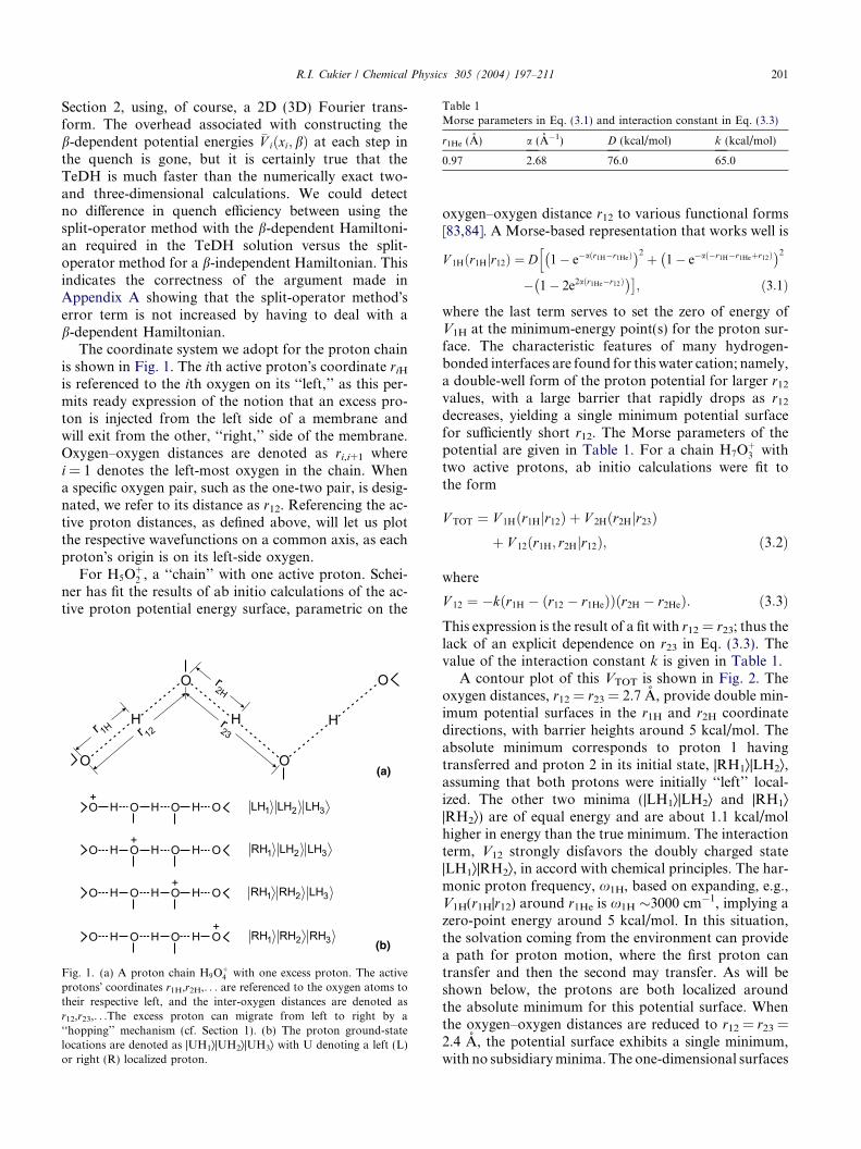
The coordinate system we adopt for the proton chainis shown in Fig. 1. The ith active proton�s coordinate riHis referenced to the ith oxygen on its ‘‘left,’’ as this per-mits ready expression of the notion that an excess pro-ton is injected from the left side of a membrane andwill exit from the other, ‘‘right,’’ side of the membrane.Oxygen–oxygen distances are denoted as ri,i+1 wherei = 1 denotes the left-most oxygen in the chain. Whena specific oxygen pair, such as the one-two pair, is desig-nated, we refer to its distance as r12. Referencing the ac-tive proton distances, as defined above, will let us plotthe respective wavefunctions on a common axis, as eachproton�s origin is on its left-side oxygen.
For H5Oþ2 , a ‘‘chain’’ with one active proton. Schei-
ner has fit the results of ab initio calculations of the ac-tive proton potential energy surface, parametric on the
(a)
(b)
Fig. 1. (a) A proton chain H9Oþ4 with one excess proton. The active
protons� coordinates r1H,r2H,. . . are referenced to the oxygen atoms totheir respective left, and the inter-oxygen distances are denoted asr12,r23,. . .The excess proton can migrate from left to right by a‘‘hopping’’ mechanism (cf. Section 1). (b) The proton ground-statelocations are denoted as |UH1æ|UH2æ|UH3æ with U denoting a left (L)or right (R) localized proton.
oxygen–oxygen distance r12 to various functional forms[83,84]. A Morse-based representation that works well is
V 1Hðr1Hjr12Þ ¼ D 1� e�aðr1H�r1HeÞ� �2 þ 1� e�að�r1H�r1Heþr12Þ
� �2h
� 1� 2e2aðr1He�r12Þ� ��
; ð3:1Þ
where the last term serves to set the zero of energy ofV1H at the minimum-energy point(s) for the proton sur-face. The characteristic features of many hydrogen-bonded interfaces are found for this water cation; namely,a double-well form of the proton potential for larger r12values, with a large barrier that rapidly drops as r12decreases, yielding a single minimum potential surfacefor sufficiently short r12. The Morse parameters of thepotential are given in Table 1. For a chain H7O
þ3 with
two active protons, ab initio calculations were fit tothe form
V TOT ¼ V 1Hðr1Hjr12Þ þ V 2Hðr2Hjr23Þþ V 12ðr1H; r2Hjr12Þ; ð3:2Þ
where
V 12 ¼ �kðr1H � ðr12 � r1HeÞÞðr2H � r2HeÞ: ð3:3ÞThis expression is the result of a fit with r12 = r23; thus thelack of an explicit dependence on r23 in Eq. (3.3). Thevalue of the interaction constant k is given in Table 1.
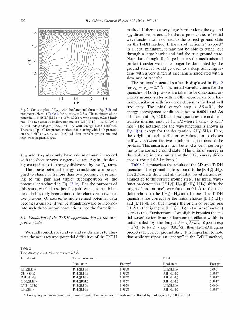
A contour plot of this VTOT is shown in Fig. 2. Theoxygen distances, r12 = r23 = 2.7 A, provide double min-imum potential surfaces in the r1H and r2H coordinatedirections, with barrier heights around 5 kcal/mol. Theabsolute minimum corresponds to proton 1 havingtransferred and proton 2 in its initial state, |RH1æ|LH2æ,assuming that both protons were initially ‘‘left’’ local-ized. The other two minima (|LH1æ|LH2æ and |RH1æ|RH2æ) are of equal energy and are about 1.1 kcal/molhigher in energy than the true minimum. The interactionterm, V12 strongly disfavors the doubly charged state|LH1æ|RH2æ, in accord with chemical principles. The har-monic proton frequency, x1H, based on expanding, e.g.,V1H(r1H|r12) around r1He is x1H �3000 cm�1, implying azero-point energy around 5 kcal/mol. In this situation,the solvation coming from the environment can providea path for proton motion, where the first proton cantransfer and then the second may transfer. As will beshown below, the protons are both localized aroundthe absolute minimum for this potential surface. Whenthe oxygen–oxygen distances are reduced to r12 = r23 =2.4 A, the potential surface exhibits a single minimum,with no subsidiaryminima. The one-dimensional surfaces
1 1.2
1.2
1.4
1.4
1.6
1.6
1.8
1.8
r1H
1
rH2
Fig. 2. Contour plot of VTOT with the functional form in Eq. (3.2) andparameters given in Table 1, for r12 = r23 = 2.7 A. The minimum of thepotential is at |RH1æ |LH2æ = (1.674,1.026) A with energy 0.2265 kcal/mol. The two other subsidiary minima are |LH1æ|LH2æ = (1.033,0.971)A and |RH1æ|RH2æ = (1.729,1.667) A with energy 1.293 kcal/mol.There is a ‘‘path’’ for proton motion that, starting with both protonson the ‘‘left’’ (r1H � r2H � 1.0 A), will first transfer proton one andthen transfer proton two.
202 R.I. Cukier / Chemical Physics 305 (2004) 197–211
V1H and V2H also only have one minimum in accordwith the short oxygen–oxygen distance. Again, the dou-bly charged state is strongly disfavored by the V12 term.
The above potential energy formulation can be ap-plied to chains with more than two protons, by return-ing to the pair and triplet decomposition of thepotential introduced in Eq. (2.1c). For the purposes ofthis work, we shall use just the pair terms, as the ab ini-tio data has only been obtained for chains with two ac-tive protons. Of course, as more refined potential databecomes available, it will be straightforward to incorpo-rate such three-proton correlations into the formalism.
3.1. Validation of the TeDH approximation on the two-
proton chain
We shall consider several r12 and r23 distances to illus-trate the accuracy and potential difficulties of the TeDH
a Energy is given in internal dimensionless units. The conversion to kcal/
method. If there is a very large barrier along the r1H andr2H directions, it could be that a poor choice of initialwavefunction will not lead to the correct ground statefor the TeDH method. If the wavefunction is ‘‘trapped’’in a local minimum, it may not be able to tunnel outthrough a large barrier and find the true ground state.Note that, though, for large barriers the mechanism ofproton transfer would no longer be dominated by theground state; it would go over to a deep tunneling re-gime with a very different mechanism associated with aslow rate of transfer.
The protons� potential surface is displayed in Fig. 2for r12 = r23 = 2.7 A. The initial wavefunctions for thequenches of both protons are taken to be Gaussians; os-cillator ground states with widths appropriate to a har-monic oscillator with frequency chosen as the local wellfrequency. The initial quench step is Db = 0.1, theenergy convergence condition is set to 0.0001 and Dbis halved until Db < 0.01. (These quantities are in dimen-sionless internal units of �hx1H/2 where 1 unit � 5 kcal/mol.) The notation for the wavefunctions is shown inFig. 1(b), except for the designation |SH1æ|SH2æ. Here,the origin of each oscillator wavefunction is chosenhalf-way between the two equilibrium positions of theprotons. This ensures a much better chance of converg-ing to the correct ground state. (The units of energy inthe table are internal units and the 0.127 energy differ-ence is around 0.6 kcal/mol.)
Table 2 summarizes the results of the 2D and TeDHquenches. The ground state is found to be |RH1æ|LH2æ.The 2D results show that all the initial wavefunctions ex-amined go to the correct ground state. The initial wave-function denoted as |L 0H1æ|LH2æ (|L00H1æ|LH2æ) shifts theorigin of proton one�s wavefunction 0.1 A to the right(left), relative to the |LH1æ|LH2æ initial choice. The TeDHquench is not correct for the initial choices |LH1æ|LH2æand |L00H1æ|LH2æ, but moving the origin of proton one0.1 A to the right (the |L 0H1æ|LH2æ initial wavefunction)corrects this. Furthermore, if we slightly broaden the ini-tial wavefunction from its harmonic oscillator width, inunits scaled by the length ‘ ¼
ffiffiffiffiffiffiffiffiffiffiffiffi�h=mx
p, w1(x) � exp
(�x2/2), to w1(x) � exp(�0.8x2/2), then the TeDH againpredicts the correct ground state. It is important to notethat while we report an ‘‘energy’’ in the TeDH method,
R.I. Cukier / Chemical Physics 305 (2004) 197–211 203
it is not an energy in the sense of an eigenstate. The TeDH(and TDH) methods cannot give eigenstate energies.
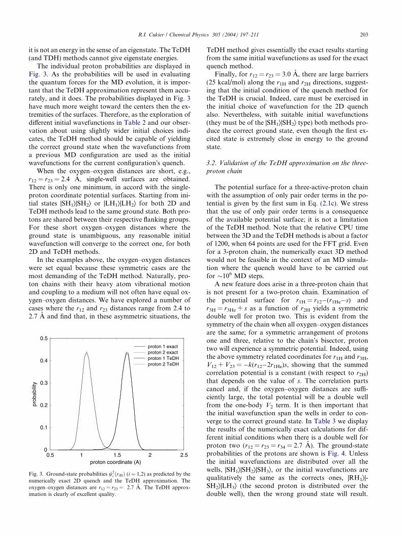
The individual proton probabilities are displayed inFig. 3. As the probabilities will be used in evaluatingthe quantum forces for the MD evolution, it is impor-tant that the TeDH approximation represent them accu-rately, and it does. The probabilities displayed in Fig. 3have much more weight toward the centers then the ex-tremities of the surfaces. Therefore, as the exploration ofdifferent initial wavefunctions in Table 2 and our obser-vation about using slightly wider initial choices indi-cates, the TeDH method should be capable of yieldingthe correct ground state when the wavefunctions froma previous MD configuration are used as the initialwavefunctions for the current configuration�s quench.
When the oxygen–oxygen distances are short, e.g.,r12 = r23 = 2.4 A, single-well surfaces are obtained.There is only one minimum, in accord with the single-proton coordinate potential surfaces. Starting from ini-tial states |SH1æ|SH2æ or |LH1æ|LH2æ for both 2D andTeDH methods lead to the same ground state. Both pro-tons are shared between their respective flanking groups.For these short oxygen–oxygen distances where theground state is unambiguous, any reasonable initialwavefunction will converge to the correct one, for both2D and TeDH methods.
In the examples above, the oxygen–oxygen distanceswere set equal because these symmetric cases are themost demanding of the TeDH method. Naturally, pro-ton chains with their heavy atom vibrational motionand coupling to a medium will not often have equal ox-ygen–oxygen distances. We have explored a number ofcases where the r12 and r23 distances range from 2.4 to2.7 A and find that, in these asymmetric situations, the
Fig. 3. Ground-state probabilities w2i ðriHÞ (i = 1,2) as predicted by the
numerically exact 2D quench and the TeDH approximation. Theoxygen–oxygen distances are r12 = r23 = 2.7 A. The TeDH approx-imation is clearly of excellent quality.
TeDH method gives essentially the exact results startingfrom the same initial wavefunctions as used for the exactquench method.
Finally, for r12 = r23 = 3.0 A, there are large barriers(25 kcal/mol) along the r1H and r2H directions, suggest-ing that the initial condition of the quench method forthe TeDH is crucial. Indeed, care must be exercised inthe initial choice of wavefunction for the 2D quenchalso. Nevertheless, with suitable initial wavefunctions(they must be of the |SH1æ|SH2æ type) both methods pro-duce the correct ground state, even though the first ex-cited state is extremely close in energy to the groundstate.
3.2. Validation of the TeDH approximation on the three-
proton chain
The potential surface for a three-active-proton chainwith the assumption of only pair order terms in the po-tential is given by the first sum in Eq. (2.1c). We stressthat the use of only pair order terms is a consequenceof the available potential surface; it is not a limitationof the TeDH method. Note that the relative CPU timebetween the 3D and the TeDH methods is about a factorof 1200, when 64 points are used for the FFT grid. Evenfor a 3-proton chain, the numerically exact 3D methodwould not be feasible in the context of an MD simula-tion where the quench would have to be carried outfor �106 MD steps.
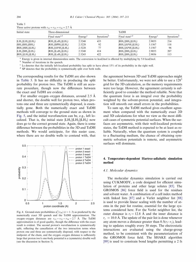
A new feature does arise in a three-proton chain thatis not present for a two-proton chain. Examination ofthe potential surface for r1H = r12�(r1He�s) andr3H = r3He + s as a function of r2H yields a symmetricdouble well for proton two. This is evident from thesymmetry of the chain when all oxygen–oxygen distancesare the same; for a symmetric arrangement of protonsone and three, relative to the chain�s bisector, protontwo will experience a symmetric potential. Indeed, usingthe above symmetry related coordinates for r1H and r3H,V12 + V23 = �k(r12�2r1He)s, showing that the summedcorrelation potential is a constant (with respect to r2H)that depends on the value of s. The correlation partscancel and, if the oxygen–oxygen distances are suffi-ciently large, the total potential will be a double wellfrom the one-body V2 term. It is then important thatthe initial wavefunction span the wells in order to con-verge to the correct ground state. In Table 3 we displaythe results of the numerically exact calculations for dif-ferent initial conditions when there is a double well forproton two (r12 = r23 = r34 = 2.7 A). The ground-stateprobabilities of the protons are shown is Fig. 4. Unlessthe initial wavefunctions are distributed over all thewells, |SH1æ|SH2æ|SH3æ, or the initial wavefunctions arequalitatively the same as the corrects ones, |RH1æ|-SH2æ|LH3æ (the second proton is distributed over thedouble well), then the wrong ground state will result.
Table 3Three active protons with r12 = r23 = r34 = 2.7 A
Initial state Three-dimensional TeDH
Final statec,d Energya Iterationsb Final statec,d Energya Iterationsb
a Energy is given in internal dimensionless units. The conversion to kcal/mol is effected by multiplying by 5.0 kcal/mol.b Number of iterations in the quench.c Ls denotes that the initially left-localized probability has split to have about 15% of its probability in the right well.d SP denotes that the probability is symmetrically split over both wells.
204 R.I. Cukier / Chemical Physics 305 (2004) 197–211
The corresponding results for the TeDH are also shownin Table 3. It has no difficulty in producing the splitprobability for proton two. The TeDH is still an accu-rate procedure, though now the differences betweenthe exact and TeDH are evident.
For smaller oxygen–oxygen distances, around 2.5 Aand shorter, the double well for proton two, when pro-tons one and three are symmetrically disposed, is essen-tially gone. Both the numerically exact and TeDHmethods will converge to the ground state as shown inFig. 5, and the initial wavefunction can be, e.g., left lo-calized. That is, the initial state |LH1æ|LH2æ|LH3æ nowdoes go to the correct ground state. Again, there is somedifference between the probabilities in the 3D and TeDHmethods. We would anticipate, for this easier case,where there are no double wells to contend with, that
Fig. 4. Ground-state probabilities w2i ðriHÞ (i = 1–3) as predicted by the
numerically exact 3D quench and the TeDH approximation. Theoxygen–oxygen distances are r12 = r23 = r34 = 2.7 A. The TeDHapproximation is of good quality, though the difference with the exactresult is evident. The second proton�s wavefunction is symmetricallysplit, reflecting the cancellation of the two interaction terms whenproton one and three are symmetrically disposed, with respect to themidpoint of the chain, and the oxygen–oxygen distance is sufficientlylarge that proton two�s one-body potential is a (symmetric) double well(see the discussion in Section 3).
the agreement between 3D and TeDH approaches mightbe better. Unfortunately, we were not able to use a 1283
grid for the 3D calculation, as the memory requirementswere too large. However, the agreement certainly is suf-ficiently good to consider the method reliable. Note thatthe quantum force is an integral over the probabilityweighted by the solvent-proton potential, and integra-tion will smooth out small errors in the probabilities.
To sum up, the TeDH method gives excellent agree-ment when compared with the numerically exact 2Dand 3D calculations for what we view as the most diffi-cult cases of symmetric potential surfaces. When the sur-faces are asymmetric, with their well-localized protonicstates, the TeDH method is expected to be at least as re-liable. Naturally, when the quantum system is coupledto a fluctuating medium, the chance of obtaining sym-metric solvation potentials is remote, and asymmetricsurfaces will dominate.
The molecular dynamics simulation is carried outusing CUKMODY, a code designed for efficient simu-lation of proteins and other large solutes [85]. TheGROMOS [86] force field is used for the residuesand solvent water. A combination of a cell index methodwith linked lists [87] and a Verlet neighbor list [88]is used to provide linear scaling with the number of at-oms in the pair list routine, essential for the large sys-tems considered here. For the Verlet neighbor list, theouter distance is rl = 12.8 A and the inner distance isrc = 10.0 A. The update of the pair list is done wheneverany atom moves a distance greater than 0.5(rl�rc), lead-ing to updates roughly every 30 steps. The electrostaticinteractions are evaluated using the charge-groupmethod, to be consistent with the parameterization ofthe GROMOS force field. The SHAKE algorithm[89] is used to constrain bond lengths permitting a 2 fs
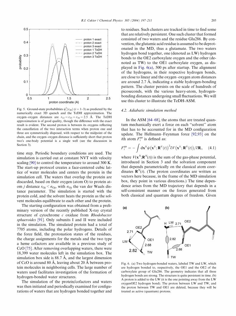
Fig. 6. (a) Two hydrogen-bonded waters, labeled TW and LW, whichare hydrogen bonded to, respectively, the OE1 and the OE2 of thecarboxylate group of Glu286. The geometry indicates that all threehydrogen bonds are strong. The structure is quite persistent in time. (b)A proton is added to the LW (it is the one pointing away from the LWoxygenOE2 hydrogen bond). The proton between LW and TW, andthe proton between TW and OE1 are deleted, because they will betreated as active (quantum) protons.
Fig. 5. Ground-state probabilities w2i ðriHÞ (i = 1–3) as predicted by the
numerically exact 3D quench and the TeDH approximation. Theoxygen–oxygen distances are r12 = r23 = r34 = 2.5 A. The TeDHapproximation is of good quality, though the difference with the exactresult is evident. The second proton is between its oxygens reflectingthe cancellation of the two interaction terms when proton one andthree are symmetrically disposed, with respect to the midpoint of thechain, and the oxygen–oxygen distance is sufficiently short that protontwo�s one-body potential is a single well (see the discussion inSection 3).
R.I. Cukier / Chemical Physics 305 (2004) 197–211 205
time step. Periodic boundary conditions are used. Thesimulation is carried out at constant NVT with velocityscaling [90] to control the temperature to around 300 K.The start-up protocol creates a face-centered cubic lat-tice of water molecules and centers the protein in thesimulation cell. The waters that overlap the protein arediscarded, based on their oxygen (atom O) to protein at-om j distance rOj < rOj, with rOj the van der Waals dis-tance parameter. The simulation is started with theprotein cold, and the solvent heats the protein as the sol-vent molecules equilibrate to each other and the protein.
The starting configuration was obtained from a preli-minary version of the recently published X-ray crystalstructure of cytochrome c oxidase from Rhodobactersphaeroides [91]. Only subunits I and II were includedin the simulation. The simulated protein had a total of7705 atoms, including the polar hydrogens. Details ofthe force field, the protonation states of the residues,the charge assignments for the metals and the two typea heme cofactors are available in a previous study ofCcO [75]. After removing overlapping waters, there were18,399 water molecules left in the simulation box. Thesimulation box side is 88.7 A, and the largest dimensionof CcO is around 80 A, leaving about 20 A between pro-tein molecules in neighboring cells. The large number ofwaters used facilitates investigation of the formation ofhydrogen-bonded water structures.
The simulation of the protein/cofactors and waterswas then initiated and periodically examined for configu-rations of waters that are hydrogen bonded together and
to residues. Such clusters are tracked in time to find somethat are relatively persistent. One such cluster that formedconsisted of two waters and the residue Glu286. By con-vention, the glutamic acid residue is assumed tobedeprot-onated in the MD, thus a glutamate. The two watershydrogen bond together, one (denoted as LW) hydrogenbonds to the OE2 carboxylate oxygen and the other (de-noted as TW) to the OE1 carboxylate oxygen, as dis-played in Fig. 6(a), 500 ps after startup. The alignmentof the hydrogens, in their respective hydrogen bonds,are close to linear and the oxygen–oxygen atom distancesare around 2.7 A, indicating a stable hydrogen-bondingpattern. The cluster persists on the scale of hundreds ofpicoseconds, with the various heavy-atom, hydrogen-bonding distances undergoing small fluctuations. We willuse this cluster to illustrate the TeDH-ASM.
4.2. Adiabatic simulation method
In the ASM [64–68], the atoms that are treated quan-tum mechanically exert a force on each ‘‘solvent’’ atomthat has to be accounted for in the MD configurationupdate. The Hellmann–Feynman force [92,93] on theith atom F qu
i is defined as:
F qui ¼ �
ZdxNw xN ;RN ðtÞ
� �2oV xN ;RN ðtÞ
� �=oRi; ð4:1Þ
where V(xN;RN(t)) is the sum of the gas-phase potential,introduced in Section 3 and the solvation componentthat depends parametrically on the classical atom coor-dinates RN(t). (The proton coordinates are written asvectors here because, in the frame of the MD simulationbox, they point in various directions.) The time depen-dence arises from the MD trajectory that depends in aself-consistent manner on the forces generated fromboth classical and quantum degrees of freedom. Given
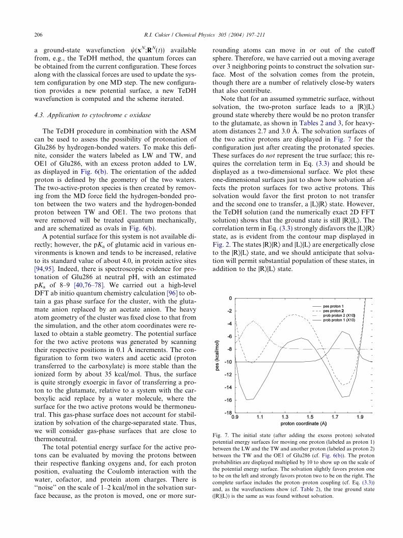
Fig. 7. The initial state (after adding the excess proton) solvatedpotential energy surfaces for moving one proton (labeled as proton 1)between the LW and the TW and another proton (labeled as proton 2)between the TW and the OE1 of Glu286 (cf. Fig. 6(b)). The protonprobabilities are displayed multiplied by 10 to show up on the scale ofthe potential energy surface. The solvation slightly favors proton oneto be on the left and strongly favors proton two to be on the right. Thecomplete surface includes the proton–proton coupling (cf. Eq. (3.3))and, as the wavefunctions show (cf. Table 2), the true ground state(|Ræ|Læ) is the same as was found without solvation.
206 R.I. Cukier / Chemical Physics 305 (2004) 197–211
a ground-state wavefunction w(xN;RN(t)) availablefrom, e.g., the TeDH method, the quantum forces canbe obtained from the current configuration. These forcesalong with the classical forces are used to update the sys-tem configuration by one MD step. The new configura-tion provides a new potential surface, a new TeDHwavefunction is computed and the scheme iterated.
4.3. Application to cytochrome c oxidase
The TeDH procedure in combination with the ASMcan be used to assess the possibility of protonation ofGlu286 by hydrogen-bonded waters. To make this defi-nite, consider the waters labeled as LW and TW, andOE1 of Glu286, with an excess proton added to LW,as displayed in Fig. 6(b). The orientation of the addedproton is defined by the geometry of the two waters.The two-active-proton species is then created by remov-ing from the MD force field the hydrogen-bonded pro-ton between the two waters and the hydrogen-bondedproton between TW and OE1. The two protons thatwere removed will be treated quantum mechanically,and are schematized as ovals in Fig. 6(b).
A potential surface for this system is not available di-rectly; however, the pKa of glutamic acid in various en-vironments is known and tends to be increased, relativeto its standard value of about 4.0, in protein active sites[94,95]. Indeed, there is spectroscopic evidence for pro-tonation of Glu286 at neutral pH, with an estimatedpKa of 8–9 [40,76–78]. We carried out a high-levelDFT ab initio quantum chemistry calculation [96] to ob-tain a gas phase surface for the cluster, with the gluta-mate anion replaced by an acetate anion. The heavyatom geometry of the cluster was fixed close to that fromthe simulation, and the other atom coordinates were re-laxed to obtain a stable geometry. The potential surfacefor the two active protons was generated by scanningtheir respective positions in 0.1 A increments. The con-figuration to form two waters and acetic acid (protontransferred to the carboxylate) is more stable than theionized form by about 35 kcal/mol. Thus, the surfaceis quite strongly exoergic in favor of transferring a pro-ton to the glutamate, relative to a system with the car-boxylic acid replace by a water molecule, where thesurface for the two active protons would be thermoneu-tral. This gas-phase surface does not account for stabil-ization by solvation of the charge-separated state. Thus,we will consider gas-phase surfaces that are close tothermoneutral.
The total potential energy surface for the active pro-tons can be evaluated by moving the protons betweentheir respective flanking oxygens and, for each protonposition, evaluating the Coulomb interaction with thewater, cofactor, and protein atom charges. There is‘‘noise’’ on the scale of 1–2 kcal/mol in the solvation sur-face because, as the proton is moved, one or more sur-
rounding atoms can move in or out of the cutoffsphere. Therefore, we have carried out a moving averageover 3 neighboring points to construct the solvation sur-face. Most of the solvation comes from the protein,though there are a number of relatively close-by watersthat also contribute.
Note that for an assumed symmetric surface, withoutsolvation, the two-proton surface leads to a |Ræ|Læground state whereby there would be no proton transferto the glutamate, as shown in Tables 2 and 3, for heavy-atom distances 2.7 and 3.0 A. The solvation surfaces ofthe two active protons are displayed in Fig. 7 for theconfiguration just after creating the protonated species.These surfaces do not represent the true surface; this re-quires the correlation term in Eq. (3.3) and should bedisplayed as a two-dimensional surface. We plot theseone-dimensional surfaces just to show how solvation af-fects the proton surfaces for two active protons. Thissolvation would favor the first proton to not transferand the second one to transfer, a |Læ|Ræ state. However,the TeDH solution (and the numerically exact 2D FFTsolution) shows that the ground state is still |Ræ|Læ. Thecorrelation term in Eq. (3.3) strongly disfavors the |Læ|Ræstate, as is evident from the contour map displayed inFig. 2. The states |Ræ|Ræ and |Læ|Læ are energetically closeto the |Ræ|Læ state, and we should anticipate that solva-tion will permit substantial population of these states, inaddition to the |Ræ|Læ state.
R.I. Cukier / Chemical Physics 305 (2004) 197–211 207
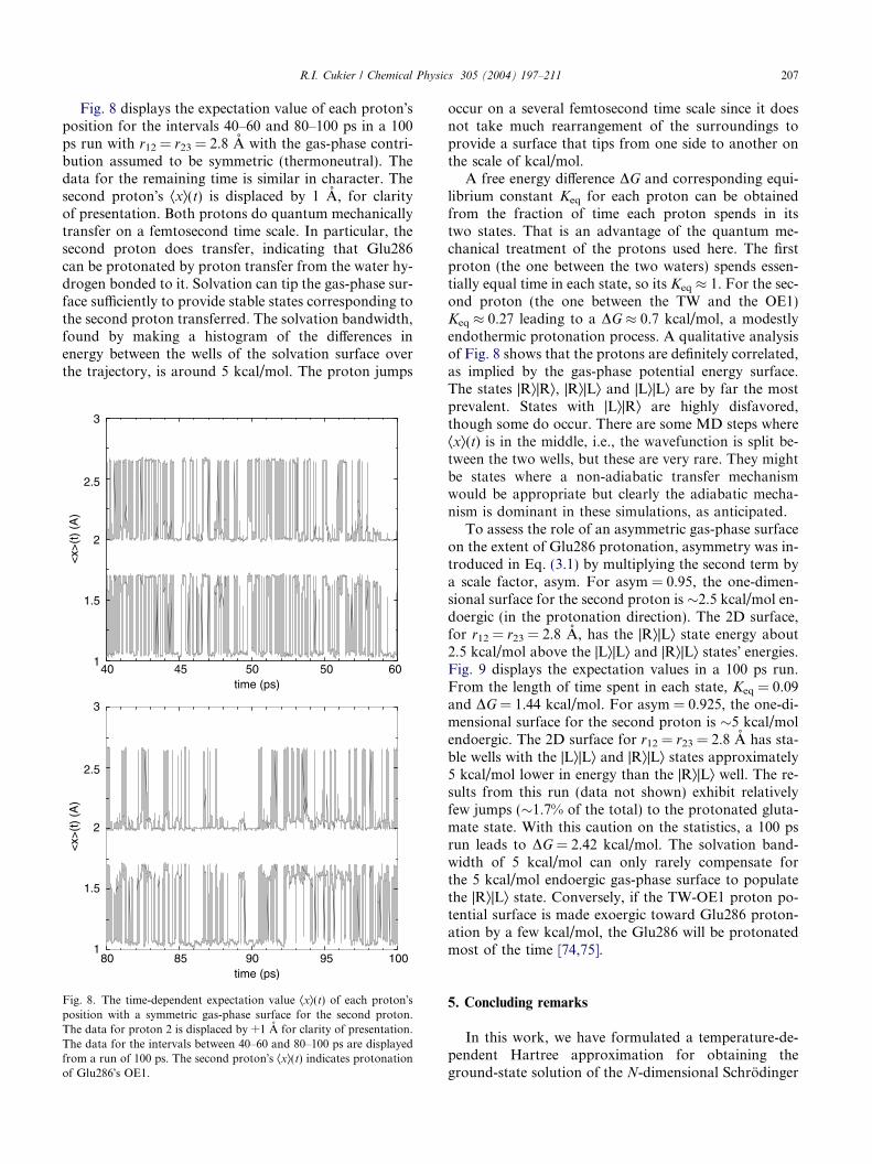
Fig. 8 displays the expectation value of each proton�sposition for the intervals 40–60 and 80–100 ps in a 100ps run with r12 = r23 = 2.8 A with the gas-phase contri-bution assumed to be symmetric (thermoneutral). Thedata for the remaining time is similar in character. Thesecond proton�s Æxæ(t) is displaced by 1 A, for clarityof presentation. Both protons do quantum mechanicallytransfer on a femtosecond time scale. In particular, thesecond proton does transfer, indicating that Glu286can be protonated by proton transfer from the water hy-drogen bonded to it. Solvation can tip the gas-phase sur-face sufficiently to provide stable states corresponding tothe second proton transferred. The solvation bandwidth,found by making a histogram of the differences inenergy between the wells of the solvation surface overthe trajectory, is around 5 kcal/mol. The proton jumps
85 90 9580 100time (ps)
45 50 5040 60time (ps)
1
1.5
2
2.5
3
<x>
(t)
(A)
1
1.5
2
2.5
3
<x>
(t)
(A)
Fig. 8. The time-dependent expectation value Æxæ(t) of each proton�sposition with a symmetric gas-phase surface for the second proton.The data for proton 2 is displaced by +1 A for clarity of presentation.The data for the intervals between 40–60 and 80–100 ps are displayedfrom a run of 100 ps. The second proton�s Æxæ(t) indicates protonationof Glu286�s OE1.
occur on a several femtosecond time scale since it doesnot take much rearrangement of the surroundings toprovide a surface that tips from one side to another onthe scale of kcal/mol.
A free energy difference DG and corresponding equi-librium constant Keq for each proton can be obtainedfrom the fraction of time each proton spends in itstwo states. That is an advantage of the quantum me-chanical treatment of the protons used here. The firstproton (the one between the two waters) spends essen-tially equal time in each state, so its Keq � 1. For the sec-ond proton (the one between the TW and the OE1)Keq � 0.27 leading to a DG � 0.7 kcal/mol, a modestlyendothermic protonation process. A qualitative analysisof Fig. 8 shows that the protons are definitely correlated,as implied by the gas-phase potential energy surface.The states |Ræ|Ræ, |Ræ|Læ and |Læ|Læ are by far the mostprevalent. States with |Læ|Ræ are highly disfavored,though some do occur. There are some MD steps whereÆxæ(t) is in the middle, i.e., the wavefunction is split be-tween the two wells, but these are very rare. They mightbe states where a non-adiabatic transfer mechanismwould be appropriate but clearly the adiabatic mecha-nism is dominant in these simulations, as anticipated.
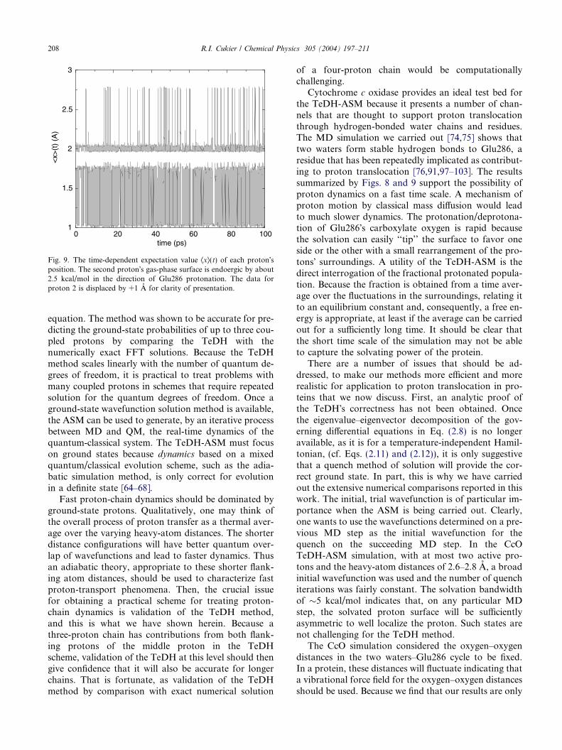
To assess the role of an asymmetric gas-phase surfaceon the extent of Glu286 protonation, asymmetry was in-troduced in Eq. (3.1) by multiplying the second term bya scale factor, asym. For asym = 0.95, the one-dimen-sional surface for the second proton is �2.5 kcal/mol en-doergic (in the protonation direction). The 2D surface,for r12 = r23 = 2.8 A, has the |Ræ|Læ state energy about2.5 kcal/mol above the |Læ|Læ and |Ræ|Læ states� energies.Fig. 9 displays the expectation values in a 100 ps run.From the length of time spent in each state, Keq = 0.09and DG = 1.44 kcal/mol. For asym = 0.925, the one-di-mensional surface for the second proton is �5 kcal/molendoergic. The 2D surface for r12 = r23 = 2.8 A has sta-ble wells with the |Læ|Læ and |Ræ|Læ states approximately5 kcal/mol lower in energy than the |Ræ|Læ well. The re-sults from this run (data not shown) exhibit relativelyfew jumps (�1.7% of the total) to the protonated gluta-mate state. With this caution on the statistics, a 100 psrun leads to DG = 2.42 kcal/mol. The solvation band-width of 5 kcal/mol can only rarely compensate forthe 5 kcal/mol endoergic gas-phase surface to populatethe |Ræ|Læ state. Conversely, if the TW-OE1 proton po-tential surface is made exoergic toward Glu286 proton-ation by a few kcal/mol, the Glu286 will be protonatedmost of the time [74,75].
5. Concluding remarks
In this work, we have formulated a temperature-de-pendent Hartree approximation for obtaining theground-state solution of the N-dimensional Schrodinger
0 20 40 60 80 100time (ps)
1
1.5
2
2.5
3
<x>
(t)
(A)
Fig. 9. The time-dependent expectation value Æxæ(t) of each proton�sposition. The second proton�s gas-phase surface is endoergic by about2.5 kcal/mol in the direction of Glu286 protonation. The data forproton 2 is displaced by +1 A for clarity of presentation.
208 R.I. Cukier / Chemical Physics 305 (2004) 197–211
equation. The method was shown to be accurate for pre-dicting the ground-state probabilities of up to three cou-pled protons by comparing the TeDH with thenumerically exact FFT solutions. Because the TeDHmethod scales linearly with the number of quantum de-grees of freedom, it is practical to treat problems withmany coupled protons in schemes that require repeatedsolution for the quantum degrees of freedom. Once aground-state wavefunction solution method is available,the ASM can be used to generate, by an iterative processbetween MD and QM, the real-time dynamics of thequantum-classical system. The TeDH-ASM must focuson ground states because dynamics based on a mixedquantum/classical evolution scheme, such as the adia-batic simulation method, is only correct for evolutionin a definite state [64–68].
Fast proton-chain dynamics should be dominated byground-state protons. Qualitatively, one may think ofthe overall process of proton transfer as a thermal aver-age over the varying heavy-atom distances. The shorterdistance configurations will have better quantum over-lap of wavefunctions and lead to faster dynamics. Thusan adiabatic theory, appropriate to these shorter flank-ing atom distances, should be used to characterize fastproton-transport phenomena. Then, the crucial issuefor obtaining a practical scheme for treating proton-chain dynamics is validation of the TeDH method,and this is what we have shown herein. Because athree-proton chain has contributions from both flank-ing protons of the middle proton in the TeDHscheme, validation of the TeDH at this level should thengive confidence that it will also be accurate for longerchains. That is fortunate, as validation of the TeDHmethod by comparison with exact numerical solution
of a four-proton chain would be computationallychallenging.
Cytochrome c oxidase provides an ideal test bed forthe TeDH-ASM because it presents a number of chan-nels that are thought to support proton translocationthrough hydrogen-bonded water chains and residues.The MD simulation we carried out [74,75] shows thattwo waters form stable hydrogen bonds to Glu286, aresidue that has been repeatedly implicated as contribut-ing to proton translocation [76,91,97–103]. The resultssummarized by Figs. 8 and 9 support the possibility ofproton dynamics on a fast time scale. A mechanism ofproton motion by classical mass diffusion would leadto much slower dynamics. The protonation/deprotona-tion of Glu286�s carboxylate oxygen is rapid becausethe solvation can easily ‘‘tip’’ the surface to favor oneside or the other with a small rearrangement of the pro-tons� surroundings. A utility of the TeDH-ASM is thedirect interrogation of the fractional protonated popula-tion. Because the fraction is obtained from a time aver-age over the fluctuations in the surroundings, relating itto an equilibrium constant and, consequently, a free en-ergy is appropriate, at least if the average can be carriedout for a sufficiently long time. It should be clear thatthe short time scale of the simulation may not be ableto capture the solvating power of the protein.
There are a number of issues that should be ad-dressed, to make our methods more efficient and morerealistic for application to proton translocation in pro-teins that we now discuss. First, an analytic proof ofthe TeDH�s correctness has not been obtained. Oncethe eigenvalue–eigenvector decomposition of the gov-erning differential equations in Eq. (2.8) is no longeravailable, as it is for a temperature-independent Hamil-tonian, (cf. Eqs. (2.11) and (2.12)), it is only suggestivethat a quench method of solution will provide the cor-rect ground state. In part, this is why we have carriedout the extensive numerical comparisons reported in thiswork. The initial, trial wavefunction is of particular im-portance when the ASM is being carried out. Clearly,one wants to use the wavefunctions determined on a pre-vious MD step as the initial wavefunction for thequench on the succeeding MD step. In the CcOTeDH-ASM simulation, with at most two active pro-tons and the heavy-atom distances of 2.6–2.8 A, a broadinitial wavefunction was used and the number of quenchiterations was fairly constant. The solvation bandwidthof �5 kcal/mol indicates that, on any particular MDstep, the solvated proton surface will be sufficientlyasymmetric to well localize the proton. Such states arenot challenging for the TeDH method.
The CcO simulation considered the oxygen–oxygendistances in the two waters–Glu286 cycle to be fixed.In a protein, these distances will fluctuate indicating thata vibrational force field for the oxygen–oxygen distancesshould be used. Because we find that our results are only
R.I. Cukier / Chemical Physics 305 (2004) 197–211 209
modestly dependent on these distances, introduction ofthese effects should not lead to substantial modifica-tions. However, the motion of the waters after proton-ation is an important issue to address. The addition ofthe excess proton and the switch from the MD forcefield to the quantum treatment of the active protonschanges the forces and may well lead to the cycle break-ing up, or adding additional water molecules. Indeed, inorder for proton translocation to proceed, such eventsmust occur. That is why we did not attempt to formulatea rate constant for the protonation process. Clearly,protonation of a water/residue cycle, or other structuresthat form, must lead to new geometric configurationsthat can pass protons across the membrane.
Acknowledgement
The financial support of the National Institutes ofHealth (GM62790) is gratefully acknowledged. We areindebted to Professor S. Ferguson-Miller for providingthe coordinates of Rhodobacter sphaeroides used in thesimulation of CcO, to members of her group (Dr. D.Mills and Mr. B. Schmidt) and to Dr. S. Seibold for helpin preparing the CcO input file, and to all of them fornumerous enlightening discussions about CcO.
Appendix A. The time-dependent Hartree approxima-tion to the Schrodinger equation for any of the degreesof freedom is
i�houðx; tÞ
ot¼ Hðx; tÞuðx; tÞ: ðA:1Þ
We shall use the more conventional time version for thisanalysis and obtain the temperature version by the sub-stitution, t = �ib�h. As a reminder of the operator natureof the Hamiltonian, we use aˆon it. In contrast with theexact Schrodinger equation with its time-independent H,the propagator U(t,t0) must be expressed as an orderedexponential
Uðt; t0Þ ¼ Tþe�iR t
t0dsHðsÞ
� 1þ ð�iÞZ t
t0
dsHðsÞ þ ð�iÞ2Z t
t0
ds1
�Z s1
t0
d2Hðs1ÞHðs2Þ þ � � � ðA:2Þ
that is properly time ordered because s2 < s1. The issuehere is to assess the error made in using the Trotter for-mula in the form of the second-order, split-exponentialoperator formula. If the error is no worse than the0(Dt)3 error of this split-operator formula for a time-in-dependent Hamiltonian [79–82], then we anticipate thatthe method will be a fast and reliable method to obtainthe ground-state wavefunction.
For the step from t0 ! t0 + Dt, we may write a sec-ond-order midstep expression,
with t0 < s < t0 + Dt. Using this expression in Eq. (A.1)and evaluating all the terms shows that the error termis still of 0(Dt)3 and is the same error as for a time-inde-pendent H. The non-commutativity arising from thetime-dependent Hamiltonian, [H(s1), H(s2)] 6¼ 0;(s1 6¼ s2), does not contribute to the error to 0(Dt)3. An-other approach is to expand about t0 the beginning ofthe interval. When this is done, the error term isHðt0Þ _Hðt0ÞðDtÞ3, and is of the same order as that ofthe time-independent, split-operator form. While ahalf-step formalism for the split-operator method canbe developed, the overhead incurred in such a formulaseems not to be worth the effort, because the error ofthe standard split-operator formula arising from thenon-commutativity ½T ; V � 6¼ 0 is of the same order asthat incurred in the H(t) case with expansion about t0.Unless there was an unfavorable numerical coefficientthat would significantly reduce its accuracy, the aboveerror estimate indicates that the expansion about t0should be used, and we do so in this work. Thus, aworking formula for a Hamiltonian schematized asHðtÞ ¼ T þ V 0 þ �V ðtÞ, based on Eq. (A.1) and the aboveconsiderations is
As the wavefunction is known at time t0, the expectationvalue �V ðt0Þ is available to propagate to t0 + Dt. The sub-stitution t = �ib�h then yields Eq. (2.13).
References
[1] D. Voet, J.G. Voet, Biochemistry, John Wiley & Sons, NewYork, 2004.
[2] J.F. Nagle, S. Tristam-Nagle, J. Membr. Biol. 74 (1983) 1.[3] N. Agmon, Chem. Phys. Lett. 244 (1995) 456.[4] R.A. Mathies, S.W. Lin, J.B. Ames, W.T. Pollard, Annu. Rev.
Biophys. Chem. 20 (1991) 491.[5] M.Y. Okamura, G. Feher, Annu. Rev. Biochem. 61 (1992) 861.[6] L. Baciou, H. Michel, Biochemistry 34 (1995) 7967.[7] S. Ferguson-Miller, G.T. Babcock, Chem. Rev. 96 (1996) 2889.[8] M. Wikstrom, Bba-Bioenergetics 1458 (2000) 188.[9] P. Brzezinski, G. Larsson, Bba-Bioenergetics 1605 (2003) 1.[10] A. Warshel, J. Phys. Chem. 86 (1982) 2218.[11] D. Borgis, G. Tarjus, H. Azzouz, J. Phys. Chem. 96 (1992) 3188.[12] H. Azzouz, D. Borgis, J. Chem. Phys. 98 (1993) 7361.
210 R.I. Cukier / Chemical Physics 305 (2004) 197–211
[14] P. Bala, B. Lesyng, J.A. McCammon, Chem. Phys. 180 (1994)271.
[15] S. Hammes-Schiffer, J.C. Tully, J. Phys. Chem. 99 (1995) 5793.[16] J.-Y. Fang, S. Hammes-Schiffer, J. Chem. Phys. 107 (1997) 5727.[17] D. Laria, R. Kapral, D. Estrin, G. Ciccotti, J. Chem. Phys. 104
(1996) 6560.[18] S. Consta, R. Kapral, J. Chem. Phys. 101 (1994) 10908.[19] A. Staib, D. Borgis, J. Chem. Phys. 103 (1995) 2642.[20] J. Mavri, H.J.C. Berendsen, W.Fv. Gunsteren, J. Phys. Chem. 97
(1993) 13469.[21] D. VanDerSpoel, H.J.C. Berendsen, J. Phys. Chem. 100 (1996)
2535.[22] J. Lobaugh, G.A. Voth, J. Chem. Phys. 104 (1996) 2056.[23] M. Pavese, S. Chawla, D. Lu, J. Lobaugh, G.A. Voth, J. Chem.
Phys. 107 (1997) 7428.[24] K. Ando, J.T. Hynes, J. Phys. Chem. B 101 (1997) 10464.[25] R.I. Cukier, J. Zhu, J. Phys. Chem. 101 (1997) 7180.[26] R.I. Cukier, J. Zhu, J. Chem. Phys. 110 (1999) 9587.[27] S. Hammes-Schiffer, S.R. Billeter, Int. Rev. Phys. Chem. 20
(2001) 591.[28] M.L. Brewer, U.W. Schmitt, G.A. Voth, Biophys. J. 80 (2001)
1691.[29] M.A. Lill, V. Helms, Proc. Natl. Acad. Sci. USA 99 (2002) 2778.[30] R. Pomes, B. Roux, Biophys. J. 82 (2002) 2304.[31] B. Roux, Acc. Chem. Res. 35 (2002) 366.[32] G.A. Voth, Front. Biosci. 8 (2003) S1384.[33] R. Pomes, C.H. Yu, Front. Biosci. 8 (2003) D1288.[34] V. Zoete, M. Meuwly, J. Chem. Phys. 120 (2004) 7085.[35] Y.J. Wu, G.A. Voth, Biophys. J. 85 (2003) 864.[36] J. Lobaugh, G.A. Voth, J. Chem. Phys. 100 (1994) 3039.[37] J.-K. Hwang, A. Warshel, J. Phys. Chem. 97 (1993) 10053.[38] R. Pomes, B. Roux, J. Phys. Chem. 100 (1996) 2519.[39] J. Cao, G.A. Voth, J. Chem. Phys. 99 (1993) 1070.[40] J. Cao, G.A. Voth, J. Chem. Phys. 100 (1994) 5106.[41] U.W. Schmitt, G.A. Voth, J. Chem. Phys. 111 (1999) 9361.[42] Y. Ohta, K. Ohta, K. Kinugawa, Int. J. Quantum Chem. 95
(2003) 372.[43] H. Decornez, K. Drukker, M.M. Hurley, S. Hammes-Schiffer,
Ber. Bunsenges. Phys. Chem. 102 (1998) 533.[44] A.B. McCoy, R.B. Gerber, M.A. Ratner, J. Chem. Phys. 101
(1994) 1975.[45] N. Makri, W.H. Miller, J. Chem. Phys. 87 (1987) 5781.[46] U. Manthe, H.-D. Meyer, L.S. Cederbaum, J. Chem. Phys. 97
(1992) 3199.[47] F.A. Bornemann, P. Nattesheim, C. Schutte, J. Chem. Phys. 105
(1996) 1074.[48] J. Wilkie, M.A. Ratner, R.B. Gerber, J. Chem. Phys. 110 (1999)
7610.[49] H.D. Meyer, G.A. Worth, Theor. Chem. Acc. 109 (2003) 251.[50] R. Pomes, B. Roux, Chem. Phys. Lett. 234 (1995) 416.[51] J.-Y. Fang, S. Hammes-Schiffer, J. Chem. Phys. 106 (1997) 8442.[52] S. Hammes-Schiffer, J. Chem. Phys. 105 (1996) 2236.[53] K. Drukker, S. Hammes-Schiffer, J. Chem. Phys. 107 (1997) 363.[54] K. Drukker, S.Wd. Leeuw, S. Hammes-Schiffer, J. Chem. Phys.
108 (1998) 6799.[55] K. Laasonen, M. Sprik, M. Parrinello, R. Car, J. Chem. Phys.
99 (1993) 9081.[56] M. Sprik, J. Hutter, M. Parrinello, J. Chem. Phys. 105 (1996)
1142.[57] M.E. Tuckerman, K. Laasonen, M. Sprik, M. Parrinello, J.
Chem. Phys. 103 (1995) 150.[58] M.E. Tuckerman, K. Laasonen, M. Sprik, M. Parrinello, J.
Phys. Chem. 99 (1995) 5749.[59] D.E. Sagnella, K. Laasonen, M.L. Klein, Biophys. J. 71 (1996)
1172.
[60] H.S. Mei, M.E. Tuckerman, D.E. Sagnella, M.L. Klein, J. Phys.Chem. B 102 (1998) 10466.
[61] R. Car, M. Parrinello, Phys. Rev. Lett. 55 (1985) 2471.[62] M.E. Tuckerman, J. Phys. Condens. Matter 14 (2002) R1297.[63] R.P. Feynman, A. Hibbs, Quantum Mechanics and Path
Integrals, McGraw-Hill, New York, 1965.[64] A. Selloni, P. Carnevali, R. Car, M. Parrinello, Phys. Rev. Lett.
59 (1987) 823.[65] R.N. Barnett, U. Landman, A. Nitzan, J. Chem. Phys. 89 (1988)
2242.[66] P.J. Rossky, J. Schnitker, J. Phys. Chem. 92 (1988) 4277.[67] S.-Y. Sheu, R.I. Cukier, J. Chem. Phys. 94 (1991) 8258.[68] J. Zhu, R.I. Cukier, J. Chem. Phys. 98 (1993) 5679.[69] P.A.M. Dirac, Proc. Camb. Philos. Soc. 26 (1930) 376.[70] A.D. McLachlan, Mol. Phys. 8 (1963) 39.[71] E.J. Heller, J. Chem. Phys. 64 (1976) 63.[72] J. Frenkel, Wave Mechanics, Advanced General Theory, Claren-
don Press, Oxford, 1934.[73] D.J. Thouless, The Quantum Mechanics of Many-body Systems,
Academic Press, New York, 1961.[74] R.I. Cukier, Biochim. Biophys. Acta 1655 (2004) 37.[75] R.I. Cukier, Biochim. Biophys. Acta 1656 (2004) 189.[76] A. Puustinen, J.A. Bailey, R.B. Dyer, S.L. Mecklenburg, M.
Wikstrom, W.H. Woodruff, Biochemistry 36 (1997) 13195.[77] P.R. Rich, J. Breton, S. Junemann, P. Heathcote, Bba-Bioen-
ergetics 1459 (2000) 475.[78] D. Heitbrink, H. Sigurdson, C. Bolwien, P. Brzezinski, J.
Heberle, Biophys. J. 82 (2002) 1.[79] M.D. Feit, J.J.A. Fleck, A. Steiger, J. Comput. Phys. 47 (1982)
412.[80] M.D. Feit, J.J.A. Fleck, J. Chem. Phys 78 (1983) 301.[81] M.D. Feit, J.J.A. Fleck, J. Chem. Phys. 80 (1984) 2578.[82] R. Kosloff, J. Phys. Chem. 92 (1988) 2087.[83] X. Duan, S. Scheiner, J. Mol. Struct. 270 (1992) 173.[84] S. Scheiner, X. Duan, in: D.A. Smith (Ed.), Modelling the
Hydrogen Bond, ACS Symposium Series, Washington, DC,1994, p. 125.
[85] R.I. Cukier, S.A. Seibold, J. Phys. Chem. B 16 (2002) 12031.[86] W.F. van Gunsteren, H.J.C. Berendsen, GROMOS Manual,
University of Groningen, Groningen, 1987.[87] R.W. Hockney, J.W. Eastwood, Computer Simulation Using
Particles, McGraw-Hill, New York, 1981.[88] M.P. Allen, D.J. Tildesley, Computer Simulation of Liquids,
Clarendon Press, Oxford, 1987.[89] J.P. Ryckaert, G. Ciccotti, H.J.C. Berendsen, J. Comput. Phys.
W.E. Stites, E. BG-M, Biophys. J. 79 (2000) 1610.[96] M.J. Frisch, G.W. Trucks, H.B. Schlegel, G.E. Scuseria, M.A.
Robb, J.R. Cheeseman, V.G. Zakrzewski, J.A. MontgomeryJr., R.E. Stratmann, J.C. Burant, S. Dapprich, J.M. Millam,A.D. Daniels, K.N. Kudin, M.C. Strain, O. Farkas, J. Tomasi,V. Barone, M. Cossi, R. Cammi, B. Mennucci, C. Pomelli, C.Adamo, S. Clifford, J. Ochterski, G.A. Petersson, P.Y. Ayala,Q. Cui, K. Morokuma, P. Salvador, J.J. Dannenberg, D.K.Malick, A.D. Rabuck, K. Raghavachari, J.B. Foresman, J.Cioslowski, J.V. Ortiz, A.G. Baboul, B.B. Stefanov, G. Liu, A.Liashenko, P. Piskorz, I. Komaromi, R. Gomperts, R.L.
R.I. Cukier / Chemical Physics 305 (2004) 197–211 211
Martin, D.J. Fox, T. Keith, M.A. Al-Laham, C.Y. Peng, A.Nanayakkara, M. Challacombe, P.M.W. Gill, B. Johnson, W.Chen, M.W. Wong, J.L. Andres, C. Gonzalez, M. Head-Gordon, E.S. Replogle, J.A. Pople, Gaussian 98, Gaussian Inc.,Pittsburgh, PA, 2001.
[97] P. Adelroth, M. Karpefors, G. Gilderson, F.L. Tomson, R.B.Gennis, P. Brzezinski, Biochim. Biophys. Acta 1459 (2000) 533.
[98] B. Meunier, C. Ortwein, U. Brandt, P.R. Rich, Biochem. J. 330(1998) 1197.
[99] B. Rost, J. Behr, P. Hellwig, O.M.H. Richter, B. Ludwig, H.Michel, W. Mantele, Biochemistry 38 (1999) 7565.
[100] S. Junemann, B. Meunier, N. Fisher, P.R. Rich, Biochemistry 38(1999) 5248.
[101] C. Backgren, G. Hummer, M. Wikstrom, A. Puustinen, Bio-chemistry 39 (2000) 7863.
[102] A. Aagaard, G. Gilderson, D.A. Mills, S. Ferguson-Miller, P.Brzezinski, Biochemistry 39 (2000) 15847.
[103] A.A. Stuchebrukhov, J. Theor. Comp. Chem. 2 (2003) 91.