Page 1
International Journal of Innovative Studies in Sciences and Engineering Technology
(IJISSET)
ISSN 2455-4863 (Online) www.ijisset.org Volume: 2 Issue: 12 | December 2016
© 2016, IJISSET Page 12
A Theoretical Approach for Predicting Transient Air Temperature
in an Intake Manifold Preheater for a Cai Engine
Sebahattin ÜNALAN1, Saliha ÖZARSLAN1, Bilge ALBAYRAK ÇEPER1, Evrim ÖZRAHAT2
1Department of Mechanical Engineering, Faculty of Engineering, Erciyes University, Kayseri, Türkiye 2Department of Biosystems Engineering, Faculty of Engineering and Architecture, Bozok University, Yozgat, Türkiye
This paper investigates the time dependent relationship
between inlet and outlet temperatures of a new manifold
system incorporated with an air preheater in a spark
ignition engine for a desired controlled auto ignition. A
three-dimensional numerical modeling of the preheater
and manifold was performed with a CFD code. Two
heaters with powers of 600 W were located in the
preheater. The calculations were realized for the air
velocities of 20, 30, 60 and 90 m/s at the manifold outlet.
The initial medium temperatures were chosen as 258 K
and 300 K for winter and summer design values for
Kayseri, respectively. In order to predict the air outlet
temperatures of the new system, a time dependent
correlation was developed from the results of the
numerical calculations. It’s well known that the transient
numerical and experimental studies take a long time to
reach the solution and they are costly. However, this
correlation made it possible to predict the outlet
temperature of air without any numerical or
experimental work.
Keywords: Time dependent correlation, air heater,
controlled auto ignition, intake manifold
1. INTRODUCTION
Controlled Auto-Ignition (CAI) combustion, also known
as Homogeneous Charge Compression Ignition (HCCI),
is receiving increased attention for its potential to
improve both the efficiency and emissions of internal
combustion (IC) engines. The CAI combustion process
involves the auto-ignition and subsequent
simultaneous combustion of a premixed combustible
charge [1].
CAI combustion is achieved by controlling the
temperature, pressure, and composition of the fuel–air
mixture so that it spontaneously ignites in the engine.
This unique characteristic of CAI allows the combustion
of very lean or diluted mixtures, resulting in low
combustion temperatures that dramatically reduce the
engine-out NOx emissions. As it has no throttling losses,
the part-load fuel economy of a gasoline engine can be
improved significantly, thus allowing a four-stroke
gasoline engine to achieve a 20 percent reduction in
fuel consumption [2].
Various methods have been used to achieve CAI (or
HCCI) combustion, principally as follows:
1. Higher compression ratio
2. More auto-ignitable fuel
3. Recycling of burnt gases (EGR and/or trapped
residuals)
4. Direct intake charge heating [3].
Higher compression ratio will assist fuel to auto ignite,
but it leads to knocking combustion at higher load
conditions, limiting the maximum power output of the
engine. In this point, it can be said that some fuels, such
as alcohol fuels have shown to be superior according to
other fuels [4]. But a dual fuelled engine requires
additional fuelling systems and adds more complexity
to engine control, making them unsuited for
automotive applications [1].
In order to achieve CAI combustion, it needs a more
precise control of intake charge temperature. The
charge temperature depends on intake air and fuel
temperatures, EGR gas temperature and EGR rate. For
the CAI combustion without EGR, intake air electrical
heaters can provide a valuable help by controlling air
temperature [5]. The use of an electrical heater at the
inlet of manifold seems to be the better solution
because it allows controlling more precisely intake
temperature. In addition, electrical heaters present
more durability and lower costs than other solutions
[6]. Moreover, electrical heaters can be used in order to
assist the cold starting of the engine, dispensing glow
plugs, which are intrusive elements in the combustion
chamber [6-9].
The implementation of HCCI combustion in direct
injection diesel engines using early, multiple and late
injection strategies is reviewed extensively in literature
[10]. Governing factors in HCCI operations such as
injector characteristics, injection pressure, piston bowl
Page 2
International Journal of Innovative Studies in Sciences and Engineering Technology
(IJISSET)
ISSN 2455-4863 (Online) www.ijisset.org Volume: 2 Issue: 12 | December 2016
© 2016, IJISSET Page 13
geometry, compression ratio, intake charge
temperature, exhaust gas recirculation (EGR) and
supercharging or turbo charging are discussed in this
review The effects of design and operating parameters
on HCCI diesel emissions, particularly NOx and soot, are
also investigated. For each of these parameters, the
theories are discussed in conjunction with comparative
evaluation of studies reported in the specialized
literature [10]. It was shown that increasing intake
charge temperature from 31°C to 54°C increased NOx
emissions linearly from approximately 10 ppm to 50
ppm when n-heptane fuel was combusted at fixed fuel
delivery rate, engine speed and 30% EGR. Both
unburned HC and CO were observed to be unaffected
by intake temperature [11]. Experiments conducted on
a HSDI diesel engine revealed that peak soot luminosity
were markedly reduced when intake temperature
decreased from 110°C to 30°C under a load condition of
3 bar IMEP. This was attributed to both lower soot
temperatures and reduced soot formation.
Nonetheless, in-cylinder soot luminosity was clearly
observed even at 30°C which indicated that complete
eradication of soot formation was difficult with typical
fuel injection system parameters [12].
Although the CAI combustion technology can be
applied to gasoline or diesel engines with various
methods; in this paper we will focus on the application
of CAI combustion to gasoline engines with the method
of direct charge heating. The main components of
intake systems are manifold and preheater. The
numerical modeling of intake manifold was considered
in literature. The geometry effects of two intake
manifolds on the in-cylinder flows by two methods are
studied numerically and experimentally. A three-
dimensional numerical modeling of the turbulent in-
cylinder flow through the two manifolds was
undertaken. Simulation and experiments results
confirmed the benefits of the optimized manifold
geometry on the in-cylinder flow and engine
performances [13]. A typical manifold design for a
range of flow-rates and exit pressure drops was
analyzed using computational fluid dynamics and an
empirical technique. High flow-rates and exit pressure
drops produce even flow distributions in the manifold
branches, as expected. Lower flow rates and exit
pressure drops produce less even distributions and
indicate quantitative disparity between analysis
techniques. This case study illustrates the use of
calculation techniques to predict upstream airflow
behavior for combustion equipment nominally relying
on even flow distributions [14].
Based on the 1D simulation results, the intake manifold
design is optimized using 3D Computational Fluid
Dynamics (CFD) software under steady state condition.
As a result of this 3D CFD analysis, the disproportionate
flow of air inside the runners is identified and pressure
inside the runner is also experimentally investigated on
the engine test bench. From the investigation, it is
identified that the pressure inside the runners are
uniform and smoke level is also reduced for optimized
inlet manifold design [15].
A 3D Simulation of a XU7 Engine Intake Manifold is
presented and the results discussed. The effect of
length of runners on the volumetric efficiency had been
analyzed by 3D CFD model at different speeds. In the
model with 20% extended runners, the volumetric
efficiency increases at 3500 and 4500 rpm. According
to the results of steady and unsteady simulations, some
suggestions are recommended to improve the
performance of this intake manifold [16]. In these
manifold modeling studies, the preheater is not
considered [13-16].
In the literature, there are limited intake air preheating
studies. These limited studies are mostly based on the
performance of HCCI combustion. In addition,
experimental work concerning fuel economy and low
pollutants emissions from internal combustion engines
includes successive changes of each of the many
parameters involved, which is very demanding in terms
of money and time. Therefore, a theoretical correlation
could provide a fast and inexpensive adequate way for
describing details of combustion and pollutants
formation processes in internal combustion engines.
For this purpose, a preheater of intake air manifold was
designed three-dimensional and manifold outlet
temperature was investigated numerically. Towards
the obtained results a correlation which is related with
velocity, density of air and time was developed for
predicting the air outlet temperature without
experimental work.
2. PROBLEM DESCRIPTION AND NUMERICAL
METHOD
2.1. Geometry of the problem
In this study, the main aim is to calculate the outlet
temperature of the intake manifold of an SI engine. As a
function of the operation, also it is aimed to analyze the
relation between the air flow velocity, air density, inlet
and outlet temperatures. For this purpose a three-
dimensional numerical model was generated by the
Page 3
International Journal of Innovative Studies in Sciences and Engineering Technology
(IJISSET)
ISSN 2455-4863 (Online) www.ijisset.org Volume: 2 Issue: 12 | December 2016
© 2016, IJISSET Page 14
GAMBIT and studied by the commercial computational
fluid dynamics software ANSYS FLUENT Version 15
[17]. Three-dimensional geometry of the manifold and
preheater with real dimensions was created by
SOLIDWORKS [18]. The files created by SOLIDWORKS
were imported to GAMBIT to build the grid and then
imported to FLUENT for the final calculation of
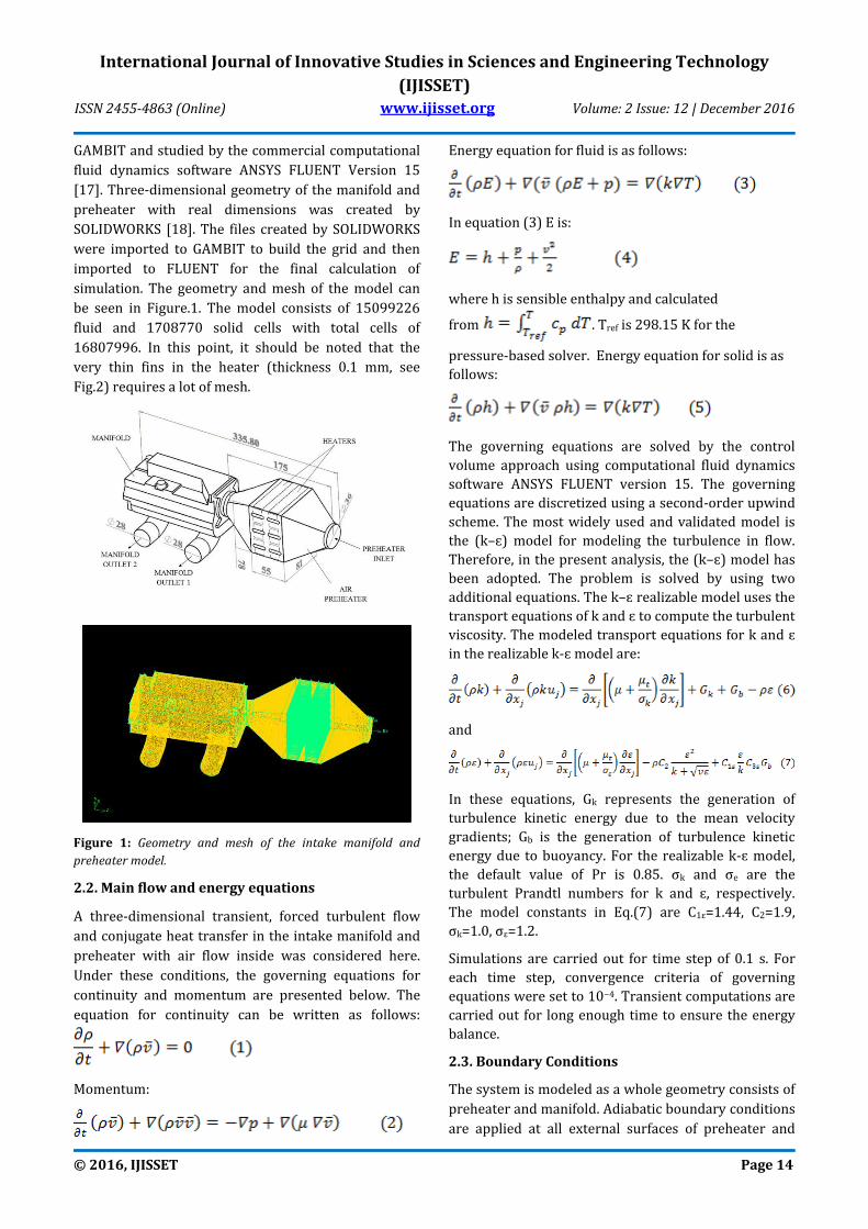
simulation. The geometry and mesh of the model can
be seen in Figure.1. The model consists of 15099226
fluid and 1708770 solid cells with total cells of
16807996. In this point, it should be noted that the
very thin fins in the heater (thickness 0.1 mm, see
Fig.2) requires a lot of mesh.
Figure 1: Geometry and mesh of the intake manifold and
preheater model.
2.2. Main flow and energy equations
A three-dimensional transient, forced turbulent flow
and conjugate heat transfer in the intake manifold and
preheater with air flow inside was considered here.
Under these conditions, the governing equations for
continuity and momentum are presented below. The
equation for continuity can be written as follows:
Momentum:
Energy equation for fluid is as follows:
In equation (3) E is:
where h is sensible enthalpy and calculated
from . Tref is 298.15 K for the
pressure-based solver. Energy equation for solid is as
follows:
The governing equations are solved by the control
volume approach using computational fluid dynamics
software ANSYS FLUENT version 15. The governing
equations are discretized using a second-order upwind
scheme. The most widely used and validated model is
the (k–ɛ) model for modeling the turbulence in flow.
Therefore, in the present analysis, the (k–ɛ) model has
been adopted. The problem is solved by using two
additional equations. The k–ɛ realizable model uses the
transport equations of k and ɛ to compute the turbulent
viscosity. The modeled transport equations for k and ɛ
in the realizable k-ɛ model are:
and
In these equations, Gk represents the generation of
turbulence kinetic energy due to the mean velocity
gradients; Gb is the generation of turbulence kinetic
energy due to buoyancy. For the realizable k-ɛ model,
the default value of Pr is 0.85. σk and σe are the
turbulent Prandtl numbers for k and ɛ, respectively.
The model constants in Eq.(7) are C1ε=1.44, C2=1.9,
σk=1.0, σε=1.2.
Simulations are carried out for time step of 0.1 s. For
each time step, convergence criteria of governing
equations were set to 10−4. Transient computations are
carried out for long enough time to ensure the energy
balance.
2.3. Boundary Conditions
The system is modeled as a whole geometry consists of
preheater and manifold. Adiabatic boundary conditions
are applied at all external surfaces of preheater and
Page 4
International Journal of Innovative Studies in Sciences and Engineering Technology
(IJISSET)
ISSN 2455-4863 (Online) www.ijisset.org Volume: 2 Issue: 12 | December 2016
© 2016, IJISSET Page 15
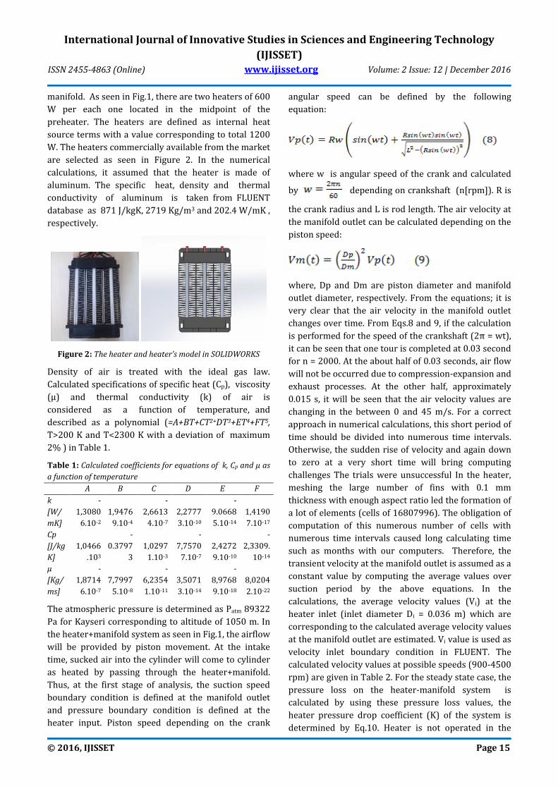
manifold. As seen in Fig.1, there are two heaters of 600
W per each one located in the midpoint of the
preheater. The heaters are defined as internal heat
source terms with a value corresponding to total 1200
W. The heaters commercially available from the market
are selected as seen in Figure 2. In the numerical
calculations, it assumed that the heater is made of
aluminum. The specific heat, density and thermal
conductivity of aluminum is taken from FLUENT
database as 871 J/kgK, 2719 Kg/m3 and 202.4 W/mK ,
respectively.
Figure 2: The heater and heater’s model in SOLIDWORKS
Density of air is treated with the ideal gas law.
Calculated specifications of specific heat (Cp), viscosity
(µ) and thermal conductivity (k) of air is
considered as a function of temperature, and
described as a polynomial (=A+BT+CT2+DT3+ET4+FT5,
T>200 K and T<2300 K with a deviation of maximum
2% ) in Table 1.
Table 1: Calculated coefficients for equations of k, Cp and µ as
a function of temperature
A B C D E F
k
[W/
mK]
-
1,3080
6.10-2
1,9476
9.10-4
-
2,6613
4.10-7
2,2777
3.10-10
-
9.0668
5.10-14
1,4190
7.10-17
Cp
[J/kg
K]
1,0466
.103
-
0.3797
3
1,0297
1.10-3
-
7,7570
7.10-7
2,4272
9.10-10
-
2,3309.
10-14
µ
[Kg/
ms]
-
1,8714
6.10-7
7,7997
5.10-8
-
6,2354
1.10-11
3,5071
3.10-14
-
8,9768
9.10-18
8,0204
2.10-22
The atmospheric pressure is determined as Patm 89322
Pa for Kayseri corresponding to altitude of 1050 m. In
the heater+manifold system as seen in Fig.1, the airflow
will be provided by piston movement. At the intake
time, sucked air into the cylinder will come to cylinder
as heated by passing through the heater+manifold.
Thus, at the first stage of analysis, the suction speed
boundary condition is defined at the manifold outlet
and pressure boundary condition is defined at the
heater input. Piston speed depending on the crank
angular speed can be defined by the following
equation:
where w is angular speed of the crank and calculated
by depending on crankshaft (n[rpm]). R is
the crank radius and L is rod length. The air velocity at
the manifold outlet can be calculated depending on the
piston speed:
where, Dp and Dm are piston diameter and manifold
outlet diameter, respectively. From the equations; it is
very clear that the air velocity in the manifold outlet
changes over time. From Eqs.8 and 9, if the calculation
is performed for the speed of the crankshaft (2π = wt),
it can be seen that one tour is completed at 0.03 second
for n = 2000. At the about half of 0.03 seconds, air flow
will not be occurred due to compression-expansion and
exhaust processes. At the other half, approximately
0.015 s, it will be seen that the air velocity values are
changing in the between 0 and 45 m/s. For a correct
approach in numerical calculations, this short period of
time should be divided into numerous time intervals.
Otherwise, the sudden rise of velocity and again down
to zero at a very short time will bring computing
challenges The trials were unsuccessful In the heater,
meshing the large number of fins with 0.1 mm
thickness with enough aspect ratio led the formation of
a lot of elements (cells of 16807996). The obligation of
computation of this numerous number of cells with
numerous time intervals caused long calculating time
such as months with our computers. Therefore, the
transient velocity at the manifold outlet is assumed as a
constant value by computing the average values over
suction period by the above equations. In the
calculations, the average velocity values (Vi) at the
heater inlet (inlet diameter Di = 0.036 m) which are
corresponding to the calculated average velocity values
at the manifold outlet are estimated. Vi value is used as
velocity inlet boundary condition in FLUENT. The
calculated velocity values at possible speeds (900-4500
rpm) are given in Table 2. For the steady state case, the
pressure loss on the heater-manifold system is
calculated by using these pressure loss values, the
heater pressure drop coefficient (K) of the system is
determined by Eq.10. Heater is not operated in the
Page 5
International Journal of Innovative Studies in Sciences and Engineering Technology
(IJISSET)
ISSN 2455-4863 (Online) www.ijisset.org Volume: 2 Issue: 12 | December 2016
© 2016, IJISSET Page 16
calculations made for the formation of Table 2. These
results will assist in the calculation of the vacuum
pressure in the cylinder.
Table 2: Results of pre-calculations
Vi[m/s] Vm [m/s] Δ P [Pa] K
5 8.3229 112.01 3.234
10 16.629 430.74 3.115
20 33.255 1680.20 3.038
30 49.886 3744 3.009
40 66.512 6628 2.996
50 83.316 10316 2.972
60 99.759 14801 2.974
According to the calculations given in Table 2, it was
seen that there is a significant pressure difference
between inlet and outlet of the system. At the same
time, the pressure loss coefficient is about 3.0 for all
crank cycles
In Table 2, the pressure loss in the preheater and
manifold (ΔP) and heater pressure drop coefficient (K)
is calculated from the following equations for different
velocity inlet values (Vi):
where ρ and Vm is air density and manifold outlet
velocity, respectively.
In the second stage of the calculations, time-dependent
calculations are performed. In these calculations, the
heaters with 1200 W power were run and the air
temperature of manifold outlet has been followed. For
these calculations, velocity inlet boundary condition at
the manifold outlet is applied as negative constant
velocity (corresponding to velocities in Table-2) to
achieve an accurate boundary condition. Thus vacuum
pressure is obtained by applying negative velocity. The
preheater inlet is chosen as pressure inlet at the
atmospheric pressure. The initial temperatures of the
air, heater and manifold are chosen as 258 K and 300 K
for winter and summer design values for Kayseri,
respectively.
3. RESULTS AND DISCUSSION
The numerical calculations are performed for Vm=20,
30, 60 and 90 m/s air flow velocities at the manifold
outlet for a time period of 150 s. Calculations are
realized for both winter and summer conditions. The
initial temperatures of the system and air are assumed
as 258 K and 300 K that Kayseri city are winter and
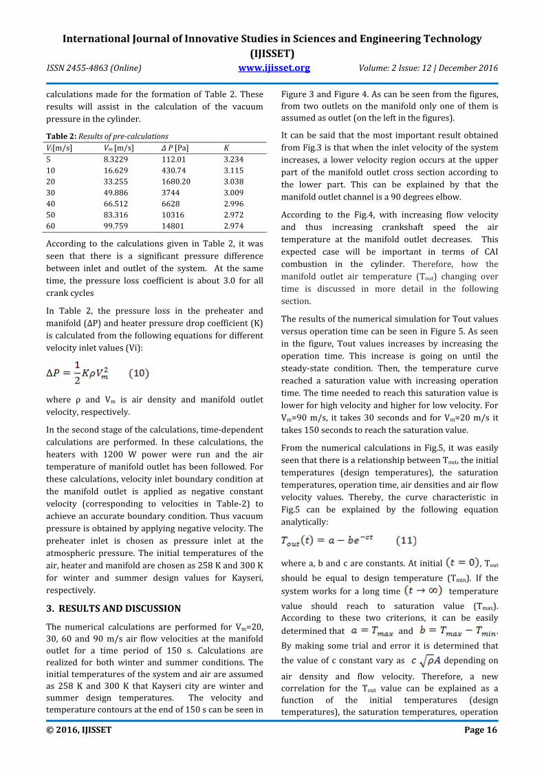
summer design temperatures. The velocity and
temperature contours at the end of 150 s can be seen in
Figure 3 and Figure 4. As can be seen from the figures,
from two outlets on the manifold only one of them is
assumed as outlet (on the left in the figures).
It can be said that the most important result obtained
from Fig.3 is that when the inlet velocity of the system
increases, a lower velocity region occurs at the upper
part of the manifold outlet cross section according to
the lower part. This can be explained by that the
manifold outlet channel is a 90 degrees elbow.
According to the Fig.4, with increasing flow velocity
and thus increasing crankshaft speed the air
temperature at the manifold outlet decreases. This
expected case will be important in terms of CAI
combustion in the cylinder. Therefore, how the
manifold outlet air temperature (Tout) changing over
time is discussed in more detail in the following
section.
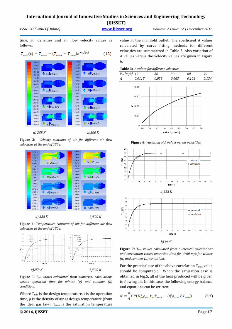
The results of the numerical simulation for Tout values
versus operation time can be seen in Figure 5. As seen
in the figure, Tout values increases by increasing the
operation time. This increase is going on until the
steady-state condition. Then, the temperature curve
reached a saturation value with increasing operation
time. The time needed to reach this saturation value is
lower for high velocity and higher for low velocity. For
Vm=90 m/s, it takes 30 seconds and for Vm=20 m/s it
takes 150 seconds to reach the saturation value.
From the numerical calculations in Fig.5, it was easily
seen that there is a relationship between Tout, the initial
temperatures (design temperatures), the saturation
temperatures, operation time, air densities and air flow
velocity values. Thereby, the curve characteristic in
Fig.5 can be explained by the following equation
analytically:
where a, b and c are constants. At initial , Tout
should be equal to design temperature (Tmin). If the
system works for a long time temperature
value should reach to saturation value (Tmax).
According to these two criterions, it can be easily
determined that and .
By making some trial and error it is determined that
the value of c constant vary as depending on
air density and flow velocity. Therefore, a new
correlation for the Tout value can be explained as a
function of the initial temperatures (design
temperatures), the saturation temperatures, operation
Page 6
International Journal of Innovative Studies in Sciences and Engineering Technology
(IJISSET)
ISSN 2455-4863 (Online) www.ijisset.org Volume: 2 Issue: 12 | December 2016
© 2016, IJISSET Page 17
time, air densities and air flow velocity values as
follows:
a) 258 K b)300 K
Figure 3: Velocity contours of air for different air flow
velocities at the end of 150 s.
a) 258 K b)300 K
Figure 4: Temperature contours of air for different air flow
velocities at the end of 150 s.
a)258 K b)300 K
Figure 5: Tout values calculated from numerical calculations
versus operation time for winter (a) and summer (b)
conditions.
Where Tmin is the design temperature, t is the operation
time, ρ is the density of air at design temperature (from
the ideal gas law), Tmax is the saturation temperature
value at the manifold outlet. The coefficient A values
calculated by curve fitting methods for different
velocities are summarized in Table 3. Also variation of
A values versus the velocity values are given in Figure
6.
Table 3: A values for different velocities
Vm [m/s] 10 20 30 60 90
A 0,0115 0,039 0,063 0,108 0,134
Figure 6: Variation of A values versus velocities.
a)258 K
b)300K
Figure 7: Tout values calculated from numerical calculations
and correlation versus operation time for V=60 m/s for winter
(a) and summer (b) conditions.
For the practical use of the above correlation Tmax value
should be computable. When the saturation case is
obtained in Fig.5, all of the heat produced will be given
to flowing air. In this case, the following energy balance
and equations can be written:
Page 7
International Journal of Innovative Studies in Sciences and Engineering Technology
(IJISSET)
ISSN 2455-4863 (Online) www.ijisset.org Volume: 2 Issue: 12 | December 2016
© 2016, IJISSET Page 18
If the above equations are rearranged and Tmax value is
extracted then the following equation is obtained:
where R is gas constant for air, CP is the specific heat of
air at the design temperature, N is the total heat power
of the heaters.
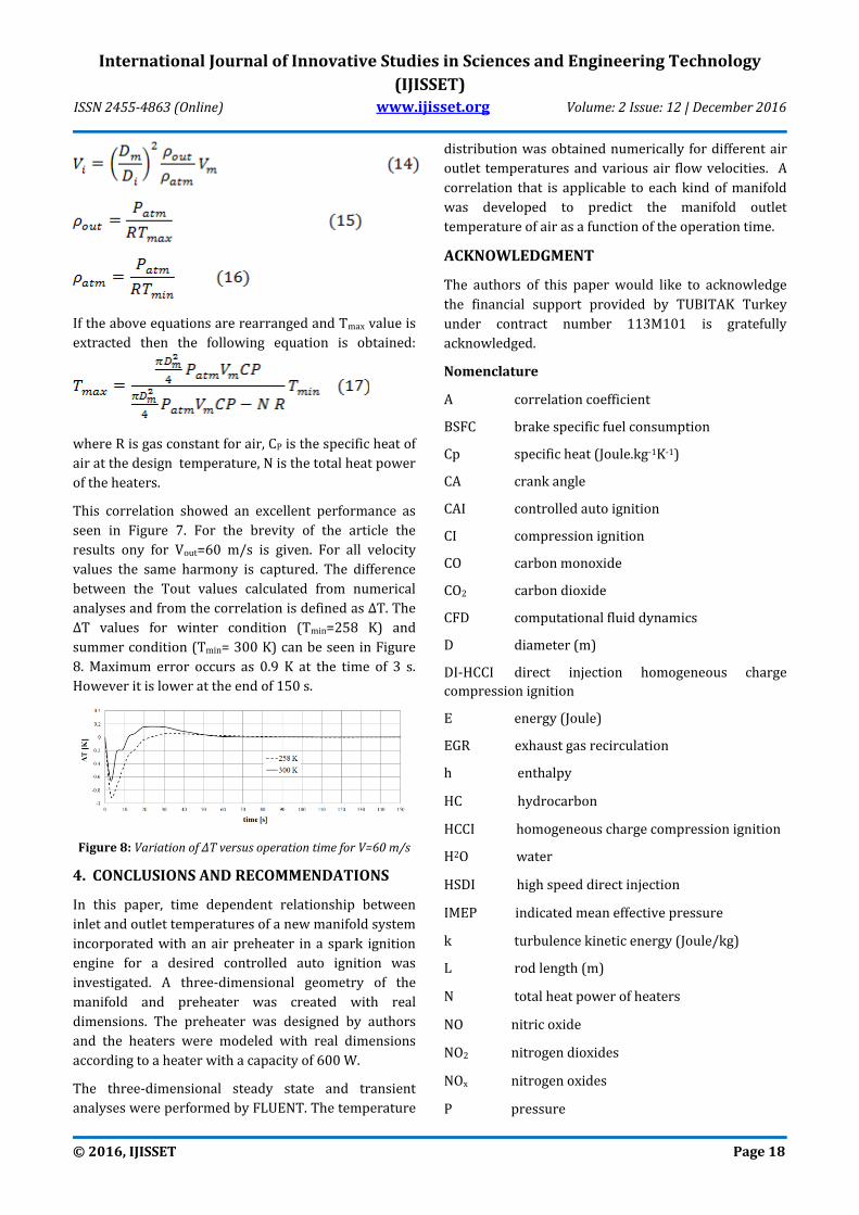
This correlation showed an excellent performance as
seen in Figure 7. For the brevity of the article the
results ony for Vout=60 m/s is given. For all velocity
values the same harmony is captured. The difference
between the Tout values calculated from numerical
analyses and from the correlation is defined as ΔT. The
ΔT values for winter condition (Tmin=258 K) and
summer condition (Tmin= 300 K) can be seen in Figure
8. Maximum error occurs as 0.9 K at the time of 3 s.
However it is lower at the end of 150 s.
Figure 8: Variation of ΔT versus operation time for V=60 m/s
4. CONCLUSIONS AND RECOMMENDATIONS
In this paper, time dependent relationship between
inlet and outlet temperatures of a new manifold system
incorporated with an air preheater in a spark ignition
engine for a desired controlled auto ignition was
investigated. A three-dimensional geometry of the
manifold and preheater was created with real
dimensions. The preheater was designed by authors
and the heaters were modeled with real dimensions
according to a heater with a capacity of 600 W.
The three-dimensional steady state and transient
analyses were performed by FLUENT. The temperature
distribution was obtained numerically for different air
outlet temperatures and various air flow velocities. A
correlation that is applicable to each kind of manifold
was developed to predict the manifold outlet
temperature of air as a function of the operation time.
ACKNOWLEDGMENT
The authors of this paper would like to acknowledge
the financial support provided by TUBITAK Turkey
under contract number 113M101 is gratefully
acknowledged.
Nomenclature
A correlation coefficient
BSFC brake specific fuel consumption
Cp specific heat (Joule.kg-1K-1)
CA crank angle
CAI controlled auto ignition
CI compression ignition
CO carbon monoxide
CO2 carbon dioxide
CFD computational fluid dynamics
D diameter (m)
DI-HCCI direct injection homogeneous charge
compression ignition
E energy (Joule)
EGR exhaust gas recirculation
h enthalpy
HC hydrocarbon
HCCI homogeneous charge compression ignition
H2O water
HSDI high speed direct injection
IMEP indicated mean effective pressure
k turbulence kinetic energy (Joule/kg)
L rod length (m)
N total heat power of heaters
NO nitric oxide
NO2 nitrogen dioxides
NOx nitrogen oxides
P pressure
Page 8
International Journal of Innovative Studies in Sciences and Engineering Technology
(IJISSET)
ISSN 2455-4863 (Online) www.ijisset.org Volume: 2 Issue: 12 | December 2016
© 2016, IJISSET Page 19
R crank radius (m)
rpm revolutions per minute
SI spark ignition
T temperature (K)
t time (s)
V velocity (m/s)
w angular speed (rpm)
ρ density (kg/m3)
ɛ turbulence dissipation rate (Joule kg-1s-1)
µ viscosity (kg m-1 s-1)
REFERENCES
[1] Zhao H, Li J, Ma T, Ladommatos N. Performance
and analysis of a 4-stroke multi-cylinder gasoline
engine with CAI combustion. SAE 2002-01-0420;
2002.
[2] Oakley A, Zhao H, Ladommatos N. Experimental
studies on controlled auto-ignition (CAI)
combustion of gasoline in a 4-stroke engine. SAE
paper 2001-01-1030, 2001.
[3] Kalian N, Zhao H, Qiao J. Investigation of transition
between spark ignition and controlled auto-
ignition combustion in a V6 direct-injection
engine with cam profile switching. J. Automobile
Engineering, 2008;222;1911-26.
[4] Oakley A, Zhao H, Ma T, and Ladommatos N.
Dilution Effects on the Controlled Auto-Ignition
(CAI) Combustion of Hydrocarbon and Alcohol
Fuels, SAE Paper 2001-01-3606.
[5] Broatch A, Luja´n J.M., Serrano J.R., Pla B. A
procedure to reduce pollutant gases from Diesel
combustion during European MVEG-A cycle by
using electrical intake air-heaters. Fuel, 2008: 87;
2760–78.
[6] Payri F, Broatch A, Serrano JR, Rodrı ´guez LF,
Esmorı´s A. Study of the potential of intake air
heating in automotive DI diesel engines. SAE
paper 2006-01-1233; 2006.
[7] Cooper B, Jackson N, Penny I, Rawlins D, Truscott
A, Seabrook J. Advanced combustion system
design, control and optimisation to meet the
requirements of future European passenger cars.
In: THIESEL 2004 conference on thermo-and fluid
dynamic processes in diesel engines; 2004.
[8] Mertz Rolf. Electric intake air heating for small
and medium-sized diesel engines. MTZ
MotortechnischeZeitschrift 1997;58.
[9] Lindl Bruno, Schmitz Heinz-Georg. Cold start
equipment for diesel injection engines. SAE paper
1999-01-1244; 1999.
[10] Gan S., Ng HK, Pang KM. Homogeneous charge
compression ignition (HCCI) combustion:
implementation and effects on pollutants in direct
injection diesel engines. Apply Energy,
2011;88:559–67.
[11] Lü X, Chen W, Huang Z. A fundamental study on
the control of the HCCI combustion and emissions
by fuel design concept combined with controllable
EGR. Part 2.Effect of operating conditions and EGR
on HCCI combustion. Fuel 2005;84:1084–92.
[12] Choi D, Miles PC, Yun H, Reitz RD. A parametric
study of low-temperature, late - injection
combustion in an HSDI diesel engine. JSME Series
B 2005;48(4):656–64.
[13] Jemni M.A., Kantchev G., Abid M.S. Influence of
intake manifold design on in-cylinder flow and
engine performances in a bus diesel engine
converted to LPG gas fuelled, using CFD analyses
and experimental investigations. Energy,
2011:36;2701-15.
[14] Green A.S, Moumtzis T. Case study: use of inlet
manifold design techniques for combustion
applications. Applied Thermal Engineering,
2002:22;1519–27.
[15] Karthikeyan S, Hariganesh R, Sathyanadan M,
Krishnan S, Vadivel P, Vamsidhar D.
Computational analysis of intake manifold design
and experimental investigation on diesel engine
for lcv. International Journal of Engineering
Science and Technology (IJEST), 2011:3;2359-67.
[16] Maftouni N, Ebrahimi R. Intake manifold
optimization by using 3-DCFD analysis with
observing the effect of length of runners on
volumetric efficiency. Proceedings of the 3rd
BSME-ASME International Conference on Thermal
Engineering, 20-22 December, 2006, Dhaka,
Bangladesh.
[17] ANSYS Inc. PDF Documentation for Release 15.0
[18] SolidWorks 2014 Reference Guide by David C.
Planchard