Working Paper 17989http://www.nber.org/papers/w17989
NATIONAL BUREAU OF ECONOMIC RESEARCH1050 Massachusetts Avenue
Cambridge, MA 02138April 2012
We are grateful to seminar participants at the Paris School of Economics, the London School of Economics,the National Bureau of Economic Research (Public Economics Program), the University of Californiaat Berkeley, the Massachussetts Institute of Technology, and Stanford University for their comments.We thank Tony Atkinson, Alan Auerbach, Peter Diamond, Emmanuel Farhi, Mikhail Golosov, LouisKaplow, Wojciech Kopczuk, Matt Weinzierl and Ivan Werning for helpful and stimulating discussions.We acknowledge financial support from the Center for Equitable Growth at UC Berkeley. The viewsexpressed herein are those of the authors and do not necessarily reflect the views of the National Bureauof Economic Research.
NBER working papers are circulated for discussion and comment purposes. They have not been peer-reviewed or been subject to the review by the NBER Board of Directors that accompanies officialNBER publications.
A Theory of Optimal Capital TaxationThomas Piketty and Emmanuel SaezNBER Working Paper No. 17989April 2012JEL No. H21
ABSTRACT
This paper develops a realistic, tractable theoretical model that can be used to investigate socially-optimalcapital taxation. We present a dynamic model of savings and bequests with heterogeneous randomtastes for bequests to children and for wealth per se. We derive formulas for optimal tax rates on capitalizedinheritance expressed in terms of estimable parameters and social preferences. Under our model assumptions,the long-run optimal tax rate increases with the aggregate steady-state flow of inheritances to output,decreases with the elasticity of bequests to the net-of-tax rate, and decreases with the strength of preferencesfor leaving bequests. For realistic parameters of our model, the optimal tax rate on capitalized inheritancewould be as high as 50%-60%–or even higher for top wealth holders–if the social objective is meritocratic(i.e., the social planner puts higher welfare weights on those receiving little inheritance) and if capitalis highly concentrated (as it is in the real world). In contrast to the Atkinson-Stiglitz result, the optimaltax on bequest remains positive in our model even with optimal labor taxation because inequality istwo-dimensional: with inheritances, labor income is no longer the unique determinant of lifetime resources.In contrast to Chamley-Judd, the optimal tax on capital is positive in our model because we have finitelong run elasticities of inheritance to tax rates. Finally, we discuss how adding capital market imperfectionsand uninsurable shocks to rates of return to our optimal tax model leads to shifting one-off inheritancetaxation toward lifetime capital taxation, and can account for the actual structure and mix of inheritanceand capital taxation.
Thomas PikettyParis School of Economics48 Boulevard Jourdan75014 Paris, [email protected]
Emmanuel SaezDepartment of EconomicsUniversity of California, Berkeley530 Evans Hall #3880Berkeley, CA 94720and [email protected]
1 Introduction
According to the profession’s most popular theoretical models, optimal tax rates on capital
should be equal to zero in the long run–including from the viewpoint of those individuals or
dynasties who own no capital at all. Taken literally, the policy implication of those theoretical
results would be to eliminate all inheritance taxes, property taxes, corporate profits taxes,
and individual taxes on capital income and recoup the resulting tax revenue loss with higher
labor income or consumption or lump-sum taxes. Strikingly, even individuals with no capital
or inheritance would benefit from such a change. E.g. according to these models it is in the
interest of propertyless individuals to set property taxes to zero and replace them by poll taxes.
Few economists however seem to endorse such a radical policy agenda. Presumably this
reflects a lack of faith in the standard models and the zero-capital tax results - which are indeed
well known to rely upon strong assumptions.1 As a matter of fact, all advanced economies
impose substantial capital taxes. For example, the European Union currently raises 9% of GDP
in capital taxes (out of a total of 39% of GDP in total tax revenues) and the US raises about
8% of GDP in capital taxes (out of a total of about 27% of GDP in total tax revenues).2
However, in the absence of an alternative tractable model, the zero capital tax result remains
an important reference point in economics teaching and in policy discussions.3 For instance,
a number of economists and policy-makers support tax competition as a way to impose zero
optimal capital taxes to reluctant governments.4 We view the large gap between optimal capital
tax theory and practice as one of the most important failures of modern public economics.
The objective of this paper is to develop a realistic, tractable, and robust theory of socially
optimal capital taxation. By realistic, we mean a theory providing optimal tax conclusions
that are not fully off-the-mark with respect to the real world (i.e., positive and significant
capital tax rates–at least for some parameter values). By realistic, we also mean a theory
offering such conclusions for reasons that are consistent with the reasons that are at play in the
real world which–we feel–are related to the large concentration of inherited capital ownership.
1In particular, Atkinson and Stiglitz (1976; 1980, pp. 442-451) themselves have repeatedly stressed thattheir famous zero capital tax result relies upon unplausibly strong assumptions (most notably the absence ofinheritance and the separability of preferences), and has little relevance for practical policy discussions. See alsoAtkinson and Sandmo (1980) and Stiglitz (1985).
2See European Commission (2011), p.282 (total taxes) and p.336 (capital taxes), for GDP-weighted EU 27averages, and OECD (2011) for the United States.
3Lucas (1990, p.313) celebrates the zero-capital-tax result of Chamley-Judd as “the largest genuinely freelunch I have seen in 25 years in this business.”
4See Cai and Treisman (2005) and Edwards and Mitchell (2008) for references.
1
By tractable, we mean that optimal tax formulas should be expressed in terms of estimable
parameters and should quantify the various trade-offs in a simple and plausible way. By robust,
we mean that our results should not be too sensitive to the exact primitives of the model nor
depend on strong homogeneity assumptions for individual preferences. Ideally, formulas should
be expressed in terms of estimable “sufficient statistics” such as distributional parameters and
behavioral elasticities and hence be robust to changes in the underlying primitives of the model.5
In our view, the two key ingredients for a proper theory of capital taxation are, first, the
large aggregate magnitude and the high concentration of inheritance, and, next, the imperfection
of capital markets. In models with no inheritance (as in the Aktinson-Stiglitz model where all
wealth is due to life-cycle savings or as in Chamley-Judd where life is infinite) or with egalitarian
inheritance (representative agent model), and with perfect capital markets (i.e. if agents can
transfer resources across periods at a fixed and riskless interest rate r), then the logic for the zero
optimal capital taxation result is compelling–as in the standard Atkinson-Stiglitz or Chamley-
Judd models. Hence, our paper proceeds in two steps.
First, we develop a theory of optimal capital taxation with perfect capital markets. We
present a dynamic model of savings and bequests with heterogeneous random tastes for bequests
to children and for wealth accumulation per se. The key feature of our model is that inequality
permanently arises from two dimensions: differences in labor income due to differences in ability,
and differences in inheritances due to differences in parental tastes for bequests and parental
resources. Importantly, top labor earners and top successors are never exactly the same people,
implying a non-degenerate trade-off between the taxation of labor income and the taxation of
capitalized inheritance. In that context, in contrast to the famous Atkinson-Stiglitz result, the
tax system that maximizes social welfare includes positive taxes on bequests even with optimal
labor taxation because, with inheritances, labor income is no longer the unique determinant
of life-time resources. In sum, two-dimensional inequality requires two-dimensional tax policy
tools.
We derive formulas for optimal tax rates τB on capitalized inheritance expressed in terms
of estimable parameters and social preferences. The long run optimal tax rate τB increases
with the aggregate steady-state flow of bequests to output by, decreases with the elasticity of
bequests with respect to the net-of-tax rate eB, and decreases with the strength of preferences
5Such an approach has yielded fruitful results in the analysis of optimal labor income taxation (see Pikettyand Saez, 2012 for a recent survey).
2
for bequests sb0. Under the assumptions of our model, for realistic parameters, the optimal
linear tax rate on capitalized inheritance would be as high as 50%− 60% under a meritocratic
social objective preferences (i.e., those with little inheritance have high welfare weight in the
social objective function). Because real world inherited wealth is highly concentrated–half of
the population receives close to zero bequest, our results are robust to reasonable changes in
the social welfare objective. For example, the optimal tax policy from the viewpoint of those
receiving zero bequest is very close to the welfare optimum for bottom 50% bequest receivers.
Interestingly, the optimal tax rate τB imposed on top wealth holders can be even larger (say,
70%− 80%), especially if bequest flows are large, and if the probability of bottom receivers to
leave a large bequest is small. Therefore our model can generate optimal tax rates as large as the
top bequest tax rates observed in most advanced economies during the past 100 years, especially
in Anglo-Saxon countries from the 1930s to the 1980s (see Figure 1). To our knowledge, this
is the first time that a model of optimal inheritance taxation delivers tractable and estimable
formulas that can be used to analyze such real world tax policies.
Our model also illustrates the importance of perceptions and beliefs systems about wealth
inequality and mobility (i.e. individual most preferred tax rates are very sensitive to expectations
about bequests received and left), and about the magnitude of aggregate bequest flows. When
bequest flows are small, (e.g., 5% of national income, as was the case in Continental Europe
during the 1950s-1970s), then optimal bequest taxes in our model would be moderate. When
they are large (e.g., 15% of national income as in France currently or over 20% as in the 19th
century France), then optimal bequest taxes in our model would be large–so as to reduce the
tax burden falling on labor earners.6
Second, we show that if we introduce capital market imperfections and uninsurable idiosyn-
cratic shocks to rates of return into our setting, then we can study the optimal tax mix between
one-off inheritance taxation and lifetime capital taxation. With perfect and riskless capital mar-
kets, bequest taxes and capital income taxes are equivalent in our framework. However, with
heterogeneous rates of returns, capital income taxation can provide insurance against return
risk more powerfully than inheritance taxation. If the uninsurable uncertainty about future
returns is large, and the moral hazard responses of the rate of return to capital income tax
rates are moderate, the resulting optimal lifetime capital tax rate τK can be very high–typically
6The historical evolution and theoretical determinants of the aggregate bequest flow by were recently studiedby Piketty (2010, 2011). Figures 4-5 summarize his results. We extend his model to study optimal tax policy.
3
higher than the optimal bequest tax rate τB, and labor tax rate τL. This is consistent with
the fact that in modern tax systems the bulk of aggregate capital tax revenues comes from
lifetime capital taxes (rather than from inheritance taxes). It is also interesting to note that
the countries which experienced the highest top inheritance tax rates also applied the largest
tax rates on top incomes, and particularly so on tax capital incomes (see Figures 2-3). To our
knowledge this is the first time that a model of optimal capital taxation can provide a rational
for why these various policy tools can indeed be complementary.
The paper is organized as follows. Section 2 relates our results to the existing literature. Sec-
tion 3 presents our dynamic model and its steady-state properties. Section 4 presents our basic
formula for the optimal tax rate on capitalized inheritance. Section 5 introduces informational
and capital market imperfections to analyze the optimal mix between inheritance taxation and
lifetime capital taxation. Section 6 extends our results in a number of directions, including
population growth, dynamic efficiency, and tax competition. Section 7 offers some concluding
comments. Most proofs and complete details about extensions are gathered in the appendix.
2 Relation to Existing Literature
There are two main results in the literature in support of zero capital income taxation: Atkinson-
Stiglitz and Chamley-Judd. We discuss each in turn and then discuss the more recent literature.
Atkinson-Stiglitz. Atkinson and Stiglitz (1976) show that there is no need to supplement the
optimal non-linear labor income tax with a capital income tax in a life-cycle model if leisure
choice is (weakly) separable from consumption choices and preferences for consumption are
homogeneous. In that model, the only source of lifetime income inequality is labor skill and
hence there is no reason to redistribute from high savers to low savers (i.e. tax capital income)
conditional on labor earnings.7 This key assumption of the Atkinson-Stiglitz model breaks down
in a model with inheritances where inequality in lifetime income comes from both differences in
labor income and differences in inheritances received. In that context and conditional on labor
earnings, a high level of bequests left is a signal of a high level of inheritances received, which
7Saez (2002) shows that this result extends to heterogeneous preferences as long as time preferences areorthogonal to labor skills. If time preferences are correlated with labor skills, then the optimal tax on savingis positive as it is an indirect way to tax ability. Golosov et al. (2011) calibrate a model where higher skillsindividuals have higher saving taste and show that the resulting optimal capital income tax rate depends signif-icantly on the inter-temporal elasticity of substitution but that the implied welfare gains are relatively small inall cases.
4
provides a rationale for taxing bequests. To see this, consider a model with inelastic and uniform
labor income but with differences in inheritances due to parental differences in preferences
for bequests. In such a model, labor income taxation is useless for redistribution but taxing
inheritances generates redistribution. This important point has been made by Cremer, Pestieau,
and Rochet (2003) in a stylized partial equilibrium model with unobservable inherited wealth
where the optimal tax on capital income becomes positive. Our model allows the government
to directly observe (and hence tax) inherited wealth.
Farhi and Werning (2010) consider a model from the perspective of the first generation of
donors who do not start with any inheritance (so that inheritance and labor income inequality
are perfectly correlated). In this context, bequests would actually be subsidized as they would be
untaxed by Aktinson-Stiglitz (ignoring inheritors) and hence would be subsidized when taking
into account inheritors.8 As we shall see, this result is not robust, in the following sense. In
our model, where people both receive and leave bequests, bequest subsidies can also be socially
optimal, but this will arise only for specific–and unrealistic–parameters (e.g. if there is very
little inequality of inheritance or social welfare weights are concentrated on large inheritors).
For plausible parameter values, however, optimal bequest rates will be positive and large.
Chamley-Judd. Chamley (1986) and Judd (1985) show that the optimal capital income tax
would be zero in the long-run. This zero long-run result holds for two reasons.
First, and as originally emphasized by Judd (1985), the zero rate results happens because
social welfare is measured exclusively from the initial period (or dynasty). In that context, a
constant tax rate on capital income creates a tax distortion growing exponentially overtime–
which cannot be optimal (see Judd 1999 for a clear intuitive explanation). Such a welfare
criterion can only make sense in a context with homogeneous discount rates. In the context
of inheritance taxation where each period is a generation and where preferences for bequests
are heterogeneous across the population, this does not seem like a valid social welfare objective
as children of parents with no tastes for bequests would not be counted in the social welfare
function. We will adopt instead a definition of social welfare based on long-run equilibrium
steady-state utility.9 We show in appendix C how the within generation and across generation
8Kaplow (2001) made similar points informally. Farhi and Werning (2010) also extend their model to manyperiods and connect their results to the new dynamic public finance literature (see below).
9In models with dynamic uncertainty, using the initial period social welfare criteria leads to optimal policieswhere inequality grows without bounds (see e.g. Atkeson and Lucas 1992). Obtaining “immiseration” as anoptimal redistributive tax policy is not realistic and can be interpreted as a failure of the initial period socialwelfare criterion. Importantly, Farhi and Werning (2007) show that considering instead the long-run steady-state
5
redistribution problems can be disconnected using public debt so that there is essentially no
loss of generality in focusing on steady state welfare.
Second, even adopting a long-run steady-state utility perspective, the optimal capital income
tax rate is still zero in the standard Chamley-Judd model. This is because the supply side
elasticity of capital with respect to the net-of-tax return is infinite in the standard infinite
horizon dynastic model with constant discount rate.10 The textbook model predicts enormous
responses of aggregate capital accumulation to changes in capital tax rates, which just do not
seem to be there in historical data. Capital-output ratios are relatively stable in the long run,
in spite of large variations in tax rates (see e.g. Piketty, 2010, p.52). Our theory leaves this
key elasticity as a free parameter to be estimated empirically. Our model naturally recovers the
zero capital tax result of Chamley-Judd when the elasticity is infinite.
New Dynamic Public Finance. The recent and fast growing literature on new dynamic
public finance shows that dynamic labor productivity risk leads to non-zero capital income
taxes (see Golosov, Tsyvinski, Werning, 2006 and Kocherlakota 2010 for recent comprehensive
surveys). The underlying logic is the following. When leisure is a normal good, more savings,
ceteris paribus, will tend to reduce work later on. Thus, discouraging savings through capital
income taxation enhances the ability to provide insurance against future poor labor market
possibilities. Quantitatively however, the welfare gains from distorting savings optimally are
very small in general equilibrium (Farhi and Werning, 2011).11 Our model does not include
future earnings uncertainty because individuals care only about the bequests they leave, inde-
pendently of the labor income ability of their children. This simplification is justified in the
case of bequest decisions as empirical analysis shows that bequests respond only very weakly
to children earnings opportunities (see e.g., Wilhelm, 1996). In contrast to the new dynamic
public finance, we find quantitatively large welfare gains from capital taxation in our model.
Hence, our contribution is independent and complementary to the new dynamic public finance.
Methodologically, the new dynamic public finance solves for the fully optimal mechanism
and hence obtains optimal tax systems that can be complex and history dependent, in contrast
to actual practice. We instead limit ourselves to very simple (and more realistic) tax structures.
equilibrium as we do in this paper eliminates the immiseration results.10This follows from the fact that the net-of-tax rate of return needs to be equal to the (modified) discount
rate in steady-state.11Golosov, Troshkin, and Tsyvinski (2011) also calibrate such a model and show that the size of the optimal
implicit capital income tax wedge is quantitatively fairly modest on average (Figure 2, p. 25).
6
This allows us to consider richer heterogeneity in preferences which we believe is important in
the case of bequests.12 Therefore, we also view our methodological approach as complementary
to this literature (Diamond and Saez, 2011 for a longer discussion of this methodological debate).
Capital market imperfections. A number of papers have shown that the optimal tax on
capital income can become positive when capital market imperfections are introduced, even in
models with no inheritance. Typically, the optimal capital income tax is positive because it is
a way to redistribute from those with no credit constraints (the owners of capital) toward those
with credit constraints (non-owners of capital). Aiyagari (1995) and Chamley (2001) make this
point formally in a model with borrowing constrained infinitely lived agents facing labor income
risk. They show that optimal capital income taxation is positive when consumption is positively
correlated with savings13 but do not attempt to compute numerical values for optimal capital
tax rates. Farhi and Werning (2011) (cited above) also propose a quantitative calibration of an
infinite horizon model with borrowing constraints but they find small welfare gains from capital
taxation. In contrast, Conesa, Kitao, and Krueger (2009) calibrate an optimal tax OLG life-
cycle model with uninsurable idiosyncratic labor productivity shocks and borrowing constraints,
and find τK = 36% and τL = 23% in their preferred specification. The main effect seems to be
that capital income tax is an indirect way to tax more the old and to tax less the young, so
as to alleviate their borrowing constraints. While this is an interesting mechanism, we do not
believe that this is the most important explanation for τK > 0. There are other more direct
ways to address the issue of taxing the young vs. the old (e.g. age-varying income taxes; some
policies, e.g. pension schemes, do depend on age).14 In contrast, the theory of capital taxation
offered in the present paper is centered upon the interaction between inheritance and capital
market imperfections.15
Government time-inconsistency and lack of commitment. Yet another way to explain
real-world, positive capital taxes is to assume time inconsistency and lack of commitment.16
Zero capital tax results are always long run results. In the short run, capital is on the table, and
12As mentioned above, Farhi and Werning (2010) do combine inheritance with new dynamic public finance.They consider more general tax structures than we do but impose more structure on preferences.
13This correlation is always positive in the Aiyagari (1995) model with independent and identically distributedlabor income, but Chamley (2001) shows that the correlation can be negative in some cases.
14On age-dependent taxes, see Weinzierl (2011).15Cagetti and DeNardi (2009) provide very interesting simulations of estate taxation in a model with borrowing
constraints and show that shifting part of the labor tax to the estate tax benefits low income workers. They donot try however to derive optimal tax formulas as we do here.
16See e.g. Farhi, Sleet, Werning and Yeltekin (2011) for a recent model along these lines.
7
it is always tempting for short-sighted governments to have τK > 0, even though the optimal
long run τK is equal to 0%. More generally, if governments cannot commit to long run policies,
they will always be tempted to renege on their past commitments and to implement high capital
tax rates, even though this is detrimental to long run welfare.
We doubt that this is the main reason explaining why we observe positive capital taxes in the
real world. Governments and public opinions seem to view positive and substantial inheritance
tax rates (such as those implemented over the past 100 years in advanced economies, see Figure
1 above) as part of a fair and efficient permanent tax system–not as a consequence of short-
sightedness and lack of commitment. Naturally political actors are not always long-sighted but
they often find ways to commit to long run policies, e.g. by appealing to moral principles–such
as equal opportunity and meritocratic values–that apply to all generations and not only to the
current electorate, or by writing down their favored policies in party platforms. Governments
could also find ways to implement the zero-tax long run optimum by delegating capital tax
decisions to an independent authority with a zero-tax mandate (in the same way as the zero-
inflation mandate of independent central banks), or by promoting international tax competition
and bank secrecy laws. In models where positive capital taxes arise solely because of lack of
commitment, such institutional arrangements would indeed be optimal.17
In contrast, we choose in this paper to assume away time inconsistency issues. Hence, we
analyze solely the true long run optimal tax policies–assuming full commitment–and we take
up the most difficult task of explaining positive capital tax rates in such environments.
3 The Model
3.1 Notations and Definitions
We consider a small open economy facing an exogenous, instantaneous rate of return on capital
r ≥ 0. To keep notations minimal, we focus upon a simple model with a discrete set of genera-
tions 0, 1, .., t, .. Each generation has measure one, lives one period (which can be interpreted as
H-year-long, where H = generation length, realistically around 30 years), then dies and is re-
placed by the next generation. Total population is stationary and equal to Nt = 1, so aggregate
variables Yt, Kt,Lt, Bt, and per capita variables yt, kt, lt, bt, are identical (we use the latter).
Generation t receives average inheritance (pre-tax) bt from generation t− 1 at the beginning
17In the real world, believers in zero capital tax policies do support tax competition for this very reason. Seee.g. Edwards and Mitchell (2008). We return to the issue of tax competition in conclusion.
8
of period t. Inheritances go into the capital stock and are invested either domestically or abroad
for a “generational” rate of return 1+R = erH . Production in generation t combines labor from
generation t and capital to produce a single output good. The output produced by generation
t is either consumed by generation t or left as bequest to generation t + 1. We denote by yLt
the average labor income received by generation t. We denote by ct the average consumption of
generation t and bt+1 the average bequest left by generation t to generation t + 1. We assume
that output, labor income, and capital income are realized at the end of period. Consumption
ct and bequest left bt+1 also take place at the end of the period. This condensed timing greatly
simplifies the notations and exposition of the model but is unnecessary for our results.18
With: yti = (1−τB)btierH +(1−τL)yLti = total after-tax lifetime income combining after-tax
capitalized bequest (1− τB)btierH and after-tax labor income (1− τL)yLti
btierH = bti(1 +R) = capitalized bequest received = raw bequest bti + return Rbti
cti = consumption
wti = end-of-life wealth = bt+1i = pre-tax raw bequest left to next generation
bt+1i = (1− τB)bt+1ierH = after-tax capitalized bequest left to next generation
τB ≥ 0 is the tax rate on capitalized bequest, τL ≥ 0 is the tax rate on labor income
Vti is the utility function assumed to be homogeneous of degree one to allow for balanced
growth (and possibly heterogeneous across individuals).
In order to fix ideas, consider the special Cobb-Douglas (or log-log) case:
Vi(c, w, b) = c1−siwswi bsbi (swi ≥ 0, sbi ≥ 0, si = swi + sbi ≤ 1)
This simple form implies that individual i devotes a fraction si of his lifetime resources to end-
of-life wealth, and a fraction 1 − si to consumption. The parameters swi and sbi measure the
tastes for wealth per se and for bequest (more on this below).
In the general case with Vi(c, w, b) homogeneous of degree one, the fraction si of lifetime
resources saved depends on (1 − τB)erH , i.e., the relative price of bequests. Using the first
order condition of the individual Vic = Viw + (1 − τB)erHVib, we can then define sbi = si · (1 −18All results and optimal tax formulas can be extended to a full-fledged, multi-period, continuous-time model
with overlapping generations and life-cycle savings. See section 6 below.
9
τB)erHVib/Vic and swi = si · Viw/Vic. Hence, si, swi, and sbi are functions of (1− τB)erH instead
of being constant as with Cobb-Douglas where income and substitution effects cancel out.
We use a standard wealth accumulation model with exogenous growth. Per capita output in
generation t is given by a constant return to scale production function yt = F (kt, lt), where kt is
the per capita physical (non-human) capital input and lt is the per capita human capital input
(efficient labor supply). Though this is unnecessary for our results, we assume a Cobb-Douglas
production function: yt = kαt l1−αt to simplify the notations .
Per capita human capital lt is the sum over all individuals of raw labor supply lti times
labor productivity hti : lt =∫i∈Nt ltihtidi. Average productivity ht is assumed to grow at some
exogenous rate 1 + G = egH per generation (with g ≥ 0): ht = h0egHt. With inelastic labor
Taking as given the generational rate of return R = erH−1, profit maximization implies that
the domestic capital input kt is chosen so that FK = R, i.e. kt = β1
1−α lt (with β =ktyt
=α
R=
domestic generational capital-output ratio).19 It is important to keep in mind that yt is domestic
output. In the open economy case we consider, yt might differ from national income if the
domestic capital stock kt (used for domestic production) differs from the national wealth bt.
It follows that output yt = βα
1−α lt = βα
1−αh0egHt also grows at rate 1 + G = egH per
generation. So does aggregate labor income yLt = (1 − α)yt. The aggregate economy is on a
steady-state growth path where everything grows at rate 1 +G = egH per generation.
E.g. with g = 1− 2% per year and H = 30 years, 1 +G = egH ' 1.5− 2. With r = 3%− 5%
per year and H = 30 years, 1 +R = erH ' 3− 4.
3.2 Steady-state Inheritance Flows and Distributions
The individual-level transition equation for bequest is the following:
bt+1i = sti · [(1− τL)yLti + (1− τB)btierH ] (1)
In our model, there are three independent factors explaining why different individuals receive
different bequests bt+1i within generation t + 1: their parents received different bequests bti,
earned different labor income yLti, or had different tastes for savings sti = swti + sbti.20
19The annual capital-output ratio is βa = H · β = α(H/R) = αH/(erH − 1) ' α/r if r is small.20A fourth important factor in the real world is the existence of idiosyncratic shocks to rates of return rti
(see section 5). Pure demographic shocks (such as shocks to the age at parenthood, age at death of parents andchildren, number of children, rank of birth, etc.) also play an important role.
10
Savings Tastes. Importantly, taste parameters vary across individuals and over time in our
model. E.g. some individuals might have zero taste for wealth and bequest (swti = sbti = 0), in
which case they save solely for life-cycle purposes and die with zero wealth (“life-cycle savers”).
Others might have taste for wealth but not for bequest (swti > 0, sbti = 0) (“wealth-lovers”),
while others might have no direct taste for wealth but taste for bequest (swti = 0, sbti > 0)
(“bequest-lovers”). The taste for wealth could reflect direct utility for the prestige or social
status conferred by wealth. In presence of uninsurable productivity shocks, it could also measure
the security brought by wealth, i.e. its insurance value (so this modeling can be viewed as a
reduced form for precautionary saving). The only difference between wealth- and bequest-lovers
is that the former do not care about bequest taxes while the latter do.
In the real world, most individuals are at the same time life-cycle savers, wealth-lovers
and bequest-lovers. But the exact magnitude of these various saving motives does vary a lot
across individuals and over generations, just like other tastes.21 We allow for any exogenous
distribution for taste parameters g(swi, sbi). For notational simplicity, we assume that tastes are
drawn i.i.d. at each generation from the distribution g(swi, sbi). Hence they are independent
across individuals within a generation and independent across generations within a dynasty. In
the Cobb-Douglas case, the parameters swi, sbi are fixed independently of τB. In the general
homogeneous of degree one case, the parameters swi, sbi depend upon (1− τB)erH and hence are
not strictly parameters. We adopt this slight abuse of notation for presentational simplicity.22
Assumption 1 Taste parameters (swi, sbi) are drawn i.i.d. at each generation from an exoge-
nous distribution g(swi, sbi) defined over a set of possible tastes S ⊂ S (where S is the set of all
possible tastes: S = {(swi, sbi) s.t. swi, sbi ≥ 0 and si = swi + sbi ≤ 1}).
S and g(·) can be discrete or continuous. We denote by s0 = min {si = swi + sbi ∈ S}, s1
= max {si = swi + sbi ∈ S}, with 0 ≤ s0 ≤ s1 ≤ 1, and s = E(si) the average taste.
We assume that S includes zero saving tastes and at least one other taste: s0 = 0, s1 > 0.
Assumption 1 implies that in each generation there are “zero bequest receivers” (i.e. individ-
uals who receive zero bequest, because their parents had zero taste for wealth and bequest).23
Productivity Shocks. Labor productivity shocks are specified as follows. Individual i in
generation t has a within-cohort normalized productivity parameter θti = hti/ht. By definition,
21Kopczuk and Lupton (2007) and Kopczuk (2009, 2012) present evidence on heterogeneity in bequest motives.22Rigorously, we would need to parametrize utility functions so that sbi = sb(σbi, (1 − τB)erH), swi =
sw(σwi, (1− τB)erH) with (σbi, σwi) i.i.d parameters and sb(.) and sw(.) fixed functions.23This could result from other types of shocks (see example below).
11
we have: yLti = θtiyLt (with E(θti) = 1). Productivity differentials θti could come from innate
abilities, acquired skills, individual occupational choices, or sheer luck–and most likely from a
complex combination between the four. We assume that productivity shocks are drawn i.i.d.
from the same distribution h(θi) at each generation and independently of savings tastes.
Assumption 2 Productivity parameters θi are drawn i.i.d. at each generation from an exoge-
nous distribution h(θi) over some productivity set Θ ⊂ [0,+∞[ independently of savings tastes.
The set Θ and the distribution h(·) can be discrete or continuous. We note: θ0 = min {θi ∈ Θ}
and θ1 = max {θi ∈ Θ}, with 0 ≤ θ0 ≤ 1 ≤ θ1 ≤ +∞. By construction: E(θi) = 1.
All our results can readily be extended to a setting with some intergenerational persistence
of savings tastes and productivities. In that case, to ensure the existence of a unique ergodic
steady-state joint distribution of inherited wealth and productivities, one would simply need to
assume that the random process for tastes satisfies a simple ergodicity property. Any individual
has a positive probability of having any savings taste×productivity no matter what his or her
parental savings taste×productivity were (see appendix A1).
Steady State Distributions. Under assumptions 1-2, the individual transition equation (1)
can be aggregated into:
bt+1 = s · [(1− τL)yLt + (1− τB)bterH ] (2)
Let us denote the aggregate capitalized bequest flow-domestic output ratio by byt =erHbtyt
.
Dividing both sides of equation (2) by per capita domestic output yt and noting that bt+1/yt =
byt+1e−(r−g)H , we obtain the following transition equation for byt:
To ensure convergence towards a non-explosive steady-state, we must assume that the average
taste for wealth and bequest is not too strong:
Assumption 3 s · e(r−g)H < 1
If assumption 3 is violated, the economy can accumulate infinite wealth relative to domestic
output, and will cease to be a small open economy at some point so that the world rate of
return will have to fall to restore assumption 3. If assumption 3 is satisfied, then, as τB ≥ 0,
byt → by =s(1− τL)(1− α)e(r−g)H
1− s(1− τB)e(r−g)H as t → +∞. I.e. the aggregate inheritance-output ratio
converges towards a finite value, and in steady-state, bequests grow at the same rate as output.
12
Finally, we denote by zti = bti/bt the within-cohort normalized bequest, and φt(z) the
distribution of normalized bequest within cohort t. Given some initial distribution φ0(z), the
random processes for tastes and productivity g(·) and h(·) and the individual transition equation
(1) entirely determine the low of motion for the distribution of inheritance φt(z) and the joint
distribution of inheritance and labor productivity, which we denote by ψt(z, θ) = φt(z) · h(θ).
Proposition 1 (a) Under assumptions 1-3, there is a unique steady-state for the aggregate in-
heritance flow-output ratio by, the inheritance distribution φ(z), the joint inheritance-productivity
distribution ψ(z, θ). For any initial conditions, as t→∞, byt → by, φt(·)→ φ and ψt → ψ.
(b) We have: by =s(1− τL)(1− α)e(r−g)H
1− s(1− τB)e(r−g)H .
(c) The joint inheritance-productivity distribution ψ(z, θ) = φ(z) · h(θ) is two-dimensional.
At any productivity level, the distribution involves zero-bequest receivers and is non-degenerate.
I.e. z0 = min {z s.t. φ(z) > 0} = 0 < z1 = max {z s.t. φ(z) > 0} ≤ ∞
Proof. The result follows from standard ergodic convergence theorems (Appendix A1). QED
Two points are worth noting. First, the aggregate magnitude of inheritance flows relative
to output by grows with r − g. With high returns and low growth, wealth coming from the
past is being capitalized at a faster rate than national income. Successors simply need to save
a small fraction of their asset returns to ensure that their inherited wealth grows at least as
fast as output. The multiplicative factor associated to intergenerational wealth transmission
is large and leads to high inheritance flows. Conversely, with low returns and high growth,
inheritance is dominated by new wealth, and the steady-state aggregate inheritance flow is
a small fraction of output. As shown in Piketty (2011), this simple r-vs-g model is able to
reproduce remarkably well the observed evolution of aggregate inheritance flows over the past
two centuries. In particular, it can explain why inheritance flows were so large in the 19th and
early 20th centuries (20%-25% of national income in 1820-1910), so low in the mid-20th century
(less than 5% around 1950-1960), and why they are becoming large again in the late 20th and
early 21st centuries (about 15% in 2010 in France) (see Figures 4-5). With r = 4% − 5% and
g = 1%− 2%, simple calibrations of the above formula show that the annual inheritance flow by
can indeed be as large as 20%− 25% of national income.24 Available evidence suggests that the
24E.g. with r − g = 3%, H = 30, α = 30%, s = 10%, τB = τL = 0%, then by = 23%. With r − g = 2%,then by = 16%. With r − g = 3% and τ = 30%, then by = 13%, but by/(1 − τ) = 19%. The by formula givenabove relates to the generational, (capitalized bequest)/output ratio, while the empirical estimates depictedon Figures 4-5 refer to the cross-sectional, non-capitalized ratio. But one can show that both ratios are very
13
French pattern also applies to Continental European countries that were hit by similar growth
and capital shocks. The long-run U-shaped pattern of aggregate inheritance flows was possibly
somewhat less pronounced in the United States or United Kingdom (Piketty, 2010, 2011).
Second, one important feature of our model–and of the real world–is that inequality is two-
dimensional. In steady-state, the relative positions in the distributions of inheritance and labor
productivity are never perfectly correlated. This is the key property that we need for our
optimal tax problem to make sense and for our results to hold: Labor income is not a perfect
predictor for inheritance. With i.i.d. taste and productivity shocks, we even get that the two
distributions are independent (ψ(z, θ) = φ(z) · h(θ)). All our results would still hold if we
introduce some intergenerational persistence of tastes and productivities, as long as persistence
is not complete and the two dimensions of shocks are not perfectly correlated. As we shall see
below, this two-dimensionality property is the key feature explaining why the Atkinson-Stiglitz
result does not hold in our model, and why we need a two-dimensional tax policy tool (τB, τL).
3.3 An Example with Binomial Random Tastes
A simple example might be useful in order to better understand the logic of two-dimensional
inequality and the role played by random tastes in our model. Assume that taste shocks take only
two values: si = s0 = 0 with probability 1−p, and si = s1 > 0 with probability p. The aggregate
saving rate is equal to s = E(si) = ps1. Let µ = s(1− τB)e(r−g)H , µ1 = s1(1− τB)e(r−g)H = µ/p.
Assume µ < 1 < µ/p, and no productivity heterogeneity: Θ = {1}. One can easily show that
the steady-state inheritance distribution φ(z) is discrete and looks as follows:
z = z0 = 0 with probability 1− p (children with zero-wealth-taste parents).
z = z1 =1− µp
> 0 with probability (1 − p) · p (children with wealth-loving parents but
zero-wealth-taste grand-parents).
...
z = zk =1− µp
+µ
p· zk−1 =
1− µµ− p
·
[(µ
p
)k− 1
]with probability (1− p) · pk+1 (children with
wealth-loving ancestors during the past k+1 generations, but zero-wealth-taste k+2-ancestors).
That is, the steady-state distribution φ(z) is unbounded above and has the standard Pareto
asymptotic upper tail found in empirical data and in wealth accumulation models with random
multiplicative shocks (see Appendix A1 and Atkinson, Piketty and Saez (2011)). Inheritances
close when inheritance tends to happen around mid-life (see section 6 below). Piketty (2010, 2011) presentsdetailed simulations using a full-fledged, out-of-steady-state version of this model, with life-cycle savings and fulldemographic and macroeconomic shocks.
14
are obviously uncorrelated with labor income (since there is no inequality of labor income).
Taste shocks could also be interpreted as shocks to rates of return (e.g., p is the probability
that one gets a high return, and 1−p is the probability that one goes bankrupt, thereby leaving
zero estate) or as a demographic shocks (e.g., p is the probability that one dies at a “normal
age” and with “normal” health costs, and 1 − p is the probability that one dies very old or
after large health costs, thereby leaving zero estate; shocks on number of children or rank of
birth could also do). As long as the shocks have a multiplicative structure, the steady-state
distribution of inheritance will have a Pareto upper tail, with a Pareto coefficient reflecting
the relative importance of the various effects (see Appendix A1). In practice all these types
of shocks clearly exist and matter a lot. The key point is that there are many factors - other
than productivity shocks - explaining the large inequality of inherited wealth that we observe
in the real world. The main limitation of models of wealth accumulation based solely upon
productivity shocks is that they massively under-predict wealth concentration.25
If we introduce productivity shocks (say θti = θ0 ≥ 0 with probability 1 − q and θti =
θ1 > 1 > θ0 with probability q), the steady-state joint distribution ψ(z, θ) is simply the product
of the two distributions, i.e. ψ(z, θ) = φ(z) · h(θ). So the joint distribution again involves
zero correlation between the two dimensions. If we further introduce some intergenerational
persistence in the productivity process (say, θt+1i = θ1 with probability q0 if θti = θ0, and
with probability q1 ≥ q0 if θti = θ1), then the steady-state distribution ψ(z, θ) will involve
some positive correlation between the two dimensions. But the correlation will always be less
than one: the entire history of ancestors’ tastes sti, st−1i, etc. and productivity shocks θti, θt−1i,
etc. matters for the determination of the current inheritance position zt+1i, while only parental
productivity θti matters for the current productivity position θt+1i.26
3.4 The Optimal Tax Problem
We now formally define our optimal tax problem. We assume that the government faces an
exogenous revenue requirement: per capita public good spending must satisfy gt = τyt where
τ ≥ 0 is taken as given and yt is exogenous per capita domestic output. We first assume
that the government has only two tax instruments: a proportional tax on labor income at rate
τL ≥ 0, and a proportional tax on capitalized inheritance at rate τB ≥ 0. We impose a period-
25See discussion on homogeneous tastes in Section 6 below and references given in Piketty (2011, section II.C).26Our results can also be extended to a model without random tastes, as long as productivity shocks include
a zero lower bound (see Section 6).
15
by-period (i.e. generation-by-generation) budget constraint: the government must raise from
labor income yLt and capitalized inheritance bterH received by generation t an amount sufficient
to cover government spending τyt for generation t.27 We again assume that everything takes
place at the end of period: output is realized, taxes are paid, government spending and private
consumption occur. Hence, the period t government budget constraint looks as follows:
We assume that τ < 1−α, i.e. the public good spending requirement is not too large and could
be covered by a labor tax alone (in case the government so wishes).
Assumption 4 τ < 1− α
It is worth stressing that all taxes are paid at the end of the period, and that the tax τB
is a tax on capitalized bequest bterH = bt(1 + R), not a tax on raw bequest bt. One natural
interpretation of this tax on capitalized bequest is that at the end of the period the government
taxes both raw bequests bt and capital income (returns to bequest) Rbt at the same rate τB. So
the tax τB should really be viewed as a broad based “capital tax” (falling on wealth transmission
as well as as on the returns to wealth) rather than a narrow based bequest tax. Note that as
long as capital markets are perfect and everybody gets the same rate of return (we relax this
assumption in section 5 below), it really does not matter how the government chooses to split
the capital tax burden between one-off inheritance taxation and lifetime capital taxation on the
flow return. In particular, rather than taxing bequests bt and the returns to bequest Rbt at the
same rate τB, it would also be equivalent not to tax bequest bt and instead to have a larger,
single tax on the returns to capital Rbt at rate τK such that:28
(1− τB)(1 +R) = 1 + (1− τK)R i.e. τK =τB(1 +R)
R=
τBerH
erH − 1
Example. Assume r = 4%, H = 30, so that erH = 1 +R = 3.32, i.e. R = 2.32.
If τB = 20% then τK = 29%. If τB = 40% then τK = 57%. If τB = 60% then τK = 86%.
27We introduce intergenerational redistribution in Section 6 (appendix C provides complete details).28Here it is critical to assume that the utility function Vti = V (cti, wti, bt+1i) is defined over after-tax capitalized
bequest bt+1i = [1 − τB + (1 − τK)R]bt+1i. If Vti were defined over after-tax non-capitalized bequest bt+1i =(1− τB)bt+1i, then zero-receivers would strictly prefer capital income taxes over bequest taxes (in effect τK > 0would allow them to tax positive receivers without reducing their utility from giving a bequest to their ownchildren). However this would amount to tax illusion, so we rule this out.
16
Hence, it is equivalent to tax capitalized bequests at τB = 40% or to tax capital income
flows at τK = 57% (or τK = 43% if the we take the equivalent instantaneous tax rate).29 More
generally, any intermediate combination will do. I.e. for any tax mix (τB, τK), τB is a tax on raw
bequest and τK is an extra tax on the return to bequest, one can define τB = τB + τKR
1 +R.30
Intuitively, τB is the adjusted total tax rate on capitalized bequest. For now, we focus on the
broad capital tax interpretation (τB = τB, i.e. no extra tax on return: τK = 0). In section 5 we
introduce capital market imperfections to analyze the optimal tax mix between τB and τK .
The question that we now ask is the following: what is the tax policy (τL, τB) maximizing
long-run, steady-state social welfare? That is, we assume that the government can commit
for ever to a tax policy (τLt = τL, τBt = τB)t≥0 and cares only about the long-run steady-
state distribution of welfare Vti. Under assumptions 1-4, for any tax policy there exists a unique
steady-state ratio by and distribution ψ(z, θ). The government chooses (τL, τB) so as to maximize
the following, steady-state social welfare function:31
SWF =
∫∫z≥0,θ≥0
ωpzpθV 1−Γzθ
1− Γdzdθ (5)
With: Vzθ = E(Vi | zi = z, θi = θ) = average steady-state utility level Vi attained by individuals
i with normalized inheritance zi = z and productivity θi = θ.
ωpzpθ = social welfare weights as a function of the percentile ranks pz, pθ in the steady-state
distribution of normalized inheritance z and productivity θ.32
Γ = concavity of the social welfare function (Γ ≥ 0).33
A key parameter to answer this question is the long-run elasticity eB of aggregate inheritance
ratio by with respect to the net-of-bequest-tax rate 1 − τB (letting τL adjust to keep budget
29In the above equation we model the capital income tax τK as taxing the full generational returnRbt all at onceat the end of the period. Alternatively one could define τK as the equivalent annual capital income tax rate during
the H-year period, in which case the equivalence equation would be: 1 − τB = e−τKrH , i.e. τK = − log(1−τB)rH .
Both formulas perfectly coincide for small tax rates and small returns, but differ otherwise. E.g. in the aboveexample, we would have annual τK = 19%, 43%, 76% (instead of generational τK = 29%, 57%, 86%). Note that itwould also be equivalent to have an annual wealth tax or property tax at rate τW = rτK (with a fixed, exogenousrate of return, annual taxes on capital income flows and capital stocks are equivalent).
30The tax on raw bequest τBbt is paid at the end of the period, and the tax payment is assumed to beτBbt(1 +R), so in effect τK can be interpreted as an extra tax on the return to bequest.
31This steady-state maximization problem can also be formulated as the asymptotic solution of an inter-temporal social welfare maximization problem. See Appendix C, Proposition C1.
32Here we implicitly assume that the welfare weights ωi are the same for all individuals i with the same rankspz, pθ in the distribution of normalized inheritance and productivity. Our optimal tax formulas can easily beextended to the general case where social welfare weights ωi also depend upon taste parameters swi and sbi -which can be justified for utility normalization purposes. See the discussion in Appendix A2.
33If Γ = 1, then SWF =∫∫z≥0,θ≥0
ωpzpθ log(Vzθ)dΨ(z, θ).
17
balance, see equation (4)):
eB =1− τBby
dbyd(1− τB)
(6)
In general, one might expect eB > 0: with a higher net-of-tax rate 1− τB, agents may choose to
devote a larger fraction of their resources to inheritance, in which case the aggregate, steady-
state inheritance ratio will be bigger. But this could also go the other way, because eB is defined
along a budget balanced steady-state frontier: lower bequest taxes imply higher labor taxes,
which in turn make it more difficult for high labor earners to accumulate large bequests.
Substituting τL(1− α) = τ − τBby into the steady-state formula for by, we obtain:
by =s(1− α− τ)e(r−g)H
1− se(r−g)H (7)
Recall that s does not depend on τB in the Cobb-Douglas case with i.i.d shocks. Therefore,
by depends on τ but not on the tax mix τL, τB and eB = 0 in that case. For general utility
functions and/or random processes, s depends on τB and eB could really take any value (> 0 or
< 0). We view eB as a free parameter to be estimated empirically. There is no reason to expect
eB to be infinitely large, unlike in the infinite-horizon dynastic model of Chamley-Judd.
4 Basic Optimal Capital Tax Formula
4.1 The Zero-Bequest-Receiver Social Optimum
Throughout this paper we are particularly interested in the zero-bequest-receiver social opti-
mum, i.e. the optimal tax policy from the viewpoint of those who receive zero bequest, and
who must rely entirely on their labor income. This corresponds to the case with a linear social
welfare function (Γ = 0) and the following welfare weights: ωpzpθ = 1 if pz = 0 (i.e. z = 0)
and ωpzpθ = 0 if pz > 0. Since the Vi() are homogenous of degree one, Γ = 0 implies that the
government does not want to redistribute income from high productivity to low productivity
individuals–perhaps because individuals are viewed as (partly) responsible for their productiv-
ity parameter θ. In contrast, individuals cannot be responsible for their bequest parameter z.
Therefore trying to reduce as much as possible the inequality of lifetime welfare opportunities
along the inheritance dimension seems normatively appealing.34 So we start by characterizing
this zero-bequest-receiver optimum, which we call the “meritocratic Rawlsian optimum”:
34Perhaps surprisingly, the normative literature on equal opportunity and responsibility has devoted littleattention to the issue of inheritance taxation. E.g. Roemer et al. (2003) and Fleurbaey and Maniquet (2006)focus on labor income taxation. See however the interesting discussion in Fleurbaey (2008, pp.146-148).
18
Proposition 2 (zero-bequest-receiver optimum). Under assumptions 1-4, linear social
welfare (Γ = 0), and the welfare weights: ωpzpθ = 1 if pz = 0, and ωpzpθ = 0 if pz > 0, then:
τB =1− (1− α− τ)sb0/by
1 + eB + sb0and τL =
τ − τBby1− α
with sb0 = E(sbi | zi = 0) = average bequest taste of zero bequest receivers (weighted by marginal
utility×labor income).
Proof. Take a given tax policy (τL, τB). Consider a small increase in the bequest tax rate
dτB > 0. Differentiating the government budget constraint, τL(1−α)+τBby = τ , in steady-state
dτB > 0 allows the government to cut the labor tax rate by:
dτL = −bydτB1− α
(1− eBτB
1− τB
)(< 0 as long as τB <
1
1 + eB)
Note that dτL is proportional to the aggregate inheritance-output ratio by. With a larger
inheritance flow, a given increase in the bequest tax rate can finance a larger labor tax cut.
An individual i who receives no inheritance (bti = 0) chooses bt+1i to maximize
The first order condition in bt+1i is Vci = Vwi + (1 − τB)(1 + R)Vbi This leads to bt+1i =
si(1− τL)yLti (with 0 ≤ si ≤ 1). Recall that sbi = si · (1− τB)(1 +R)Vbi/Vci.35
Using the envelope theorem as bt+1i maximizes utility, the utility change dVi created by a
budget balance tax reform dτB, dτL can be written as follows:
dVi = −VciyLtidτL − Vbi(1 +R)bt+1idτB
I.e.: dVi = VciθiyLtdτB
[(1− eBτB
1− τB
)by
1− α− 1− τL
1− τBsbi
]The first term in the square brackets is the utility gain due to the reduction in the labor
income tax (proportional to by as noted above), while the second term is the utility loss due to
reduced net-of-tax bequest left (naturally proportional to the bequest taste sbi).
By using the fact that 1 − τL = (1 − α − τ + τBby)/(1 − α) (from the government budget
constraint), this can be re-arranged into:
dVi = VciθiyLtdτB1− τL1− τB
[1− (1 + eB)τB
1− α− τ + τBbyby − sbi
].
35In the Cobb-Douglas utility case, sbi is simply the fixed exponent in the utility function. In the generalhomogeneous utility case, sbi may depend on τB and 1 +R.
19
Summing up over all zero-bequest-receivers, we get:
dSWF ∼ dτB
[1− (1 + eB)τB
1− α− τ + τBbyby − sb0
]with sb0 =
E(Vciθisbi | zi = 0)
E(Vciθi | zi = 0).
Setting dSWF = 0, we get the formula: τB =1− (1− α− τ)sb0/by
1 + eB + sb0. QED.
Note 1. This proof works with any utility function that is homogenous of degree one (and not
only in the Cobb-Douglas case) and with any ergodic random process for taste and productivity
shocks (and not only with i.i.d. shocks). In the case with Cobb-Douglas utility functions, the
proof can be further simplified. See Appendix A2.
Note 2. In the general case, sb0 is the average of bequest tastes sbi over all zero-bequest-
receivers, weighted by the product of their marginal utility Vci and of their productivity θi. In
case sbi⊥Vciθi, then sb0 is the simple average of sbi over all zero-bequest-receivers: sb0 = E(sbi |
zi = 0). In the case with i.i.d. shocks and adequate utility normalization, then sb0 is the same
as the average bequest taste for the entire population: sb0 = sb = E(sbi). See Appendix A2.
Note 3. We also show in the appendix how to extend the optimal tax formula to the case
Γ > 0. One simply needs to replace sb0 by: sb0 =E(VciθiV
−Γi sbi | zi = 0)
E(VciθiV−Γi | zi = 0)
. I.e. the formula for
sb0 needs to be reweighted in order to take into account the lower marginal social utility V −Γi
of zero-receivers with high utility Vi (i.e. zero-receivers with high productivity θi).
When the social welfare function is infinitely concave (Γ→ +∞), in effect the planner puts
infinite weight on the least productive, zero-bequest receivers. This is equivalent to assuming
welfare weights ωpzpθ = 1 iff pz = 0 and pθ = 0. Therefore sb0 is simply the average bequest taste
within this group: sb0 = E(sbi | zi = 0, θi = θ0). This could be called the “radical Rawlsian
optimum”. This might be too radical, however, because individuals are - partly - responsible
for their productivity, e.g. through their choice of occupation. From an ethical perspective,
the most appealing social welfare optimum probably lies in between the meritocratic and the
radical Rawlsian optima, depending on how much one considers individuals are responsible for
their productivity (i.e. how much productivity parameters reflect individual choices rather than
innate abilities or sheer luck) - an issue which we do not model explicitly in the present paper.36
Note 4. Using formula (7) for by, we also have τB =1 + sb0 − (sb0/s)e
−(r−g)H
1 + sb0 + eB. This alternative
formula shows more directly how the optimal rate varies with primitives s, sb0, r− g but is more
difficult to calibrate than our formula in Proposition 2 (since we typically have data on by).
36See Piketty and Saez (2012) for a more elaborate normative discussion.
20
4.2 Numerical calibrations
The optimal tax formula τB =1− (1− α− τ)sb0/by
1 + eB + sb0is simple, intuitive, and can easily be
calibrated using empirical estimates.
The optimal tax rate τB decreases with the elasticity of bequests to the net-of-tax rate eB,
increases with the aggregate steady-state flow of inheritances to output by, and decreases with
the strength of preferences for leaving bequests sb0. A higher bequest elasticity eB unsurprisingly
implies a lower τB. As eB → +∞, τB → 0%. I.e. one would never tax an infinitely elastic tax
base as in the dynastic model of Chamley-Judd.
More interestingly, a higher bequest flow ratio by implies a higher τB. This is a very large
That is, with high bequest flow by = 20%, zero receivers want to tax inherited wealth
at a higher rate than labor income (73% vs. 22%); with low bequest flow by = 5%, they
want the opposite (18% vs. 42%). The intuition is the following. In societies with low by
(typically because of high g), there is not much tax revenue to gain from taxing bequests. So
even zero-receivers do not like bequest taxes too much: it hurts their children without bringing
much benefit in exchange. High growth societies care about the future, not about the past.
Conversely, in societies with high by (typically because of low g), it is worth taxing bequests, so
as to reduce labor taxation and improve the welfare of those receiving no inheritance.
In our theory there is really no general reason why capitalized inheritance would be taxed
more or less than labor income. Any situation can be optimal, depending on parameters. With
the low by ratios observed in the 1950s-1960s, it is probably optimal to tax inheritance less than
labor. But with the high by ratios observed in the 1900s-1910s or the 2000s-2010s, it is probably
optimal to tax inheritance more than labor (see Figures 4-5).
It is worth noting that the impact of by is quantitatively more important than the impact of
eB. That is, behavioral responses matter but not hugely as long as the elasticity is reasonable.
Example 2.Assume τ = 30%, α = 30%, sb0 = 10%, by = 15%.
21
If eB = 0, then τB = 67% and τL = 29%.
If eB = 0.2, then τB = 56% and τL = 31%.
If eB = 0.5, then τB = 46% and τL = 33%.
If eB = 1, then τB = 35% and τL = 35%.
This is probably the most important lesson of this paper: once one allows the elasticity of
capital supply to be a free parameter and to take moderate (non-infinite) values, then one can
naturally obtain fairly large levels for socially optimal capital tax rates. That is, if we take
by = 15% (current French level), then we find that as long as the elasticity eB is less than one
the optimal inheritance tax rate is higher than the optimal labor tax rate. With a realistic value
eB = 0.2, we find τB = 56% and τL = 31%.37 In practice, this bequest elasticity effect eB is
also mitigated by the existence of a positive labor supply elasticity effect eL , which makes low
labor taxation and therefore high bequest taxation even more valuable (see section 6).
Finally, a higher bequest taste sb0 implies a lower τB. The key trade-off captured by our
theory is that everybody is both a receiver and a giver of bequest (at least potentially). This
is why zero receivers generally do not want to tax bequests at 100%. Of course if sb0 = 0 (zero
receivers have no taste at all for leaving bequests), then we obtain τB = 1/(1 + eB) as a special
case: we are back to the classical revenue maximizing rule, and τB → 100% as eB → 0. But as
long as sb0 > 0, we have interior solutions for τB, even if eB = 0.
In fact, for very high values of sb0, and very low values of by, one can even get a negative τB,
i.e. a bequest subsidy. Intuitively, if by is sufficiently small (e.g. if g is sufficiently large), then
the benefits of taxing bequests - in terms of tax revenue - become smaller than the utility costs
(as measured by sb0), so that even those who receive no bequest do not want to tax bequests.
For plausible parameter values, however, the optimal bequest tax rate τB from the viewpoint of
zero receivers is positive (we discuss bequest subsidies in detail in Appendix A2).
4.3 Alternative Social Welfare Weights
The main limitation of Proposition 2 is that it puts all the weight on the individuals who receive
exactly zero bequest (possibly a very small group, depending upon the distributions of shocks).
However because real world inheritance is highly concentrated (half of the population receives
37We leave a proper estimation of eB to future research. Preliminary computations using time and crosssection variations in French inheritance tax rates (e.g. in the French system childless individuals pay a lot morebequest taxes than individuals with children) suggest that eB is relatively small (at most eB = 0.1− 0.2). UsingU.S. time and cross-section variations, Kopczuk and Slemrod (2001) also find elasticities eB around 0.1− 0.2.
22
negligible bequests), our optimal tax results are actually very robust to reasonable changes
in the social welfare objective. We show this in two steps. First, the above formula can be
extended to compute the optimal tax rate from the viewpoint of those individuals belonging to
the percentile pz of the distribution of inheritance:
Proposition 3 (pz-bequest-receiver optimum). Under assumptions 1-4 , linear social wel-
fare (Γ = 0), and the following welfare weights: ωpzpθ = 1 for a given pz ≥ 0, and ωp′zpθ = 0 if
p′z 6= pz (z = normalized inheritance of pz-receivers), then:
(a) τB =1− (1− α− τ)sbz/by − (1 + eB + sbz)z/θz
(1 + eB + sbz)(1− z/θz)and τL =
τ − τBby1− α
,
with sbz = E(sbi | pzi = pz) = average bequest taste of pz-receivers, θz = E(θi | pzi = pz) = av-
erage productivity of pz-receivers (weighted by marginal utility×labor income), (with i.i.d shocks
θz = 1).
(b) There exists pz∗ ≥ 0 (i.e. z∗ > 0) such that τB > 0 iff pz < pz∗ (i.e. z < z∗).
The cut-off z∗ is below average inheritance: z∗ < 1. That is, average-bequest receivers prefer
bequest subsidies.
In case φ(z) is fully egalitarian, then pz∗ → 0: nobody wants bequest taxation.
In case φ(z) is infinitely concentrated, then pz∗ → 1: everybody wants bequest taxation.
Proof and notes. The proof is essentially the same as for Proposition 2 - and works again
with any utility function that is homogenous of degree one and any ergodic random process for
shocks. With i.i.d. productivity shocks, then θz = 1. The formula can again be extended to
the case Γ > 0, and to any combination of welfare weights (ωpzpθ): one simply needs to replace
sbz, z and θz by the properly weighted averages sb, z, and θ. In case Γ → +∞, then for any
combination of positive welfare weights (ωpzpθ) (in particular for uniform utilitarian weights:
ωpzpθ = 1 for all pz, pθ), we have: sb → sb0 = E(sbi|zi = 0, θi = θ0) and z/θ → 0, i.e. we are
back to the radical Rawlsian optimum. See Appendix A3. QED.
Unsurprisingly, the optimal tax rate τB is a decreasing function of z. I.e. individuals who
normalized inheritance z∗) do not want any bequest tax at all. If one cares mostly about
the welfare of high receivers, then obviously one would not tax inheritance. Conversely, for
individuals with very low z, the formula delivers optimal tax rates that are very close to the
meritocratic Rawlsian optimum. Interestingly, z∗ < 1, i.e. agents with average bequest prefer
23
bequest subsidies (if z = 1, then τB < 0).38 The intuition is the following. In terms of after-
tax total resources, agents receiving average bequest have nothing to gain by (linearly) taxing
successors from their own cohort. So since taxing bequests reduces the utility from leaving
wealth to the next generation, there is really no point having a positive τB.
This also implies that there is no room for bequest taxation in the representative-agent ver-
sion of this model. I.e. with uniform tastes and productivities and a fully egalitarian inheritance
distribution φ(z), the tax optimum always involves a bequest subsidy τB < 0 (financed by a
labor tax τL > 0 ), so as to induce agents to internalize the joy-of-giving externality (as in
Kaplow, 2001). With full wealth equality, there is no point in taxing bequests in our model.
Conversely, with infinite wealth inequality (almost everybody has zero wealth, and a vanish-
ingly small fraction has all of it), then pz∗ → 1: almost everybody wants the same bequest tax
rate as zero receivers. More generally, for a given social welfare objective, the more unequal
the distribution of inherited wealth, the higher the optimal tax rate. E.g. if one cares only
about the welfare of the median successor (pz = 0.5), then the optimal tax rate is higher if the
median-to-average inheritance ratio z is lower.
The exact cut-off values z∗ and pz∗ depend not only on the inequality of the inheritance
distribution φ(z), but also on the aggregate level of inheritance by (for a given degree of inequal-
ity, a higher by implies a higher τB, in the same way as for zero receivers), as well as on the
correlation between z and θz. That is, if the ranks z and θz in the inheritance and productivity
distributions are almost perfectly correlated, then there little point taxing bequests: this brings
limited additional redistributive power than labor taxes, and extra disutility costs. The point,
however, is that real-world inherited wealth is a lot more concentrated than labor income.
One simple–yet plausible–way to calibrate the formula is the following. Assume that we are
trying to maximize the average welfare of bottom 50% bequest receivers (pz ≤ 0.5). In every
country for which we have data, the bottom 50% share in aggregate inherited wealth is typically
about 5% or less (see Piketty, 2011, p.1076), which means that their average z is about 10%.
The average labor productivity θz within this group is below 100% (bottom 50% inheritors also
earn less than average), but generally not that much below, say at least 50% (which would imply
that they are all fairly close to the minimum wage, i.e. that they almost perfectly coincide with
the bottom 50% labor earners) and more realistically around 70%. As one can see, given that
38Strictly speaking, if z ≥ θz (e.g. if z = 1 and θz = 1), then τB is no longer well defined (the governmentwould want an infinite subsidy to bequest to generate more “free utility”, see discussion below), unless oneconstraints τL to be less than one.
24
z/θz is very small anyway, this θz effect has a limited impact on optimal tax rates. I.e. in the
benchmark case with by = 15%, eB = 0.2, z = 10%, the optimal bequest tax rate is equal to
τB = 49% with θz = 70%, vs. τB = 46% with θz = 50%, (vs. τB = 56% if z = 0%). That
is, inheritance is so concentrated that bottom 50% bequest receivers and zero bequest receivers
have welfare maximizing bequest tax rates which are in any case relatively close.
Example 3.Assume τ = 30%, α = 30%, by = 15%, eB = 0.2, sbz = 10%.
If z = 0%, then τB = 56% and τL = 31%.
If z = 10% and θz = 70%, then τB = 49% and τL = 32%.
If z = 10% and θz = 50%, then τB = 46% and τL = 33%.
Our optimal tax formulas show the importance of distributional parameters for the analysis of
socially efficient capital taxation. They also illuminate the potentially crucial role of perceptions
about distributions. If individuals have wrong perceptions about their position in the various
distributions, this can have large impacts on their most preferred tax rate. E.g. with full
information all individuals with inheritance percentile below pz∗ would prefer a positive bequest
tax. In actual fact, the distribution is so skewed that less than 20% of the population has
inherited wealth above average (i.e. the true pz∗ is typically above 0.8).39 But to the extent
that many more people believe to be above average, either in terms of received or left bequest,
this might explain why (proportional) bequest taxes can have majorities against them.
In order to further illustrate the role played by distributional parameters, one can also rewrite
the optimal tax formula entirely in terms of relative distributive positions:
Corollary 1 (pz-bequest-receiver optimum). Under assumptions 1-4, linear social welfare
(Γ = 0), and the following welfare weights: ωpzpθ = 1 for a given pz ≥ 0, and ωp′zpθ = 0 if
p′z 6= pz, then:
(a) τB =1− e−(r−g)Hνzxz/θz − (1 + eB)z/θz
(1 + eB)(1− z/θz)and τL =
τ − τBby1− α
,
with xz = E(zt+1i|zti = z) = average normalized bequest left by pz-receivers
νz = sbz/sz = share of pz-receivers wealth accumulation due to bequest motive
z = normalized inheritance of pz-receivers.
(b) If xz → 0 as z → 0, then τB → 1/(1 + eB) as z → 0 (revenue maximizing tax rate)
39We leave to future research a detailed calibration using cross-country data. Here we refer to rough estimatesusing the French data sources on inheritance presented in Piketty (2010, 2011).
25
Proof. One simply needs to substitute (1−α− τ)sbz/by by e−(r−g)Hνzxz/θz − sbz[τB + (1−
τB)z/θz] in the original formula. See Appendix A3. QED.
By construction, both formulas are equivalent. Whether one should use one or the other
depends on which empirical parameters are available. The original formula uses the aggregate
inheritance flow by (a parameter that is relatively easy to estimate, since it relies mostly on
aggregate data) and the bequest taste sbz (a preference parameter that is relatively difficult to
estimate).40 The alternative formula is based almost entirely on distributional parameters which
in principle can be estimated empirically - but require comprehensive microeconomic data (such
as wealth data spanning over two generations).41 Its main advantage is that it illuminates the
key role played by distribution for optimal capital taxation.
In particular, one can see that the optimal tax rate τB depends both on z (i.e. the distribution
of bequests received) and on xz (i.e. the distribution of bequests left). In case both distributions
are infinitely concentrated, e.g. in case the share of bottom 50% successors in received and given
bequests is vanishingly small, then the tax rate maximizing the welfare of this group converges
towards the revenue maximizing tax rate τB = 1/(1 + eB). This is an obvious but important
point: if capital is infinitely concentrated, then from the viewpoint of those who own nothing
at all, the only limit to capital taxation is the elasticity effect. If the elasticity eB is close to 0,
then it is in the interest of the poor to tax the rich at a rate τB that is close to 100%.
We leave a proper empirical calibration of our optimal tax formula to future research. Here
we simply illustrate the crucial role played by the distribution of xz. If xz = 10%, i.e. if the
children of bottom 50% successors receive as little as what their parents received (relative to
the average), then the optimal bequest tax rate is τB = 77% for an elasticity eB = 0.2 (it would
be 95% with a zero elasticity). But if xz = 100%, i.e. if on average they receive as much as
other children, then the optimal bequest tax rate is only τB = 45%. Presumably the real world
is in between, say around xz = 50%, in which case τB = 61%.
40Due to the relatively low quality of available fiscal inheritance data in most countries, it is actually not thatsimple to properly estimate by. The best way to proceed is to use national wealth estimates, mortality tables,age-wealth profiles and aggregate data on gifts. This is demanding, but this does not require micro data onwealth distributions. See Piketty (2011).
41High quality micro data on wealth spanning two generations is rarely available–and when it is available itusually does not include high quality data on labor income (see e.g. the micro data collected in Paris inheritancearchives by Piketty et al. (2006, 2011), which can be used to compute xz, but not θz). One can howeverobtain approximate estimates of the distributions xz and θz using available wealth survey data. Note that thealternative formula also uses the preference parameter νz, which to some extent can be evaluated in surveysasking explicit questions about saving motives (and/or by comparing saving behavior of individuals with andwithout children). One can also set νz equal to one in order to get lower bounds for the optimal tax rate.
26
Example 4. Assume τ = 30%, α = 30%, by = 15%, eB = 0.2, z = 10%, θz = 70%, νz =
50%, r = 4%, g = 2%, H = 30, so that e(r−g)H = 1.82
If xz = 10%, then τB = 77% and τL = 26%.
If xz = 50%, then τB = 61% and τL = 30%.
If xz = 100%, then τB = 42% and τL = 34%.
Note that our framework implicitly double counts welfare arising from bequest planning as
bequests enter the utility of donors and enter the budget constraint of donees. As discussed in
the literature (e.g., Cremer and Pestieau, 2004, Diamond, 2006 and Kaplow, 2001 and 2008),
double counting raises issues as it can generate “free utility” devices by subsidizing giving and
taxing back proceeds. This issue arises in our setting when social welfare weights are heavily
tilted toward high z% receivers. Indeed, if z ≥ θz, then τB is no longer well defined as the
government would want an infinite subsidy to bequest: it is always desirable for very high
bequest receivers to decrease τB and increase τL.
In our view, double counting does shape the debate on the proper level of estate taxation:
bequest taxes are opposed by both those receiving bequests and those planning to leave bequests,
and the views of those voters will in part shape the social welfare objective of the government.
In principle, for reasonable welfare criteria that do not put too much weight on high receivers,
this issue should not arise. But there is so much uncertainty about the true parameters (not
to mention the existence of self-serving beliefs) that it would be naive to expect a consensus
to emerge about the proper level of inheritance taxation. Our formulas can help focusing the
public debate and future empirical research upon the most important parameters.
Lumpsum Demogrants. Our basic model has ruled out the use of demogrants. If we assume
that the inheritance taxe funds a demogrant (and that τL is fixed), we obtain exactly the same
formulas as in Propositions 2-3 and Corollary 1 with the only difference that θz has to be
replaced by one (because the increase dτB funds an equal additional demogrant to all instead
of a labor tax cut proportional to θi).
4.4 Nonlinear Bequest Taxes
Our basic optimal tax formula can also be extended to deal with non-linear bequest taxes. We
now assume that the tax rate τB applies only above an exemption b∗t > 0. Most estate or
inheritance tax systems adopt such exemptions. The exemption is sometimes very high relative
to average in countries such as the United States where less than 1% of estates are taxable,
27
or lower as in France where a significant fraction of estates are taxable (typically 10%-20%).42
Naturally b∗t = b∗egHt grows at rate g to ensure a steady state equilibrium. Denoting by B∗t
aggregate taxable bequests (i.e., the sum of bt−b∗t across all bequests above b∗t ), the government
budget constraint becomes
τL(1− α) + τBb∗y = τ, (8)
where b∗y = erHB∗t /yt is capitalized taxable bequests over domestic product.
Let us denote by bmt the average bequest above b∗t . That defines the Pareto parameter
a = bmt /(bmt − b∗t ) of the upper tail of the bequest distribution. Let us assume that in steady-
state a fraction p∗t = p∗ of individuals leave a bequest above b∗t . We have B∗t = p∗ · b∗t · a/(a− 1).
As above, we can define the elasticity e∗B of taxable bequests with respect to 1− τB
e∗B =db∗y
d(1− τB)
1− τBb∗y
= a · eB (9)
where eB is the average elasticity (weighted by bequest size) of individual bequests bti above
b∗t . Empirical studies can in principle estimate eB and a is directly observable from tabulated
statistics by estate size (typically a ' 1.5 for empirical estate distributions).
With this nonlinear inheritance tax, we will also have a unique ergodic steady-state. The
optimal non linear inheritance tax (for given threshold b∗, and from the viewpoint of zero bequest
receivers) can be characterized as follows.
Proposition 4 (nonlinear zero-bequest-receiver optimum). Under adapted assumptions
1-4, and the following welfare weights: ωpzpθ = 1 if pz = 0, and ωpzpθ = 0 if pz > 0, then:
τB =1− (1− α− τ)s∗b0/b
∗y
1 + e∗B + s∗b0and τL =
τ − τBb∗y1− α
,
with s∗b0 = E[(sbi/si)(bt+1i − b∗t+1)+|zi = 0]/E(yti|zi = 0] = strength and likelihood that non-
receivers will leave taxable bequests (weighted by marginal utility×labor income).
Proof. The proof is similar to Proposition 2 and can be easily extended to the case of
pz-bequests-receivers. See Appendix A4. QED.
Four points are worth noting. First, if zero-receivers never accumulate a bequest large
enough to be taxable, then s∗b0 = 0, and the formula reverts to the revenue maximizing tax rate
42In any case the fraction of the population paying bequest taxes is generally much less than 50% - a fact thatmust naturally be related to the high concentration of inherited wealth: bottom 50% successors always receivebarely 5% of aggregate inheritance (while the top 10% receives over 60% in Europe and over 70% in the U.S.),so there is little point taxing them. See e.g. Piketty (2011, p.1076).
28
τB = 1/(1+e∗B) = 1/(1+a ·eB).43 More generally, if zero-receivers have a very small probability
to leave a taxable bequest (say, if b∗ is sufficiently large), then s∗b0 is close to 0, and τB is close the
revenue maximizing tax rate. This can be easily generalized to small pz-receivers (say, bottom
50% receivers). If the elasticity is moderate (say, e∗B = 0.2), then this implies the socially
optimal inheritance tax rate on large bequests will be extremely high (say, τB = 70%− 80%).
This model can help explain why very large top inheritance tax rates were applied in countries
like the U.S. and the U.K. between the 1930s and the 1980s (typically around 70%-80%; see
Figure 1 above). In particular, the fact that the rise of top inheritance tax rates was less
dramatic in Continental Europe (French and German top rates generally did not exceed 30%-
40%) seems qualitatively consistent with the fact these countries probably suffered a larger loss
in aggregate inheritance flow ratios by and b∗y following the world wars capital shocks.44
Second, as b∗ grows, there are two options: either s∗b0/b∗y converges to zero or converges to a
positive level. The first case corresponds to an aristocratic society where top bequests always
come from past inheritances and never solely from self-made wealth. In that case again, the
optimum τB would be the revenue maximizing rate. The second case corresponds to a partly
meritocratic society where some of the top fortunes are self-made. In that case, even for very
large b∗, non-receivers want a tax rate on bequests strictly lower than the revenue maximizing
rate. In reality, it is probable that s∗b0/b∗y declines with b∗ as the fraction of self-made wealth
likely declines with the size of wealth accumulated. If the elasticity eB and a are constant,
then this suggests that the optimum τB increases with b∗. The countervailing force is that
aristocratic wealth is more elastic as the bequest tax hits those fortunes several times across
several generations, implying that eB might actually grow with b∗.45
Third, one can also ask the question of what is the optimal b∗ from the point of view of
zero-receivers. Solving for the optimal b∗ is difficult mathematically. If the optimal τB is zero
when b∗ = 0 (because zero-receivers care a lot of leaving bequests), then it is likely that τB will
become positive when b∗ grows (if society is relatively aristocratic). Then a combination τB > 0
and b∗ > 0 will be better that τB = 0 and b∗ = 0. The trade-off is the following: increasing b∗
43The formula takes the same form as in standard optimal labor income tax theory (see Saez 2001).44The German top rate reached 60% in 1946-1948 when it was set by the Allied Control Council, and was
soon reduced to 38% in 1949 when the Federal Republic of Germany regained sovereignty over its tax policy.One often stated argument in the German public debate was the need to favor reconstruction and new capitalaccumulation. See e.g. Beckert (2008). In contrast, according to the ”war mobilization” theory (see Scheve andStasavadge 2011), inheritance taxes would have increased at least as much in Germany and France as in the UKand the US.
45This is easily seen in the model with binomial random tastes.
29
reduces the tax base b∗y and hence estate tax revenue so this is a negative. The positive is that
it reduces s∗b0 (probably at a faster rate than b∗y, allowing for a greater optimal τB.
Finally and more generally, real world estate tax systems generally have several progressive
rates, and ideally one would like to solve for the full non-linear optimum. Unfortunately there
is no simple formula for the optimal nonlinear bequest tax schedule. The key difficulty is that
a change in the tax rate in any bracket will end up having effects throughout the distribution
of bequests in the long-run ergodic equilibrium. This difficulty does not arise in the simple case
where there is a single taxable bracket. One needs to use numerical methods to solve for the
full optimum. We leave further exploration of full non linear optima to future research.
5 Inheritance Taxation vs. Lifetime Capital Taxation
So far we have focused upon optimal taxation of capitalized inheritance and derived optimal tax
formulas that can justify relatively large tax rates when the aggregate inheritance flow is large.
With inheritance flows by around 10%-15% of national income (as observed in today’s developed
economies, with a gradual upward trend), our formulas suggest that socially optimal tax rates
τB in our model would be around 40%-60%, or even higher, thereby raising as much as 5%-8%
of national income in annual tax revenues. As mentioned in introduction, actual tax revenues
from capital taxes are even slightly higher, around 8-9% in the European Union and the United
States. However only a small part comes from inheritance taxes–generally less than 1% of GDP
as bequest tax rates are usually relatively small, except for very top (taxable) estates. Most
revenue comes from ”lifetime capital taxes”, falling either on the capital stock (annual property
and wealth taxes, typically about 1-2% of GDP) or on the capital income flow (annual taxes on
corporate profits, rental income, interest, dividend and capital gains, typically about 4%-5% of
GDP).46 Why do we observe small inheritance taxes and large lifetime capital taxes? Our basic
model cannot tackle this question, since all forms of capital taxes are equivalent (Section 3).
Clearly the conclusion would be different in a full-fledged, multi-period model with life-cycle
savings.47 Positive capital income taxes τK > 0 would then impose additional distortions on
inter-temporal consumption decisions within a given lifetime. Following the Atkinson-Stiglitz
logic, it would generally be preferable to have τK = 0 and to raise 100% of the capital tax
46The simulations presented by Piketty (2011) also show that lifetime capital taxes have had a much largerhistorical impact than bequest taxes on the magnitude and evolution of aggregate inheritance flows.
47See Section 6 below for such an extension.
30
revenue via a bequest tax τB > 0. Naturally, if the inter-temporal elasticity of substitution
is fairly small, then this extra distortion would also be small, and both tax policies would be
relatively close to one another. In the real world however we do observe a collective preference
in favor of lifetime capital taxes (either stock-based or flow-based) over one-off bequest taxes,
so there must be some substantial reasons for this fact. What can account for this?
In this section, we explore two mechanisms explaining why lifetime capital taxes are more
heavily used than one-off inheritance taxes: the existence of a fuzzy frontier between capital
income and labor income flows; and the existence of uninsurable idiosyncratic shocks to rates
of return. Each mechanism allows us to explore different aspects of the optimal capital tax
mix. We certainly do not pretend that these are the only important factors. For example,
individuals may be subject to various forms of tax illusion whereby smaller annual capital
taxes are less visible than one big bequest tax per generation.48 Other forms of capital market
imperfections, such as borrowing constraints, might also play an important role. For example,
large inheritances taxes may force successors to quickly and inefficient sell their property.49
5.1 Fuzzy Frontier Between Capital and Labor Income Flows
The simplest rationale for taxing capital income is the existence of a fuzzy frontier between
capital and labor income flows. Any gap between the labor income tax rate τL and the capital
income tax rate τK may induce tax avoidance. E.g., self-employed individuals can largely decide
which part of their total compensation takes the form of wage income, and which part takes
the form of dividends or capital gains. Opportunities for income shifting also exist for a large
number of top executives (e.g. via stock options and capital gains). There is extensive empirical
evidence that income shifting is a significant issue, and accounts for a large fraction of observed
behavioral responses to tax changes.50 At some level, this fuzzy-frontier problem can be viewed
as the consequence of capital markets imperfections. With first-best markets, full financial
intermediation and complete separation of ownership and control, distinguishing the returns to
capital services from the returns to labor services would be easily feasible.
For simplicity, we assume “full fuziness”. Individuals can shift their labor income flows into
48This could contribute to explain why most individuals seem to prefer to pay an annual property tax equalto 1% of their property value (or 25% of their 4% annual return) during 30 years rather than to pay 30% of theproperty value all at once at the time they inherit the asset.
49Anecdotal evidence suggests that this is an important reason why people dislike inheritance taxes (see Graetzand Shapiro, 2005).
50See the recent survey by Saez, Slemrod, and Giertz (2012) for US evidence and Pirttila and Selin (2011) foran analysis of the dual income tax system introduced in Finland in 1993.
31
capital income flows (and conversely) at no cost. Hence, both income flows are undistinguishable
for the tax administration, and tax rates have to be the same: τL = τK = τY , where τY ≥ 0
is the comprehensive income tax rate. Under this assumption, our basic optimal tax formula
(Proposition 2) can be easily extended, and the new fiscal optimum is such that:
Proposition 5 (comprehensive income tax cum inheritance tax). Under the full-
fuziness assumption, the zero-bequest-receivers optimum has a bequest tax τB and a compre-
hensive income tax τL = τK = τY such that:
τB = τB − τKR
1 +Rand τL = τK = τY =
τ − τBby1− α
, with τB =1− (1− α− τ)sb0/by
1 + eB + sb0.
Proof. The proof is the same as Proposition 2. The new government budget constraint
is τL(1 − α) + τBby + τKbyR
1 +R= τ . Define τB = τB + τK
R
1 +Rthe adjusted tax rate on
capitalized bequest (including the tax on bequest and the extra tax on the return to bequest;
see section 3) so that τL =τ − τBby
1− α. We obtain the same formula for τB as in Proposition 2.
The formula for τB then follows directly from the tax enforcement constraint τK = τL. QED
The optimal tax combines a comprehensive income tax and an inheritance tax, as in the
standard Haig-Simons-Vickrey ideal tax system.51 Most importantly, our simple optimal tax
formulas allow us to quantify the trade-offs involved with this combination.
Example 6. Assume τ = 30%, α = 30%, sb0 = 10%, eB = 0, and r = 4%, H = 30, so that
erH = 1 +R = 3.32
If by = 20%, then τB = 73% , so that τL = τK = τY = 22% and τB = 58%
If by = 15%, then τB = 67% , so that τL = τK = τY = 29% and τB = 47%
If by = 10%, then τB = 55% , so that τL = τK = τY = 35% and τB = 31%
If by = 5%, then τB = 18% , so that τL = τK = τY = 42% and τB = −11%
For large bequest flows by ' 10 − 20%, a comprehensive income tax system only reduces
slightly the need for inheritance taxation. In contrast, for bequest flows by ' 5%, the reduction
can be very large. This might explain the large number of exemptions for capital income that
were created during the reconstruction period, particularly in countries like France or Germany.
In practice, only a fraction of the population can easily shift capital into labor income (and
conversely). This has to be weighted against costs of capital taxation in a model with life-cycle
51In our basic model, we tax all cumulated resources at the end of the lifetime. One way to implement this is totax cumulated average income and inheritance flows, as advocated by Vickrey (1947) in his classic reformulationof the Haig-Simons comprehensive income tax proposal.
32
savings. Therefore the resulting optimal tax gap ∆τ = τL− τK ≥ 0 would depend negatively on
the fraction of income shifters and positively on the intertemporal elasticity of substitution.52
5.2 Uninsurable Idiosyncratic Shocks to Rates of Return
Let us assume away the fuzzy-frontier problem and consider the implications of uninsurable
idiosyncratic shocks to rates of return for the optimal tax mix. The basic intuition is straight-
forward. From a welfare viewpoint, as well as from an optimal tax viewpoint, what matters
is capitalized bequest bti = btiertiH , not raw bequest bti. The problem of a bequest tax is that
it depends only on bti, not on the idiosyncratic variations in ertiH . So it makes more sense to
charge part of the tax burden via bequest taxation τB, and part of the tax burden via lifetime
capital taxation τK–possibly a much larger part–in case the uncertainty about future returns is
very large. In practice there is also a difference in timing. At the time of setting the bequest
tax rate τB, the future rate of return ertiH on a given asset over one generation is unknown.
Rates of return are notoriously difficult to predict, and they vary enormously over assets and
across individuals. In that context, it is preferable to impose a moderate bequest tax at time
of receipt combined with an annual capital income tax on the returns.53
Formally, let us assume that individual life-time rates of returns Rti = ertiH − 1 vary across
individuals. Let us denote by R the aggregate rate of return across all individuals. We assume
that shocks Rti are idiosyncratic so that there is no risk in aggregate.
If Rti is exogenous to the behavior of individuals, then it is clearly optimal for the govern-
ment to set τK = 100% to insure individuals against risky returns. In effect, the government
is replacing risky individual returns Rti by the aggregate return R , thereby providing social
insurance. Standard financial models assume that individuals can insure themselves by diver-
sifying their portfolios but in practice self-insurance is far from complete, implying that taxes
have a role to play in order to reduce uncertainty.54
52Alternatively if one assumes a finite elasticity of income shifting with respect to the gap in tax rates, thenthe optimal tax gap will depend negatively on this elasticity (see Piketty, Saez, Stantcheva (2011)). Herewe implicitly assumed an infinite elasticity, so that tax rates have to be exactly equal. Note also that theadministrative capability to distinguish between capital and labor income flows and to impose separate tax ratesis to some extent endogenous. E.g. it is easier if for the tax administration to observe or estimate capital incomeif taxpayers file annual wealth declarations in addition to annual income declarations.
53E.g. take someone who inherited a Paris apartment worth 100,000e (in today euros) in 1972 when nobodycould have guessed that this asset would worth one or two millions e by 2012. So instead of charging a verylarge bequest tax rate at the time of asset transmission, it is more efficient to charge a moderate bequest tax in1972, and then tax the asset continuously between 1972 and 2012, via property and/or rental income taxes.
54Gordon (1985) quantifies this argument in the context of the corporate tax and argues that the efficiencygains associated with the reduction in uncertainty offsets the losses due to the reduction in average return.
33
If Rti depends in part on unobservable individual effort (such as looking for new investment
opportunities, monitoring one’s financial intermediaries, etc.), then taxing returns can poten-
tially discourage effort and hence reduce rates of return. We present such a formal model in
appendix A5 using a simple reduced form cost of individual effort. In that model, we derive
optimal tax rates on capital τK and bequests τB as a function of our previous parameters and
the elasticity eR of aggregate return R with respect to the net-of-tax rate 1− τK that captures
the moral hazard effect of capital income taxation on returns. Optimal tax rates have two key
properties. First, if eR is sufficiently small then τK > τL. Second, if eR is large enough, then τK
is zero and τB is given by our standard formula.
In the appendix we also provide examples with numerical values. These simulations rely on
simplifying assumptions, and are only illustrative and exploratory. In particular, we know very
little about the elasticity eR of the aggregate rate of return R. Available macroeconomic evidence
shows that aggregate rates of return, factor shares and wealth-income ratios are relatively stable
over time and across countries, which–given large variations in taxes–would tend to suggest
relatively low elasticities eR (perhaps around 0.1− 0.2).55 This would seem to imply that the
optimal capital income tax rate is much larger than the optimal labor income tax rate. E.g. if
eR = 0.1 then in our simulations we obtain τK = 78% and τL = 35%. However the simulations
also show that the results are very sensitive to the exact value of eR . E.g. if eR = 0.5 then
capital income would be taxed much less than labor income: τK = 17%, and τL = 37%. This
is because in the model a lower return R not only reduces the capital income tax base but also
has a negative impact on the aggregate steady-state bequest flow by.56
Interestingly, countries which implemented high top inheritance tax rates (particularly the
U.S. and in the U.K. between the 1930s and 1980s; see Figure 1 above) also experienced very
large top capital income tax rates (see Figures 2-3) In particular, during the 1970s, both
the U.S. and the U.K. applied higher top rates on ordinary unearned income (such as capital
income) than on earned income (i.e. labor income). One plausible way to account for this fact
is to assume that policy makers had in mind a model very close to ours, with a relatively low
elasticity of rates of return eR with respect to effort, and with meritocratic social preferences.
55Conceivably, higher individual effort eti translates into higher individual return Rti mostly at the expense ofothers (e.g., traders obtaining advance information about when to sell a given financial asset), i.e. the aggregateR is very little affected. In the extreme case where this is a pure zero-sum game (R fixed), then the relevantelasticity is eR = 0, and the optimal tax rate is τK = 100%. For an optimal tax model based upon purerent-seeking elasticities, see Piketty, Saez and Stantcheva (2011).
56In addition, these simulations do not take into account the distortionary impact of τK on inter-temporalconsumption allocation along the life-cycle.
34
More generally, τK > τL was actually the norm in most income tax systems when the latter
were instituted in the early 20th century (generally around 1910-1920). At that time income
tax systems typically involved a progressive surtax on all forms of labor and capital income
(including imputed rent), and a set of schedular taxes taxing wage income less heavily than
capital income. It has now become more common to have τK < τL, via special tax exemptions
for various categories of capital income. But we feel that this mostly reflects a rising concern
for international tax competition and tax evasion and the persistent lack of tax coordination,57
rather than considerations about the global welfare optimum.
6 Extensions
In this section, we consider various extensions of the basic model. Those extensions are sum-
marized here and presented in detail in appendices B and C.
Elastic Labor Supply. We can introduce elastic labor supply along the balanced growth path
by considering utility functions of the form Ui = Vie−hi(l) or equivalently Ui = log Vi − hi(l).
In that case, the small budget neutral reform dτB, dτL generates behavioral responses not only
along the savings margin but also along the labor supply margin. Denoting by eL the elasticity
of aggregate earnings with respect to 1− τL (when τB adjusts to keep budget balance), we show
that the optimal tax formula of Proposition 2 takes the form:
τB =1− (1− α− τ · (1 + eL))sb0/by
1 + eB + sb0 · (1 + eL)and τL =
τ − τBby1− α
,
This formula is similar to the inelastic case except that eL appears both in the numerator and
denominator. τB increases with eL if τ(1 + eB) + sb0(1− α) ≥ by which is satisfied empirically.
Hence, a higher eL implies a higher τB and a lower τL. Intuitively, a higher labor supply elasticity
makes high labor taxation less desirable and tilts the optimal tax mix tilt more towards bequest
taxes. Numerical examples presented in appendix show that, for realistic parameters, very large
bequest elasticities and very small labor supply elasticities are needed to obtain τB < τL.
Closed Economy. Our optimal tax results can easily be extended to the closed economy case
where the capital stock Kt is equal to domestic inheritance (i.e. Kt = Bt). The factor prices
(wage rate and rate of return) are now endogenous and given by the marginal product of labor
57The view is that it is easier to reallocate one’s financial portfolio abroad than one’s labor income, and thatit is harder to apply the residence principle of taxation for capital income; or at least this is a view that becamevery influential in a number of small open economies, typically in Nordic countries.
35
and capital. As in standard optimal tax theory (Diamond and Mirrlees, 1971), optimal tax
formulas are independent of the production side and hence remain the same with endogenous
factor prices. The important point is that the elasticity eB (and eL with elastic labor supply)
entering the formula is the pure supply elasticity, i.e. keeping factor prices constant.
Population Growth. With exogenous population growth (at rate 1+N = enH per generation),
all formulas carry over by simply replacing g by g+n. This affects by as high population growth
reduces the bequest flow. The optimal tax formula from Proposition 2 is unchanged as the
effect of n goes through by. In our model, optimal capital taxes are lower in countries with high
population growth, because capital accumulation is less inheritance-based and more labor-based
and forward looking.
Dynamic Efficiency and Intergenerational Redistribution. Our basic model imposes a
generation-by-generation government budget constraint. Hence, the government cannot accu-
mulate assets nor liabilities. Hence, the government cannot directly affect the aggregate level of
capital accumulation in the economy and hence cannot address “dynamic efficiency” issues. In
Appendix C, we show that our results go through even when we relax these assumptions and
allow the government to accumulate assets or liabilities. Therefore and importantly, there is
decoupling of optimal capital accumulation vs. optimal labor/capital income tax mix.58
More precisely, we prove the following. In the closed economy case, the government will
accumulate sufficient assets or liabilities to ensure that the Modified Golden Rule holds whereby
r = r∗ = δ + Γg with δ = social rate of time preference and Γ = concavity of social welfare
function.59 The government will then apply the same optimal bequest and labor tax rates as in
the case with a period-by-period budget constraint with two minor modifications (appendix C,
proposition C3). First, sb0 is replaced by sb0eδ′H in the optimal τB formula with δ′ = δ+(Γ−1)g.
This correction appears because τBt hurts bequests leavers from generation t− 1 while revenue
accrues in generation t. Note that with no social discounting δ = 0 and log-utility Γ = 1,
there is no correction. Second, the formula for τL has to be adjusted for the interest receipt or
payment term if the government has assets or debts at the optimum.
Consumption Taxes. Whether a consumption tax at rate τC can usefully supplement the
labor and inheritances taxes τL, τB depends on which tax structures are allowed and how one
58The same decoupling results arise in the overlapping generation model with only life-cycle savings with linearRamsey taxation and a representative agent per generation (King, 1980 and Atkinson and Sandmo, 1980).
59In the small open economy case, unrestricted accumulation or borrowing by the government naturally leadsto corner solutions, infinite accumulation if r > r∗ and maximum debt if r < r∗.
36
models the impact of a consumption tax on private utility and government finances.
If it is completely impossible to enforce a capitalized bequest tax τB–so that we are con-
strained to have τB = 0–then it is in general optimal to have some positive level of consumption
tax τC in addition to the labor income tax τL, since this is the only way to charge some of
the tax burden to successors rather than to labor earners.60 E.g. with no revenue requirement
(τ = 0), a positive consumption tax τC > 0 allows to finance a labor subsidy τL < 0 -and hence
to transfer some resources from successors to workers. This is a rather indirect way to proceed,
however, since the consumption tax is also imposed on workers.
If both τL and τB can be used, then, under simple assumptions, any tax mix (τC , τB, τL) is
equivalent to a tax mix with zero consumption tax (τC = 0, τB, τL), with corrected tax rates
τB, τL given by: 1− τB = (1− τC)(1− τB) and 1− τL = (1− τC)(1− τL). Hence, consumption
taxes do not expand the tax toolset and hence are not necessary to implement the optimum.
Homogenous Tastes. In contrast to existing models, our basic model assumed heterogene-
ity in savings tastes. If we assume homogeneity in savings tastes (si ≡ s uniform) and i.i.d
productivity shocks θit, then our results continue to apply but the distribution zit of relative
bequests will be more equal than the distribution of productivities (as relative bequests are just
a weighted average of ancestors’ productivities). Hence such a model cannot generate the very
high concentration of wealth observed empirically and hence cannot be realistically calibrated.
If we further assume perfect correlation of productivity shocks across generations (θit = θi0
for all t), we lose our key ergodicity assumption. In the long run, the distribution of inheritance
φ(z) would then be perfectly correlated with the distribution of labor productivity h(θ). Hence,
the labor income tax τL and the bequest tax τB would have the same distributional impact.
Since the latter imposes an extra utility cost - via the usual joy-of-giving externality -, there is
no point having a positive τB.61 But as long as inequality is two-dimensional there is room for
a two-dimensional tax policy tool.
Overlapping Generations and Life-cycle Savings. Our results and optimal tax formulas
can also be extended to a full-fledged continuous time model with overlapping generations and
life-cycle savings. We keep the same closed-form formulas for optimal inheritance tax rates.
60This simple point (i.e. with ill functionning capital taxes one can use consumption taxes to tax successors)was first made by Kaldor (1955). See Appendix B for a more detailed discussion.
61With elastic labor supply, as shown by Kopczuk (2001), whether one wants to tax or subsidize bequestsin the steady-state of a model with perfect correlation of abilities across generations and homogenous tastesactually hinges on the extent of the bequest externality (bequests received are a signal of ability so in somespecifications one might want to tax them).
37
Regarding optimal lifetime capital taxation, we keep the same general, qualitative intuitions,
but numerical methods are needed to compute the full optimum.
In that model, byt is now defined as the cross-sectional, macroeconomic ratio between the
aggregate inheritance flow Bt transmitted at a given time t and domestic output Yt produced
at this same time t (as plotted on Figures 4-5). If inheritances are received around mid-life
(relative to earnings), then the cross-sectional macroeconomic ratio is close to the share of
capitalized inheritance in total lifetime resources of the cohort inheriting at time t of our basic
model (there is small correction factor in the by formula, see Appendix B). In any case, the
optimal tax formulas of Proposition 2 continue to apply in this model.
For optimal lifetime capital taxation, life-cycle savings now generate an extra distortion.
That is, positive tax rates on capital income τK > 0 distort the intertemporal allocation of
consumption within a lifetime. The magnitude of the associated welfare cost depends on the
intertemporal elasticity of substitution σ = 1/γ (which might well vary across individuals). As
long σ is relatively small, the impact on our optimal capital tax results is moderate.
7 Conclusion
This paper has developed a tractable theory of optimal capital taxation. The results coming out
of our model challenge the conventional zero capital tax results, which in our view rely on ad
hoc modeling assumptions which are often left implicit. If one assumes from the beginning that
there is little or egalitarian inheritance, then it is perhaps not too surprising if one concludes
that inheritance taxation is a secondary issue. If one assumes from the beginning that the long
run elasticity of saving and capital supply is infinite, then it is maybe not too surprising if one
concludes that the optimal capital income tax is zero in the long run. Our model relaxes these
assumptions, and shows that the optimal tax mix between labor and capital depends on the
various elasticities at play and on critical distributional parameters. We hope our results will
contribute to the emergence of more pragmatic debates about capital taxation, based more upon
relevant empirical parameters than abstract theoretical results relying on strong assumptions.
At a deeper level, one of our main conclusions is that the profession’s emphasis on the rate
of return 1 + r as a relative price is perhaps excessive. We do not deny that capital taxation
can entail distortions in the inter-temporal allocation of consumption. But as long as the inter-
temporal elasticity of substitution is moderate, this effect is likely to be second order relative
to distributional issues. In our view, rates of return have two important properties. First, they
38
tend to be large, i.e. the average rate of return r is typically much larger than the growth
rate g, which implies that inheritance flows are large and that society can become dominated
by rentiers. Under the assumptions of our model, this implies that inherited wealth would
optimally be taxed at least as much as labor income. Next, rates of return are highly volatile
and unpredictable. Under our modeling assumptions, this implies that capital income taxes
would be an important component of the optimal tax on capitalized inheritance.
Four avenues for future research are worth noting. First, it would be useful to provide
more realistic numerical simulations for more complex optimal tax structures such as nonlinear
inheritance taxes and nonlinear labor taxes. Second, one could introduce credit constraints and
endogenous growth in the model to generate interesting two-way interactions between growth
and inheritance. The main difficulty would be the empirical calibration of such effects. Third,
our model with idiosyncratic shocks to returns has assumed away aggregate uncertainty in
returns that is large and pervasive in reality. With aggregate uncertainty, there is no longer a
stable steady-state for the bequest to output ratio and we conjecture that, in such a model, the
optimal inheritance tax would increase with the bequest to output ratio and the optimal capital
income tax rate would increase with the aggregate return. Fourth, we have abstracted from
tax competition and tax coordination across countries. Tax competition does put significant
downward pressure on actual capital income taxes from a one country perspective. While such
tax competition is valuable to discipline governments in a model where optimal capital income
taxes are zero, it can decrease social welfare in our model where optimal capital income taxes are
positive. For example, for realistic parameters in our model, bottom 50% successors lose around
20% of net income when capital taxes are constrained to be zero. With meritocratic welfare
weights, the loss in aggregate social welfare has a similar magnitude. Hence, tax coordination
is quantitatively very valuable under the assumptions of our model.
39
References
Aiyagari, S. Rao 1995. “Optimal Capital Income Taxation with Incomplete Markets, Bor-
rowing Constraints, and Constant Discounting.” Journal of Political Economy 103(6), 1158-75.
Atkeson, Andrew and Robert E. Lucas 1992. “On Efficient Distribution with Private
Information,” Review of Economic Studies 59, 427-453.
Atkinson, Anthony 1980. “Inheritance and the Redistribution of Wealth”, in G.M. Heal and
G.A. Hughes, eds., Public Policy and the Tax System, 36-66, London: Allen and Unwin.
Atkinson, Anthony, Thomas Piketty and Emmanuel Saez 2011. “Top Incomes in the
Long Run of History.” Journal of Economic Literature 49(1): 3–71.
Atkinson, Anthony, and Agnar Sandmo 1980. “Welfare Implications of the Taxation of
Savings”, The Economic Journal, 90, 529-549.
Atkinson, Anthony, and Joseph E. Stiglitz 1976. “The Design of Tax Structure: Direct
Versus Indirect Taxation.” Journal of Public Economics 6(1–2): 55–75.
Atkinson, A.B., and Joseph Stiglitz 1980. Lectures on Public Economics, McGraw Hill.
Beckert, Jens 2008. Inherited Wealth, Princeton University Press, 382p.
Cagetti, Marco, and Mariacristina De Nardi 2009. “Estate Taxation, Entrepreneurship,
and Wealth.” American Economic Review, 99(1), 85–111.
Cai, Hongbin and Daniel Treisman 2005. “Does Competition for Capital Discipline Gov-
ernments? Decentralization, Globalization, and Public Policy.” American Economic Review
95(3), 817-830.
Chamley, Christophe 1986. “Optimal Taxation of Capital Income in General Equilibrium
with Infinite Lives.” Econometrica 54(3), 607–22.
Chamley, Christophe 2001. “Capital Income Taxation, Wealth Distribution and Borrowing
Constraints,” Journal of Public Economics 79, 55–69.
Conesa, Juan Carlos, Sagiri Kitao, and Dirk Krueger 2009. “Taxing Capital? Not a
Bad Idea after All!.” American Economic Review, 99(1), 25–48.
Cremer, Helmuth, and Pierre Pestieau 2004. “Wealth Transfer Taxation: A Survey of
the Theoretical Literature.” in S.C. Kolm and J. Mercier Ythier, eds, Handbook on Altruism,
Giving and Reciprocity, North Holland, Amsterdam.
Cremer, Helmuth, Pierre Pestieau, and Jean-Charles Rochet 2003. “Capital Income
Taxation when Inherited Wealth is not Observable”, Journal of Public Economics 87, 2475–90.
Diamond, Peter 2006. “Optimal Tax Treatment of Private Contributions for Public Goods
with and without Warm Glow Preferences,” Journal of Public Economics, 90(4-5), 897-919.
Diamond, Peter, and James A. Mirrlees 1971. “Optimal Taxation and Public Production:
Production Efficiency.” American Economic Review, 61(1), 8–27.
Diamond, Peter, and Emmanuel Saez 2011. “The Case for a Progressive Tax: From Basic
Research to Policy Recommendations,” Journal of Economic Perspectives, 25(4), 165-190.
Edwards, Chris and Daniel J. Mitchell 2008. Global Tax Revolution: The Rise of Tax
Competition and the Battle to Defend It , Cato Institute, 250p.
European Commission 2011. Taxation trends in the European Union, 2011 Edition, Eurostat.
40
Farhi, Emmanuel, Christopher Sleet, Ivan Werning and Sevin Yeltekin 2011. “Non-
linear Capital Taxation Without Commitment”, Harvard Working Paper.
Farhi, Emmanuel and Ivan Werning 2007. “Inequality and Social Discounting”, Journal
of Political Economy, 115(3), 365-402.
Farhi, Emmanuel and Ivan Werning 2010. “Progressive Estate Taxation,” Quarterly Jour-
nal of Economics, 125(2), 635-673.
Farhi, Emmanuel and Ivan Werning 2011. “Capital Taxation: Quantitative Explorations
of the Inverse Euler Equation,” MIT Working Paper.
Fleurbaey, Marc, and Francois Maniquet 2006. “Fair Income Tax”, Review of Economic
Studies 73, 55-83.
Fleurbaey, Marc 2008. Fairness, Responsability and Welfare, Oxford University Press.
Golosov, Mikhail, Maxim Troshkin, and Aleh Tsyvinski 2011. “Optimal Dynamic
Taxes.” Princeton Working Paper.
Golosov, Mikhail, Maxim Troshkin, Aleh Tsyvinski, and Matthew Weinzierl 2011.
“Preference Heterogeneity and Optimal Capital Income Taxation”, Yale Working Paper.
Golosov, Michael, Tsyvinski, Aleh, and Ivan Werning 2006. “New Dynamic Public
Finance: A User’s Guide,” NBER Macroeconomics Annual.
Gordon, Roger H. 1985. “Taxation of Corporate Capital Income: Tax Revenues Versus Tax
Distortions”, Quarterly Journal of Economics, 100, 1-27.
Graetz, Michael J. and Ian Shapiro 2005. Death by a Thousand Cuts: The Fight over
Taxing Inherited Wealth, Princeton, NJ: Princeton University Press.
Judd, Kenneth 1985. “Redistributive Taxation in a Simple Perfect Foresight Model.” Journal
of Public Economics, 28(1), 59–83.
Judd, Kenneth 1999. “Optimal taxation and spending in general competitive growth models,”
Journal of Public Economics, 71, 1-26.
Kaldor, Nicholas 1955. An Expenditure Tax, Unwin University Books, 248p.
Kaplow, Louis 2001. “A Framework for Assessing Estate and Gift Taxation”, in Gale, William
G., James R. Hines Jr., and Joel Slemrod (eds.) Rethinking estate and gift taxation Washington,
D.C.: Brookings Institution Press.
Kaplow, L. 2008. The Theory of Taxation and Public Economics, Princeton University Press.
King, Mervyn 1980. “Savings and Taxation”, in G. Hughes and G. Heal, eds., Public Policy
and the Tax System (London: George Allen Unwin), 1-36.
Kocherlakota, Narayana 2010. The New Dynamic Public Finance (Princeton: Princeton
University Press).
Kopczuk, Wojciech 2001. “Optimal Estate Taxation in the Steady-State”, Working Paper,
University of British Columbia.
Kopczuk, Wojciech 2009. “Economics of Estate Taxation: Review of Theory and Evidence”,
Tax Law Review 63(1), 139–157.
Kopczuk, Wojciech 2012. “Taxation of Transfers and Wealth”, in preparation Handbook of
Public Economics, Volume 5, Elsevier.
41
Kopczuk, Wojciech and J. Lupton 2007. “To Leave or Not to Leave: The Distribution of
Bequest Motives”, Review of Economic Studies, 74(1), 207-235.
Kopczuk, Wojciech and Joel Slemrod 2001. “The Impact of the Estate Tax on Wealth
Accumulation and Avoidance Behavior”, in Rethinking Estate and Gift Taxation, W. Gale, J.R.
Hines and J. Slemrod eds., The Brookings Institution, 299–349.
Lucas, Robert 1990. “Supply-Side Economics: An Analytical Review”, Oxford Economic
Figure 4: Annual inheritance flow as a fraction of national income, France 1820-2008
0%
4%
8%
12%
16%
20%
24%
28%
32%
36%
40%
1820 1840 1860 1880 1900 1920 1940 1960 1980 2000Source: T. Piketty, "On the long-run evolution of inheritance", QJE 2011
Economic flow (computed from national wealth estimates, mortalitytables and observed age-wealth profiles)Fiscal flow (computed from observed bequest and gift tax data, inc.tax exempt assets)
Figure 5: Annual inheritance flow as a fraction of disposable income, France 1820-2008
0%
4%
8%
12%
16%
20%
24%
28%
32%
36%
40%
1820 1840 1860 1880 1900 1920 1940 1960 1980 2000Source: T. Piketty, "On the long-run evolution of inheritance", QJE 2011
Economic flow (computed from national wealth estimates,mortality tables and observed age-wealth profiles)Fiscal flow (computed from observed bequest and gift tax data,inc. tax exempt assets)
Appendix (not for publication)
This appendix is organized as follows. Appendix A presents all the proofs of the formal
Propositions in the main text. Appendix B presents the extensions mentioned in the text
in Sections 6 and Conclusion, to the exception of dynamic efficiency and inter-generational
redistribution that is presented in the long and self-contained Appendix C.
A Proofs of Main Text Propositions
A.1 Proof of Proposition 1 (convergence result) (section 3)
A.1.1 Main Proof
The four-dimensional, discrete-time stochastic process Xti = (zti, swti, sbti, θti) is a Markovian
process with a state variable byt =erHbtyt
. In the special case with i.i.d. taste and productivity
shocks, (swti, sbti) and θti are given by the stationary distributions g(swi, sbi) and h(θi), and we
can concentrate upon the convergence of the Markovian process for zti.
We have the following endogenous transition equation for inheritance bti:
bt+1i = sti[(1− τL)yLti + (1− τB)btierH ] (10)
This can be rewritten as a transition equation for normlized inheritance zti =btibt
:
zt+1i =sti[(1− τL)(1− α)e(r−g)Hθti + (1− τB)byte
(r−g)Hzti]
byt+1
(11)
The law of motion for the state variable byt is given by:
where s = E(si) is the average saving taste. If we rule out explosive paths (assumption 3:
s · e(r−g)H < 1), then whatever the initial conditions the state variable byt converges towards a
unique given by as t→ +∞, where by is given by:
by =s(1− τL)(1− α)e(r−g)H
1− s(1− τB)e(r−g)H
As t→ +∞, the transition equation for zti can therefore be rewritten as follows (by replacing
byt, byt+1 by by in the above transition equation, and by noting µ = s(1− τB)e(r−g)H < 1):
zt+1i =stis
[(1− µ) · θti + µ · zti] (12)
In the long-run, the minimal normalized inheritance level z0 is given by: z0 =s0(1− µ)θ0
s− s0µ<
1. This is what an individual would get if his ancestors permanently receive the lowest possible
48
taste and productivity shocks (i.e. sti = s0 and θti = θ0). In case s0 = 0 (assumption 1), then
z0 = 0., i.e. there are zero bequest receivers in the long run.62
In cases1
sµ < 1, then the long-run maximal normalized inheritance level z1 is given by:
z1 =s1(1− µ)θ1
s− s1µ> 1. This is what an individual would get if his ancestors permanently receive
the highest possible taste and productivity shocks (i.e. sti = s1 and θti = θ1). In cases1
sµ > 1,
then z1 = +∞, i.e. the long-run distribution of normalized inheritance is unbounded above (see
example below).
In any case, thanks to assumptions 1 and 2, one can see that the Markovian process for zti
verifies the following “concavity property” over the interval [z0, z1]: for any relative inheritance
positions z0 ≤ z < z′ < z′′ ≤ z1, there exists T ≥ 1 and ε > 0 such that proba(zit+T > z′ | zit =
z) > ε and proba(zit+T < z′ | zit = z′′) > ε. (consider a sufficiently long sequence of positive
shocks in the first case, and of bad shocks in the second case). In addition, the transitions are
monotonic (i.e. zt+1i(zti) dominates zt+1i(z′ti) in the first-order stochastic sense if zti > z
′ti).
Therefore we can apply standard ergodic convergence theorems to derive the existence of a
unique stationary distribution φ(z) towards which φt(z) converges, independently of the initial
distribution φ0(z) (see Hopenhayn and Prescott (1992, Theorem 2, p.1397) and Piketty (1997,
Proposition 1, p.186)). QED.
A.1.2 Extension to general random processes
For notational simplicity, we choose to concentrate throughout the paper upon the special case
with i.i.d. taste and productivity shocks. Under additional assumptions, all our results and
optimal tax formulas can be extended to the case with general random processes regarding
taste and productivity shocks. E.g. assume exogenous transition functions g(swt+1i, sbt+1i |swti, sbti) and h(θt+1i | θti).63 In order to ensure global convergence of the Markovian process
Xti = (zti, swti, sbti, θti), one must make ergodicity assumptions about these transition functions.
That is, one must modify assumptions 1 and 2) and assume that the transition functions are
monotonic (in the sense of first order stochastic dominance; see above) and have full support,
in the sense that starting from any parental taste or productivity there is always a positive
probability to attain any other taste or productivity:
62Note that the same conclusion z0 = 0 would hold in case s0 > 0 and θ0 = 0.63One could also assume more general forms (with taste or productivity memory over more than one generation,
or with joint processes), as long as one makes adequate ergodicity assumptions.
49
∀θti ∈ Θ, θt+1i ∈ Θ, h(θt+1i | θti) > 0
(with : θti = parental productivity, θt+1i = children productivity)
Under these assumptions, standard ergodic convergence theorems ensure that for any initial
distribution of tastes and productivities, the distributions gt(swi, sbi) and ht(θi) converge towards
unique stationary distributions g(swi, sbi) and h(θi).
The law of motion for the state variable byt can now be written:
where s = E(si) is the average saving taste and stz = E(stizti) is the average saving taste
weighted by normalized inheritance.
In the no-taste-memory special case (tastes are drawn i.i.d. at each generation), then sti ⊥zti, so we have: ∀t, stz = s.
In the general case with taste memory, sti and zti might be correlated (they are both de-
termined - partly - by parental tastes st−1i), so stz might differ from s. Typically children of
high-saving-taste parents might have both higher saving taste and higher inheritance, so that
stz ≥ s.64
Assume that the state variable byt converges towards a given by as t → +∞. This implies
that stz has converged towards some given sz (which can differ from s in the case with state
memory) and that by satisfies:
by =s(1− τL)(1− α)e(r−g)H
1− sz(1− τB)e(r−g)H
As t→ +∞, the transition equation for zti can therefore be rewritten as follows (again by
replacing byt, byt+1 by by in the above transition equation, and by noting µ = s(1 − τB)e(r−g)H
and µz = sz(1− τB)e(r−g)H):
zt+1i =stis
[(1− µz) · θti + µ · zti] (13)
The long run minimal and maximal normalized inheritance level z0 and z1 are now given
by: z0 =s0(1− µz)θ0
s− s0µand z1 =
s1(1− µz)θ1
s− s1µ(assuming
s1
sµ < 1; otherwise z1 = +∞, i.e. the
long-run inheritance distribution is unbounded above).
In any case, one can see that the Markovian process for zti again verifies the concavity
and monotonicity properties over the interval [z0, z1]. So we can again apply standard ergodic
64Note that sti ⊥ θti (whether or not there is productivity memory), so that: ∀t, stθ = E(stiθti) = s. This
is because we assumed the taste and productivity processes to be uncorrelated. This could easily be relaxed,
providing that we make the appropriate full support assumption on the joint random process (so as to ensure
ergodicity). One would then simply need to replace s by stθ = E(stiθti) in the law of motion for byt.
50
convergence theorems to derive the existence of a unique stationary distribution φ(z) towards
which φt(z) converges, independently of the initial distribution φ0(z).
The only difference with the case with i.i.d. shocks is that there might now exist multiple
steady-states for the byt process. First, in order to rule out explosive paths, we need to generalize
assumption 3 and assume the following:
s · e(r−g)H < 1, with: s = E(st+1i | sti = s1)
This assumption ensures that for any initial condition, byt converges towards some finite by,
and then - given by - the distributions φt(z) and Ψt(z, θ) converges towards unique stationary,
ergodic distributions φ(z) and Ψ(z, θ). However this assumption is not sufficient to rule out
the possibility of multiple steady-states. That is, one can construct examples where there are
multiple steady-state pairs (by,Ψ(z, θ)). Intuitively, a higher steady-state by (i.e. a higher
steady-state sz and µz) can be self-fulfilling because it implies higher steady-state inequality of
inheritance, via the transition equation for zti: higher µz and sz = E(stizti) imply a smaller labor
income term (i.e. a smaller equalizing effect) relatively to the multiplicative inheritance effect
(i.e. relatively to the un-equalizing effect), which also tends to generate higher steady-state
correlation between normalized inheritance zi and saving taste si. This in turn can validate a
higher steady-state sz and by. Each steady-state is ergodic, but there is more inequality and
less mobility in the high by steady-state. This ergodic steady-state multiplicity is similar to
that studied by Piketty (1997) (but with by instead of r in the role of the state variable). This
possibility can be ruled out in simple examples with binomial random tastes and taste memory
(see below). But in order to rule it out in the general case, one would need stronger assumptions,
e.g. one would need to assume that there is not too much taste persistence (in the sense that
s→ s(s) = E(st+1i | sti = s) is not too steeply increasing over the interval [s0, s1]). In any case,
note that this is a relatively secondary issue for our purposes in this paper. I.e. even if there
were multiple steady-state values for by , then our optimal tax formulas would still be locally
valid as long the tax change does not shift the economy towards another by steady-state.
A.1.3 Example with binomial random tastes
With i.i.d. binomial random taste shocks sti = s0 = 0 with probability 1− p, and sti = s1 > 0
with probability p, we have: s = sz = ps1, µ = µz = s(1−τB)e(r−g)H . We assume: µ < 1 < µ/p.
With no productivity heterogeneity, the transition equation for zti looks as follows:
zt+1i =stis
[(1− µ) + µ · zti]That is:
zt+1i = 0 with probability 1− pzt+1i =
1− µp
+µ
p· zti
It follows that the long-run distribution of normalized inheritance ϕ(z) looks as follows:65
65In case µ/p < 1, then zk =1− µp− µ
· [1 − (µ
p)k] has a finite upper bound z1 =
1− µp− µ
. Note that we do not
51
z = zk =1− µµ− p
· [(µp
)k − 1] with probability (1− p) · pk
As k → +∞, zk ≈1− µµ− p
· (µ
p)k.
The cumulated distribution is given by: 1− Φ(zk) = proba(z ≥ zk) =∑k′≥k
(1− p) · pk′ = pk.
It follows that as z → +∞, log[1 − Φ(z)] ≈ a · [log(ω) − log(z)], i.e. 1 − Φ(z) ≈(ωz
)a,
with a constant term ω =1− µµ− p
, a Pareto coefficient a =log(1/p)
log(µ/p)> 1 and an inverted Pareto
coefficient b =a
a− 1=
log(1/p)
log(1/µ)> 1.
As µ → 1− (for given p < µ), a → 1+ and b → +∞ (infinite inequality). Intuitively, the
multiplicative inheritance effect becomes infinite as compared to the equalizing labor income
effect. The same occurs as p → 0+ (for given µ > p): an infinitely small group gets infinitely
large random shocks.66
Note 1. All theoretical wealth accumulation models with multiplicative random shocks give
rise to distributions with Pareto upper tails, whether the shocks are binomial or multinomial,
and whether they come from taste shocks or other kind of multiplicative shocks (such as shocks
on rates of returns or demographic shocks on numbers of children, rank of birth or age at
parenthood or age at death). Empirically, upper tails of wealth distribution follow Pareto
laws, as well as upper tails of income distribution, in particular due to top capital incomes
(labor incomes tend to dampen inequality and reduce inverted Pareto coefficient). Low income
inequality typically corresponds to b ' 1.5; high income inequality to b ' 2.5 − 3. For wealth
distributions, inverted Pareto coefficients often exceed b ' 3− 3.5. For references to theoretical
models and historical series on Pareto coefficients, see Atkinson, Piketty, Saez (2011, pp.13-14
and 50-58).
Note 2. One can easily introduce intergenerational taste persistence into this setting. E.g.
assume a binomial random taste process with s0 = 0, s1 > 0 and with taste memory, say
st+1i = s1 with probability p0 if sti = 0, and with probability p1 ≥ p0 if sti = s1. The steady-
state taste distribution involves a fraction 1− p of the population with zero wealth taste and p
with positive wealth taste, with: p · (1− p1) = (1− p) · p0, i.e. p =p0
1 + p0 − p1
∈ [p0, p1]. The
average steady-state taste s is given by: s = p · s1. The steady-state distribution of normalized
inheritance ϕ(z) looks as follows:
z = z0 = 0 with probability 1− p (children with zero-wealth-taste parents)
z = z1 =1− µzp
> 0 with probability (1 − p) · p0 (children with wealth-loving parents but
need to specify the decomposition between wealth and bequest tastes (s1 = s1w + s1b): this matters for welfare,
but has no impact on the transition equations and steady-state distributions.66In the binomial model, one can directly compute the “empirical” inverted Pareto coefficient b′ =
E(z | z ≥ zk)
zk→ 1− p
1− µas k → +∞. Note that b′ ' b if p, µ ' 1 but that the two coefficients generally
differ because the true distribution is discrete, while the Pareto law approximation is continuous.
52
zero-wealth-taste grand-parents)
...
z = zk+1 =1− µzp
+µ
p· zk. > zk with probability (1− p) · p0 · pk1 (children with wealth-loving
ancestors during the past k + 1 generations)
That is: zk =1− µzµ− p
· [(µp
)k − 1] with probability (1− p) · p0 · pk−11 if k ≥ 1
One can easily see that: sz = E(sizi) =p1
ps = p1s1 > s. It follows that there again exists a
unique steady-state by.
Note that it is less straightforward to guarantee steady-state uniqueness in the case of a
binomial random taste process with 0 < s0 < s1 and with taste memory. First note that
with s0 > 0 there exists a positive lower bound z0 for the steady-state distribution ϕ(z), with
z0 =
s0
s(1− µz)
1− s0
sµ
> 0 (s is given by s = (1 − p)s0 + ps1). Ifs1
sµ > 1, there is no finite upper
bound (i.e. z1 = +∞), and the steady-state distribution is a continuous Pareto distribution
over [z0; +∞[: 1− Φ(z) =(z0
z
)a, with : (1− p) · µa0 + p · µa1 = 1.67 If s0 = s1 = s, then z0 = 1
and a = +∞ (perfect equality). Conversely as the variance rises, z0 → 0 and a → 1 (infinite
inequality). If we now introduce taste persistence p0 < p < p1, the steady-state distribution
takes a more complicated form. We now have a declining fraction p(z) of high-taste individuals
as a function of z ∈ [z0; +∞[. The long run distribution ϕ(z) has no reason to be Pareto any
longer, because the distribution of the multiplicative shock is not the same for all z. One can
construct numerical examples where p0 is sufficiently low and p1 sufficiently large so that there
is steady-state multiplicity in by of the form described above.
The proof of Proposition 2 is given in the main text of the paper (section 4). Here we discuss
and clarify the following points.
A.2.1 Simplified proof with Cobb-Douglas utility
The proof given in section 4 works with any utility function that is homogenous of degree one,
and with any random process for tastes and productivity shocks. With Cobb-Douglas utility
functions, there exists a simpler proof, since we have:
Vti = maxVi(cti, wti, bti) = c1−siti wswiti b
sbiti s.t. cti + wti ≤ yti = (1− τB)ztibte
rH + (1− τL)θtiyLt
→ cti = (1− si) · yti, wti = si · yti, bti = (1− τB)erH · si · ytiI.e. Vti = vi · yti, with vi = (1− si)1−sissii [(1− τB)erH ]sbi , and Vci = vi
67The formula works with any multinomial or continuous distribution of multiplicative shocks, not just with
binomial shocks. See Nirei (2009, Proposition 1, p.9). See also Stiglitz (1969).
53
With zti = 0, we have yti = (1− τL)θiyLt. So: maxτB ,τL Vti ⇐⇒ maxτB ,τL (1− τB)sbi(1− τL).
Since 1 − τL = (1 − α − τ + τBby)/(1 − α) (from the government budget constraint), this is
equivalent to:
maxτB
(1− τB)sbi(1− α− τ + τBby)
In case sbi = 0 (zero bequest taste), this is equivalent to bequest tax revenue maximization:
maxτB τBby ⇐⇒ τB =1
1 + eB.
More generally, in case sbi ≥ 0, the first order condition in τB immediately leads to: τB =1− (1− α− τ)sbi/by
1 + eB + sbiNow, assume that we maximize the social welfare function SWF = E(Vti | zi = 0) =
v · (1− τL)yLt, with v = E(vi · θi | zi = 0).
The first-order condition in τB leads to: τB =1− (1− α− τ)sb0/by
1 + eB + sb0, with sb0 =
E(vi · θi · sbi | zi = 0)
E(vi · θi | zi = 0).
Note that since Vci = vi in the Cobb-Douglas utility case, this is equivalent to the definition
of sb0 obtained in the general case.
With i.i.d. productivity and taste shocks, then θi⊥sbivi, so we have: v = E(vi) and sb0 =E(vi · sbi)E(vi)
. That is, v and sb0 are entirely determined by the exogenous distribution of taste
parameters g(swi, sbi). Note however that vi and sbi are not orthogonal, so that in general
sb0 6= sb = E(sbi). This is due to the absence of utility normalization (see discussion below).
A.2.2 Utility normalization and social welfare
In section 3, we define social welfare by summing up heterogenous utility functions without im-
posing any utility normalization. That is, we define: SWF =∫∫z≥0,θ0≤θ≤θ1 ωpzpθ
V 1−Γzθ
1− ΓdΨ(z, θ),
with Vzθ = E(Vi | zi = z, θi = θ) (see section 3). I.e. Vzθ is defined as average steady-state utility
level Vi attained by individuals i with the same normalized inheritance zi = z and productivity
θi = θ (i.e. the same after-tax total income yti = ytzθ = (1 − τB)zbterH + (1 − τL)θyLt) but
with different taste parameters swi, sbi. In effect, we are implicitly assuming that the welfare
weights ωi are the same for all individuals i with the same ranks pz, pθ in the distribution of
normalized inheritance and productivity, i.e. are the same for all taste parameters swi and sbi.
The absence of utility normalization implies that in effect we put more weight on agents with
utility functions delivering higher marginal utility for consumption (which is relatively arbitrary
from a normative viewpoint). So for instance in the case with Cobb-Douglas utility functions
and i.i.d. shocks, we have: Vzθ = v · ytzθ, with v = E(vi); and τB =1− (1− α− τ)sb0/by
1 + eB + sb0, with
sb0 =E(vi · sbi)E(vi)
. So in effect the average bequest taste sb0 that matters for the optimal tax
policy is different from the raw average bequest taste sb = E(sbi), because we put more weight
on individuals with higher marginal utility Vci = vi = (1 − si)1−sissii [(1 − τB)erH ]sbi (which is
54
not particularly appealing).68
E.g. in the binomial random taste example with si = 0 with probability 1 − p, and si =
sw1 +sb1 = s1 > 0 with probability p, we have: sb0 =p · v1 · sb1
1− p+ p · v1
(with v1 = ss11 (1−s1)1−s1 [(1−
τB)erH ]sb1). That is, depending whether v1 > 1 or v1 < 1,then sb0 > sb or sb0 < sb (where
sb = p · sb1 = E(sbi)).
All our results can easily be extended to allow social welfare weights ωi to depend on taste
parameters, for instance for utility normalization purposes. For instance assume we define
Vzθ = E(ωi · Vi | zi = z, θi = θ), with ωi = 1/vi (so as to normalize marginal utilities), and
the same SWF definition as before. The zero-receiver tax optimum would then be: τB =1− (1− α− τ)sb0/by
1 + eB + sb0with sb0 =
E(ωi · vi · sbi)E(ωi · vi)
= E(sbi) = sb. Note however that the weights
ωi = 1/vi would have to be endogenous, in the sense that they need to be defined at the level
of the optimal τB (so that marginal utilities are normalized right at the optimum).69
In the special Cobb-Douglas case, an alternative equivalent formulation would be the fol-
lowing log form: define Vzθ = exp(E(log(Vi) | zi = z, θi = θ)), again with the same SWF
definition as before. We would then have: Vzθ = v′ · [(1 − τB)erH ]sb · ytzθ, with sb = E(sbi)
and v′ = exp[E(log((1 − si)1−sissii )]. The first order condition in τB leads directly to: τB =
1− (1− α− τ)sb0/by1 + eB + sb0
, with sb0 = sb.
A.2.3 Conditions under which τB > 0.
Finally, we discuss and clarify the conditions under which τB =1− (1− α− τ)sb0/by
1 + eB + sb0> 0.
We have: τB > 0 iff by > sb0(1−α−τ). Intuitively, if we start from τB = 0 and τL = τ/(1−α),
then sb0(1 − α − τ) = sb0(1 − α)(1 − τL) is the bequest-motive-driven fraction of income that
zero-receivers are going to leave to their children; this measures how much τB is going to hurt
them. On the other hand by measures how much fiscal resources the bequest tax is going to
bring them in terms of reduced labor tax. So they want to introduce bequest taxation (τB > 0)
if and only if the latter effect is larger than the former. Conversely, if by < sb0(1− α− τ), then
zero-receivers prefer bequest subsidies (τB < 0). Although this is a theoretical possibility, this
requires pretty extreme parameters.
E.g. consider the case with Cobb-Douglas utility, i.i.d. taste and productivity shocks, and ad-
equate utility normalization, so that sb0 = sb = E(sbi). By substituting by =s(1− τ − α)e(r−g)H
1− se(r−g)H
into the τB formula, we obtain: τB =1 + sb − (sb/s)e
−(r−g)H
1 + eB + sb. We get the following condition
68For a given [(1− τB)erH ]sbi term, vi is higher for more extreme preferences (i.e. individuals with si close to
0 or close to 1 generate higher utility than middle-of-the-road individuals). For a given (1− si)1−sissii term, vi
is higher for bequest lovers iff (1− τB)erH > 1 (i.e. bequest lovers generate higher utility if τB small).69Saez and Stantcheva (2012) propose a new theory of optimal taxation using systematically such endogenous
social welfare weights instead of standard social welfare maximization and show that they can be useful in a
number of contexts.
55
for τB > 0:
τB > 0 if and only if
(s+
s
sb
)e(r−g)H > 1
In the case where saving motives entirely come from utility for bequests (i.e. sb/s = 1), the
condition becomes (1 + s)e(r−g)H > 1. In particular, if r − g > 0, as is generally the case in the
real world, then we always have τB > 0 In theory, in case g is sufficiently large as compared to
r, then zero receivers would prefer a bequest subsidy. Intuitively, infinite growth corresponds
to an infinitely small by, i.e. to an infinitely low benefit in terms of tax revenue. Note however
that r − g < 0 would violate the transversality condition, i.e. an infinite horizon social planner
(assuming such planners exist) would react by borrowing indefinitely against the resources of
future generations. That is, with r − g < 0, our steady-state maximization problem could no
longer be defined as the limit solution to an intertemporal maximization problem (see Appendix
B).
A.3 Proof of Proposition 3 (alternative welfare weights) (section 4).
The proof is the same as for Proposition 2 (see section 3), except that we now consider an
individual i who receives positive bequest bti = zibt, and with total after-tax lifetime income
yti = (1−τB)(1+R)bti+(1−τL)yLti . Individual i chooses cti = yti−bt+1i and bt+1i to maximize
Vi(yti − bt+1i, bt+1i, (1− τB)(1 +R)bt+1i).
The first order condition is again Vci = Vwi + (1 − τB)(1 + R)Vbi This leads to bt+1i = siyti
(with 0 ≤ si ≤ 1) We can again define νi = (1− τB)(1 + R)Vbi/Vci the share of bequest left for
bequest loving reasons, 1−νi the share left for wealth loving reasons, and sbi = νisi the strength
of the overall bequest taste.
We again consider a budget balanced tax reform dτB > 0, dτL < 0, with: dτL = −bydτB1− α
(1− eBτB
1− τB
).
The difference with the zero-receiver case is that the utility change dVi created by the tax
(ii) Alternatively, one can return to the equation dVi = −VciyLtidτL − Vbi(1 + R)bt+1idτB −Vci(1 + R)bti(1 + eB)dτB. By substituting bt+1i = xibt+1 = xie
gHbt and yLtdτL = −bterH(1 −eBτB
1− τB)dτB, we get:
dVi = VcibterHdτB
[(1− eBτB
1− τB
)θi − e−(r−g)H νixi
1− τB− (1 + eB)zi
]Summing up over all individuals with zi = z , this gives:
(iii) Finally, note that depending on the available parameters, one might prefer to express the
optimal tax formula in yet another equivalent way. Namely, in the original formula (Proposition
3) one can replace sbz by sbz = s ·xz ·νz/πz.70 In words, the fraction of total resources specifically
left for bequest motives sbz by z%-inheritance receivers is equal to the product of fraction of
total aggregate resources left (s), average bequest left by z-receivers/average bequest left (xz),
the share of z-receivers wealth accumulation due to bequest motive (νz), and divided by average
total resources of z-receivers/average total resources (πz).71 We then get the following formula:
τB =
1− s · xz · νzπzby
(1− α− τ)− (1 + eB +s · xz · νz
πz)z/θz
(1 + eB +s · xz · νz
πz)(1− z/θz)
By construction, all these formulas are fully equivalent.
A.5 Proof of Proposition 4 (non-linear taxes) (section 4).
The proof is similar to the proof of Proposition 2.
Consider a small increase in the bequest tax rate dτB > 0 above b∗. In steady-state this
allows the government to cut the labor tax rate by:
dτL = −b∗ydτB
1− α
(1− e∗BτB
1− τB
)(< 0 as long as τB < 1/(1 + e∗B)).
70With: πz = E(yti|zi = z)/yt = average total resources of z-receivers/average total resources; and: s ==
bt+1/yt = aggregate steady-state saving rate (bequests/lifetime resources).71s = bt+1/yt = aggregate steady-state saving rate (bequests/lifetime resources). In the no-taste-memory
special case, πz = E(πi|zi = z) (with πi = yti/yt) = average total resources of z-receivers/average total resources.
In the general case, πz =
∫zi=z
VciθiπidΨ∫zi=z
VciθidΨ= average of πi weighted by the product Vciθi.
60
Consider an agent i with zero received bequest (bti = 0) and with total resources yti =
(1− τL)yLti. We have:
dyti = −yLtidτL = yLtib∗y[1− (1 + e∗B)τB]
1− αdτB
1− τB.
Replacing 1− τL by (1− α− τ + τBb∗y)/(1− α), we have:
dyti = ytib∗y[1− (1 + e∗B)τB]
1− α− τ + τBb∗y
dτB1− τB
(> 0 as long as τB < 1/(1 + e∗B)).
Agent i divides his lifetime resources yti into lifetime consumption cti and end-of-life wealth
wti = bt+1i by maximizing Vti = V (cti, wti, (1+R)(bt+1i− τB(bt+1i− b∗t+1)+)). Using the envelope
theorem, a change in dτB keeping yti constant leads to a utility loss equal to −(1 +R)Vbi(bt+1i−b∗t+1)+dτB. The utility loss naturally is zero if the individual does not leave a bequest greater
than b∗t+1. The utility loss coming from dyti is Vcidyti.
For individuals leaving bequests above b∗t+1, the first-order condition is Vci = Vwi+(1−τB)(1+
R)Vbi, and one can again define si = bt+1i/yti the fraction of life-time resources individual
i devotes to wealth accumulation. Then, we can define: define swi = siVwi/Vci and sbi =
si(1− τB)(1 +R)Vbi/Vci. Hence, we have:
dVi = Vcidyti − (1 +R)Vbi(bt+1i − b∗t+1)+dτB = Vci
[dyti −
sbisi
(bt+1i − b∗t+1)+ dτB1− τB
],
dVi = VcidτB
1− τB
[ytib∗y[1− (1 + e∗B)τB]
1− α− τ + τBb∗y− sbisi
(bt+1i − b∗t+1)+
].
Summing up over all zero-bequest-receivers, we get:
dSWF =dτB
1− τB
[b∗y[1− (1 + e∗B)τB]
1− α− τ + τBb∗yE(Vciyti| zi = 0)− E(Vci
sbisi
(bt+1i − b∗t+1)+| zi = 0)
],
Introducing
s∗b0 =E(Vci
sbisi
(bt+1i − b∗t+1)+| zi = 0)
E(Vciyti| zi = 0),
We have:
dSWF =dτB
1− τBE(Vciyti| zi = 0)
[b∗y[1− (1 + e∗B)τB]
1− α− τ + τBb∗y− s∗b0
],
Setting dSWF = 0, we get:
τB =1− (1− α− τ)(s∗b0/b
∗y)
1 + e∗B + s∗b0and τL =
τ − τBb∗y1− α
.
Note. With a nonlinear estate tax, there is no closed form solution for bt+1i as a function of
lifetime resources and si. In particular, s∗b0 is no longer a weighted average of the individual sbi.
Numerical simulations would be required to provide a calibration in that context that we leave
for future research.
61
A.6 Idiosyncratic Returns with Moral Hazard (Section 5.3)
In order to make the problem non trivial (and more realistic), we introduce moral hazard in
the model with idiosyncratic returns, i.e. we assume that the individual random return Rti(eti).
depends on some individual, unobservable effort input eti. Importantly, we assume that the
return conditional on effort remains stochastic so that the government cannot infer individual
effort eti from observing individual capital income and the individual stock of wealth. Without
loss of generality, assume a simple linear relationship between the probability Rti to and effort
eti:
Rti = ξeti + εti,
where εti is a purely random iid component with mean R0 ≥ 0. Hence the expected return R
is just equal to the product of effort productivity parameter ξ and effort eti. One can think of
eti as the effort that one puts into portfolio management: how much time one spends check-
ing stock market prices, looking for new investment opportunities, monitoring one’s financial
intermediaries and finding more performing intermediaries, etc.
These efforts should be viewed as informal financial services that are directly supplied and
consumed by households. Unlike the formal financial services supplied by financial corporations,
these informal financial services are ignored by national accounts - which implies that pure
capital income tends to be over-estimated.72
The parameter ξ measures the extent to which rates of return are responsive to such efforts.
When ξ is close to 0, Rti is almost a pure noise: returns are determined by luck. Conversely
when ξ is large (as compared to the mean and variance of εti), Rti is determined mostly by
effort.
We assume that the effort disutility cost C(eti) is proportional to portfolio size, so that in
effect individuals with different levels of inherited wealth end up with the same distribution of
returns (and in particular the same average return). That is, we assume C(eti) = (1−τB)btic(eti),
where (1− τB)bti is portfolio size (net-of-tax bequest) and c(eti) is a convex, increasing function
of effort.73
72In order to compute the value of these services (and deduct it from conventionally measured capital income),
one could try to estimate the amount of time that households spend in portfolio management and put a price on
this time. Note that this is unlikely to reduce drastically the conventionaly measured capital share (say, 25%-30%
of national income, see e.g. Piketty (2010, Table A8)). For instance, the share of the formal financial sector has
been fluctuating around 5%-7% of national income historically (see e.g. Philippon (2011, figure 1)). It is hard to
imagine how unmeasured, informal financial services supplied by households represent more than a fraction of
the formal finance industry - say 2%-3% of national income at the very most. Even if the overall volume of such
services is limited, it could be however that they respond a lot to incentives, i.e. that the elasticity is significant.
See discussion below.73It would be interesting to introduce scale economies in portfolio management (i.e. by assuming that cost
rises less than proportionally with portfolio size), so as to generate the realistic prediction that higher portfolios
tend to get higher returns (at least over some range; e.g. very large capital endowments held by universities
tend to generate higher net returns than smaller endowments). We leave this important issue to future research.
62
To simplify further the derivations, we assume that C(eti) enters the utility function as a
monetary cost, so that the individual maximization programme and budget constraint look as
It follows that optimal effort eti = e is the same for all individuals and is given by:
eti = e s.t. c′(e) = ξ(1− τK)
From this, we can define eR the elasticity of the aggregate rate of return R = ξe with respect
to the net-of-tax rate 1 − τK .74 We view eR as a free parameter, which can really take any
value, and which in principle can be estimated empirically. So for instance if ξ is sufficiently
small, i.e. if luck matters a lot more than effort in order to get a high return, then eR can be
arbitrarily close to zero. Conversely if ξ is sufficiently large, i.e. if returns are highly responsive
to effort, then eR can be arbitrarily large.75
Unsurprisingly, the optimal capital income tax rate τK depends negatively upon the elasticity
eR. If eR is close to zero, then providing full insurance by taxing capital income at rate τK =
100% is optimal in our model. Conversely, if eR is sufficiently large, then the disincentive effects
of taxing capital income are so large that one zero capital income tax (τK = 0%) becomes
optimal. Unfortunately, there exists no simple closed-form formula for the intermediate case,
so one needs to use numerical solutions methods in order to calibrate the optimal tax rate.
Proposition 6 (optimal capital income tax). With uninsurable idiosyncratic shocks to
rates of return, then the zero-bequest-receivers tax optimum involves a bequest tax τB, a capital
income tax τK and a labor income tax τL such that:
(a) If eR → 0, then τK → 100%, τB → τB0 = τB −R
1 +R< τB and τL →
τ − τBby1− α
(with
τB =1− (1− α− τ)sb0/by
1 + eB + sb0)
(b) If eR is sufficiently small, then τK > τL; if eR is sufficiently large, then τK < τL
(c) There exists eR > 0 s.t. if eR → eR, then τK → 0%, τB → τB and τL →τ − τBby
1− α> τK
Proof. The proof follows immediately from a simple continuity result. I.e. with eR = 0,
then for any positive risk aversion level it is optimal to have full insurance (τK = 100%). So for
eR arbitrarily close to 0, then τK is arbitrarily close to 100%. The same continuity reasoning
74Alternatively, one could assume non-monetary disutility cost C(eti), so that individuals maximize Uti =
Vti − C(eti). If Vti = V (cti, wti, bt+1i) is homogeneous of degree one, we have V i = κi · yti, so that optimal
effort eti is given by: c′(eti) = κiξ(1 − τK). So eti varies with individual taste parameters (and also with risk
aversion, which needs to be introduced-otherwise idiosyncratic returns shocks do not matter). This complicates
the analysis and brings little additional insight.75The elasticity eR also depends on the curvature of the effort cost function. E.g. if c(e) = e1+η/(1 + η), then
e = [ξ(1− τK)]1/η, and R = R0 + ξ1+1/η(1− τK)1/η.
63
applies to eR = eR and τK = 0%. Note that eR is finite because a lower return R not only reduces
the capital income tax base but also has a negative impact on the aggregate steady-state bequest
flow by.
In order to solve the model numerically in the intermediate case, we need to specify the form
of risk aversion. Of course risky returns are detrimental only if individuals are risk averse. A
simple, albeit extreme, way to capture risk aversion is to posit that bequests leavers consider
the worst possible scenario case where their heir will receive the worst possible return. Let us
assume that the worst possible negative shock for εit is equal to −ε0 < 0. We assume ε0 to be
exogenous and finite so that net capitalized bequests left are always positive even in the worst
case scenario. For simplicity we also assume R0 = 0 and ξ = 1 .
Hence individual i choose bt+1i to maximize
V i[(1−τB)[1+(εti+R)(1−τK)−c(R)]bti+(1−τL)yLti−bt+1i, bt+1i, (1−τB)bt+1i(1+(R−ε0)(1−τK)−c(R))]
Recall that R is such that c′(R) = 1−τK . We naturally assume that εti is already realized when
choosing bt+1i. Assuming the worst possible return R − ε0 is a useful short-cut to capture risk
aversion for risky returns. In general, one could have used a concave utility and expectations
and we could have defined R − ε0 as the certainty equivalent rate of return. However, in that
general case, ε0 would depend on the complete structure of the model (including all tax rates),
making the formulas much less tractable.
The first order condition for bt+1i is such that
V ic = V i
w+V ib (1−τB)(1+(R−ε0)(1−τK)−c(R)) hence νi = V i
b (1−τB)(1+(R−ε0)(1−τK)−c(R))/V ic
We also make the Cobb-Douglas utility assumption and assume that si is orthogonal to θi
and zi (no memory case). In that case, the first order condition in bt+1i defines:
79Kaldor formulates his consumption tax as (1 + τC)cti (rather than cti/(1− τC)), so his proposed top tax
rate is actually τC = 300% (rather than τC = 75%). Note that Kaldor is very much influenced by Morgenthau’s
(failed) attempt to introduce a progressive consumption tax in the U.S. in 1942, and views this new progressive
tax as a complement to existing progressive inheritance and income taxes (not as a substitute). See in particular
Kaldor (1955, pp.11-17, p.224-242). The argument according to which consumption taxes can play a useful role
when capital taxes do not work very well (e.g. when capital income cannot be measured well) can also be found
in Meade (1978) and King (1980).80Unfortunately Kaldor does not use a formal model, so it is hard to know the exact consumption tax theory
that he has in mind. In addition to his tax enforcement rationale, another reason why he favors consumption
taxes over income taxes seems to be the view that there is insufficient aggregate savings and that savings ought
to be encouraged over consumption (this argument is never made fully explicit, however). We discussed this
argument in the section on dynamic efficiency.81In a model where agents care about the nominal value of wealth, irrespective of its consumption value (say
because they care about the pure prestige or social status value of wealth), then the consumption tax does not
reduce at all the utility for wealth and bequest, and this is obviously a valuable policy tool (it raises revenue
without reducing utility). This is the same tax illusion issue as that discussed for the capital income tax (see
above).
72
One can see immediately that from the individual utility viewpoint, any tax mix with con-
sumption tax (τC , τB, τL) is equivalent to a tax mix with zero consumption tax (τC = 0, τB, τL),
where the corrected tax rates τB, τL are given by: 1 − τB = (1 − τC)(1 − τB) and 1 − τL =
(1−τC)(1−τL). It is also equivalent to a tax mix with zero bequest taxes (τC , τB = 0, τL), where
the corrected tax rates τC , τL are given by: 1−τC = (1−τC)(1−τB) and 1−τL = (1−τL)/(1−τB).
From the government budget constraint viewpoint, these various tax arrangements are equiv-
alent only if the consumption tax is pre-paid by donors, in the sense that it is paid on their
total after-tax income, whether or not they consume it right away or transmit it to the next
generation for future consumption. In this formulation, which we call “broad consumption tax”
and note τC , the budget constraint is the following:
τLyLt + τBbterH + τC [(1− τL)yLt + (1− τB)bte
rH ] = τyt
In case the consumption tax is paid only on current consumption, which we call “restricted
consumption tax” and note τC , then the consequences for individual welfare are the same as
with the broad tax, but the government budget constraint now looks as follows:
In the broad consumption tax formulation τC , we have a full equivalence result.
E.g. assume τ = 30%, α = 30%, sb0 = s = 10%, eB = 0, by = 15%, so that the zero-bequest-
receiver optimum involves τB = 67% and τL = 29% (see example 1, section 4). An equivalent
tax mix would be τB = 0, τC = 67% and τL = −115%. I.e. instead of taxing bequests at
67% and labor income at 29%, then it is equivalent to tax all consumption expenditures at 67%
(including those originating from labor income) and to subsidize labor income at -115% (so that
labor earners end up with exactly the same after tax resources). This is fully equivalent, both
from the viewpoint of individual welfare and government finances.
This is a fairly indirect way to implement the social optimum, however. In effect, a lot of
money is being taxed and redistributed to the same people. So unless there exists a very strong
tax enforcement argument in favor of consumption taxes over capital taxes (which we do not
find very compelling, especially if one needs to implement progressive consumption taxes), a
direct implementation via capital taxes seems more valuable.82
82Capital taxes do require substantial information, and are to some extent more complex to implement than
proportional consumption taxes. But in order to implement a progressive consumption tax, one would need to
measure individual consumption levels, which requires information on annual wealth holdings and/or capitalized
inheritance, in which case it is easier to directly tax wealth or capitalized inheritance. In our view, the “tax
enforcement” argument in favor of consumption taxes is often closer to a claim about “political feasibility”
(wealth holders certainly do not like capital taxes and tend to strongly resist them) than to a claim about
“administrative feasibility”. E.g. the recent Mirrlees Review (2011) argues that larger inheritance taxes might
be valuable, but would generate substantial political opposition, and therefore chooses not to explore the issue
any further.
73
In the restricted consumption tax formulation τC , then in order to maintain budget balance
one needs higher consumption tax rates. E.g. in the numerical example above, then with
s = 10% one needs τC = τB/(1 − s) = 74%. In terms of individual welfare, however, this is
clearly inferior to the broad tax formulation. This is because the restricted tax imposes the
same utility costs as the broad tax, but raises less revenue. In the same way, the difference
between a tax τB on received capitalized bequest bterH and a tax τB on left bequests bt+1 is
that the former imposes the same utility costs on zero receivers but raises more tax revenue, so
is superior in terms of welfare.83
To summarize: unless one makes fairly ad hoc assumptions, consumption taxes are not very
useful in the context of our model. In a world with two-dimensional heterogeneity -capitalized
bequest vs labor income- the appropriate tax policy tools are a capitalized bequest tax τB and
a labor income tax τL, not a consumption tax τC .
B.5 Homogenous Tastes
So far we assumed heterogenous random tastes (see section 3, Assumption 1). But strictly
speaking, random tastes - or other types of multiplicative shocks - are not necessary for our
results. I.e. if we assume no-taste-heterogeneity (s0 = s1 = s) and non-degenerate productivity
heterogeneity (θ0 < 1 < θ1), then one can easily see that the steady-state distribution ψ(z, θ)
involves only partial correlation between the two dimensions (the entire history θti, θt−1i, etc.
matters for zt+1i, while θti matters for θt+1i). All our results and tax formulas would go through,
with two caveats. First, in order to ensure the existence of zero-bequest receivers one would
need to assume zero minimal productivity (θ0 = 0), so that an infinitely long sequence of low
productivity shocks leads to zero bequest.
E.g. assume uniform tastes sit = s and i.i.d. productivity shocks θti. We again note
µ = s(1− τB)e(r−g)H , and assume µ < 1. The transition equation is: zt+1i = (1− µ)θti + µzti.84
This implies that in steady-state, zti is a (geometric) average of all past labor shocks: zti =∑+∞s=0(1 − µ)µsθt−1−si. Hence, the steady-state inheritance distribution φ(z) is a continuous
distribution over the interval [θ0, θ1].
Next, as one can see from this simple example, one limitation of the pure productivity-shocks
model is that it has little flexibility (the parameters for the distribution of inherited wealth
are entirely determined by the parameters for the distribution of labor income) and tends to
generate too little wealth inequality. The advantage of the model with random tastes (or other
multiplicative shocks) is that it is more realistic and flexible. In particular, it can generate the
right level of wealth concentration that one observes in the data (very low bottom shares, very
83Assuming r > g, then in steady-state we have bterH > bt+1 = bte
gH , i.e. τB raises higher tax revenues
than τB . If one nevertheless decides to use the second form of tax, then the obvious conclusion is that the
corresponding optimal tax rate would be lower, i.e. if r > g then τB < τB .84This can be seen using the individual transition bt+1zt+1i = s · [zti(1 − τB)bte
high top shares) without assuming extreme values for the inequality of labor income. Given
that our primary purpose is to obtain optimal tax formulas that can be calibrated to actual
data, the random tastes model is clearly superior. But strictly speaking our results also apply
to the pure productivity-shocks, uniform-taste model.
The only case where our results would cease to apply is if one assumes uniform taste and
perfect correlation of productivity shocks across generations: i.e some dynasties i have for
ever a low productivity shock (∀t, θti = θ0), while some other dynasties j have for ever a high
productivity shock (∀t, θtj = θ1), thereby violating the ergodicity assumption 2. In the long run,
the distribution of inheritance φ(z) would then be perfectly correlated with the distribution of
labor productivity h(θ). As a consequence, the labor income tax τL and the bequest tax τB
would have the same distributional impact. Since the latter imposes an extra utility cost - via
the usual joy-of-giving externality -, there is no point having a positive τB.85 But as long as
inequality is two-dimensional there is room for a two-dimensional tax policy tool.
B.6 Overlapping Generations and Life-cycle Savings
B.6.1 Model and Key Results
So far we focused upon a simple discrete time model where each generation lives for only one
period (which we interpreted as H-year long, say H = 30). We assume that consumption took
place entirely at the end of the period, so that in effect there was no life-cycle saving.
We now show that our results and optimal tax formulas can be extended to a full-fledged,
continuous time model with overlapping generations and life-cycle savings. As far as optimal
inheritance taxation is concerned, we keep the same closed-form formulas for optimal tax rates.
Regarding optimal lifetime capital taxation, we keep the same general, qualitative intuitions,
but one needs to use numerical methods to compute the full optimum.
We assume the following deterministic, stationary, continuous-time OLG demographic struc-
ture.86 Everybody becomes adult at age a = A, has one kid at age H > A, and dies at age
D > H. So everybody inherits at age a = I = D−H > A. E.g. if A = 20, H = 30 and D = 70,
then I = 40. If D = 80, then I = 50.
For simplicity we assume zero population growth (at any time t, the total adult population
Nt includes a mass one of individuals of age a ∈ [A,D] and is therefore equal to Nt = D−A), and
85As shown by Kopczuk (2001) in the case with elastic labor supply, whether one wants to tax or subsidize
bequests in the steady-state of a model with perfect correlation of abilities across generations and homogenous
tastes actually hinges on the extent of the bequest externality (bequests received are a signal of ability so in
some specifications one might want to tax them). See also Brunner and Pech (2011a, 2011b).86To obtain meaningful theoretical formulas for inheritance flows (i.e. formulas that can be used with real
numbers), we need a dynamic model with a realistic age structure. Models with infinitely lived agents or
perpetual youth models will not do, and standard two or three-period OLG models will not do either. Here we
follow the continuous-time OLG model introduced by Piketty (2010, sections 5-7; 2011, section 5).
75
inelastic labor supply (each adult i supplies one unit of labor lti = 1 each period, so aggregate
raw labor supply Lt = Ntht = (D − A)h0egt).
We denote by Nt the cohort receiving inheritance at time t (born at time t − I). Each
individual i ∈ Nt solves the following finite-horizon maximization program:
maxVti = V (Uti, wtiD, bt+Hi) subject to cti + wtiD ≤ yti = (1− τB)bti + (1− τL)yLti
With: Uti = utility derived from lifetime consumption flow (ctia)A≤a≤D
wtiD = end-of-life wealth = bt+Hi = pre-tax bequest left to next generation
bt+Hi = (1− τB)bt+HierH = after-tax capitalized bequest left next generation
cti =∫ a=D
a=Actiae
r(D−a)da = end-of-life capitalized value of consumption flow ctia
yti = end-of-life capitalized value of total lifetime resources
bti = btier(D−I) = btie
rH = end-of-life capitalized value of received bequest bti
yLti =∫ a=D
a=AyLtiae
r(D−a)da = end-of-life capitalized value of labor income flow yLtia
τB = bequest tax rate, τL = labor income tax rate
In the same way as in the discrete-time model, our optimal tax formulas hold for large
classes of utility functions Vti and Uti, using a sufficient-statistics approach. Regarding Uti, we
assume that it is proportional to cti: Uti = µcti. This holds if Uti takes a standard discounted
utility form Uti = [∫ a=D
a=Ae−δ(a−A)c 1−γ
tia ]1
1−γ , as well as for less standard (but maybe more realistic)
utility specifications involving for instance consumption habit formation (see technical details
subsection below). Regarding Vti, for notational simplicity we again focus upon the Cobb-
Douglas case:
V (U,w, b) = U1−sbi−swiwswi bsbi (swi ≥ 0, sbi ≥ 0, si = swi + sbi ≤ 1)
This simple form implies that individual i devotes a fraction si = swi + sbi of his lifetime
resources to end-of-life wealth, and a fraction 1 − si to lifetime consumption. Our results
again hold with CES utility functions, and actually with all utility functions V (U,w, b) that are
homogenous of degree one
We also need to specify the lifetime structure of labor productivity shocks. To keep notations
simple, we assume that that at any time t the average productivity ht is the same for all cohorts,
and that each individual i keeps the same within-cohort normalized productivity θia = θi during
his entire lifetime.87 So we have: yLtia = θiyLteg(a−I). It follows that the end-of-life capitalized
value of labor income flows yLti can be rewritten:
yLti = θiλ(D − A)yLterH with λ =
e(r−g)(I−A) − e−(r−g)(D−I)
(r − g)(D − A)(15)
87In effect we assume a flat, cross-sectional age-productivity profile at the aggregate level. The λ formula can
easily be extended to non flat profiles (e.g. with replacement rate ρ ≤ 1 above age retirement age R ≤ D) and
to more general demographic structures (e.g. with population growth n ≥ 0).
76
Intuitively, λ corrects for differences between the lifetime profiles of labor income flows vs.
inheritance flows (dollars received earlier in life are worth more). When labor income flows acrue
earlier in life than inheritance flows then λ > 1 (and λ < 1 conversely with early inheritance).
In practice, inheritance tends to happen around mid-life, and λ is typically very close to one
(say, if A = 20, H = 30, D = 80, so that I = D −H = 50).88
The individual-level transition equation for bequest is now the following:
bt+Hi = si[(1− τL)yLti + (1− τB)btierH ] (16)
In the “no memory” case (tastes and productivities are drawn i.i.d. for each cohort), then by
linearity the individual transition equation can be easily be aggregated into:
bt+H = s[(1− τL)λ(D − A)yLterH + (1− τB)bte
rH ] (17)
The aggregate bequest flow-domestic output ratio is defined by: byt =Bt
Yt=
btNtyt
=bt
(D − A)yt.
Dividing both sides of the previous equation by per capita domestic output yt, we obtain the
As t→ +∞, under assumptions 1-3, and assuming that the tax policy sequence τBt, τLt con-
verges towards some τB, τL, then vt → v = E(vi), and byt = bterH/yt → by =
s(1− τL)(1− α)e(r−g−n)H
1− s(1− τB)e(r−g−n)H.
It follows that after-tax income ytzθ → qzθ ·yt, with qzθ = (1−τB)by ·z+(1−τL)(1−α) ·θ. I.e.
for any z, θ, after-tax income ytzθ grows proportionally to per capita output yt = Yt/Nt = y0egHt.
It also follows that Vtzθ → v · qzθ · yt grows at instantaneous rate g (i.e. at generational rate
1 +G = egH) in the long-run.
97In the same way as for productivity growth rates 1 +G = egH , population growth rates 1 +N = enH , rates
of return 1 + R = erH , we use capital letters for generational rates and small letters for instantaneous rates:
we note 1 + ∆ = eδH the generational social rate of time preference, and δ the corresponding instantaneous
social rate of time preference. E.g. if δ = 1% and H = 30 years, then ∆ = 35%, i.e. from the social planner’s
viewpoint the welfare of next generation matters 35% less than the welfare of the current generation.98All results can also be easily extended to the case with utility normalization. See Appendix A2.99See Appendix A2.
85
Since utilities are proportional to incomes, the parameter Γ ≥ 0 can be viewed as a parameter
measuring the concavity of the social planner’s preferences with respect to income (it is also
equal to the constant coefficient of relative risk aversion).
In case Γ = 0, the social planner does not care at all about inequality (linear social welfare),
so redistribution is useless.
In case Γ = 1, the social planner has a moderate concern for inequality (logarithmic social
welfare, i.e. unitary coefficient of relative risk aversion).100
In case Γ > 1, the social planner has a large concern for inequality. With Γ > 1, social
welfare is bounded above, i.e. even infinitely rich agents in a given cohort or infinitely rich
future cohorts generate finite social welfare.
As Γ→ +∞, the social planner becomes infinitely inequality averse, both in the cross-section
(as long as the poor are poorer than the rich, transferring one unit of income from the latter to
the former hugely raises total social welfare - even if a large fraction of the one unit is lost in the
process) and in the long-run (as long as today’s generations are poorer than future generations,
transferring one unit of income from the latter to the former hugely raises total social welfare
- even if a large fraction of one unit is lost in the process). This corresponds to Rawlsian (or
maximin) social welfare.
Next, a natural constraint to put on welfare weights ωtpzpθ is that their sum grows at rate
(1 − Γ′)n, where n is the instantaneous, exogenous population growth rate (i.e. Nt = N0enHt,
with n possibly equal to zero), and Γ′ ∈ [0, 1] can be thought of as a parameter measuring
the concavity of the social planner’s preferences with respect to population size.101 That is, we
assume that ωtpzpθ = ωt · ωpzpθ , with:∫ ∫z≥0,θ≥0
ωpzpθdzdθ = 1 and ωt = N1−Γ′
t = N1−Γ′
0 e(1−Γ′)nHt
In case Γ′ = 0, then this means that the sum of welfare weights grows at the same rate as
population, so that in a sense the planner puts equal weight on each individual - whether they
belong to small or large cohorts. Therefore larger cohorts matter more in terms of social impact.
This is sometime called the “Benthamite” case in the normative economics literature: the
planner cares about the total quantity of welfare, supposedly like Jeremy Bentham. Conversely,
in case Γ′ = 1, the sum of welfare weights is constant over time, i.e. the planner does not
care about population size per se. The planner cares only about average welfare of each cohort
100One limitation of this standard formulation of intertemporal social welfare is that the social planner is bound
to have the same concern for cross-sectional and intertemporal inequality. See discussion below.101The reason we introduce population growth here is because it plays an important role in the analysis of
dynamic efficiency and socially optimal capital accumulation. Of course everything also holds in the special case
with n = 0 and population normalized to 1 (i.e. Nt = N0 = 1, so that aggregate and per capita variables are the
same: Yt = Nt · yt = yt, Bt = Nt · bt = bt, etc.). For simplicity, population growth is assumed to be exogenous
and to be neutral with respect to saving behavior, i.e. utility for bequest does not depend on the actual number
of children (see the extension introduced in section 6).
86
(or on the normalized distribution of welfare within each cohort), and puts equal total weight
on each cohort - irrespective of their size. This is the so-called “non-Benthamite” case. Both
approaches have some merit - and so does the intermediate formulation with Γ′ ∈ [0, 1].102 In
this paper, we do not take a strong stand on this complex ethical issue. Nor do we take a strong
stand about the income concavity parameter Γ ≥ 0.
Our point here is simply that as t → +∞, the social welfare of generation t grows at
instantaneous rate (1− Γ)g + (1− Γ′)n:
Vt →v1−Γ
1− Γ· y1−Γ
t ·N1−Γ′
t =v1−Γ
1− Γ· y1−Γ
0 ·N1−Γ′
0 · e(1−Γ)gHt+(1−Γ′)nHt
With: v =[∫ ∫
z≥0,θ0≤θ≤θ1 ωpzpθ ·(v · qzθ)1−Γ · dzdθ
]1/(1−Γ)
It follows that the intertemporal sum SWF =∑t≥0
Vte−δHt is well defined (non-infinite) iff
δ > (1− Γ)g + (1− Γ′)n, i.e. if and only if the following condition is satisfied:
Assumption 5 δ′ = δ − (1− Γ)g − (1− Γ′)n > 0
In what follows, we constantly assume that assumption 5 is satisfied (otherwise the intertem-
poral social welfare function would not be well defined). Intuitively, δ′ can be viewed as the
“modified” social discounted rate, i.e. the difference between the “raw” social discount rate δ
and the growth rate of social welfare (1 − Γ)g + (1 − Γ′)n. In case Γ = Γ′ = 0 (linear social
welfare function), then social welfare grows at rate g + n, so that δ′ = δ − g − n, i.e. the
intertemporal welfare sum is well defined iff δ > g + n. In case Γ = Γ′ = 1 (logarithmic social
welfare function), then the sum is well-defined for any δ > 0. In case Γ > 1 (bounded above
social welfare) and Γ′ = 1, then the sum is well defined even with δ = 0.
C.3 Period-by-period government budget constraint
Throughout the paper, we take as given a fixed, exogenous public good requirement Gt = τYt
each period (with τ ≥ 0), and we assume the following period-by-period (i.e. generation-by-
er∗H = (1 + ∆)(1 + N)Γ′(1 + G)Γ). That is, the government will accumulate assets until the
point where βt → β∗ =α
R∗.
To see why, note first that the long run rate of return cannot be below r∗. In case rt →r < r∗, then from Proposition C2 we know that the social planner will choose to accumulate
maximal public debt (at → a < 0) and there will be no long run private wealth accumulation
(byt → by = 0). I.e. the long run domestic capital-output ratio is scheduled to be negative
(βt → β = a < 0), which is impossible: at some point βt will be infinitely small, i.e. rt will be
infinitely large, thereby contradicting the assumption rt → r < r∗.
Conversely, in case rt → r > r∗, then from Proposition C2 we know that the social planner
will choose to accumulate maximal public assets (at → a > 0) and private assets (byt → by).
With no minimal constraints on τL, τB, then we obtain infinite capital accumulation (βt →+∞), i.e. rt → 0, which contradicts rt → r > r∗. More generally, with exogenous minimal
constraints on τL, τB, one simply needs to assume that the corresponding capital accumulation
level β = bye−r∗H + a is larger than β∗:
Assumption 7 β > β∗
Under this assumption, the intertemporal social optimum necessarily involves rt → r∗ and
βt → β∗. Following part (3) of Proposition C2, we then know that the optimal tax policy
sequence converges towards the steady-state welfare optimum goes to zero. Therefore we have
the following characterization of the full intertemporal optimum:
Proof. The proposition follows directly from the above observations and from part (3) of
Proposition C2. Q.E.D.
C.7 Discussion
Does the intertemporal social optimum involve the accumulation of positive government assets
(at → a > 0) or the accumulation of public debt (at → a < 0) ? Both cases can happen,
depending on parameters. The socially optimal level of capital accumulation and the market
equilibrium level of capital accumulation depend on largely independent parameters, so this can
really go both ways.
On the one hand, the socially optimal level β∗ =α
R∗=
α
er∗H − 1(with r∗ = δ + Γ′n + Γg)
depends on the capital share α and on the parameters of the social welfare function δ,Γ′,Γ .
Typically, a more patient planner (δ → 0) will accumulate more capital, while a more concave
planner (Γ→ +∞) will accumulate less capital. To take an extreme case, an infinitely concave
planner will feel that there is no need to leave any capital to future generations (β∗ → 0 as
Γ → +∞ , as long as g > 0), since they will be richer than us anyway.106 Conversely, in case
106Of course, one problem with this reasoning is that if we leave no capital, then productivity growth itself might
decline, or even disappear (here we assume g to be exogenous, so this problem does not arise). Another major
shortcoming of the standard theoretical framework that we are using is that the same parameter Γ determines
the preference for intra-generational and inter-generational redistribution, which sometimes leads to surprising
disputes. E.g. in the famous Stern (2007) vs. Nordhaus (2007a, 2007b) controversy about the proper social
discount rate r∗, both parties agreed about δ = 0.1% (Stern views this as an upper bound of the probability
of earth crash; Nordhaus is unenthusiastic about what he views as an excessively low and “prescriptive” value,
but does not seriously attempt to put forward ethical argument for a bigger δ) and g = 1.3% (on the basis of
observed per capita growth rates in the long run; both sides take the long run n to be negligible), but strongly
disagreed about Γ: Stern picked Γ = 1, so that r∗ = 1.4%, implying a very large net present value of future
environmental damages and an urgent need for immediate action; Nordhaus picked Γ = 3, so that r∗ = 4.0%,
implying a more laissez-faire attitude. As argued by Sterner and Persson (2008), a surprising feature of this
debate is that from a cross-sectional redistribution perspective, Γ = 1 implies relatively low inequality aversion
and government intervention (probably less than Stern would support), while Γ = 3 implies relatively large
inequality aversion and government intervention (which Nordhaus would probably not support). One way to
make the various positions internally consistent would be to introduce one supplementary parameter, namely
94
Γ = Γ′ = 0 (or g = n = 0), then an infinitely patient planner wants to accumulate infinite
quantities of capital: β∗ → +∞ as δ → 0. Note that the socially optimal capital-output ratio
β∗ does not depend at all on the parameters of private preferences, and in particular does not
depend on the average saving taste s = E(si).
On the other hand, the market equilibrium level of capital accumulation depends a lot on
the parameters of private preferences (and not at all on the parameters of the social welfare func-
tion). That is, for a given long run tax policy τL, τB, we have: byt → by =s(1− τL)(1− α)e(r−g−n)H
1− s(1− τB)e(r−g−n)H.
Assume at → a = 0. Then βt = byte−rtH → β and rt → r such that β =
s(1− α− τ)e−(g+n)H
1− s · e(r−g−n)H
and R = erH − 1 =α
β. By substituting erH = 1 +
α
βinto the first equation we obtain:
β =s(1− τ)
e(g+n)H − s=
s(1− τ)
1 +G+N +GN − sThis is the capital-output ratio that would be attained by private accumulation alone, in case
the government has a zero asset position in the long run. In the same way as in the standard
Harrod-Domar-Solow formula, private capital accumulation β depends positively on the saving
taste s and negatively on the growth rate g + n. In case s→ 1 and g + n→ 0, then β → +∞.
Conversely, in case s→ 0 then unsurprisingly β → 0.
Note that the formula for β can also be rewritten in the standard Harrod-Domar-Solow form,
i.e. β =s
G+N +GN, where s = s(1 − τ + β) − β is the conventional saving rate as defined
in the macroeconomic literature, i.e. s is equal to new saving as a fraction of new output (as
opposed to s, which includes savings out of bequest received).
In case β > β∗, e.g. if the average saving taste s is large enough as compared to g+ n, then
private agents tend to accumulate too much capital, so in order to satisfy the modified Golden
rule the social planner will need to accumulate public debt: at → a < 0.
Conversely, in case β < β∗, e.g. if the average saving taste s is small enough, then private
agents tend to accumulate too little capital, so in order to satisfy the modified Golden rule the
social planner will need to accumulate public assets: at → a > 0.
In a full fledged life cycle model, pure demographic parameters - and not only saving tastes
- would also matter, following the Modigliani triangle formula. One could again end up with
too large or too small capital accumulation, depending on the specific parameters. The general
point is that there is no reason in general to expect the market equilibrium to deliver more or
less capital accumulation than the social optimum: it can really go both ways.
In practice, the only case where one can be pretty confident that there is excessive private
capital accumulation is in the case where s and β are so large than r < g + n. That is, if one
observes that in the absence of government intervention the rate of return to wealth is less than
the economy’s growth rate, then one can be sure that this is collectively inefficient. An infinite
the long run relative price of the environment in a two-good growth model (see Guesnerie 2004).
95
horizon planner could raise intertemporal welfare by borrowing against future resources and
forcing agents to consume more today. Technically, the net present value of future resources in
this case would be infinite, so the planner budget constraint would not even be well defined (i.e.
assumption 6 above would be violated). Intuitively, as long as r < g + n, then a planner can
improve everybody’s welfare by taking some of today’s private savings (with market return r)
and put them into a pay-as-you-go pension system (whose internal return is equal to g + n) -
which is equivalent to issuing public debt, so as to reduce aggregate capital accumulation.107
However available evidence shows that the aggregate rate of return to wealth is generally
much larger than the growth rate, which suggests that real world economies are not in this
situation of extreme dynamic inefficiency.108 Yet another way to see this is to note that r < g+n
is equivalent to α < s (one simply needs to multiply both sides by β). That is, in steady-state
the rate of return is less than the economy’s growth rate if and only if the capital share is less
than the saving rate (defined in the conventional sense). This clearly corresponds to a situation
of excessive capital accumulation: capital brings less extra output than what we need to save
in order to keep capital-output constant. This was the theoretical point made by Allais, Phelps
and other authors in their original derivation of the (non-modified) Golden rule r∗ = g + n:
along a Golden rule path, a society would optimally save for future generations exactly as much
as the product share coming from the capital stock accumulated by past generations (these
authors were implicitly assuming δ = 0 and Γ′ = Γ = 1).109 Empirically, one alternative way
107The central point made by Diamond (1965) was exactly this: in a general OLG model, one could very well
get so much over-accumulation of capital that r < g + n, in which case pay-as-you-go pension systems can be
an efficient way to reduce aggregate capital accumulation.108In practice the rate of return varies enormously over assets, from very low levels for money and government
bonds (typically less than 1-2%) to intermediate levels for real estate (say 3-5%) to high levels for equity and
other risky financial assets (say 7-8%). One way to proceed is to compute the average macroeconomic rate of
return r = α/β by dividing the capital share by the capital-output ratio. If we do this, we typically find an
average r around 4%-5%, much larger than g + n. E.g. in France the average macroeconomic r has been above
g + n during each single decade of the 1820-2010 period. See Piketty (2010, 2011).109The application of the term “Golden rule” to the optimal capital accumulation problem is generally at-
tributed to Phelps (1961, 1965), who also proposed the simple “optimal savings rate” derivation described
below. Allais (1947, 1962) first stated explicitly the idea that the optimal return to capital has to be equal
to the growth rate of output in the “capitalistic optimum”, but the modeling used by Allais was much less
transparent. See also von Neumann (1945) and Malinvaud (1953). See Nobel Committee (2006, pp.17-22) for
full references. Phelps’ derivation works as follows. Assume g = 0 and n > 0. In steady-state, the aggre-
gate capital stock Kt grows at the same rate as population. Per capital capital stock kt = Kt/Nt and output
yt = f(kt) are stationary. Phelps asks the following question: what is the saving rate s maximizing steady-state
per capita consumption c = (1− s) · f(k)? In steady-state, we have s · f(k) = n · k, so per capita consumption
can be rewritten c = f(k) − n · k, the maximization of which leads to r∗ = f ′(k∗) = n. In effect, Phelps is
maximizing a social welfare objective with δ = 0 (this is self-evident to Phelps and other authors: the whole
point of the Golden-rule literature was to study whether the basic moral principle “do unto others as you would
have them do unto you” could be applied intergenerationally inside the Solow growth model to arrive at some
form of social optimum; so it would have been strange to put less weight on future generations) and Γ′ = 1
(Phelps cares about maximizing per capita consumption, i.e. uses a non-Benthamite welfare objective; with
96
to make sure that we are not in a situation of extreme dynamic inefficiency (i.e. r < g + n) is
simply to check that capital shares are indeed larger than saving rates.110
Aside from this extreme case, i.e. as long as r > g + n, it is relatively difficult to decide
whether r > r∗ or r < r∗ - this really depends on the choice of normative parameters δ,Γ′,Γ,
which as noted above are relatively controversial, and on which we do not take a stand here.111
In any case, whether there is too much or too little aggregate capital accumulation in the
real world, the key point here is that this dynamic efficiency issue is essentially orthogonal to
the issue of optimal tax mix between capital and labor. That is, the optimal long run tax rate
on capitalized bequest τB(δ′) =1− (1− α− τ)sb0e
δ′H/by1 + sb0eδ
′Hdoes not depend at all on whether
a > 0 or a < 0.
C.8 Proof of Proposition C1
C.8.1 Main Proof
Consider a tax policy sequence (τBt, τLt)t≥0, and assume that this is the intertemporal welfare
Total intertemporal social welfare is given by: SWF =∑t≥0
Vte−δHt
Γ′ = 0, the optimum would always involve infinite capital accumulation: as long as r > 0, one can always
raise total welfare by postponing consumption). With g > 0, the derivation is the same except that one nows
tries to maximize the level of the multiplicative term in the steady-state per capita consumption growth path
ct = (1− s) · f(k) · egHt = [f(k)− (n+ g) · k] · egHt, with kt = Kt/Lt = capital per efficiency labor unit, which
yields r∗ = f ′(k∗) = n+ g. In effect this is assuming a social welfare function with a logarithmic form (Γ = 1).110This is the approach followed by Abel et al. (1989). They compare gross profit rates and investment rates
in the non-financial corporate sector in the U.S., the U.K., France, Germany, Italy, Canada and Japan over the
1950-1985 period and find than the former is larger than the latter in every year and in every country (usually
by at least 10 points of GDP: say 20-25% of GDP for gross corporate profits and 10-15% of GDP for gross
corporate investment).111Note that if the modified social discount rate becomes infinitely small, then in effect the modified Golden
rule becomes infinitely close to the non-modified Golden rule. That is, if δ′
= δ− (1−Γ)g− (1−Γ′)n→ 0, then
r∗ = δ+ Γg+ Γ′n→ g+n. However this normative framework suffers from a number of limitations (see above).
97
It is straightforward that the maximization of SWF leads to τB0 = 1 and τL0 =τ − by0
1− α.
This follows from the fact that τB0 only enters -positively- into generation-0 social welfare V0.
I.e. at time t = 0, capital is on the table and can be taxed as much as possible).
For t > 0, we have a non-generate trade-off, since τBt enters positively into generation-t
social welfare Vt and negatively into generation-t − 1 social welfare Vt−1. That is, generation-t
zero-bequest receivers benefit from a higher τBt (since this leads to a lower tax rate τLt on their
labor income), while generation-t − 1 zero-bequest receivers lose from a higher τBt (since this
reduces the utility from leaving a bequest to their children).
The marginal changes dVt and dVt−1 corresponding to a small change dτBt are given by:
dVt = dvt · v−Γt · y1−Γ
t ·N1−Γ′
t
dVt−1 = dvt−1 · v−Γt−1 · y1−Γ
t−1 ·N1−Γ′
t−1
With: dvt =1− τBt
1− α− τ + τBtbyt·byt · vt ·
dτBt1− τBt
dvt−1 = −sb0t−1 · vt−1 ·dτBt
1− τBtAnd: sb0t =
E(v1−Γti · sbi)
E(v1−Γti )
Setting dSWF = eδH(t−1)dVt−1 + eδHtdVt = 0, we obtain:
τBt =1− (1− α− τ)sb0t−1e
δ′H(vt−1/vt)1−Γ/byt
1 + sb0t−1eδ′H(vt−1/vt)1−Γ
With: δ′ = δ − (1− Γ)g − (1− Γ′)n
Note that with Cobb-Douglas utility functions and period-by-period budget constraint the
aggregate byt path is unaffected by tax changes (so we do not need to take into account a
dbyt term). I.e. starting with any initial by0, we have: byt+1 = s(1 − τLt)(1 − α)e(r−g−n)H +
s(1 − τBt)e(r−g−n)Hbyt = s(1 − α − τ)e(r−g−n)H + s · e(r−g−n)Hbyt. As t → +∞, byt → by =
s(1− α− τ)e(r−g−n)H
1− s · e(r−g−n)H. That is, with Cobb-Douglas utility and period-by-period budget con-
straint, the elasticity eB of the aggregate bequest flow with respect to tax changes is equal to
zero, both in the short run and in the long run.
As t→ +∞, we also have vt → v = v ·(1−α−τ+τBby) ·(1−α) · θ, with v =[E(v1−Γ
i )]1/(1−Γ)
and vi = (1− si)1−sissii [(1− τB)erH ]sbi , and sb0t → sb0 =E(v1−Γ
i · sbi)E(v1−Γ
i ).
We therefore have the following formula for the asymptotic tax rate:
τBt → τB(δ′) =1− (1− α− τ)sb0e
δ′H/by1 + sb0eδ
′H
Q.E.D.
98
C.8.2 Alternative proof.
The following alternative proof focuses on small long run tax changes and further clarifies the
role played by social discount rates. In addition this alternative proof also applies to the general
case with any long run elasticity eB.
Consider a tax policy sequence (τBt, τLt)t≥0, and assume that this is intertemporal welfare
optimum. Assume that as t→ +∞, τBt → τB, τLt → τL, and byt → by.
Consider a small, permanent change in the bequest tax rate occurring after some time
t0 > 0. I.e. for t ≥ t0, τBt becomes τBt + dτB, with dτB > 0 or dτB < 0. The labor tax
rate needs to adjust to τLt + dτLt, (so as to maintain period-by-period budget balance), and
the aggregate inheritance-output ratio adjusts to byt + dbyt. Period-by-period budget balance
implies: dτLt = −bytdτB + τBtdbyt1− α
.
By definition of the elasticity eB, as t → +∞, dbyt → dby = −eB · by ·dτB
1− τBand dτLt →
dτL = −bydτB1− α
(1− eBτB
1− τB
).112
The implied change on the welfare of generation t- zero bequest receivers is given by: dVt =
dvt · v−Γt · y1−Γ
t ·N1−Γ′
t
For t ≥ t0, we have: dvt = −sb0t · vt ·dτB
1− τBt+1
− vt ·dτLt
1− τLtWith: sb0t =
E(v1−Γti · sbi)
E(v1−Γti )
Using period-by-period budget balance equations, and letting t→ +∞, we have:
dvt → dv = v · dτB1− τB
·[
1− (1 + eB)τB1− α− τ + τBby
by − sb0]
With: sb0 =E(v1−Γ
i · sbi)E(v1−Γ
i )
Define τ ∗B =1− (1− α− τ)sb0/by
1 + eB + sb0the steady-state welfare optimum.
We have:.dv
dτB> 0 iff τB < τ ∗B.
That is, by taking t0 large enough, one can increase the welfare of all generations t ≥ t0 by
raising the long run bequest tax rate τB if it is smaller than τ ∗B, and by reducing the long run
bequest tax rate τB if it is larger than τ ∗B.
This does not imply, however, that the asymptotic optimum tax rate τB has to be equal to
112Strictly speaking, with Cobb-Douglas utility, i.i.d. shocks, and period–by-period budget constraint, eB = 0
(and the terms dbyt are equal to zero all along the adjustment path). Here we write the proof with any positive
(or negative) eB in order to show how it works in the general case. Note that we ignore the fact that eB is not
strictly constant overtime as the elasticity following a permanent reform at time t0 builds up over time. It is
possible to write the proof with a time varying etB in which case the optimal formula depends on the average
elasticity eB across time periods discounted by time factor e−δ′Ht. This average elasticity is not strictly equal
to the long-run steady state elasticity eB used in the main text but would be quantitatively very close for small
δ′. When δ′ → 0 then naturally eB → eB and we recover exactly the same formula as in the main text.
99
τ ∗B, because we also need to take into account the impact of dτB on the welfare of generation
t0 − 1.
I.e.: dSWF = e−δH(t0−1)dVt0−1 +∑t≥t0
dVte−δHt
With: dvt0−1 = −sb0t0−1 · vt0−1 ·dτB
1− τBt0E.g. if τB < τ ∗B, then raising τBt to τBt + dτB for all t ≥ t0 will increase welfare Vt of all
generations t ≥ t0 (for t0 large enough), but will reduce the welfare Vt0−1 of generation t0 − 1-
zero bequest receivers (since the latter do not benefit from a reduction in their labor tax rate,
but derive less utility from the bequest left to their children). With a corrected social discount
rate that is arbitrarily close to zero, this negative effect on generation t0 − 1 is negligible, and
the asymptotic optimum tax rate is arbitrarily close to the steady-state optimum τ ∗B. But as
long as the corrected social discount rate is strictly positive, then this negative effect cannot be
neglected, implying that the asymptotic optimum is strictly larger than τ ∗B. To see this, one
can re-arrange dSWF in the following way:
dSWF =∑t≥t0
ξt · dτB · e−δ′Ht· y1−Γ
t0 ·N1−Γ′
t0
With: ξt =vt
1− τBt·[
1− (1 + eB)τBt1− α− τ + τBtbyt
byt − sb0t−1 · (vt−1/vt) · eδ′H
]And: δ′ = δ − (1− Γ)g − (1− Γ′)n
As t→ +∞, ξt → ξ =v
1− τB·[
1− (1 + eB)τB1− α− τ + τBby
by − sb0 · eδ′H
]Define: τB(δ′) =
1− (1− α− τ)sb0eδ′H/by
1 + sb0eδ′H + eB
We have:ξ > 0 iff τB < τB(δ′).
Now assume τB < τB(δ′), so that ξ > 0.
Pick any ε > 0,κ > 0 s.t. ε < τB(δ′) − τB and κ < ξ . Then ∃t0 ≥ 0 s.t. ∀t ≥ t0,
τBt < τB(δ′)− ε and ξt > ξ −κ > 0.
One can see that if one picks dτB = ε, then moving from the tax policy sequence τBt, τLt to
the sequence τBt + dτB, τLt − dτLt for t ≥ t0 does raise intertemporal social welfare:
dSWF ≥∑t≥t0
(ξ −κ) · ε · e−δ′Ht ·y1−Γt0 ·N1−Γ′
t0 = (ξ−κ) · ε · e−δ′Ht ·y1−Γt0 ·N1−Γ′
t0 · e−δ′Ht0
1− e−δ′H> 0.
This contradicts the fact that the tax policy sequence τBt, τLt maximizes intertemporal social
welfare.
Conversely, if one assume τB > τB(δ′)., one can increase SWF by cutting the long run
bequest tax rate, i.e. one can find t0 ≥ 0 and dτB < 0 s.t. moving from the tax policy sequence
τBt, τLt to the sequence τBt + dτB, τLt − dτLt for t ≥ t0 raises intertemporal social welfare.
Therefore we have shown that the long run bequest tax rate must be equal to τB = τB(δ′).
Note that both proofs work for any δ,Γ, g,Γ′, n , as long as assumption 4 is satisfied, i.e. as
long as δ′ > 0. Q.E.D.
100
C.9 Proof of Proposition C2
C.9.1 Part 1: r < r∗
Consider first the case r < r∗ = δ + Γg + Γ′n. Take any tax policy sequence (τBt, τLt)t≥0
satisfying the intertemporal budget constraint and converging towards some asymptotic tax
policy (τB, τL) as t → +∞. Under assumptions 1-6, byt → by =s(1− τL)(1− α)e(r−g)H
1− s(1− τB)e(r−g)H , and
τ t → τ = τL(1− α) + τBby Assume that τL < 1.
Consider a small, budget balanced tax change whereby the planner reduces the labor tax
rate from τLt0 to τLt0 − dτ at time t0 ≥ 0 (with dτ > 0) and raises the labor tax rate from τLt1to τLt1 + dτ ′.at some future dates t1 > t0 (with dτ ′ > 0). The bequest tax rate sequence τBt is
unchanged.
Part 1.1 Neglecting for the time being the impact of this labor tax change on the byt path
(and therefore on the stream of bequest tax revenues), intertemporal budget balance requires:
erH(t1−t0)YLt0dτ = YLt1dτ′ = e(g+n)H(t1−t0)YLt0dτ
′
I.e. dτ ′ = e(r−g−n)H(t1−t0)dτ
The social welfare Vt of generation t-zero bequest receivers is given by:
Vt =v1−Γt
1− Γ· y1−Γ
t ·N1−Γ′
t =v1−Γt
1− Γ· y1−Γ
0 ·N1−Γ′
0 · e(1−Γ)gHt+(1−Γ′)nHt
With: vt = vt · (1− τLt) · (1− α) · θvt = [E(v1−Γ
ti )]1/(1−Γ),
vti = (1− si)1−sissii [(1− τBt+1)erH ]sbi
θ = [E(θ1−Γi )]1/(1−Γ)
Following small tax changes we have: dVt = dvt·v−Γt ·y1−Γ
t ·N1−Γ′
t = − dτLt1− τLt
·v1−Γt ·y1−Γ
t ·N1−Γ′
t
The total change in intertemporal social welfare induced by the labor tax change can there-


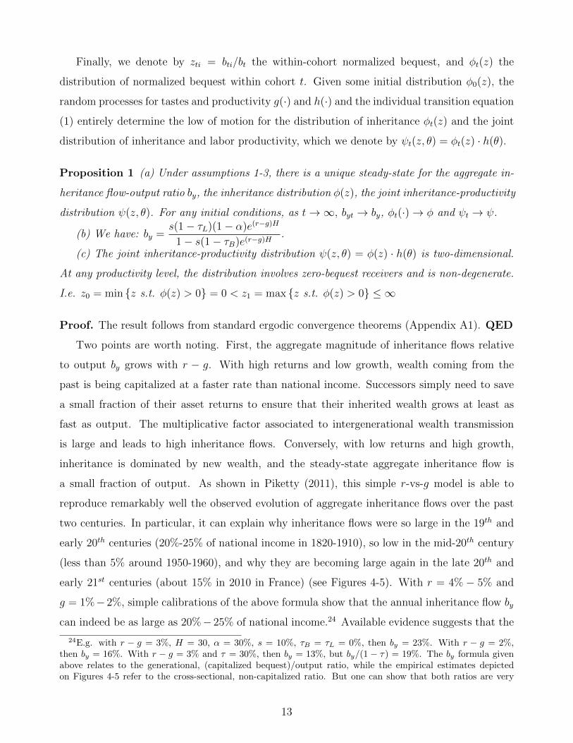


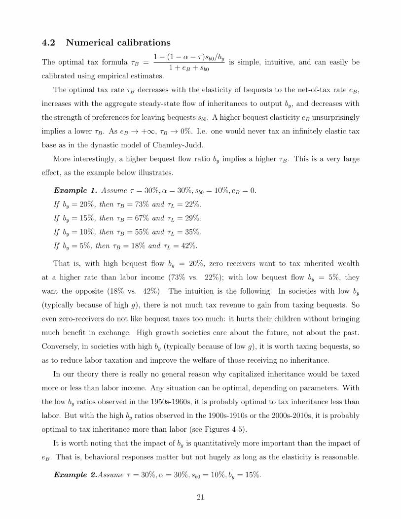
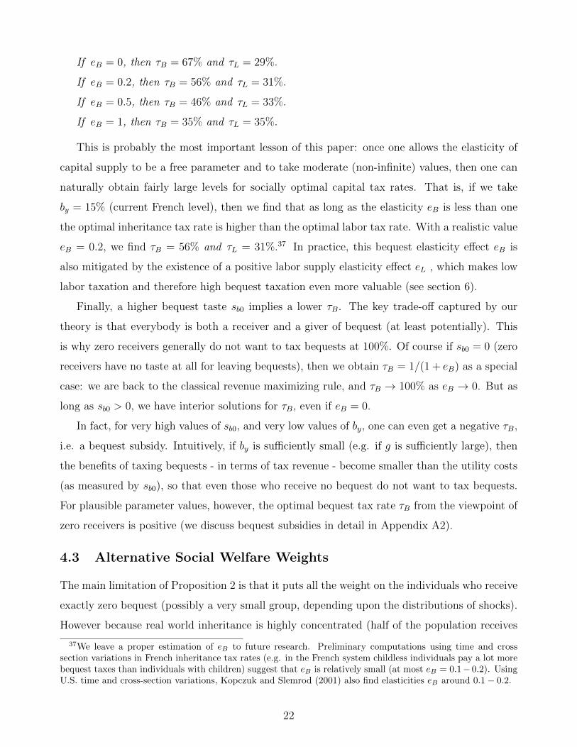


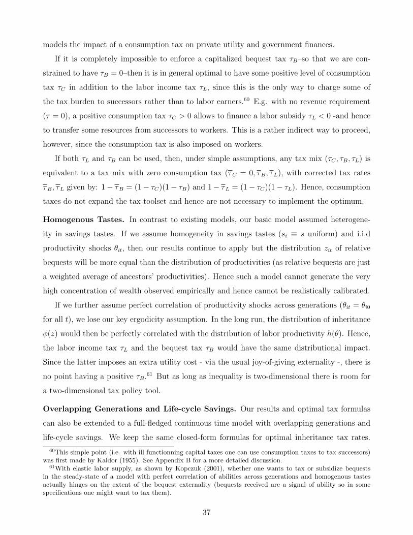


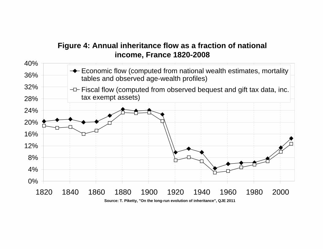
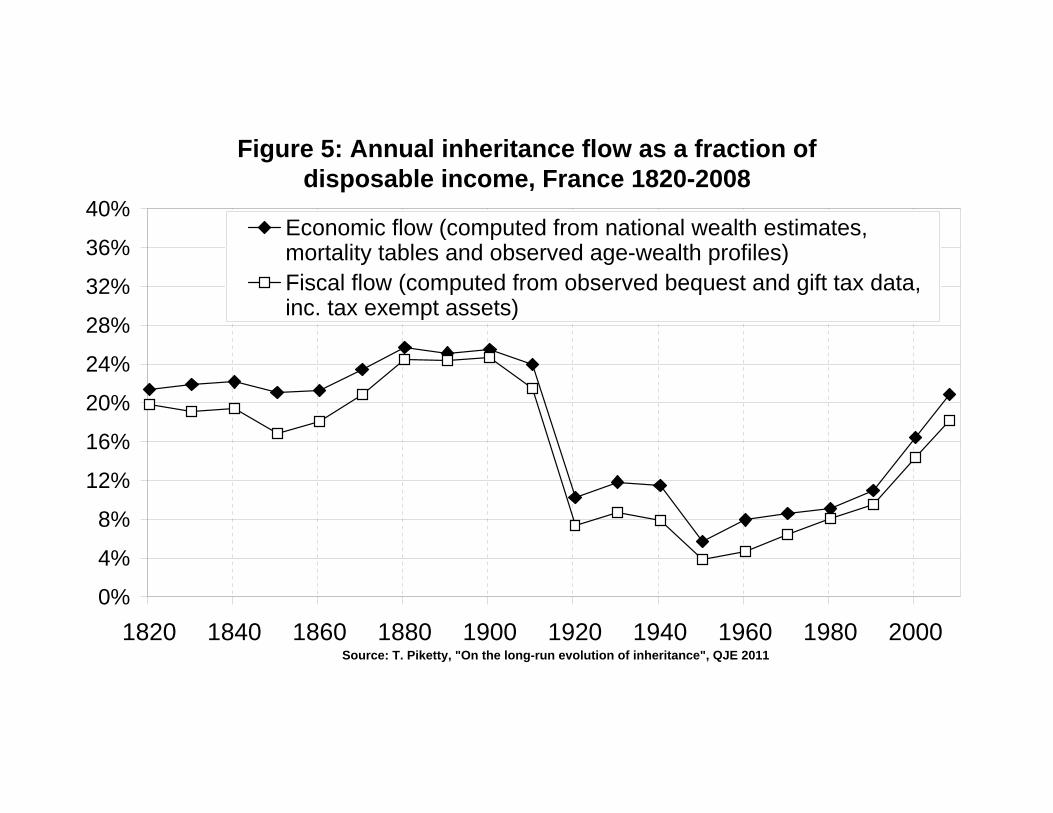


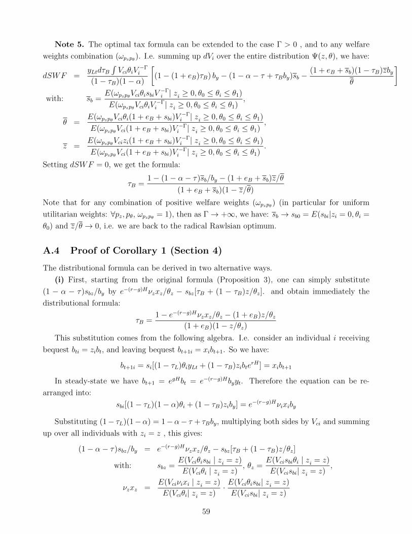
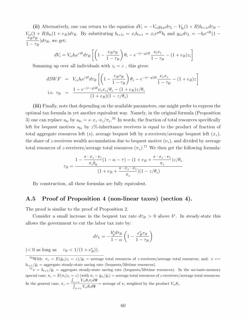


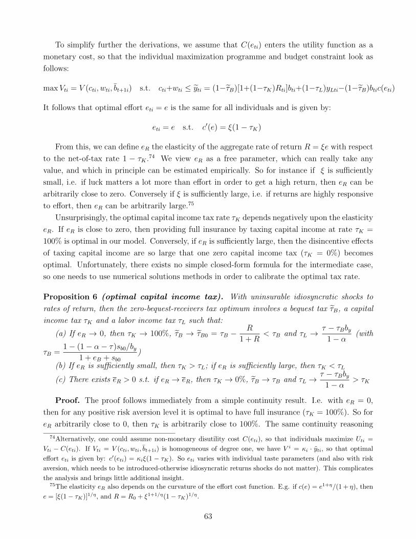


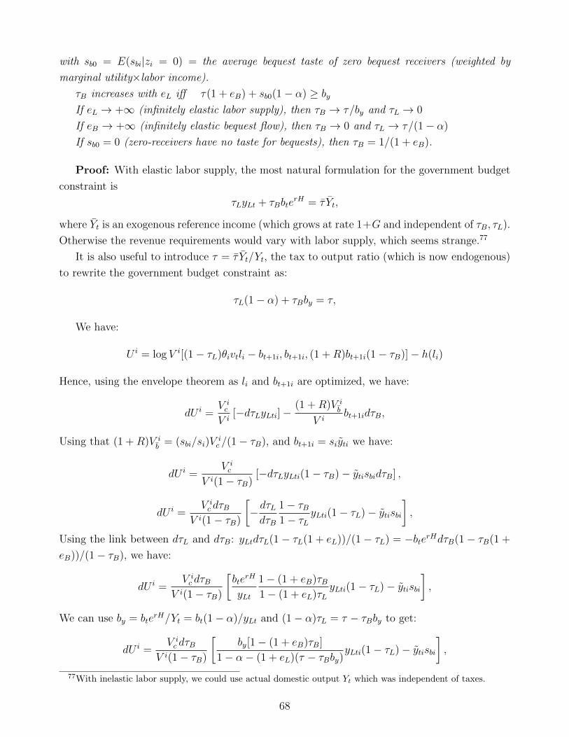


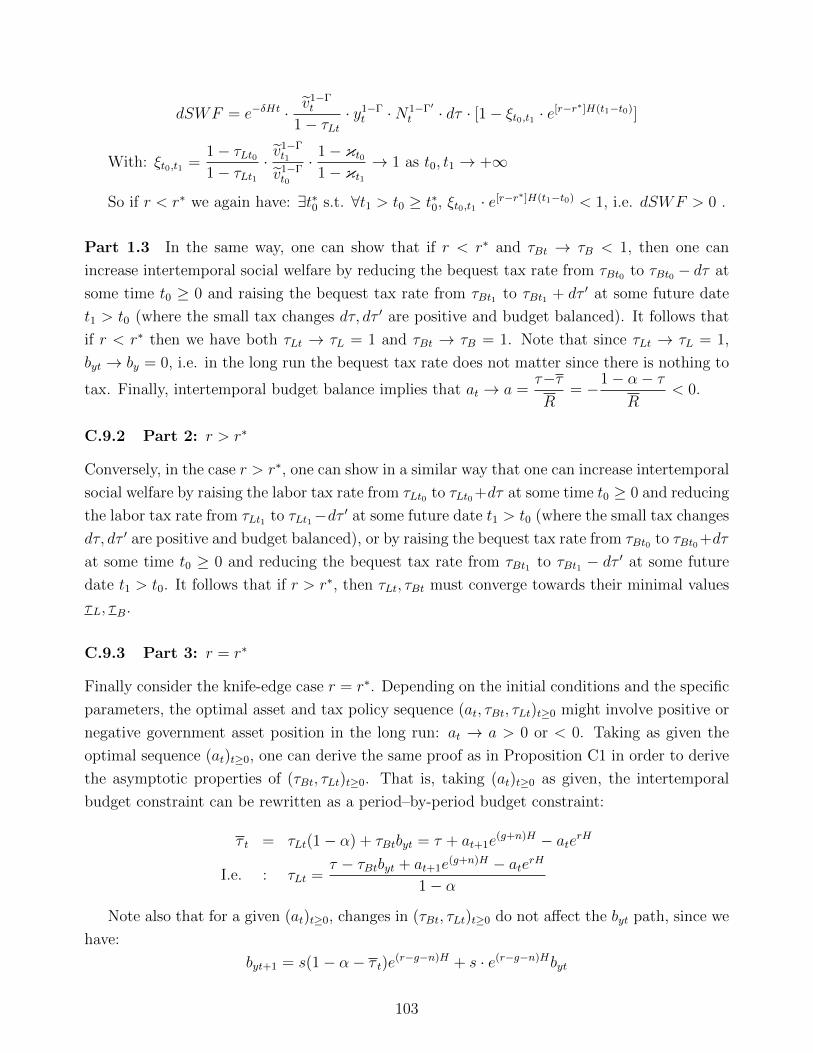


![Income Inequality: Evidence and Policy Implicationselsa.berkeley.edu/~saez/lecture_saez_arrow.pdf · some but not all countries [Atkinson-Piketty-Saez JEL’11] 2) Top tax rates have](https://static.documents.pub/doc/80x56/5e8e0f08107e6a414f603128/income-inequality-evidence-and-policy-saezlecturesaezarrowpdf-some-but-not.jpg)


