A Thermal Profile Method to Identify Potential Ground-Water Discharge Areas and Preferred Salmonid Habitats for Long River Reaches Scientific Investigations Report 2006–5136 Prepared in cooperation with the Bureau of Reclamation, Washington State Department of Ecology, and the Yakama Nation U.S. Department of the Interior U.S. Geological Survey
Transcript
A Thermal Profile Method to Identify Potential Ground-Water Discharge Areas and Preferred Salmonid Habitats for Long River Reaches
Scientific Investigations Report 2006–5136
Prepared in cooperation with the Bureau of Reclamation, Washington State Department of Ecology, and the Yakama Nation
U.S. Department of the InteriorU.S. Geological Survey
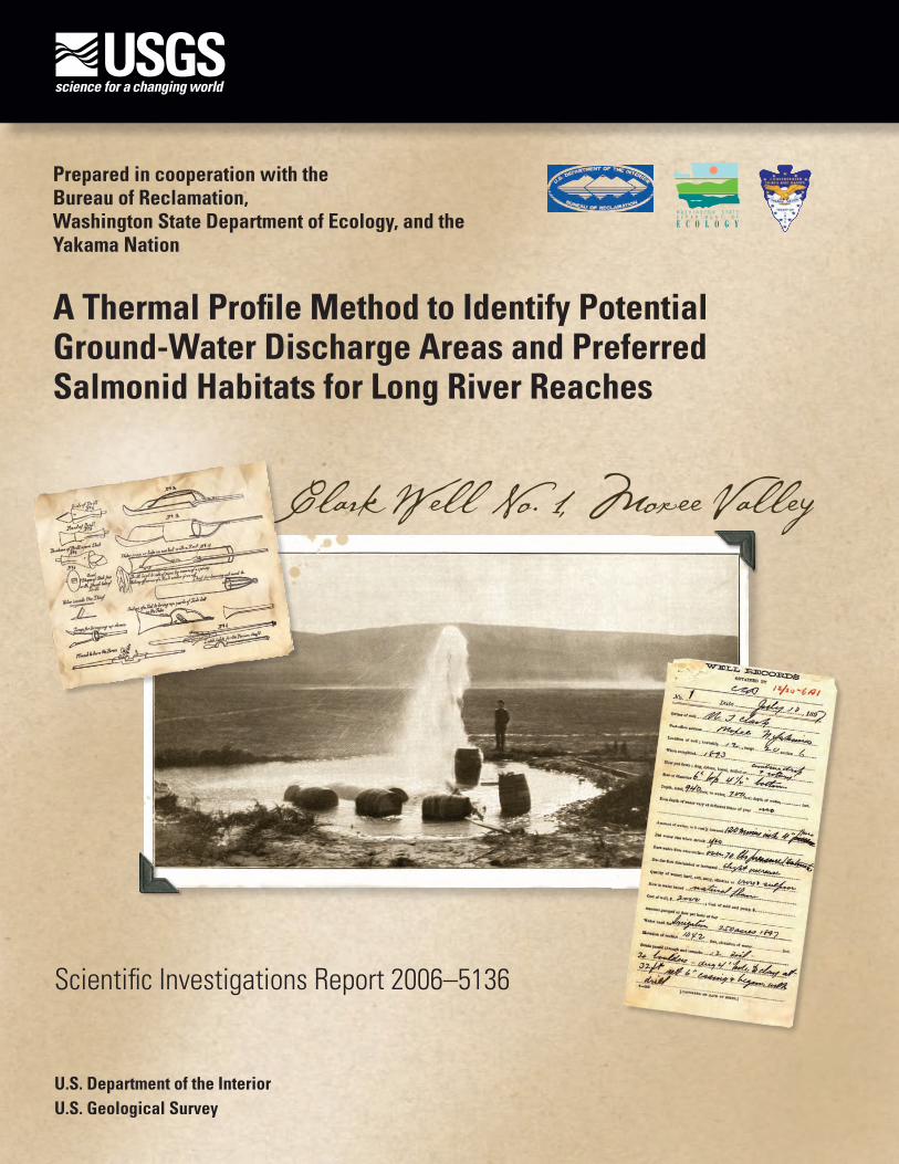
Cover: Photograph of Clark Well No. 1, located on the north side of the Moxee Valley in North Yakima, Washington. The well is located in township 12 north, range 20 east, section 6. The well was drilled to a depth of 940 feet into an artesian zone of the Ellensburg Formation, and completed in 1897 at a cost of $2,000. The original flow from the well was estimated at about 600 gallons per minute, and was used to irrigate 250 acres in 1900 and supplied water to 8 small ranches with an additional 47 acres of irrigation. (Photograph was taken by E.E. James in 1897, and was printed in 1901 in the U.S. Geological Survey Water-Supply and Irrigation Paper 55.)
A Thermal Profile Method to Identify Potential Ground-Water Discharge Areas and Preferred Salmonid Habitats for Long River Reaches
By J.J. Vaccaro, U.S. Geological Survey; and K.J. Maloy, Oregon State University
Prepared in cooperation with the Bureau of Reclamation, Washington State Department of Ecology, and the Yakama Nation
Scientific Investigations Report 2006-5136
U.S. Department of the InteriorU.S. Geological Survey
U.S. Department of the InteriorDirk A. Kempthorne, Secretary
U.S. Geological SurveyP. Patrick Leahy, Acting Director
U.S. Geological Survey, Reston, Virginia: 2006
For sale by U.S. Geological Survey, Information Services Box 25286, Denver Federal Center Denver, CO 80225
For more information about the USGS and its products: Telephone: 1-888-ASK-USGS World Wide Web: http://www.usgs.gov/
Any use of trade, product, or firm names in this publication is for descriptive purposes only and does not imply endorsement by the U.S. Government.
Although this report is in the public domain, permission must be secured from the individual copyright owners to reproduce any copyrighted materials contained within this report.
Suggested citation:Vaccaro, J.J., and Maloy, K.J., 2006, A thermal profile method to identify potential ground-water discharge areas and preferred salmonid habitats for long river reaches: U.S. Geological Survey Scientific Investigations Report 2006-5136, 16 p.
Example of Method Application ……………………………………………………………… 8Background ……………………………………………………………………………… 8Thermal Profile ………………………………………………………………………… 9
Summary and Conclusions …………………………………………………………………… 13References Cited ……………………………………………………………………………… 13
Figures Figure 1. Map showing location of Yakima River Basin, Washington ……………………… 2 Figure 2. Photograph of temperature probe, container, and partially
disassembled container ………………………………………………………… 6 Figure 3. Graph showing example of time-plotted thermal profiles, August 8 and
September 13, 2001, Yakima River Basin, Washington …………………………… 9 Figure 4. Graph showing example of distance-plotted thermal profiles, August 8 and
September 13, 2001, Yakima River Basin, Washington …………………………… 9 Figure 5. Graph showing thermal profile and depth for the cooling part of the example
reach, August 8, 2001, Yakima River Basin, Washington ………………………… 11 Figure 6. Map showing example of thermal profiled reach and salmon redd locations
overlaid on an infrared image, Yakima River Basin, Washington ………………… 12
iv
Conversion Factors, Datums, and Abbreviations and Acronyms
Conversion Factors
Multiply By To obtain
centimeter (cm) 0.3937 inchcubic meter per second (m3/s) 35.31 cubic foot per secondkilometer (km) 0.6214 milekilometer (km) 0.5400 mile, nauticalmeter (m) 3.281 footmeter per second (m/s) 3.281 foot per secondsquare kilometer (km2) 0.3861 square mile
Temperature in degrees Celsius (ºC) may be converted to degrees Fahrenheit (ºF) as follows:
°F=(1.8×°C)+32.
Specific conductance is given in microsiemens per centimeter at 25 degrees Celsius (µS/cm at 25ºC).
Datums
Vertical coordinate information in referenced to the North American Vertical Datum of 1988 (NAVD 88).
Horizontal coordinate information is referenced to the North American Datum of 1983 (NAD 83).
Altitude, as used in this report, refers to distance above the vertical datum.
Abbreviations and Acronyms
Abbreviations and Acronyms Definition
FLIR Forward-looking infrared radiometerGPS Global Positioning SystemLTC Laptop computerWAAS Wide Area Augmentation System
AbstractThe thermal regime of riverine systems is a major
control on aquatic ecosystems. Ground water discharge is an important abiotic driver of the aquatic ecosystem because it provides preferred thermal structure and habitat for different types of fish at different times in their life history. In large diverse river basins with an extensive riverine system, documenting the thermal regime and ground-water discharge is difficult and problematic. A method was developed to thermally profile long (5-25 kilometers) river reaches by towing in a Lagrangian framework one or two probes that measure temperature, depth, and conductivity. One probe is towed near the streambed and, if used, a second probe is towed near the surface. The probes continuously record data at 1-3-second intervals while a Global Positioning System logs spatial coordinates. The thermal profile provides valuable information about spatial and temporal variations in habitat, and, notably, indicates ground-water discharge areas.
This method was developed and tested in the Yakima River Basin, Washington, in summer 2001 during low flows in an extreme drought year. The temperature profile comprehensively documents the longitudinal distribution of a river’s temperature regime that cannot be captured by fixed station data. The example profile presented exhibits intra-reach diversity that reflects the many factors controlling the temperature of a parcel of water as it moves downstream. Thermal profiles provide a new perspective on riverine system temperature regimes that represent part of the aquatic habitat template for lotic community patterns.
1U.S. Geological Survey.
2Oregon State University.
IntroductionIn many basins in the western United States, on-
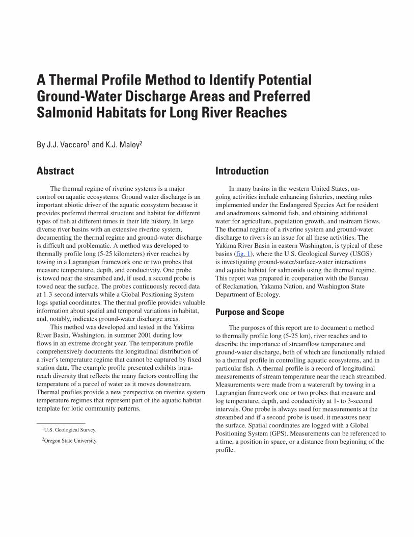
going activities include enhancing fisheries, meeting rules implemented under the Endangered Species Act for resident and anadromous salmonid fish, and obtaining additional water for agriculture, population growth, and instream flows. The thermal regime of a riverine system and ground-water discharge to rivers is an issue for all these activities. The Yakima River Basin in eastern Washington, is typical of these basins (fig. 1), where the U.S. Geological Survey (USGS) is investigating ground-water/surface-water interactions and aquatic habitat for salmonids using the thermal regime. This report was prepared in cooperation with the Bureau of Reclamation, Yakama Nation, and Washington State Department of Ecology.
Purpose and Scope
The purposes of this report are to document a method to thermally profile long (5-25 km), river reaches and to describe the importance of streamflow temperature and ground-water discharge, both of which are functionally related to a thermal profile in controlling aquatic ecosystems, and in particular fish. A thermal profile is a record of longitudinal measurements of stream temperature near the reach streambed. Measurements were made from a watercraft by towing in a Lagrangian framework one or two probes that measure and log temperature, depth, and conductivity at 1- to 3-second intervals. One probe is always used for measurements at the streambed and if a second probe is used, it measures near the surface. Spatial coordinates are logged with a Global Positioning System (GPS). Measurements can be referenced to a time, a position in space, or a distance from beginning of the profile.
A Thermal Profile Method to Identify Potential Ground-Water Discharge Areas and Preferred Salmonid Habitats for Long River Reaches
By J.J. Vaccaro1 and K.J. Maloy2
82 22
22
97
97
97
12
12
82
82
240
24
410
240
90
90
90
24
410
12
97
12
241
82
82 12
KITTITAS COUNTY YAKIMA COUNTY
CO
UN
TYB
ENTO
N
CO
UN
TY
CO
UN
TY
KLICKITATYAKIMA
EXPLANATIONBOUNDARY OF YAKIMA RIVER BASIN
Canal
Roza
Sunnyside
Canal
Main Canal
Extension
KennewickMain Canal
Marion Drain
NorthBranchCanal
Kittitas
Main Canal
BumpingLake N Fk
S Fk
S Fk
N Fk
S Fk N Fk
N Fk
Cle E
lum
Rive
r
Swau
kC
reek
Carib
ouCr
Col
eman
Cr
Nan
eum
Cr
Cook
e Cr
Crow Creek
Bumping Rive
r
American River
Rattlesnake Cr
LittleRattlesnake Cr
Nile Creek
Manastash
BadgerCreek
Lmuma Cr
Ahtanum Creek
Oak Creek
Tieton River
Wide Hollow Cr
Wenas CreekSelah Creek
North Fork
Dry Creek
SimcoeCreek
Agency Creek
Creek
Toppenish
Corral Cr RIVERSpring Cr
Logy
Creek
Satu
s
Creek
MuleDry
Cre
ek
CleElumLake
RimrockLake
KachessLake
KeechelusLake
LakeWallula
PriestRapidsLake
TeanawayRiver
Reecer Cr
Wils
onCr
eek
Park
Cr
Taneum Creek
Umtanum Creek
Little Naches River
Cr
Cowiche Creek
Cowiche Cree
k
River
Naches
Snip
esC
r
Sulp
hu
r Cr Wasteway
CherryCr
S Fk
N
Fk
YAKIMA
YAKIMA
RIVER
Cle Elum
Parker
Wapato
Ellensburg
Umtanum
Kittitas
Thrall
Toppenish
Moxee City Union
Gap
Yakima
Selah
Naches
SunnysideRichland
Kiona
KennewickProsser
Grandview
Mabton
Satus
Zillah
Granger
Roza
Easton
Teanaway
TietonRimrock COLUMBIA
RIVER
SnoqualmiePass
Van Epps Pass
EsmeraldaPeaks
K I T T I T A S
V A L L E YM A N A S T A S H
KACHESSRIDGE
R I D G E
UNION GAP
CLEMAN MOUNTAIN
TEANAW
AY
NORTH RIDGE
U M T A N U M
R I D G E
DeceptionPass
Y A K I M A
V A L L E Y
AHTANUM RIDGE
COWICHE MTN
AMERICAN RIDGE
CLEELUM
RIDGE
RIDGE
TOPPENISH RIDGE
R A T T L E S N A K EH I L L S
Y A K I M A
R I D G E
H O R S EH E A V E N
H I L L S
CA
SC
AD
ER
AN
GE
WE N AT C H E E
M O U N TA I N S
GilbertPeak
121°
47°
47°30'
46°
120°121°30' 120°30' 119°30'
46°30'
0 5 10 20 30 40 MILES
0 5 10 20 30 40 50 60 KILOMETERS
YakimaRiverBasin
WASHINGTON
waA4WT1_03_fig01
Figure 1. Location of Yakima River Basin, Washington.
� Thermal Profile Method to Identify Potential Ground-Water Discharge Areas
The report first presents a background on the ecological importance of temperature and ground-water discharge in riverine systems and the methods typically used to measure these two environmental variables. The newly developed method to thermally profile reaches is then described. Last, an example of a thermal profile is presented and discussed to provide readers with an overview of a profile, including its information content, how a profile may be interpreted, and the reproducibility of the results using this method. To the extent possible, references and discussions are related back to the importance of temperature as a resource for fish, and in particular salmonids.
Background
Processes that control the heat content of a parcel of surface water as it travels from headwaters to a river mouth are well documented. The processes include radiation, advection, conduction, evaporation, and convection (Anderson, 1954; Harbeck and others, 1959; Raphael, 1962; Messinger, 1963; Koberg, 1964; Edinger and Geyer, 1968; Edinger and others, 1968; Stevens and others, 1975; Jobson, 1977; Sinokrot and Stefan, 1993). Ground-water discharge represents a significant form of thermal advection in many river systems. Ground-water discharge (including water discharged from the hyporheic zone) (1) provides preferred thermal structure and habitat for different types of fishes at different life-history stages (Power and others, 1999), and (2) is an important abiotic variable of the aquatic ecosystem basic to the ecological function of riverine systems (Hynes, 1983; Stanford and Ward, 1993; Stanford and Simons, 1992; Brunke and Gonser, 1997). The ground- and surface-water interface is a unique ecotone and is similar to other ecotones known as some of the most productive habitats (Wetzel, 1990). Much of the year, streamflow is mostly baseflow—a product of ground-water discharge; therefore, water quality also is largely influenced by ground water. An overview of the current understanding of the interaction between ground water and surface water is presented in Winter and others (1998).
Temperature
Role in River EcologyTemperature is one of the most important abiotic
variables of the riverine system because it influences dissolved oxygen concentrations, photosynthesis, the metabolic rates of aquatic organisms, timing of life-history stages of many species, and the decomposition rates of organic material, which in turn, affect the spatial arrangement in the riverine system of many ecosystem components such as algal, invertebrate, and fish communities. Therefore, the bioenergetics of riverine ecosystems ultimately is determined
by the thermal regime. The presence of diversity and structure in the temperature regime leads to increased biodiversity (Magnuson and others, 1979), including biodiversity of fish (Brett, 1956; Beschta and others, 1987), insects (Vannote and Sweeney, 1980), and macrophytes (Haslam, 1978; White and others, 1987). Diversity represents long temporal variations from expected heating trends (overall thermal profile shape—longitudinal gradient) and structure represents the short spatial-temporal variations (the spikes in the thermal profile). Diversity and structure display unique spatial patterns that are functionally related to ground-water discharge. In turn, the variations in the thermal diversity and structure increase with basin size and attendant variations in climatic regimes and landscape characteristics—an upland 5 km2 headwater basin has much less variation than a large 12,000 km2 basin.
Diversity in a basin’s thermal regime represents the riverine system’s temperature template or longitudinal gradient, which is consistent with an environmental gradient. Temperature essentially defines a physical habitat template (Southwood, 1977; Poff and Ward, 1990) that explicitly includes temporal variability and provides for the overall biological community template—including the different life stages and life history patterns of salmonids. The template leads to a logical progression of the longitudinal gradient of fish assemblages. Small scale temperature variations (structure) represent cooling patches (possible refugia) or heating (avoidance areas) overlaid on the basin-wide template, and reflect the localized lateral and vertical connections measured in both natural and modified river systems (Hynes, 1983; Stanford and Ward, 1993) that salmonids use or avoid (Power and others, 1999; Rieman and Dunham, 2000). These ground-water discharge zones provide refugia, the preferred salmonid habitat during summer when river temperatures are warm and during winter in colder regions when rivers may freeze. Salmonids seek out and take advantage of this habitat. The longitudinal gradient, overlaid with the distribution of patches, composes a continuum from the headwaters to the mouth, along which habitat and species are arranged (Vannote and others, 1980).
The thermal regime at salmon redds (gravel spawning nests) also is important for incubation (Combs and Burrows, 1957; Combs, 1965; Alderdice and Velsen, 1978). The thermal regime and ground-water discharge effects egg survival for salmonid species (Sowden and Power, 1985; Woessner and Brick, 1992: Curry and others, 1995) including wild bull, rainbow, steelhead, and kokanne trout in the Yakima River Basin. Ground-water discharge areas also appear to be the preferred winter habitat for trout (Brown and Mackay, 1995), and temperature habitat limitations may affect behavior (Gregory and Griffith, 1996). Power and others (1999) identified winter as critical time (1) when overwintering fish mortalities may be high and (2) in the establishment of basic stock densities based on temperature habitat availability.
Introduction �
MeasuringIn large diverse basins with an extensive riverine system,
documenting the thermal regime is difficult. Methods typically used to document the regime are continuous measurements at fixed stations, synoptic manual measurements, and multi-spectral imaging. Fixed station and synoptic data measure only heat content of a particular water parcel, so information on the spatial structure of the thermal regime, which describes a habitat template, must be interpolated. However, accurate interpolation requires additional measurements (longitudinal, transverse, and advectional) to quantify thermal variation in a stream. Using multi-spectral techniques such as forward-looking infrared radiometer (FLIR) can yield the thermal regime of a riverine system, but only for one period, and these methods are costly and synoptic. How the regime varies temporally is unknown. Moreover, FLIR measures surface radiance and does not document vertical structure. As a result, excluding features such as springbrooks, ground-water discharge cannot be precisely located with FLIR until manifested at the water surface.
Measuring Ground-Water DischargeSeveral methods are used for quantifying ground-
water discharge in riverine systems. The most common method is to make a series of discharge measurements. Such measurements provide useful information on net gain or loss in a reach defined by the bounding measuring sites for some particular time. When used in conjunction with dye-dilution gaging measurements (Kilpatrick and Cobb, 1985), discharge measurements also can provide information on ground-water discharge and recharge (sum equals net gain or loss) over a reach (Harvey and Wagner, 2000). In large systems, many discharge measurements, which can be costly, are needed to identify ground-water discharge locations, especially in extensively modified systems or when investigating the temporal variability in the discharge.
Seepage meters were used in lake studies to measure ground-water discharge (Lee, 1977; Lee and Cherry, 1978). Seepage meters are best suited for sandy lakeshores, and installation in rivers is problematic (Lee and Hynes, 1978; Harvey and Wagner, 2000). Using mini-piezometers was described early in the literature and has been oriented to studies of salmonid habitat (Terhune, 1958; Gangmark and Bakkala, 1958; Coble, 1961; Vaux, 1962). This method was modified for the reach survey using manometer-style measurements (Fokkens and Weijenberg, 1968; Lee and Cherry, 1978; Winters and others, 1988), which use mini-piezometers to measure the pressure head in shallow ground water with a concurrent measurement of the river head; these
are done conjunctively using a portable manometer. Detailed information is provided by such surveys. For example, Simonds and others (2004) determined that, for some gaining reaches in the Dungeness River, Washington, identified from discharge measurements at bounding sites, the river was losing water over most of the reach and the ground-water discharge was local. Jackman and others (1997) measured large variations in discharge across the width of a small stream. Data presented in White and others (1987) also suggested variations in discharge across a 7-m wide river.
Monitoring of streamflow and vertical distribution of temperature below the streambed (Lapham, 1989; Silliman and Booth, 1993; Constanz, 1998; Constanz and others, 2001) yielded data for estimating ground-water discharge. Such monitoring with concurrent modeling provided detailed ground- and surface-water interactions at the diurnal to seasonal scale. The method is most easily applied to the ephemeral and lower order parts of the stream network and is difficult to use in larger stream reaches with high streamflow, especially with limited boat access. As with fixed station data, the usefulness of results are highly dependent on locations selected for monitoring.
Introduced stream tracers can be used to estimate discharge areas (Bencala and Walters, 1983; Jackman and others, 1984; Kilpatrick and Cobb, 1985; Triska and others, 1989). Tracers can include environmental tracers such as temperature (White and others, 1987), and tracer studies may or may not include modeling. Tracers are best applied to short reaches (less than the length scale of the longitudinal dispersion coefficient) and mainly for hyporheic flow analysis (Harvey and Wagner, 2000).
Continuous measurements of water levels and temperature in ground water in shallow piezometers near and in the river also are used to estimate ground-water discharge (or river losses) (Harvey and Wagner, 2000). The latter two methods become intractable over long reaches or for an entire riverine system.
Electrical conductivity profiling also can be used to locate ground-water discharge areas. Lee and others (1997) used two electrodes encased in a tubular shell with a brass nose cone towed from the back of a motorized watercraft. Electrodes were connected to a laptop computer (LTC) by a cable. The electrodes’ output, which was converted to a value of electrical conductivity, was used as a measure of the difference between river water and ground water. Location of the shell was determined by a continously logging GPS. For many riverine systems, using a towed measurement device connected to an LTC would not be applicable due to channel configuration, water depths, rapids, various bottom materials, log-jams, diversion dams, riprap, and partially submerged or buried tree limbs. However, the basic concept of profiling provides a technique that can be modified for most riverine systems.
� Thermal Profile Method to Identify Potential Ground-Water Discharge Areas
Basis for Thermal ProfilingApplying these measuring methods to most large riverine
systems, such as the Yakima River Basin, is challenging because many systems were extensively modified with diversions and return canals, and there are usually thousands of kilometers of stream network. In turn, many parts of such a network may provide habitat for several life-history stages of anadromous and resident salmonids and other fish. To partially address this issue, a method was developed to thermally profile long (about 5-25 km) river reaches. The profile is based on measuring water temperature at 1- to 3-second intervals at or near the streambed, and in some cases, concurrently measuring (profiling) the water temperature near the surface. Measurements are taken in a Lagrangian framework, which entails drifting at the ambient streamflow velocity. This method produces a longitudinal, Lagrangian profile of stream temperature near the streambed.
Electrical conductivity profiling of the cobble-bottom streambed of the Hanford Reach on the Columbia River, Washington, by Lee and others (1997) identified ground-water discharge areas. This method was similar to that of Lee and Dal Bianco (1994), who applied it to a small, gravelly bottom river. The profiling method was based on techniques to locate ground-water discharge areas in lakes (Lee, 1985; improved on by Harvey and others, 1997). Together, these studies demonstrated that profiling is an effective method for locating ground-water discharge areas, especially when combined with piezometer measurements.
The conceptual basis for development of the method was to determine if a robust, thermal-profiling method could be developed, and if so, to document the thermal profile, with its attendant diversity and structure, of selected reaches. Profiles should yield information related to salmonid habitat because the complexity in salmonid life histories is functionally related to diversity in thermal habitat (Rieman and Dunham, 2000). If a thermal profile could be documented, it then needed to be determined if areas of ground-water discharge could be identified from the thermal profile.
Profiling in a Lagrangian framework (moving downstream at the same velocity as the river) allows for tracking temperature of a parcel of water as it moves downstream in a reach. Deviations from the diurnal heating of a parcel should principally be due to ground-water discharge, surface-water inflows, and depending on setting, streamflow losses or riparian-vegetation shading. In particular, deviations (anomalies) from an overall heating response may represent ground-water discharge areas. Using temperature anomalies to identify ground-water discharge areas is not a new concept (e.g., Cartwright, 1970); discharge areas will have a larger vertical thermal gradient than recharge areas. Areas with sharp thermal gradients are candidates for more intensive studies.
Thermal Profile Method
Equipment
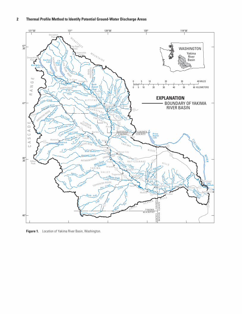
A self-contained temperature measuring and recording probe, encased in stainless steel and designed for ground-water monitoring, was selected as the best option for thermal profiling because no cables are needed to be towed, therefore, preventing damage to or loss of sensor/cable. The probe (CTD-Diver™, Van Essen Instruments; now manufactured by Solinst® and called a Levelogger®) has the added benefits of also measuring conductivity and depth with a variable sample rate. The probe (fig. 2) is 2.2-cm diameter, 26.0-cm long, and weighs 160 grams; an optical read-out unit connected to an LTC is used to program and read out the datalogger.
Probe accuracy was rated as 0.1°C for temperature, 0.1 percent of the full range of depth (in cm), and 0.05 µS/cm for conductivity. The reported accuracy of the probe’s internal clock is better than 1 second per day at 20°C. Temperature measurement reliability was checked using a controlled temperature bath (accuracy of 0.05°C) over a range 6 to 30°C. Results confirmed an accuracy of 0.1°C over the full range and temperature change over 1-second intervals was captured by the probe. A probe that only measures temperature or temperature and depth also can be used in this method.
A light, rugged container consisting of white 5.1 cm plastic pipe with a rounded cap on one end, and a total length of about 38 cm was designed for the probe (fig. 2). Water flowed through 1.5-cm holes drilled throughout the container body. A stainless steel eye bolt on the end of the cap with two bolts provides a connection for a 15-m tow rope. A 15.25-cm piece of 2.5-cm diameter flexible wire conduit is centered in the cap, and a bolt hole is drilled through (perpendicular to) the cap and conduit; a bolt allows for probe attachment. A greased bolt is then inserted and the surrounding area is filled with silicon caulk; greasing the bolt allows for easy bolt removal after the caulk hardens. Caulk helps prevent the bolts on the eyebolt from loosening, holds the conduit in place, and adds weight to the front of the container for towing. About 9 cm of the probe extends into the conduit and the probe extends about 2 cm inside the container end. A neoprene bicycle handle is inserted over the probe extending beyond the conduit (but not covering the sensor) and is held in place with 2.5-cm wide, 10-mil, all weather pipe-wrap tape. The conduit and neoprene prevent the probe from contacting the sides of the container, but allow some movement to absorb shocks when contacting various bottom structures such as boulders. Neoprene also provides some buoyancy needed to allow the container to move around or over a stream’s bottom structure such as large boulders. After many profiles, the container withstood constant contact with the streambed, boulders, woody debris, and other objects.
Thermal Profile Method �
Protocol
One or two probes can be used in this method. Two probes initially were used during method development; currently (2006) one probe is deployed for a profile. If using two probes, one is for streambed measurements and the other is for shallow measurements. If more than one reach is profiled using two probes, for consistency in inter-reach comparison, identify one probe for shallow measurements and the other probe for streambed measurements.
While developing and testing this method, the probe’s sample rate was set at 3 seconds. For conductivity measurements, Harvey and others (1997) used a sample rate of 0.1 sec and Lee and others (1997) used a sample rate of 0.05 sec. The 3-second rate was used based on expected streamflow velocity and initial reach length because measuring temperature every 0.2-6 m would capture
differences representative of large discharge quantities without compromising probe storage capacity and allow for sensor equilibration. However, based on datalogger capacity and profiled reach length with its attendant average velocity, the sample rate (ranging from 1 to 3 seconds) was adjusted for each reach. Expected average velocity for a reach should be analyzed in conjunction with the reach length to estimate a sample rate based on storage capacity of the particular probe and the GPS used. Additionally, if possible, the probe and GPS should use the same sample rate to simplify merging the resulting two data series. A slower sampling rate can be used depending on the specific purpose for measuring a profile. For example, other investigators used this method along a reach with measured large quantities of ground-water discharge and set the sample rate at 6 seconds to identify the area where ground-water discharge begins (G. Gregory, written. commun., Washington State Department of Ecology, 2006).
ProbeProbe
TopTop
BoltBolt
ContainerbottomContainerbottom
AssembledcontainerAssembledcontainer
Attached tow lineAttached tow line
Wrappedneoprenehandle
Wrappedneoprenehandle
FlexableconduitFlexableconduit
Probe top toshow holefor bolt
Probe top toshow holefor boltAttached
boltAttached
bolt
waA4WT1_03_fig02
Figure �. Temperature probe, container, and partially disassembled container.
� Thermal Profile Method to Identify Potential Ground-Water Discharge Areas
Two methods were used to determine the location of the watercraft towing the CTD-Diver™. First, a Garmin 76 GPS was connected to a LTC using Garmin’s MapSource™ software. MapSource™ enables streaming of GPS data to a stored route at a 1-second sample rate. Each GPS data point on the route is time stamped, and latitude, longitude, altitude, and for each leg between readings, the length, speed, and course are recorded. For this method, the LTC was placed in a waterproof container and the GPS was placed in a smaller container bolted to the top of the LTC container and sealed with caulk. An opening between the two containers allowed for cable connection between the GPS and LTC. The LTC operated from a small gel-cell battery through an inverter that makes a warning sound when the battery is low. Two back-up batteries should be carried in waterproof bags.
Second, a Trimble® GeoXM™, operating with TerraSync™ and Geoexplorer CE™ software, was used. This method does not require an LTC in the watercraft, and the GeoXM™ collects GPS coordinates at a user-defined time interval and accuracy. Both GPS units are WAAS (Wide Area Augmentation System) enabled and when receiving the WAAS signal, the horizontal accuracy generally is less than 3 m (15 m without WAAS). The Garmin® set-up from the first method also was used to synchronize the clock in the probe to GPS time.
To start a profile, the LTC’s time is set to GPS time using the Garmin® and its software. The probe’s internal clock is then set to the LTC’s time, closely synchronizing it to GPS time. Start times and sample rate of the probe or probes are then set.
The probe or probes are then placed in the water for at least 5 minutes to equilibrate to the ambient water temperature. Equilibration is needed because the combined mass of the probe and container affects the measured temperature when a large temperature differential exists between the probe/container and streamflow. For example, on a warm day, the probe and the container may obtain an ambient temperature of 35°C during transport to a site and streamflow temperature may be 15°C. Starting a profile with such a differential would result in a sensor slowly equilibrating to streamflow temperature. After equilibrating to near ambient streamflow temperature, the semiconductor sensor is unaffected by the probe and container temperature.
Next, either the Garmin® GPS was connected to the LTC and a route was started with data logging or the GeoXM™ was started for data logging a line feature. A profile was then started with the shallow probe (if one is used) just under the water surface and the deep probe hand held with a towline. The deep probe is hand held for safety reasons. For example, if an attached tow line was snagged in fast current, the watercraft could become submerged or capsize. Although not done for this study, a small buoy can be attached to the towline. The buoy would allow towline recovery if it is lost. Profiling is as continuous as possible to avoid temporal discontinuities due to
the water-temperature increases during the time the profiling is suspended. Profiles are best completed at lower flows, staying near the thalweg.
Last, temperature dataloggers were deployed at the head and tail of the profiled reach. Temperature data from these loggers provided additional information on the diurnal temperature change in water entering and leaving the reach. The difference between upstream temperature and thermal profile also provided information on variations from the expected warming of a water parcel. These differences relate to the change in the heating rate.
The type of watercraft used usually depends on physical characteristics of a particular reach and streamflow volume. Profiling was completed over a wide range of flows, about 1 to 110 m3/s. During the method’s initial development, a two-man inflatable raft with a rowing platform was used. To obtain greater mobility and control, a two-person, self-bailing inflatable kayak was used instead of the raft and was a good work platform. A motorized watercraft was used for one reach, but because it did not provide as much control as a kayak for measuring in a Lagrangian framework, it was determined that motorized watercraft is best suited for non-braided reaches with streamflow velocities less than about 0.2 m/s. Other investigators using this method have used a single-seat, inflatable pontoon watercraft (G. Gregory, Washington State Department of Ecology, written. commun., 2006), which also should be a good working platform.
Time required to profile a reach depends on reach length, average velocity, and potential impediments such as diversion dams or log jams. Profiling a reach of about a 5 km starts at about 10:00-11:00 a.m., and for longer reaches profiling generally starts as early as 8:30 a.m. to ensure that diurnal heating is strongly initiated. Ideally, reaches are profiled on cloudless days. Shorter reaches with lower streamflow volumes can be profiled by wading. A handheld GPS with data logging capabilities is the best instrument to use for waded reaches.
Limiting Factors
Profiling in a Lagrangian framework at velocities as much as 2.0 m/s results in the sensor moving rapidly over the streambed. In turn, low volumes of ground-water discharge results in a high volume of stream water contacting the sensor compared to ground water. Therefore, a high-resolution survey of temperature variations due to ground-water discharge at the streambed is not documented using this method. Testing the potential to conduct high-resolution surveys indicated the method would work, but the maximum drift velocity should be less than about 0.20-0.25 m/s. This conclusion however, is based on conditions during the profiling while developing and testing the thermal-profiling method. For neutral or losing parts of reaches, the thermal profile resolution generally is good and is a function of combined effects of the sampling interval and streamflow velocity.
Thermal Profile Method �
Another limiting factor is that a particular volume of water measured may not be representative of streambed water in ground-water discharge areas due to mixing. Mixing can mask the ground-water signature and is affected by channel morphology and streamflow volume and velocity. Probe location relative to the streambed also varies. Problems with the actual location of measurements arise because the tow-line length can change (0.5-3 m) to keep the probe as close to the raft as possible for accurate GPS locations while attempting to stay at the streambed. Length also is changed when moving through rapids, areas of woody debris, and riprap or to avoid submerged objects that can snag the streambed probe. These tasks are difficult in fast-moving current and rapidly changing bottom conditions. Therefore, the accuracy of the measurement location is reduced, but the position is accurate when referenced to the nearby logged positions. Of the tens of thousands of measurements made during the method testing and use, relatively few were upstream of the previous recorded position and few were on the stream bank. More challenging is the loss of GPS reception, in which case, the latitude and longitude are linearly interpolated between GPS values that bracket that period and are then assigned to the CTD data. This method produces a straight line track, which may not represent that part of a reach. However, Geographic Information System (GIS) can be used to fit the track to the channel center to improve accuracy of the profile location.
The nature of ground-water discharge also can confound profiling results because discharge can occur as low-volume diffuse to high-volume spring, and older, and perhaps colder ground water near the thalweg compared to younger, perhaps warmer, ground water near channel edges (Modica and others, 1997).
A thermal profile documents a linear track of temperature and does not capture any three-dimensional aspects of the thermal regime in a reach. However, areas of interest are readily identified. These areas can be investigated in more detail using discharge measurements in conjunction with mini-piezometer measurements.
Example of Method Application
Background
Initial profiling in the Yakima River Basin was done July through September 2001, an extreme drought year, when heat flux was large and the difference between temperature of ground water and stream water should be greatest, especially for downstream, low-gradient reaches of this large riverine system. Drought led to lower than average streamflows and greatly decreased (in some cases eliminated due to demand) surface-water agricultural return flows; nonetheless,
measured low flows were relatively large (between about 8.6 to 9.2 m3/s in the example reach) compared to low flows in many river systems. Methods were checked and a protocol, described above, was developed during the initial profiling. Other profiles have been completed for reaches based on the methods and protocols described in this report. For the other profiles, streamflow temperatures ranged from 2 to 24°C and velocities ranged from nearly 0 to as much as 1.8 m/s.
Profiling a reach was timed to coincide with the lowest summer flows for a reach based on operation of reservoirs in the basin, and, when possible to coincide with the building of redds by anadromous spring Chinook salmon. Summer also is important for other life-history stages of salmonids, and temperature is identified as a limiting factor in some reaches (Systems Operations Advisory Committee, 1999). Physiological functions of salmonids are impaired when temperatures are greater than their preferred range (Beschta and others, 1987).
Two contiguous reaches profiled in August were re-profiled in September to (1) verify that results from the method are reproducible; (2) determine the types of differences that may occur under two different heat fluxes; and (3) re-examine a long stretch of the reach with potential ground-water discharge noted during the August profiling. Results for one reach profiled on August 8 and September 13, 2001, are presented as an example of the profiling method to highlight information contained in the profile data related to diversity, structure, and reproducibility of measurements, and to show how profiles may be analyzed, interpreted, and presented.
For August and September, maximum and minimum air temperatures were similar near the upstream part of the reach and maximum and minimum air temperatures were lower during September at the downstream part of the reach. Maximum air temperatures were about 34°C at 16:45 in August and 14:15 in September. Cooler reservoir water released in September, combined with cooler nighttime temperatures, resulted in slightly cooler water entering the reach compared to August. In August and September, the streamflow temperatures entering the reach varied by only 0.36 and 0.32°C, respectively, during profiling; these small variations are due to the large volume of reservoir releases to meet diversions just upstream of the example reach. The profiled reach is just below two large diversions, with streamflows about 66 m3/s for August and 51 m3/s for September.
The example reach was nearly 23 km with an average depth of about 90 cm; the reach has a gradient lower than headwater reaches, a highly braided channel, and a reasonably intact floodplain. Bed sediment in this reach is used by or otherwise suitable for anadromous salmonid (autumn chinook stock and coho) spawning and by several salmonid for pre-spawning holding, rearing, and emigration.
� Thermal Profile Method to Identify Potential Ground-Water Discharge Areas
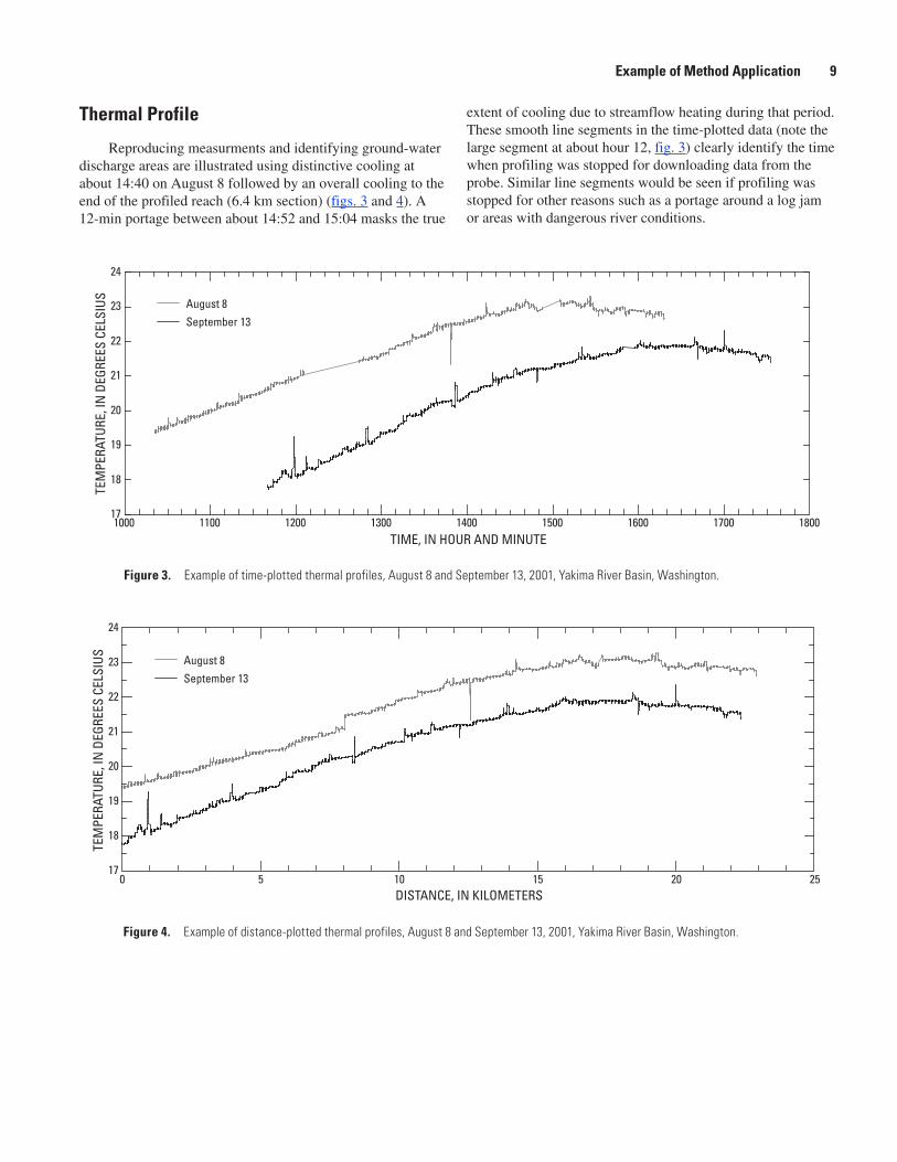
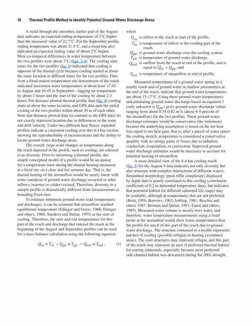
Thermal Profile
Reproducing measurments and identifying ground-water discharge areas are illustrated using distinctive cooling at about 14:40 on August 8 followed by an overall cooling to the end of the profiled reach (6.4 km section) (figs. 3 and 4). A 12-min portage between about 14:52 and 15:04 masks the true
extent of cooling due to streamflow heating during that period. These smooth line segments in the time-plotted data (note the large segment at about hour 12, fig. 3) clearly identify the time when profiling was stopped for downloading data from the probe. Similar line segments would be seen if profiling was stopped for other reasons such as a portage around a log jam or areas with dangerous river conditions.
Figure �. Example of time-plotted thermal profiles, August 8 and September 13, 2001, Yakima River Basin, Washington.
Figure �. Example of distance-plotted thermal profiles, August 8 and September 13, 2001, Yakima River Basin, Washington.
waA4WT1_03_fig03
17
18
19
20
21
22
23
24
1000 1100 1200 1300 1400 1500 1600 1700 1800TIME, IN HOUR AND MINUTE
TEM
PERA
TURE
, IN
DEG
REES
CEL
SIUS August 8
September 13
waA4WT1_03_fig04
17
18
19
20
21
22
23
24
0 5 10 15 20 25DISTANCE, IN KILOMETERS
TEM
PERA
TURE
, IN
DEG
REES
CEL
SIUS August 8
September 13
Example of Method Application �
A trend through the smoother, earlier part of the August data indicates an expected ending temperature of 2°C higher than the measured value of 22.7°C. For the September profile, ending temperature was about 21.4°C, and a trend line also indicated an expected ending value of about 2°C higher. Most co-temporal differences in water temperature between the two profiles were about 2°C (figs. 3-4). The cooling start times for the two profiles (fig. 3) indicated that cooling is opposite of the diurnal cycle because cooling started at about the same location at different times for the two profiles. Data from a fixed-station temperature site downstream of the reach indicated maximum water temperatures at about hour 17:45 in August and 16:45 in September—lagging air temperature by about 2 hours and the start of the cooling by about 2-3 hours. For distance-plotted thermal profile data (fig. 4) cooling starts at about the same location, and GPS data puts the initial cooling of the two profiles within about 30 m of each other. Note that distance-plotted data (in contrast to the GPS data) do not exactly represent location due to differences in the route and drift velocity. Under two different heat fluxes, repeated profiles indicate a consistent cooling over this 6.4 km section, showing the reproducibility of measurements and the ability to locate ground-water discharge areas.
The overall, large-scale changes in temperature along the reach depicted in the profile, such as cooling, are referred to as diversity. Prior to measuring a thermal profile, the simple conceptual model of a profile would be an analog for a temperature trace during the diurnal heating measured at a fixed site on a clear and hot summer day. That is, the diurnal heating of the streamflow would be nearly linear with some variations if ground-water discharge occurred or other inflows (warmer or colder) existed. Therefore, diversity in a sample profile is dramatically different from measurements at bounding fixed sites.
To estimate minimum ground-water load (temperature and discharge), it can be assumed that streamflow reached equilibrium temperature (Edinger and Geyer, 1968; Edinger and others, 1968; Sinokrot and Stefan, 1993) at the start of cooling. Therefore, the start and end temperatures for this part of the reach and discharge that entered the reach at the beginning of the August and September profiles can be used for a mass-balance calculation using the following equation
Q T Q T Q Tin in gw gw out out× × ×+ = , (1)
where Qin is inflow to the reach at start of the profile, Tin is temperature of inflow to the cooling part of the
reach, Qgw is ground-water discharge over the cooling system, Tgw is temperature of ground-water discharge,
Qout is outflow from the reach at end of the profile, and is equal to Q Qin gw+ , and
Tout is temperature of streamflow at end of profile.
Measured temperatures of a ground-water spring in a nearby reach and of ground water in shallow piezometers at the end of the reach, indicate that ground-water temperatures are about 15-17°C. Using these ground-water temperatures and estimating ground-water discharge based on equation 1 (only unknown is Qgw ) gives ground-water discharge values ranging from about 0.55-0.82 m3/s (about 6-9 percent of the streamflow) for the two profiles. These ground-water discharge estimates would be conservative (the minimum) because the underlying assumption is based on the net heat loss equal to net heat gain; that is, after a parcel of water enters the cooling stretch, temperature is considered a conservative quantity with no energy gains or losses due to radiation, conduction, evaporation, or convection. Improved ground-water discharge estimates would be necessary to account for potential heating of streamflow.
A more detailed view of the 6.4-km cooling reach (fig. 5) for the August 8 data indicates not only diversity but also structure with complex interactions of different waters. Streambed morphology (pool-riffle complexity) displayed by depth data is poorly correlated to this cooling (correlation coefficient of 0.2 to detrended temperature data), but indicates that potential habitat for different salmonid life-stages may be available, although at temperatures that are not preferred (Brett, 1956, Burrows, 1963; Jobling, 1981; Beschta and others 1987; Berman and Quinn, 1991; Eaton and others, 1995). Measured water volume is mostly river water, and therefore, water temperature measurements using a fixed probe at the streambed would show lower temperatures than the profile for much of this part of the reach due to ground-water discharge. The structure contained in a profile represents patches of cooling (possible refugia) or heating (avoidance areas). The cool structures may represent refugia, and this part of the reach may represent an area of preferred thermal habitat for rearing salmonids, especially because most preferred side-channel habitat was dewatered during the 2001 drought.
10 Thermal Profile Method to Identify Potential Ground-Water Discharge Areas
During low-flows, these small cool structures (environments) may provide important habitat for summer thermal refugia holding or rearing and winter refugia for rearing (Reeves and others, 1991; Keller and others, 1996; Power and others, 1999); the importance of ground-water refugia for salmonids has long been recognized (Benson, 1953).
Much of the structure contained in the two profiles for the example reach is spatially coherent based on GPS data, further indicating the reproducibility of this method. The structure in the profiles also provides additional information about effects and mixing of warm and cold inflows under two different temperature regimes. For example, the spiky temperature increases in the September data are displayed by the August data, but because of the higher temperatures in August, they are attenuated (fig. 4). Conversely, the major cooling in August at about kilometer 12.4 is also represented in the September data, but the cooler streamflow attenuates this cool structure in September (fig. 4).
Depth and conductivity profiles also provide valuable information. Depth profiles (fig. 5) document the longitudinal arrangement of the pool-riffle-run mosaic over long distances at the streamflow volume during a profile. Obtaining such information is difficult and expensive when combining several long reaches (about 100 km). Typical methods such as a bathymetric survey using scientific depth sounders and real-time kinematic GPS systems are expensive and time
consuming, and do not provide the temperature or conductivity information. Conductivity profiles provide valuable information for instances where large differences exist between the ground water and surface water conductivity.
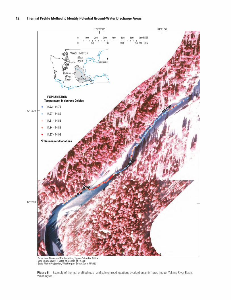
Several other methods are available to display and analyze profile information. Information input to a GIS can be plotted spatially using the USGS Digital Raster Graphs to display all or part of the profile. Spatially displayed profile data using Digital Ortho-Quadrangles and color infra-red images for the base map also were used for this study. An example of color infra-red images of a map for a short section of a profiled reach is shown in figure 6; this map also shows locations of salmon redds in this spawning reach. Images can show small features (for example, reconnecting side channels), which may help explain temperature variations in the profile. Another method to display the data is to graph temperature changes between readings. Diversity in such a plot is generally represented by similar changes for reasonable distances and structure by large changes over small distances. The spatial plot of such changes also provides valuable insight into the relative spatial variations of temperature changes. Temperature changes also can be accumulated and plotted against either distance or time. Such a plot has the same shape as the actual data, but is in terms of cumulative change in temperature for the profile.
Figure �. Thermal profile and depth for the cooling part of the example reach, August 8, 2001, Yakima River Basin, Washington.
waA4WT1_03_fig05
TemperatureDepth
DEPT
H, IN
CEN
TIM
ETER
S
22.0
22.5
23.0
23.5
16 17 18 19 20 21 22 230
100
200
300
400
TEM
PERA
TURE
, IN
DEG
REES
CEL
SIUS
DISTANCE, IN KILOMETERS
Example of Method Application 11
waA4WT1_03_fig06
121°01'40" 121°01'30"
47°12'20"
47°12'30"
0
0
200 300
10050 200 METERS150
100 500 600 700 FEET400
Salmon redd locations
Temperature, in degrees CelsiusEXPLANATION
14.72 - 14.76
14.77 - 14.80
14.81 - 14.83
14.84 - 14.86
14.87 - 14.93
Base from Bureau of Reclamation, Upper Columbia OfficeMap images Nov. 1, 2000, at a scale of 1:4,800 State Plane Projection, Washington South Zone, NAD83
WASHINGTON
YakimaRiverBasin
Seattle Spokane
Maparea
Columbia
River
Sn
ake River
Columbia
Riv
er
Yakima
Figure �. Example of thermal profiled reach and salmon redd locations overlaid on an infrared image, Yakima River Basin, Washington.
1� Thermal Profile Method to Identify Potential Ground-Water Discharge Areas
Summary and ConclusionsThe thermal profile method developed for long river
reaches proved to be robust, reliable, and reproducible and can be applied while drifting in a Lagrangian framework, wading, and by using motorized watercraft. Motorized watercraft are best used in quiescent waters such as lakes or boat accessible, non-braided stream reaches. The CTD-Diver™ probe and its container functioned excellently under adverse conditions—typified by large temperature variations (reach temperatures varied from about 2 to 24°C), and continual contact and impact with the streambed. Under both 1- and 3-second sample rates, the CTD-Diver™ probe’s storage was not exceeded and the response of multiple sensors was good. Streaming of spatial coordinates using a Global Positioning System (GPS) connected to a laptop computer also functioned well, as did the self-contained GPS. Considering that the terrain varied greatly over the study reaches and included canyon type areas and heavily forested stream banks in more headwater areas, the loss of GPS reception did not occur as often as may be expected. Reception loss occurred less than 5 percent of the time; however, it can be problematic. The method’s advantages and cost-effectiveness outweighs its limitations.
Profiles for the example reach (1) display much intra-profile diversity and structure; (2) indicate that the diversity and structure measurements are reproducible; and (3) identify ground-water discharge areas. Minimum ground-water discharge values were estimated for a broad area. These values were conservatively estimated to range from about 6 to 9 percent of measured upstream discharge, and under the assumption of equilibrium temperature, they are within the range of error in the discharge value from the streamflow measuring station at the upstream end of the reach. The method is able to locate ground-water discharge areas that may not be identifiable from discharge measurements. These ground-water discharge areas were located using deviations from the diurnal heating. In the thermal profile, broad discharge areas are typified by stabilization, cooling, or declining rate of change in temperature increases. Local discharge is exhibited as structure (short temporal variations) contained in the thermal profile. Some local discharge areas were not only small, but were identified based on minor water temperature changes while drifting at high velocities (1.2–1.8 meters per second).
Thermal processes leading to end-member temperatures of a reach could not have been identified using available techniques. Realistic thermal modeling of these reaches would be time-consuming and would not provide details of the thermal habitat information contained in the profiles.
For habitat assessment, thermal profiles delineate the thermal habitat at a small scale. When combined with detailed pool-riffle-run structure documented in the depth data, a clearer picture of habitat for salmonids can be obtained. Profiling of many reaches and inclusion of fish survey data can
potentially lead to an improved understanding of the relation between the different life-history stages of salmonids and the thermal-depth habitat in a basin.
Although this method does not supplant other methods, it is a cost-effective way to enhance analysis and use of data gathered using other techniques. Thermal-depth profiling of headwater and first to second order streams was not tested. In many areas in the western United States, these parts of streams represent the only remaining patches of suitable habitat for some salmonids (Rieman and Dunham, 2000). Determining whether this method can be applied in these areas would be beneficial, because terrain may disallow GPS reception. This leads to the question of the value of a thermal-depth profile for a reach that is not tied in with spatial coordinates, especially because temperature is thought to be a limiting factor for most life-history stages of salmonids in many river basins. Without spatial coordinates, a thermal profile completed between two fixed stations may well provide valuable information on the response of a water parcel as it moves downstream in these environments. Thus, providing a better estimate of the value of the fixed station data relative to processes occurring along a reach.
A thermal profile provides valuable information on spatial and temporal variations in the thermal regime and habitat, indicates ground-water discharge areas, and identifies areas for more detailed study. Thermal profiles display diversity and structure that can not be captured by fixed station data.
References CitedAlderdice, D.F., and Velsen, F.P., 1978, Relation between
temperature and incubation time for eggs of chinook salmon Oncorhynchus tshawytscha: Journal of Fisheries Research Board of Canada, v. 35, p. 69-75.
Anderson, E.R., 1954, Energy-budget studies, Lake Hefner Studies, Technical Report: U.S. Geological Survey Professional Paper 269, p. 71-119.
Bencala, K.E., and Walters, R.A., 1983, Simulation of solute transport in a mountain pool-and-riffle stream: A transient storage model: Water Resources Research, v. 19, p. 718-724.
Benson, N.B., 1953, The importance of groundwater to trout populations in the Pigeon River, Michigan: Transactions of the North American Wildlife Conference, 18: p. 269-281.
Berman, C.H., and Quinn, T.P., 1991, Behavioral thermoregulation and homing by spring chinook salmon, Oncorhynchus tshawytscha (Walbaum), in the Yakima River: Journal of Fish Biology, v. 39, p. 301-312.
Beschta, R.L., Bilby, R.E., Brown, G.W., Holtby, L.B., and Hofstra, T.D., 1987, Stream temperatures and aquatic habitat: Fisheries and forest interaction, E.O. Salo and T.W. Cundy, eds.: Proceedings of symposium, February 1986, University of Washington, Seattle, Wash., p. 191-232.
References Cited 1�
Brett, J.R., 1956, Some principles in the thermal requirements of fishes: Quarterly Review of Biology, v. 31, No. 2, p. 75-87.
Brown, R.S., and Mackay, W.C., 1995, Fall and winter movements of and habitat use by cutthroat trout in the Ram River, Alberta: Transactions of American Fisheries Society, v. 124, p. 873-885.
Brunke, M., and Gonser, T., 1997, The ecological significance of exchange processes between rivers and groundwater: Freshwater Biology, v. 37, p 1-33.
Burrows, R.E., 1963, Water temperature requirements for maximum productivity of salmon, in Water temperature influences, effects, and control: Corvallis, Oreg., 12th Pacific Northwest Conference on Water Pollution Research Proceedings, Pacific Northwest National Laboratory, p. 29-38.
Cartwright, Keros, 1970, Groundwater discharge in the Illinois basin as suggested by temperature anomalies: Water Resources Research, v. 6, No. 3, p. 912-918.
Coble, D.W., 1961, Influence of water exchange and dissolved oxygen in redds on the survival of steelhead trout embryos: Transactions of American Fisheries Society, vol.. 90, p. 469-474.
Combs, B.D., 1965, Effects of temperature on the development of salmon eggs: Progressive Fish-Culture, v. 27, p. 134-137.
Combs, B.D., and Burrows, R.E., 1957, Threshold temperatures for the normal development of Chinook salmon eggs: Progressive Fish-Culture, v. 19, p. 3-6.
Constanz, Jim, 1998, Interaction between stream temperature, streamflow, and groundwater exchanges in alpine streams: Water Resources Research, v. 34, No. 7, p. 1609-1615.
Constanz, Jim, Stonestrom, David, Stewart, A.E., Niswonger, Richard, and Smith, T.R., 2001, Analysis of streambed temperatures in ephemeral channels to determine streamflow frequency and duration: Water Resources Research, v. 37, no. 2, p. 317-328.
Curry, R.A., Noakes, D.L., and Morgan, G.E., 1995, Groundwater and the incubation and emergence of brook trout (Salelinus fontinalis): Canadian Journal of Fisheries and Aquatic Science, v. 52, p. 1741-1749.
Eaton, J.G., McCormick, B.E., Goodno, B.E., Stefan, H. H., and Scheller, R.M., 1995, A field information-based system for estimating fish temperature tolerances: Fisheries, v. 20, No. 4, p. 10-18.
Edinger, J.E., Duttweiler, D.W., and Geyer, J.C., 1968, The response of water temperatures to meteorological conditions: Water Resources Research, v. 4, No. 5, p. 1137-1143.
Edinger, J.E. and Geyer, J.C., 1968, Analyzing stream electric power plant discharges: American Society of Civil Engineers, Journal of Sanitary Engineering, v. 94, No. SA4, p. 611-623.
Fokkens, B., and Weijenberg, J., 1968, Measuring the hydraulic potential of groundwater with the hydraulic potential probe: Journal of Hydrology, v. 6, p. 306-313.
Gangmark, H.A., and Bakkala, R.G., 1958, Plastic standpipe for sampling streambed environment of salmon species: U.S. Fish and Wildlife Service, Special Scientific Report-Fisheries, no. 261, 21 p.
Gregory, J.S., and Griffith, J.L., 1996, Aggressive behavior of underyearling rainbow trout in simulated winter concealment habitat: Journal of Fisheries Biology, v. 49, p. 237-245.
Harbeck, G.E., Koberg, G.E., and Hughes, G.H., 1959, The effect of the addition of heat from a power plant on the thermal structure and evaporation of Lake Colorado City, Tex.: U.S. Geological Survey Professional Paper 272-B.
Harvey, F.E., Lee, D.R., Rudolph, D.L., and Frape, S.K., 1997, Locating groundwater discharge in large lakes using bottom sediment electrical conductivity mapping: Water Resources Research, v. 33, no. 11, p. 2609-2615.
Harvey, J.W., and Wagner, B.J., 2000, Quantifying hydrologic interactions between streams and their subsurface hyporheic zones: in J.A. Jones and P.J. Mulholland, eds.: Streams and Ground Waters, Academic Press, San Diego, Calif., p. 3-44.
Haslam, S., 1978, River plants: The macrophytic vegetation of watercourses: Cambridge University Press, Cambridge, United Kingdom, 396 p.
Hynes, H.B., 1983, Groundwater and stream ecology: Hydrobiologia, vol. 100, p. 93-99
Jackman, A.P., Triska, F.J., and Duff, J.H., 1997, Hydrologic examination of ground-water discharge into the upper Shingobee River: U.S. Geological Survey Water-Resources Investigations Report 96-4215, p. 137-142.
Jackman, A.P., Walters, R.A., and Kennedy, V.C., 1984, Transport and concentration controls for chloride, strontium, potassium and lead in Uvas Creek, a small cobble-bed stream in Santa Clara County, California, USA—2. Mathematical modeling: Journal of Hydrology, v. 75, p. 111-141.
Jobling, M., 1981, Temperature tolerance and the final preferendum-rapid methods for the assessment of optimum growth temperatures: Journal of Fish Biology, v. 19, p. 439-455.
Jobson, H.E., 1977, Bed conduction computation for thermal models: American Society of Civil Engineers, Journal of Hydraulics Division, v. 103, no. HY10, p. 1217-1221.
Keller, E.A., Hofstra, T.D., and Moses, Clarice, 1996, Summer cold pools in Redwood Creek near Orick, California, and their relation to anadromous fish habitat: in K.M. Nolan, H.M. Kelsey, D.C. Marron, eds.: Geomorphic processes and aquatic habitat in the Redwood Creek Basin, northwestern California: U.S. Geological Survey Professional Paper 1454, p. U1-U9.
Kilpatrick, F.A., and Cobb, E.D., 1985, Measurement of discharge using tracers: U.S. Geological Survey Techniques of Water Resources Investigations, book 3, chap. A16, 26 p.
Koberg, G.E., 1964, Methods to compute long-wave radiation from the atmosphere and reflected solar radiation from a water surface: U.S. Geological Survey Professional Paper 272-F, p 107-136.
1� Thermal Profile Method to Identify Potential Ground-Water Discharge Areas
Lapham, W.W., 1989, Use of temperature profiles beneath streams to determine rates of vertical ground-water flow and vertical hydraulic conductivity: U.S. Geological Survey Water Supply Paper 2337, 35 p.
Lee, D.R., 1977, A device for measuring seepage flux in lakes and estuaries: Limnology and Oceanography, v. 22, p. 155-163.
Lee, D.R., 1985, Method for locating sediment anomalies in lakebeds that can be caused by groundwater flow: Journal of Hydrology, v. 79, p. 187-193.
Lee, D.R., and Cherry, J.A., 1978, A field exercise on groundwater flow using seepage meters and mini-piezometers: Journal of Geological Education, v. 27, p. 6-10.
Lee, D.R., and Dal Bianco, R., 1994, Methodology for locating and quantifying acid mine drainage in ground waters entering surface waters: Proceedings of the International Land Reclamation and Mine Drainage Conference and the Third International Conference on the Abatement of Acidic Drainage, Pittsburgh, Pa., April 24-29, 1994, Special Publication SP06-A94, vol. 1: Bureau of Mines, U.S. Department of the Interior, p. 327-335.
Lee, D.R., and Hynes, H.B., 1978, Identification of groundwater discharge zones in a reach of Hillman Creek in southern Ontario: Water Pollution Research in Canada, v. 13, p. 121-133.
Lee, D.R., Geist, D.R., Saldi, Kay, Hartwig, Dale, and Cooper, Tom, 1997, Locating ground-water discharge in the Hanford Reach of the Columbia River: Report RC-M-22, PNNL-11516, Atomic Energy of Canada Ltd., Pacific Northwest National Laboratory, AECL, Chalk River, Ontario, Canada, 37 p.
Magnuson, J.J., Crowder, L.B., and Medvick, P.A., 1979, Temperature as an ecological resource: American Zoologist, v. 19, p. 331-343.
Messinger, H., 1963, Dissipation of heat from a thermally loaded stream: U.S. Geological Survey Professional Paper 475-C, 177 p.
Modica, E., Reilly, T.E., and Pollock, D.W., 1997, Patterns and age distribution of ground-water flow to streams: Ground Water, v. 35, no. 3, p. 523-537.
Poff, N.L., and Ward, J.V., 1990, The physical habitat template of lotic systems: recovery in the context of historical pattern of spatio-temporal heterogeneity: Environmental. Management, v. 14, p. 629-646.
Power, G., Brown, R.S., and Imhof, J.G, 1999, Groundwater and fish-insights from North America: Hydrologic Process, v. 13, p. 401-422.
Raphael, J.M., 1962, Prediction of temperature in rivers and reservoirs: American Society of Civil Engineers., Journal Power Division, v. 88, no. PO2, p. 157-181.
Reeves, G.H., Hall, J.D., Roelofs, T.D., Hickman, T.L., and Baker, C.O., 1991, Rehabilitating and modifying stream habitats: American Fisheries Society Special Publication, v. 19, p. 519-558.
Rieman, B.E., and Dunham, J.B, 2000, Metapopulations and salmonids: a synthesis of life history patterns and empirical observations: Ecology of Freshwater Fishes, v. 9, p. 51-64.
Silliman, S.E., and Booth, D.F., 1993, Analysis of time-series measurements of sediment temperatures for identification of gaining vs. losing portions of Juday Creek, Indiana: Journal of Hydrology, v. 146, p. 131-148.
Simonds, F.W., Longpre, C.I., and Justin, G.B., 2004, Ground-water system in the Chimacum Creek Basin and Surface water/ground water interaction in Chimacum and Tarboo Creeks and the Big and Little Quilcene Rivers, eastern Jefferson County: U.S. Geological Survey Scientific Investigations Report 2004-5058, 49 p.
Sinokrot, B.A., and Stefan, H.G., 1993, Stream temperature dynamics: Measurement and modeling: Water Resources Research, v. 29, no. 7, p. 2299-2313.
Southwood, T.R.E., 1977, Habitat, the templet for ecological strategies?: Journal of Animal Ecology, v. 46, p. 337-365.
Sowden, T.K., and Power, G., 1985, Prediction of rainbow trout embryo survival in relation to groundwater seepage and particle size of spawning substrates: Transactions of American Fisheries Society, v. 11, p. 804-812.
Stanford, J.A., and Simons, J.J., eds., 1992, Proceedings of the First International Conference on Ground Water Ecology: American Water Resources Association, TPS-92-92, Bethesda, Md., 420 p.
Stanford, J.A., and Ward, J.V., 1993, An ecosystem perspective of alluvial rivers: connectivity and the hyporheic corridor: Journal of North American Benthological Society, v. 12, no. 1, p. 48-60.
Stevens, H.H., Ficke, J.F., and Smoot, G.F., 1975, Water temperature-influential factors, field measurement, and data presentation: U.S. Geological Survey Techniques of Water-Resources Investigations, book 1, chap. D1, 65 p.
Systems Operations Advisory Committee, 1999, Report on biologically based flows for the Yakima River Basin: Report to The Secretary of the Interior, May 1999, Yakima, Wash., Executive Summary, 6 chap., 1 app.
Terhune, L.D., 1958, The Mark VI groundwater standpipe for measuring seepage through salmon spawning gravels: Journal of Fisheries Research Board of Canada, v. 15, no. 5, p. 1027-1063.
Triska, F.J., Kennedy, V.C., Avanzino, R.J., Zellweger, G.W., and Bencala, K.E., 1989, Retention and transport of nutrients in a third-order stream in Northwestern California: Hyporheic processes: Ecology, v. 70, p. 1893-1905.
Vannote, R.L., Minshall, G.W., Cummins, K.W., Sedell, J.R., and Cushing, C.E., 1980, The river continuum concept: Canadian Journal of Fisheries and Aquatic Science, v. 37, p. 130-137.
Vannote, R.L., and Sweeney, B.W., 1980, Geographic analysis of thermal equilibria: A conceptual model for evaluating the effect of natural and modified thermal regimes on aquatic insect communities: The American Naturalist, v. 115, no. 5, P. 667-695.
References Cited 1�
Vaux, W.F., 1962, Interchange of stream and intragravel water in a salmon spawning riffle: U.S. Fish and Wildlife Service, Special Scientific Report-Fisheries, no. 405, 11 p.
Wetzel, R.G., 1990, Land-Water Interfaces: Metabolic and limnological regulators: Verh. Internationale Vereinigun. Limnologie, v. 24, p. 6-24.
White, D.S., Elzinga, C.H., and Hendricks, S.P., 1987, Temperature patterns within the hyporheic zone of a northern Michigan river: Journal of North American Benthological Society, v. 6, p. 85-91.
Winter, T.C., Harvey, J.W., Franke O.L., and Alley, W.M., 1998, Ground water and surface water: a single resource: U.S. Geological Survey Circular 1139, 79 p
Winter, T.C., LaBaugh, J.W., and Rosenberry, D.O., 1988, The design and use of a hydraulic potentiometer for direct measurement of differences in hydraulic head between groundwater and surface water: Limnology and Oceanography, v. 33, p 1209-1214.
Woessner, W.W., and Brick, Christine, 1992, The role of groundwater in sustaining shoreline spawning kokanne salmon, Flathead Lake, Montana: in J.A. Stanford, and J.J. Simons, eds., Proceedings of the First International Conference on Ground Water Ecology: American Water Resources Association, TPS-92-92, Bethesda, Md., p. 257-266.
1� Thermal Profile Method to Identify Potential Ground-Water Discharge Areas
Manuscript approved for publication, June 13, 2006Prepared by the Publishing Network, Publishing Service Center, Tacoma, Washington
Bill Gibbs Bob Crist Debra Grillo Donita Parker Sharon Wahlstrom
For more information concerning the research in this report, contact the Washington Water Science Center Director U.S. Geological Survey 934 Broadway, Suite 300 Tacoma, Washington 98402 http://wa.water.usgs.gov