A thermodynamic model for estimating sea and lake ice thickness with optical satellite data Xuanji Wang, 1 Jeffrey R. Key, 2 and Yinghui Liu 1 Received 30 September 2009; revised 4 August 2010; accepted 13 September 2010; published 16 December 2010. [1] Sea ice is a very important indicator and an effective modulator of regional and global climate change. Current remote sensing techniques provide an unprecedented opportunity to monitor the cryosphere routinely with relatively high spatial and temporal resolutions. In this paper, we introduce a thermodynamic model to estimate sea and lake ice thickness with optical (visible, nearinfrared, and infrared) satellite data. Comparisons of nighttime ice thickness retrievals to ice thickness measurements from upward looking submarine sonar show that this thermodynamic model is capable of retrieving ice thickness up to 2.8 m. The mean absolute error is 0.18 m for samples with a mean ice thickness of 1.62 m, i.e., an 11% mean absolute error. Comparisons with in situ Canadian stations and moored upward looking sonar measurements show similar results. Sensitivity studies indicate that the largest errors come from uncertainties in surface albedo and downward solar radiation flux estimates from satellite data, followed by uncertainties in snow depth and cloud fractional coverage. Due to the relatively large uncertainties in current satellite retrievals of surface albedo and surface downward shortwave radiation flux, the current model is not recommended for use with daytime data. For nighttime data, the model is capable of resolving regional and seasonal variations in ice thickness and is useful for climatological analysis. Citation: Wang, X., J. R. Key, and Y. Liu (2010), A thermodynamic model for estimating sea and lake ice thickness with optical satellite data, J. Geophys. Res., 115, C12035, doi:10.1029/2009JC005857. 1. Introduction [2] Changes in sea ice significantly affect the exchanges of momentum, heat, and mass between the sea and the atmosphere. While sea ice extent is an important indicator and effective modulator of regional and global climate change, sea ice thickness is the more important parameter from a thermodynamic perspective. [3] There are some ice thickness data from submarine UpwardLooking Sonar (ULS) during various field cam- paigns, for instance, the Scientific Ice Expeditions (SCICEX) in 1996, 1997, and 1999 [ National Snow and Ice Data Center, 2006]. There are some in situ measurements of ice thickness from the New Arctic Program initiated by the Canadian Ice Service (CIS) starting in 2002, and sea ice draft measurements from moored ULS instruments in the Beaufort Gyre Observing System (BGOS). There are a few studies on changes in sea ice thickness and volume, but they are for specific locations over a limited time period, such as the work by Rothrock et al. [2008] using the ice draft pro- files from submarine transects. The amount of available ice thickness data is insufficient for most largescale studies. [4] Many numerical oceansea iceatmosphere models can, to large extent, simulate sea ice extent with sufficient accuracy to capture its spatial and temporal distributions, as demonstrated by the Intergovernmental Panel on Climate Change Fourth Assessment Report (IPCC AR4) models [Zhang and Walsh, 2006]. Only can few numerical oceansea iceatmosphere models simulate ice thickness distribu- tion, notably, the PanArctic IceOcean Modeling and Assimilation System (PIOMAS) developed by Zhang and Rothrock [2003]. All the model simulations have relatively low spatial resolution compared to satellite data. [5] Accurate, consistent ice thickness data with high spatial resolution are critical for a wide range of applications including climate change detection, climate modeling, and operational applications such as shipping and hazard miti- gation. Satellite data provide an unprecedented opportunity to monitor the cryosphere routinely with relatively high spatial and temporal resolutions for both sea ice, and lake and river ice. [6] Spaceborne sensors, particularly passive microwave radiometers and synthetic aperture radar, have been used primarily to map ice extent and ice concentration, and to monitor and study their trends [Comiso, 2002; Francis et al., 2009; Francis and Hunter, 2007; Maslanik et al., 2007; Drobot et al., 2008]. Some sea ice thickness data have been estimated from satellite radar altimetry since 1993 [Laxon et al., 2003], and will be estimated in the future from the recently launched European Space Agency (ESA) CryoSat2 1 Cooperative Institute of Meteorological Satellite Studies, University of Wisconsin–Madison, Madison, Wisconsin, USA. 2 NESDIS, NOAA, Madison, Wisconsin, USA. Copyright 2010 by the American Geophysical Union. 01480227/10/2009JC005857 JOURNAL OF GEOPHYSICAL RESEARCH, VOL. 115, C12035, doi:10.1029/2009JC005857, 2010 C12035 1 of 14
Transcript
A thermodynamic model for estimating sea and lake icethickness with optical satellite data
Xuanji Wang,1 Jeffrey R. Key,2 and Yinghui Liu1
Received 30 September 2009; revised 4 August 2010; accepted 13 September 2010; published 16 December 2010.
[1] Sea ice is a very important indicator and an effective modulator of regional and globalclimate change. Current remote sensing techniques provide an unprecedented opportunityto monitor the cryosphere routinely with relatively high spatial and temporal resolutions.In this paper, we introduce a thermodynamic model to estimate sea and lake ice thicknesswith optical (visible, near!infrared, and infrared) satellite data. Comparisons of nighttime icethickness retrievals to ice thickness measurements from upward looking submarine sonarshow that this thermodynamic model is capable of retrieving ice thickness up to 2.8 m. Themean absolute error is 0.18 m for samples with a mean ice thickness of 1.62 m, i.e., an 11%mean absolute error. Comparisons with in situ Canadian stations and moored upwardlooking sonar measurements show similar results. Sensitivity studies indicate that the largesterrors come from uncertainties in surface albedo and downward solar radiation fluxestimates from satellite data, followed by uncertainties in snow depth and cloud fractionalcoverage. Due to the relatively large uncertainties in current satellite retrievals of surfacealbedo and surface downward shortwave radiation flux, the current model is notrecommended for use with daytime data. For nighttime data, the model is capable ofresolving regional and seasonal variations in ice thickness and is useful for climatologicalanalysis.
Citation: Wang, X., J. R. Key, and Y. Liu (2010), A thermodynamic model for estimating sea and lake icethickness with optical satellite data, J. Geophys. Res., 115, C12035, doi:10.1029/2009JC005857.
1. Introduction
[2] Changes in sea ice significantly affect the exchangesof momentum, heat, and mass between the sea and theatmosphere. While sea ice extent is an important indicatorand effective modulator of regional and global climatechange, sea ice thickness is the more important parameterfrom a thermodynamic perspective.[3] There are some ice thickness data from submarine
Upward!Looking Sonar (ULS) during various field cam-paigns, for instance, the Scientific Ice Expeditions (SCICEX)in 1996, 1997, and 1999 [National Snow and Ice DataCenter, 2006]. There are some in situ measurements of icethickness from the New Arctic Program initiated by theCanadian Ice Service (CIS) starting in 2002, and sea icedraft measurements from moored ULS instruments in theBeaufort Gyre Observing System (BGOS). There are a fewstudies on changes in sea ice thickness and volume, but theyare for specific locations over a limited time period, such asthe work by Rothrock et al. [2008] using the ice draft pro-files from submarine transects. The amount of available icethickness data is insufficient for most large!scale studies.
[4] Many numerical ocean!sea ice!atmosphere modelscan, to large extent, simulate sea ice extent with sufficientaccuracy to capture its spatial and temporal distributions, asdemonstrated by the Intergovernmental Panel on ClimateChange Fourth Assessment Report (IPCC AR4) models[Zhang and Walsh, 2006]. Only can few numerical ocean!sea ice!atmosphere models simulate ice thickness distribu-tion, notably, the Pan!Arctic Ice!Ocean Modeling andAssimilation System (PIOMAS) developed by Zhang andRothrock [2003]. All the model simulations have relativelylow spatial resolution compared to satellite data.[5] Accurate, consistent ice thickness data with high
spatial resolution are critical for a wide range of applicationsincluding climate change detection, climate modeling, andoperational applications such as shipping and hazard miti-gation. Satellite data provide an unprecedented opportunityto monitor the cryosphere routinely with relatively highspatial and temporal resolutions for both sea ice, and lakeand river ice.[6] Spaceborne sensors, particularly passive microwave
radiometers and synthetic aperture radar, have been usedprimarily to map ice extent and ice concentration, and tomonitor and study their trends [Comiso, 2002; Francis et al.,2009; Francis and Hunter, 2007; Maslanik et al., 2007;Drobot et al., 2008]. Some sea ice thickness data have beenestimated from satellite radar altimetry since 1993 [Laxonet al., 2003], and will be estimated in the future from therecently launched European Space Agency (ESA) CryoSat!2
1Cooperative Institute of Meteorological Satellite Studies, University ofWisconsin–Madison, Madison, Wisconsin, USA.
2NESDIS, NOAA, Madison, Wisconsin, USA.
Copyright 2010 by the American Geophysical Union.0148!0227/10/2009JC005857
JOURNAL OF GEOPHYSICAL RESEARCH, VOL. 115, C12035, doi:10.1029/2009JC005857, 2010
mission (http://www.esa.int/esaLP/ESAOMH1VMOC_LPcryosat_0.html). With the launch of the ICESat satellitein January of 2003, sea ice thickness and volume estimationmethods were developed for use with elevation data fromICESat’s laser altimeter [Kwok and Cunningham, 2008;Kwok et al., 2009; Zwally et al., 2008].[7] Can the longer!term records of optical (visible,
near!infrared, infrared) satellite data onboard polar orbitingsatellites be used to retrieve ice thickness? Since the firstlaunch of the U.S. National Oceanic and AtmosphericAdministration (NOAA) Television and InfraRed Observa-tion Satellite (TIROS) series in 1962, the Advanced VeryHigh Resolution Radiometer (AVHRR) has been widelyused in many geophysical applications including the map-ping of ice extent. Can optical satellite imagers such as theAVHRR and Moderate Resolution Imaging Spectro-radiometer (MODIS) also be used to estimate ice thickness?Some work has been done in this field [cf. Yu and Rothrock,1996]. However, those studies have been limited to casestudies of thin ice.[8] This paper presents a model based on ice surface
energy budget to estimate sea and lake ice thickness withoptical satellite data. This model is capable of deriving icethickness up to 2.8 m under both clear! and cloudy!skyconditions with accuracy of greater than 80%. This paper isorganized as follows. Section 2 describes the physics of themodel with its three components: radiative, turbulent, andconductive fluxes. Applications of the model using differentsatellite data for ice thickness retrievals are given in section3. Section 4 presents validation results of ice thickness re-trievals using this model with submarine, station, andmooring data in the Arctic. Quantitative analysis of theuncertainties and sensitivities of our model is discussed insection 5. Discussion and conclusions follow in section 6.
2. One!Dimensional Thermodynamic Ice Model
[9] A slab model proposed by Maykut and Untersteiner[1971] is used here as the basis for our One!dimensionalThermodynamic Ice Model (OTIM). The general equationfor energy conservation at the surface (ice or snow) is
1! !s" #Fr ! I0 ! Fupl $ Fdn
l $ Fs $ Fe $ Fc % Fa "1#
where as is the ice or snow covered surface shortwavebroadband albedo, Fr is the downward shortwave radiationflux at the surface, I0 is the shortwave radiation flux passingthrough the ice interior with ice slab transmittance i0, Fl
up isthe upward longwave radiation flux from the surface, Fl
dn isthe surface downward longwave radiation flux from theatmosphere, Fs is the sensible heat flux at the surface, Fe isthe latent heat flux at the surface, Fc is the conductive heatflux within the ice slab, and Fa is the residual heat flux thatcould be caused by ice melting and/or heat horizontaladvection. Flux entering the surface is positive, and fluxleaving the surface is negative. By definition, in equation (1),as, Fr, I0, Fl
up, Fldn should be always positive, Fs, Fe, and Fc
could be positive or negative, and Fa is usually assumed to bezero in the absence of a phase change. The details of each termwill be addressed in sections 2.1 through 2.7.
2.1. Shortwave Radiation at the Surface and Throughthe Ice[10] The first term on the left!hand side of equation (1),
(1 ! as) Fr, is the net shortwave radiation flux at the surface.The surface broadband albedo over entire solar spectrum, as,is estimated [Grenfell, 1979] by
!s % 1! A exp !Bh" # ! C exp !Dh" # "2#
where A, B,C, andD are empirically derived coefficients, andh is the ice thickness (hi) or snow depth (hs) in meter if snow ispresent over the ice. The other relatively simple approaches todetermine ice and snow surface albedo include model simu-lated constant values based on the ice and snow types asdiscussed by Saloranta [2000], and the experimental andobservational values for a variety of snow and ice surfaceconditions as discussed by Grenfell and Perovich [2004].Equation (2) is chosen for surface albedo estimation is basedon the following considerations. (1) It is not constant but afunction of ice thickness, ice type, and snow depth. (2) Thecoefficients A, B, C, and D are dependent on ice types andsnow depth, and different for clear! and cloudy!sky condi-tions that make it suitable for use with satellite data. (3) It isrelatively easy to improve the broadband albedo estimationby adjusting A, B, C, and D values accordingly with moreupdated validation results. The values of A, B, C, and D aregiven by Grenfell [1979, Table 1]. The downward shortwaveradiation flux at the surface, Fr, can be either an inputparameter or parameterized with parameterization schemesbuilt into the OTIM. There are a number of parameterizationschemes estimating Fr under both clear! and cloudy!skyconditions for cold regions. Key et al. [1996] compared theseschemes for applications in high latitude, including clear!skyparameterization schemes from Shine and Henderson!Sellers[1985], Moritz [1978], and Bennett [1982], and cloudy!skyparameterization schemes from Shine [1984],Bennett [1982],Jacobs [1978], Laevastu [1960], and Berliand [1960]. Forclear! and cloudy!sky downward shortwave radiation fluxesin the OTIM, the Shine [1984] schemes are used.[11] The second term on the left!hand side of equation (1),
I0 = i0 (1 ! as)Fr, is the shortwave radiation flux passingthrough the ice interior. i0 is the ice slab transmittance, i.e.,the percentage of the shortwave radiation flux that pene-trates the ice, which is estimated by the following parame-terization scheme by Grenfell [1979]:
i0 % A exp !Bh" # $ C exp !Dh" # "3#
where A, B, C, and D are coefficients that are different fromthose in equation (2), and h is the ice slab thickness inmeters.
2.2. Longwave Radiation at the Surface[12] The third term on the left!hand side of equation (1),
Flup, is the upward longwave radiation flux from the surface
to the atmosphere, which is estimated with
Fupl % ""T4
s "4#
where " is the longwave emissivity of the ice or snow sur-face, s is the Stefan!Boltzman constant, and Ts is the surface
WANG ET AL.: ICE THICKNESS MODEL C12035C12035
2 of 14
skin temperature in K. For simplicity, an ice emissivity of0.988 is used. Even though some pixels contain a smallportion of open water or snow, the error in emissivity fromimproperly defining the surface type is small because snowemissivity at a 0 degree look angle is 0.995, very close tothe value of 0.987 for ice and 0.988 for water [Rees,1993].[13] The fourth term on the left!hand side of equation (1),
Fldn, is the surface downward longwave radiation flux from
the atmosphere. There are five potential clear!sky parame-terization schemes for estimating the downward longwaveradiation flux: Yu and Rothrock [1996], Efimova [1961],Ohmura [1981], Maykut and Church [1973], and Andreasand Ackley [1982]. There are also five potential cloudy!sky parameterization schemes: Yu and Rothrock [1996],Jacobs [1978], Maykut and Church [1973], Zillman [1972],and Schmetz and Raschke [1986]. Based on the Key et al.[1996] study, the Efimova [1961] scheme is the mostaccurate for clear!sky conditions: Fl,clr
dn = s Ta4 (0.746 +
0.0066 ea), where ea is the water vapor pressure (hPa) nearthe surface, and Ta is the air temperature at 2 m above thesurface. For cloudy!sky conditions, the Jacobs [1978]scheme is the best estimator: Fl
dn = Fl,clrdn (1 + 0.26C),
where C is fractional cloud cover. These two schemes areused for estimating the downward longwave radiation fluxat the surface.
2.3. Surface Sensible Heat Flux[14] The fifth term on the left!hand side of equation (1),
Fs, is the surface sensible heat flux, which is calculated byfollowing formula:
Fs % #aCpCsu Ta ! Ts" # "5#
where ra is the air density (standard value of 1.275 kg m!3 at0°C and 1000 hPa), Cp is the specific heat of wet air withwet air specific humidity q, Cs is the bulk transfer coefficientfor sensible heat flux between the air and ice surface (Yu andRothrock [1996] use Cs = 0.003 for very thin ice, and0.00175 for thick ice, 0.0023 for neutral stratification assuggested by Lindsay [1998] in his energy balance modelfor thick Arctic pack ice), u is the surface wind speed, Ta isthe near surface air temperature at 2 m above the ground,and Ts is the surface skin temperature. The wet air density rais calculated using the gas law with surface air pressure Pa inhPa, surface air virtual temperature Tv in K, and the gasconstant Rgas (287.1 J kg!1 K!1) by the formula #a % 100Pa
RgasTv,
where Tv = (1 + 0.608q)Ta and q is the wet air specifichumidity (kg/kg). The wet air specific heat is
Cp % Cpd 1! q$Cpv
Cpdq
! ""6#
where Cpv is the specific heat of water vapor at constantpressure (1952 J K!1 kg!1) and Cpd is the specific heat of dryair at constant pressure (1004.5 J K!1 kg!1), so Cp cansimply be written as Cp = 1004.5 · (1 + 0.9433q). The relativehumidity over the snow/ice is assumed to be 90%, if it isunknown.
2.4. Surface Latent Heat Flux[15] The sixth term on the left!hand side of equation (1),
Fe, is the latent heat flux at the surface. It is calculated in theOTIM with
Fe % #a L Ce u wa ! wsa" # "7#
where ra is the air density, L is the latent heat of vapori-zation (2.5 ! 106 J kg!1) which should include the latentheat fusion/melting (3.34 ! 105 J kg!1) if the surface isbelow freezing, Ce is the bulk transfer coefficient for latentheat flux of evaporation, u is the surface wind speed, wa isthe air mixing ratio at 2 m above the ground, and wsa is themixing ratio at the surface. The mixing ratio is very close tothe specific humidity in magnitude, w = q/(1 ! q) & q.[16] The bulk transfer coefficient, Ce, for the latent heat
flux is a function of wind speed and/or air!sea ice temper-ature difference. It can be parameterized as described byBentamy et al. [2003] and used in this study by the formulaCe = {a exp[b (u + c)] + d/u + 1} ! 10!3, where a =!0.146785, b = !0.292400, c = !2.206648, and d =1.6112292. The Ce value ranges between 0.0015 and 0.0011for wind speeds between 2 and 20 m s!1. Another parame-terization scheme of Ce was developed by Kara et al. [2000]for use in a general circulation model. They related Ce to bothsurface wind speed and air!sea ice temperature difference:
Ce % Ce0 $ Ce1 Ts ! Ta" #
Ce0 % 0:994$ 0:061u! 0:001u2# $
' 10!3
Ce1 % !0:020$ 0:691 1=u" # ! 0:871 1=u" #2h i
' 10!3
where the wind speed is limited to the interval û = max[3.0,min(27.5, u)] to suppress the underestimation of the quadraticfit when u > 27.5 m s!1.[17] Because Cs is so close in value to Ce, a linear rela-
tionship between Ce and Cs is used rather than determiningCs independently. The simplest representative linear for-mulation is found to be Cs = 0.96Ce with a negligibleintercept (3.6 ! 10!6) as reported by Kara et al. [2000]; weuse Cs = 0.98Ce in our model for air!sea ice interface tur-bulent heat transfer.
2.5. Conductive Heat Flux[18] The seventh term on the left!hand side of equation
(1), Fc, is the conductive heat flux for a two!layer systemwith one snow layer over an ice slab that can be written as
Fc % $ Tf ! Ts% &
"8#
where g = (ki ks)/(ks hi + ki hs), Tf is the water freezingtemperature (degrees C) that can be derived from the sim-plified relationship Tf = !0.055Sw, where Sw is the salinity ofseawater, assumed to be 31.0 parts per thousand (ppt) for theBeaufort Sea and 32.5 ppt for the Greenland Sea, hs is thesnow depth, and hi is the ice thickness. ks is the conductivityof snow which can be formulated by ks = 2.845 ! 10!6rsnow2 +2.7 ! 10!4 · 2.0(Tsnow!233)/5 [Ebert and Curry, 1993] that isused in this study, rsnow is the snow density ranging from225 kg m!3 (new snow) to 450 kg m!3 (water!soaked snow),Tsnow is the snow temperature in K. ks can be further sim-
WANG ET AL.: ICE THICKNESS MODEL C12035C12035
3 of 14
plified as ks = 2.22362 ! 10!5.655(rsnow)1.885 [Yen, 1981]. ki isthe conductivity of ice that is estimated by ki = k0 + bSi/(Ti !273) [Untersteiner, 1964] that is adopted in this study, whereb = 0.13 W m!2 kg!1, k0 = 2.22(1 ! 0.00159Ti) W m!1 K!1
that is the conductivity of pure ice [Curry andWebster, 1999].Si is the sea ice salinity and Ti is the temperature within the iceslab. Some experimental relationships between hs and hi, Tiand Ts, Si and hi exist, as described in sections 2.6 and 2.7.[19] It should point out that assuming linear vertical
temperature profile in the ice slab, which means that con-ductive heat flux across the ice slab is uniform, may causeerror in the ice thickness estimation. According to the Zhangand Rothrock’s [2001] simulations, the difference in theannual mean ice thickness of 2.52 m between the three!layermodel with nonlinear vertical temperature profile and thezero!layer model with linear vertical temperature profile is0.07 m, or 3%. Based on their simulations, it is reasonable toassume a linear vertical temperature profile in the ice slab,i.e., conductive heat flux across the ice slab is uniform, inour model for dealing with ice thickness less than 3 m.
2.6. Relationships Between Snow Depth and IceThickness, Surface Temperature and Ice Temperature,and Sea Ice Thickness and Sea Ice Salinity[20] Doronin [1971] used the following relationship to
estimate snow depth as a function of ice thickness, whichwas also used by Yu and Rothrock [1996]:
hs % 0 for hi < 5 cm;
hs % 0:05hi for 5 cm ( hi ( 20 cm;
hs % 0:1hi for hi > 20 cm:
In the real world, snow accumulation over the ice may notfollow the simple relationship above. So if snow depth isavailable, it should be input to the model.[21] The ice temperature Ti is an important factor in the
ice conductivity calculation. It may be significantly differentfrom surface skin temperature that can be measured orretrieved with remote sensed data when there is snow on theice. In general, we can obtain the surface skin temperature Tsfrom satellite with optical data, but not Ti. Yu and Rothrock[1996] suggested that assuming Ti equal to Ts can cause 5%and 1% errors, when ice thickness is 5 cm and 100 cm,respectively. The assumption that the two are equal may bemore valid during the night than the daytime when thesurface heating from the Sun increases the differencebetween the skin (snow) and ice temperatures. Uncertaintyin Ti is one source of errors for the daytime retrieval of icethickness with the OTIM. However, the sensitivity studydescribed later shows that the error in Ti has a smaller effecton the ice thickness derivation than other uncertainties aslike from snow depth and cloud fraction.[22] There are at least three schemes for the relationship
between sea ice thickness hi and sea ice salinity Si. The Coxand Weeks [1974] scheme is
Si % 14:24$ 19:39hi for hi ( 0:4 m;
Si % 7:88$ 1:59hi for hi > 0:4 m:
Jin et al. [1994] gave this relationship:
Si % 7:0! 31:63hi for hi ( 0:3 m;
Si % 8:0! 1:63hi for hi > 0:3 m:
Kovacs [1996] used this scheme:
Si % 4:606$ 0:91603=hi for 0:10 m ( hi ( 2:0 m:
In the OTIM, we use Kovacs’ scheme to express the rela-tionship between sea ice thickness and sea ice salinity.
2.7. Surface Air Temperature[23] Surface air temperature Ta at 2 m height above the
ground is an essential parameter for the OTIM to estimatethe surface downward longwave radiation, sensible, andlatent heat fluxes. Numerical model forecasts generally donot provide good estimates of the surface 2 m air tempera-ture in the polar regions. Thus, if we assume that large!scaleheat sources and sinks, e.g., “hot” leads and cold ice floes,regulate the cold surface 2 m air temperature Ta, therefore Tashould be close to the surface skin temperature Ts overall.Here we assume that
Ta % Ts $ %T "9#
where Ts is the surface skin temperature from satelliteretrievals, and dT is a function of cloud amount. dT is about2.2°C for clear!sky conditions, and reduces to about 0.4°C forovercast sky condition as implied by Persson et al. [2002].Here we set dT = 2.2 ! 1.8Cf, where Cf is the cloud amountranging from 0 to 1.
3. OTIM Applications With Satellite Data
[24] This section describes the applications of the OTIMwith satellite data to estimate ice thickness. While anyoptical satellite data can be used, the applications with datafrom NOAA’s AVHRR and NASA’s MODIS are detailed.Case studies using data from the Spinning Enhanced Visibleand InfraRed Imager (SEVIRI) on the Meteosat SecondGeneration (MSG) satellite, and from the GeostationaryOperational Environmental Satellite (GOES) have also beenperformed, though the results are not presented here.Regardless of the data source, satellite products required byOTIM as inputs are cloud amount, surface skin temperature,surface broadband albedo, and surface downward shortwaveradiation fluxes. The latter two are for daytime retrievalonly.[25] The AVHRR Polar Pathfinder extended (APP!x)
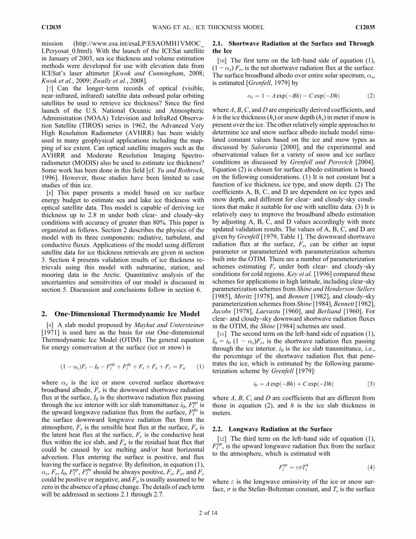
product suite used in this study [Wang and Key, 2003, 2005;Wang et al., 2007; Fowler et al., 2007] can be found with itsproduct description at http://stratus.ssec.wisc.edu/projects/app/app.html. Figure 1 gives an example of the OTIMretrieved sea ice thickness from APP!x data set on 21February 2004 at 04:00am local solar time. For MODISdata, MODIS cloud mask [Ackerman et al., 1998; Liu et al.,2004] and surface skin temperature are used as inputs to theOTIM. The MODIS and AVHRR ice surface skin temper-ature for clear!sky conditions is retrieved using a split!
WANG ET AL.: ICE THICKNESS MODEL C12035C12035
4 of 14
window technique, where split window refers to brightnesstemperature in the 11–12 mm atmospheric window. Theretrieval equation is
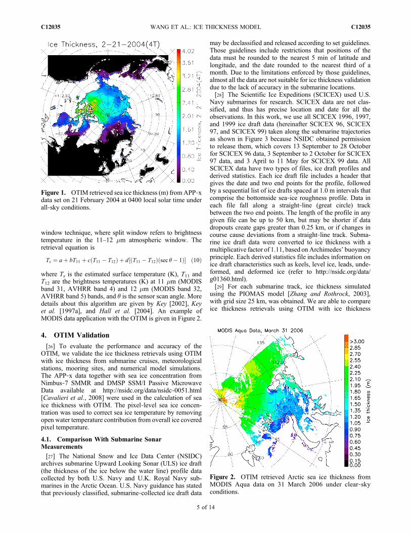
where Ts is the estimated surface temperature (K), T11 andT12 are the brightness temperatures (K) at 11 mm (MODISband 31, AVHRR band 4) and 12 mm (MODIS band 32,AVHRR band 5) bands, and & is the sensor scan angle. Moredetails about this algorithm are given by Key [2002], Keyet al. [1997a], and Hall et al. [2004]. An example ofMODIS data application with the OTIM is given in Figure 2.
4. OTIM Validation
[26] To evaluate the performance and accuracy of theOTIM, we validate the ice thickness retrievals using OTIMwith ice thickness from submarine cruises, meteorologicalstations, mooring sites, and numerical model simulations.The APP!x data together with sea ice concentration fromNimbus!7 SMMR and DMSP SSM/I Passive MicrowaveData available at http://nsidc.org/data/nsidc!0051.html[Cavalieri et al., 2008] were used in the calculation of seaice thickness with OTIM. The pixel!level sea ice concen-tration was used to correct sea ice temperature by removingopen water temperature contribution from overall ice coveredpixel temperature.
4.1. Comparison With Submarine SonarMeasurements[27] The National Snow and Ice Data Center (NSIDC)
archives submarine Upward Looking Sonar (ULS) ice draft(the thickness of the ice below the water line) profile datacollected by both U.S. Navy and U.K. Royal Navy sub-marines in the Arctic Ocean. U.S. Navy guidance has statedthat previously classified, submarine!collected ice draft data
may be declassified and released according to set guidelines.Those guidelines include restrictions that positions of thedata must be rounded to the nearest 5 min of latitude andlongitude, and the date rounded to the nearest third of amonth. Due to the limitations enforced by those guidelines,almost all the data are not suitable for ice thickness validationdue to the lack of accuracy in the submarine locations.[28] The Scientific Ice Expeditions (SCICEX) used U.S.
Navy submarines for research. SCICEX data are not clas-sified, and thus has precise location and date for all theobservations. In this work, we use all SCICEX 1996, 1997,and 1999 ice draft data (hereinafter SCICEX 96, SCICEX97, and SCICEX 99) taken along the submarine trajectoriesas shown in Figure 3 because NSIDC obtained permissionto release them, which covers 13 September to 28 Octoberfor SCICEX 96 data, 3 September to 2 October for SCICEX97 data, and 3 April to 11 May for SCICEX 99 data. AllSCICEX data have two types of files, ice draft profiles andderived statistics. Each ice draft file includes a header thatgives the date and two end points for the profile, followedby a sequential list of ice drafts spaced at 1.0 m intervals thatcomprise the bottomside sea!ice roughness profile. Data ineach file fall along a straight!line (great circle) trackbetween the two end points. The length of the profile in anygiven file can be up to 50 km, but may be shorter if datadropouts create gaps greater than 0.25 km, or if changes incourse cause deviations from a straight!line track. Subma-rine ice draft data were converted to ice thickness with amultiplicative factor of 1.11, based onArchimedes’ buoyancyprinciple. Each derived statistics file includes information onice draft characteristics such as keels, level ice, leads, unde-formed, and deformed ice (refer to http://nsidc.org/data/g01360.html).[29] For each submarine track, ice thickness simulated
using the PIOMAS model [Zhang and Rothrock, 2003],with grid size 25 km, was obtained. We are able to compareice thickness retrievals using OTIM with ice thickness
Figure 2. OTIM retrieved Arctic sea ice thickness fromMODIS Aqua data on 31 March 2006 under clear!skyconditions.
Figure 1. OTIM retrieved sea ice thickness (m) fromAPP!xdata set on 21 February 2004 at 0400 local solar time underall!sky conditions.
WANG ET AL.: ICE THICKNESS MODEL C12035C12035
5 of 14
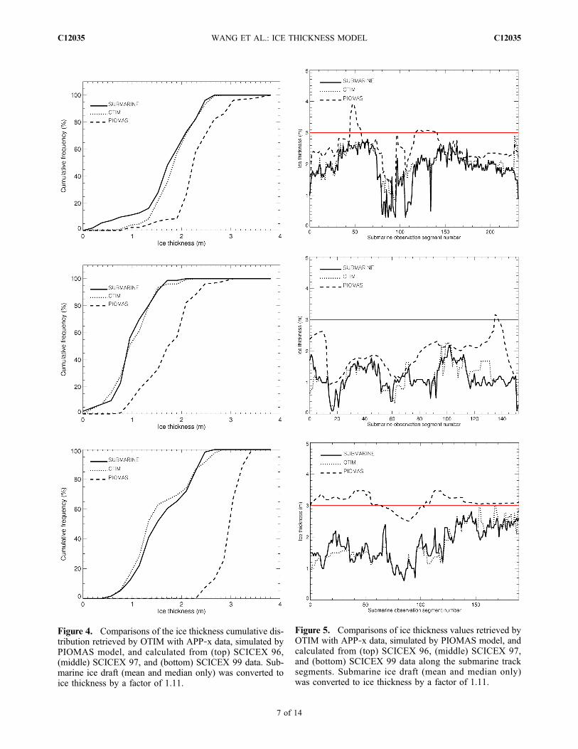
measured by submarines and the corresponding numericalmodel simulations using PIOMAS. Only those submarinetrack segments longer than 25 km are used in this com-parison because the satellite product and numerical modelgrid resolutions are 25 km. For each of the locations ofsubmarine track segments, mooring sites, and metrologicalstations, the nearest valid pixel within a 3 by 3 pixel boxcentered at the location from satellite and numerical modeldata grids on the same date is used for the comparison. If novalid pixel is found within that box from any one of the datasources, in particular, from satellite data grid, the comparisonwill not be done for that date at the location.[30] Figure 4 shows comparisons in cumulative frequency
of sea ice thickness that were retrieved by OTIM with APP!xdata, measured by submarines, and simulated by PIOMASmodel. Figure 5 shows the point!to!point comparisonsamong them. Table 1 lists the comparison results betweenOTIM and submarine measurements. The overall mean icethicknesses are 1.62 m and 1.64 m from all SCICEX data andOTIM retrievals, respectively.[31] The overall mean absolute bias (mean of the absolute
values of the differences) between the OTIM and submarinedata is 0.18 m, or less than 12% error in terms of true meanice thickness. The errors are 16% and 10% for 0.00–1.80 mthick ice and 1.80–3.00 m thick ice, respectively. Manyfactors contribute to the ice thickness differences betweenthe OTIM and submarine data: (1) The actual length of thesubmarine track segments, and the minimum and maximumice draft values from the statistics of the submarine tracksegments. (2) Incorrect cloud identification with satellitedata is one of the error sources of OTIM retrievals alongwith other uncertainties in the retrievals of surface physicalparameters, e.g., surface temperature. (3) The submarinesmade measurements along a line with a particular orienta-tion, while the OTIM retrieved ice thickness is an areaaverage. (4) The designated snow depth of 0.20 m is notapplicable to all submarine track segments.
4.2. Comparison With Canadian MeteorologicalStation Measurements[32] The Canadian Ice Service (CIS) maintains archived
ice thickness and on!ice snow depth measurements forCanadian stations back as far as 1947 for the first establishedstations in the Canadian Arctic (Eureka and Resolute). By thebeginning of 2002 most stations from the original ice thick-ness program had stopped taking measurements. Fortunately,due to an increasing interest in updating this historical data setto support climate change studies, a new program was startedin the fall of 2002, called New Arctic Program (refer to http://ice!glaces.ec.gc.ca/App/WsvPageDsp.cfm?Lang=eng&lnid=5&ScndLvl=no&ID=11703). The stations in thisprogram are listed in Table 2, and their data are used here forOTIM validation.[33] Most of the data in the current archive at the CIS have
been collected by the Atmospheric Environment Program ofEnvironment Canada, and some data are provided by otherorganizations such as the St Lawrence Seaway Authority,Trent University, and Queen’s University. Measurementsare taken at approximately the same location every year on aweekly basis starting after freeze up when the ice is safe towalk on, and continuing until breakup or when the ice be-comes unsafe. Therefore, the measured ice thickness mini-
Figure 3. Submarine trajectories for (top) SCICEX 96,(middle) 97, and (bottom) 99. Data with their starting andending places and dates are marked.
WANG ET AL.: ICE THICKNESS MODEL C12035C12035
6 of 14
Figure 4. Comparisons of the ice thickness cumulative dis-tribution retrieved by OTIM with APP!x data, simulated byPIOMAS model, and calculated from (top) SCICEX 96,(middle) SCICEX 97, and (bottom) SCICEX 99 data. Sub-marine ice draft (mean and median only) was converted toice thickness by a factor of 1.11.
Figure 5. Comparisons of ice thickness values retrieved byOTIM with APP!x data, simulated by PIOMAS model, andcalculated from (top) SCICEX 96, (middle) SCICEX 97,and (bottom) SCICEX 99 data along the submarine tracksegments. Submarine ice draft (mean and median only)was converted to ice thickness by a factor of 1.11.
WANG ET AL.: ICE THICKNESS MODEL C12035C12035
7 of 14
mum is 20 cm for almost all of the stations. The location of theice thickness measurement is selected close to shore, but overa depth of water exceeding the maximum ice thickness. Icethickness is measured to the nearest centimeter using either aspecial auger kit or a hot wire ice thickness gauge. Mea-surements include additional information such as character ofice surface, water features, and method of observations. Thecomparison of the ice thickness between station measure-ments and OTIM retrievals were done the same way asthat between submarine measurements and OTIM retrievalsthat is explained in section 4.1.[34] Figures 6 and 7 show the comparisons of the three
data sets, i.e., OTIM using APP!x with station!measuredsnow depth, PIOMAS simulations, and station measure-ments at Alert, as a cumulative frequency ice thicknessdistribution and as point!to!point comparisons. Table 3gives the statistical results of ice thickness from OTIMand from Canadian stations when both of them have validice thickness data and the stations have valid snow depthdata. The overall error is comparable to the error of OTIMagainst submarine data, i.e., 18%. The differences betweenthe OTIM and stations tend to be large when there is iceridging, rafting, or hummocking at the stations. Besides theerror sources discussed in section 4.1, the differences canalso be caused by other factors, including point versus areameasurements and changing snow conditions over time.
4.3. Comparison With Moored ULS Measurements[35] The Beaufort Gyre Exploration Project (BGEP)
provides ice draft data starting in 2003 from three sites in
the Beaufort Sea (http://www.whoi.edu/beaufortgyre/index.html). Upward Looking Sonars (ULS) were deployedbeneath the Arctic ice pack as part of the Beaufort GyreObserving System (BGOS; http://www.whoi.edu/beaufortgyre)bottom!tethered moorings [Ostrom et al., 2004; Kemp et al.,2005]. Over 15 million observations are acquired for everymooring location in each year. Detailed ULS data processingcan be found at http://www.whoi.edu/beaufortgyre/data_moorings_description.html. In this study, ice draft data from2003 and 2004 at the three mooring sites are used becauseAPP!x data are not available beyond 2004. Daily averageice draft statistics data from the BGOS for 2003 to 2004were used. The ice draft is converted to ice thickness by amultiplying factor of 1.11, the same process as for subma-rine ice draft data. Comparison between measurements frommoorings and retrievals using OTIM were done the same
aThe percentage number in parentheses is the percent error in terms oftrue mean ice thickness.
Table 2. Geographic Information for the New Arctic ProgramStations (Starting Fall 2002) for Ice Thickness and On!Ice SnowDepth Measurements
Station ID Station Name Start Date LAT LON
LT1 Alert LT1 16 Oct 2002 82.466667 !61.5YLT Alert YLT 16 Oct 2002 82.500275 !61.716667YCB Cambridge Bay YCB 7 Dec 2002 69.10833 !104.95YZS Coral Harbour YZS 15 Nov 2002 64.119446 !82.741669WEU Eureka WEU 11 Oct 2002 79.986115 !84.099998YUX Hall Beach YUX 10 Nov 2002 68.765274 !80.791664YEV Inuvik YEV 29 Nov 2002 68.35833 !132.26138YFB Iqaluit YFB 4 Jan 2003 63.727779 !67.48333YRB Resolute YRB 13 Dec 2002 74.676941 !93.131668YZF Yellowknife YZF 29 Nov 2002 62.465556 !114.36556
Figure 6. Comparisons of ice thickness cumulative distri-bution retrieved by OTIM with APP!x data, simulated byPIOMAS model, and measured at Alert.
Figure 7. Comparisons of ice thickness values retrieved byOTIM with APPx data and station!measured snow depthdata, measured at Alert, and simulated by PIOMAS model.
WANG ET AL.: ICE THICKNESS MODEL C12035C12035
8 of 14
way as that between submarine measurements and retrievalsusing OTIM.[36] Table 4 lists mooring site location information, time
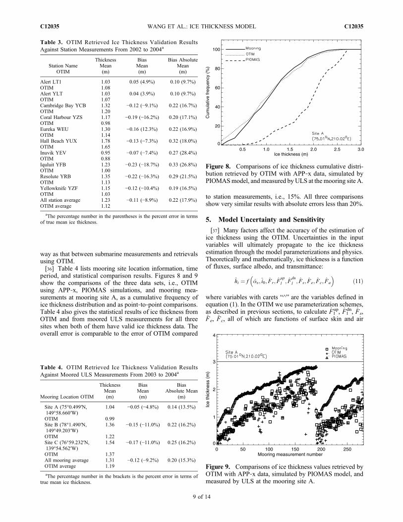
period, and statistical comparison results. Figures 8 and 9show the comparisons of the three data sets, i.e., OTIMusing APP!x, PIOMAS simulations, and mooring mea-surements at mooring site A, as a cumulative frequency ofice thickness distribution and as point!to!point comparisons.Table 4 also gives the statistical results of ice thickness fromOTIM and from moored ULS measurements for all threesites when both of them have valid ice thickness data. Theoverall error is comparable to the error of OTIM compared
to station measurements, i.e., 15%. All three comparisonsshow very similar results with absolute errors less than 20%.
5. Model Uncertainty and Sensitivity
[37] Many factors affect the accuracy of the estimation ofice thickness using the OTIM. Uncertainties in the inputvariables will ultimately propagate to the ice thicknessestimation through the model parameterizations and physics.Theoretically and mathematically, ice thickness is a functionof fluxes, surface albedo, and transmittance:
hi % f !s; i0; Fr; Fupl ; F
dnl ; Fs; Fe; Fc; Fa
' ("11#
where variables with carets “^” are the variables defined inequation (1). In the OTIM we use parameterization schemes,as described in previous sections, to calculate F l
up, F ldn, Fs,
Fe, Fc, all of which are functions of surface skin and air
Table 3. OTIM Retrieved Ice Thickness Validation ResultsAgainst Station Measurements From 2002 to 2004a
aThe percentage number in the parentheses is the percent error in termsof true mean ice thickness.
Table 4. OTIM Retrieved Ice Thickness Validation ResultsAgainst Moored ULS Measurements From 2003 to 2004a
Mooring Location OTIM
ThicknessMean(m)
BiasMean(m)
BiasAbsolute Mean
(m)
Site A (75°0.499"N,149°58.660"W)
1.04 !0.05 (!4.8%) 0.14 (13.5%)
OTIM 0.99Site B (78°1.490"N,149°49.203"W)
1.36 !0.15 (!11.0%) 0.22 (16.2%)
OTIM 1.22Site C (76°59.232"N,139°54.562"W)
1.54 !0.17 (!11.0%) 0.25 (16.2%)
OTIM 1.37All mooring average 1.31 !0.12 (!9.2%) 0.20 (15.3%)OTIM average 1.19
aThe percentage number in the brackets is the percent error in terms oftrue mean ice thickness.
Figure 8. Comparisons of ice thickness cumulative distri-bution retrieved by OTIM with APP!x data, simulated byPIOMASmodel, andmeasured by ULS at the mooring site A.
Figure 9. Comparisons of ice thickness values retrieved byOTIM with APP!x data, simulated by PIOMAS model, andmeasured by ULS at the mooring site A.
WANG ET AL.: ICE THICKNESS MODEL C12035C12035
9 of 14
temperatures (Ts, Ta), surface air pressure (Pa), surface airrelative humidity (R), ice temperature (Ti), wind speed (U),cloud amount (C), and snow depth (hs). Therefore icethickness is actually a function of those variables:
hi % f !s; i0; Fr; T s; T i; T a; Pa; R; U ; C; hs; Fa
' ("12#
[38] The true ice thickness hi is estimated from the truevalues of all the controlling variables in equation (12). Let xirepresent the variables in equation (12) with true values, andlet xi represent those variables with estimated values, withxi subscript i from 1 to 12 representing 12 variables inequation (12). Thus if the uncertainties in the controllingvariables are independent and random, error (hi ! hi) can beexpressed in terms of the uncertainties in the variables onwhich it depends:
hi ! hi' (
%X
xi ! xi" # @hi@xi
; "13#
or the variance in the thickness error, as
"2hi %
X"2xi
@hi@xi
! "2
: "14#
If, however, as discussed by Key et al. [1997b], the variablesare not independent, the covariances between them must beconsidered. Data needed to estimate the covariance betweenall pairs of variables are often not available. If the covariancebetween pairs of variables is unknown, it can be shown[Taylor, 1982] that the total uncertainty follow the rule that
"hi (X
"xi@hi@xi
))))
)))): "15#
[39] Tables 5 and 6 give estimates of the partial deriva-tives needed in equations (13), (14), and (15), computedusing differences (Dhi/Dxi). Mathematically, if we know theexplicit functional relationship between ice thickness and allits arguments, we could derive partial derivative analytically.
However, ice thickness varies nonlinearly with respect to theparameters under investigation, which are parameterizedand/or implicitly involved in the ice thickness calculation, i.e., no explicit functional relationship exists for the analyticalpartial derivation. Therefore we use numerical method tocalculate partial derivatives. These partial derivatives rep-resent the sensitivity of the ice thickness to uncertainties inthe controlling variables. The estimated uncertainties in thecontrolling variables in equation (12), e.g., surface skintemperature Ts, are now used to assess the accuracy of theice thickness estimation using satellite data products. Sinceice thickness varies nonlinearly with respect to the control-ling variables, its sensitivity to uncertainties varies over therange of the input controlling variables. Therefore, accuracyin ice thickness is estimated for a reference ice thickness aslisted in Tables 5 and 6.[40] To estimate shi, we need to first estimate the un-
certainties of all controlling variables in equation (12). Ac-cording to Wang and Key’s [2005] study, for the satelliteretrieved surface broadband albedo as, the uncertaintywould be as large as 0.10 in absolute magnitude. Regardingthe ice slab transmittance i0, we use an absolute uncertaintyof 0.05 in this study, which is probably larger than actualvalue. Satellite retrieved surface downward shortwaveradiation flux Fr can be biased high or low by 20% of theactual value or 35 W m!2 as compared with in situ mea-surements [Wang and Key, 2005]. Wang and Key [2005]also estimated the uncertainties in satellite!derived surface
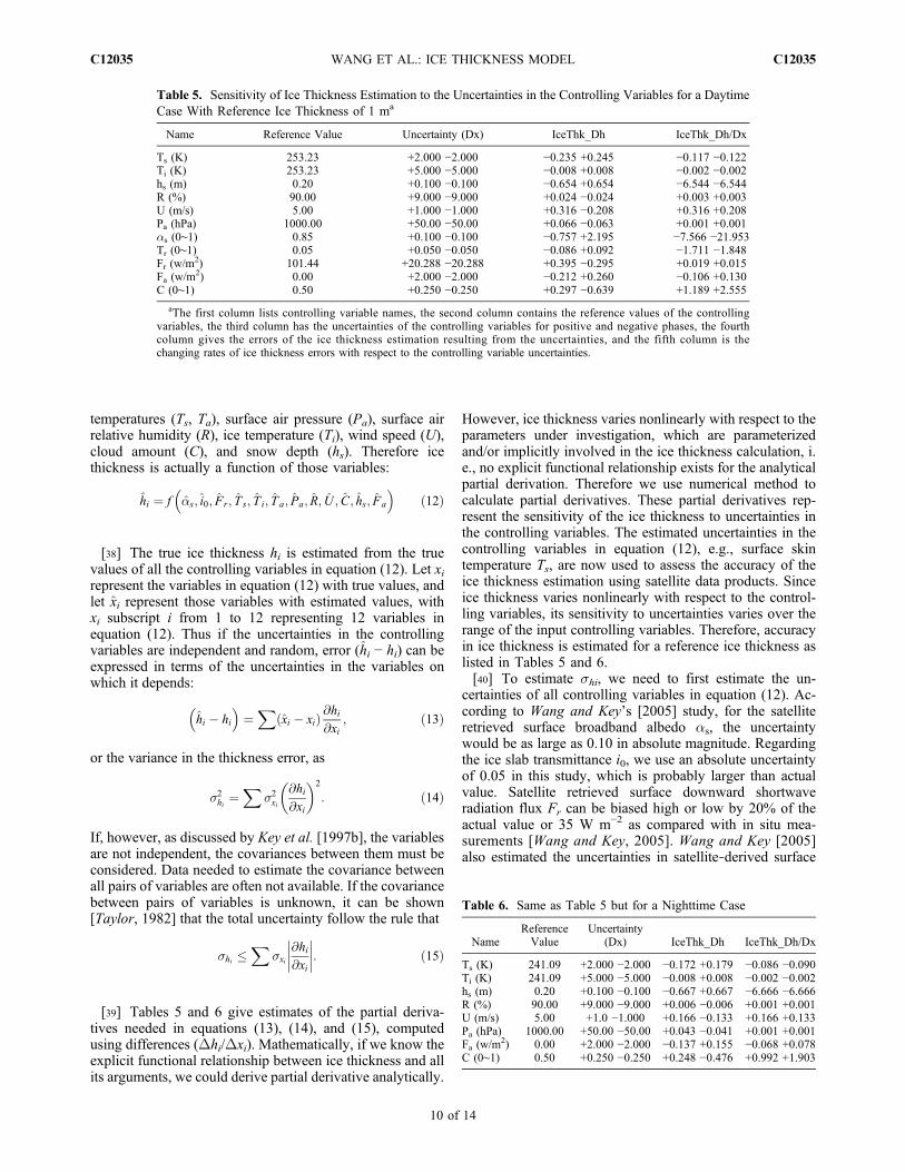
Table 5. Sensitivity of Ice Thickness Estimation to the Uncertainties in the Controlling Variables for a DaytimeCase With Reference Ice Thickness of 1 ma
Name Reference Value Uncertainty (Dx) IceThk_Dh IceThk_Dh/Dx
aThe first column lists controlling variable names, the second column contains the reference values of the controllingvariables, the third column has the uncertainties of the controlling variables for positive and negative phases, the fourthcolumn gives the errors of the ice thickness estimation resulting from the uncertainties, and the fifth column is thechanging rates of ice thickness errors with respect to the controlling variable uncertainties.
skin temperature Ts and cloud amount C with respect to theSurface Heat Balance of the Arctic Ocean (SHEBA) shipmeasurements [Maslanik et al., 2001], and these un-certainties can be as large as 2 K and 0.25 in absolutemagnitude, respectively. We take 2 K as surface air tem-perature Ta uncertainty. Since the surface may be coveredwith a layer of snow, the ice slab temperature Ti may bedifferent from Ts. Assuming Ti equal to Ts may introduceadditional error in ice thickness estimation. We elect toassign 5 K uncertainty in Ti to estimate its impact on the icethickness derivation since there is no information about thedifference between Ti and Ts, and satellite remote sensingcan only retrieve surface skin temperature Ts, not Ti.[41] The uncertainties in surface air pressure and relative
humidity along with surface skin temperature will affect theice thickness estimation indirectly through the impact ofturbulent sensible and latent heat fluxes. A change of 50 hPasurface air pressure may induce changing weather pattern,we take 50 hPa as possible maximum uncertainty of surfaceair pressure. An uncertainty of 10% in surface air relativehumidity is adopted in this work. The uncertainty in geo-strophic wind UG could be 2 m s!1 as determined by thebuoy pressure field [Thorndike and Colony, 1982], and therelationship U = 0.34UG gives the uncertainty in surfacewind speed U of 0.7 m s!1, we take 1 m s!1 as possibleactual uncertainty in this study. Snow on the ice directlyaffects conductive heat flux, surface albedo, and the radia-tive fluxes at the interface of the ice!snow. Snow depth hsplays a very important role, but accurate and spatially widecovered measurements are usually not available coinciden-tally in time and space with satellite observations, and may
change over time with wind and topography. It is difficult toknow the uncertainty in snow depth estimation, and we give50% of the given snow depth as its uncertainty in general.The last uncertainty source is the surface residual heat fluxFa, which is associated with ice melting and possible hori-zontal heat gain/loss. In the case of no melting and nohorizontal heat flux, Fa is zero, which is widely accepted bymany sea ice models if the surface temperature is belowfreezing point. We set uncertainty of Fa 2 W m!2 as aninitial guess. The overall error in the ice thickness estimationcaused by the uncertainties in those controlling variables isless than or equal to the summation of all errors from eachindividual uncertainty source as mathematically describedby equation (15), because the opposite effects may canceleach other.[42] Tables 5 and 6 list the controlling variables, their
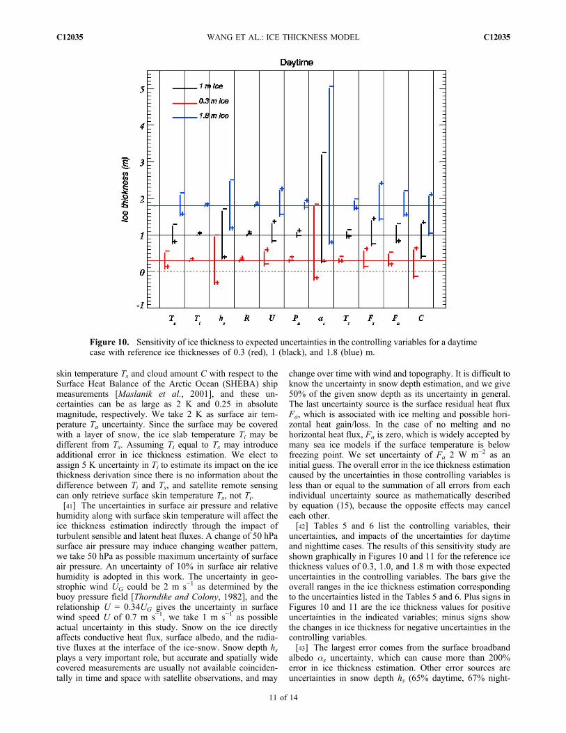
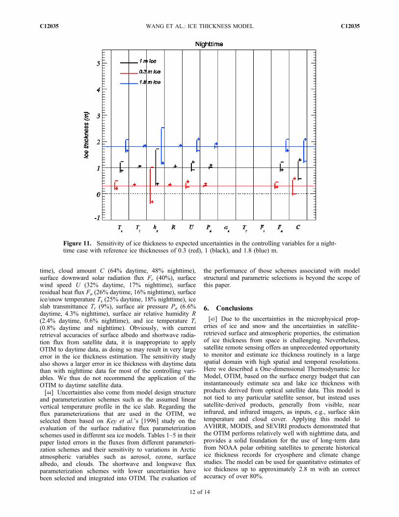
uncertainties, and impacts of the uncertainties for daytimeand nighttime cases. The results of this sensitivity study areshown graphically in Figures 10 and 11 for the reference icethickness values of 0.3, 1.0, and 1.8 m with those expecteduncertainties in the controlling variables. The bars give theoverall ranges in the ice thickness estimation correspondingto the uncertainties listed in the Tables 5 and 6. Plus signs inFigures 10 and 11 are the ice thickness values for positiveuncertainties in the indicated variables; minus signs showthe changes in ice thickness for negative uncertainties in thecontrolling variables.[43] The largest error comes from the surface broadband
albedo as uncertainty, which can cause more than 200%error in ice thickness estimation. Other error sources areuncertainties in snow depth hs (65% daytime, 67% night-
Figure 10. Sensitivity of ice thickness to expected uncertainties in the controlling variables for a daytimecase with reference ice thicknesses of 0.3 (red), 1 (black), and 1.8 (blue) m.
WANG ET AL.: ICE THICKNESS MODEL C12035C12035
11 of 14
time), cloud amount C (64% daytime, 48% nighttime),surface downward solar radiation flux Fr (40%), surfacewind speed U (32% daytime, 17% nighttime), surfaceresidual heat flux Fa (26% daytime, 16% nighttime), surfaceice/snow temperature Ts (25% daytime, 18% nighttime), iceslab transmittance Tr (9%), surface air pressure Pa (6.6%daytime, 4.3% nighttime), surface air relative humidity R(2.4% daytime, 0.6% nighttime), and ice temperature Ti(0.8% daytime and nighttime). Obviously, with currentretrieval accuracies of surface albedo and shortwave radia-tion flux from satellite data, it is inappropriate to applyOTIM to daytime data, as doing so may result in very largeerror in the ice thickness estimation. The sensitivity studyalso shows a larger error in ice thickness with daytime datathan with nighttime data for most of the controlling vari-ables. We thus do not recommend the application of theOTIM to daytime satellite data.[44] Uncertainties also come from model design structure
and parameterization schemes such as the assumed linearvertical temperature profile in the ice slab. Regarding theflux parameterizations that are used in the OTIM, weselected them based on Key et al.’s [1996] study on theevaluation of the surface radiative flux parameterizationschemes used in different sea ice models. Tables 1–5 in theirpaper listed errors in the fluxes from different parameteri-zation schemes and their sensitivity to variations in Arcticatmospheric variables such as aerosol, ozone, surfacealbedo, and clouds. The shortwave and longwave fluxparameterization schemes with lower uncertainties havebeen selected and integrated into OTIM. The evaluation of
the performance of those schemes associated with modelstructural and parametric selections is beyond the scope ofthis paper.
6. Conclusions
[45] Due to the uncertainties in the microphysical prop-erties of ice and snow and the uncertainties in satellite!retrieved surface and atmospheric properties, the estimationof ice thickness from space is challenging. Nevertheless,satellite remote sensing offers an unprecedented opportunityto monitor and estimate ice thickness routinely in a largespatial domain with high spatial and temporal resolutions.Here we described a One!dimensional Thermodynamic IceModel, OTIM, based on the surface energy budget that caninstantaneously estimate sea and lake ice thickness withproducts derived from optical satellite data. This model isnot tied to any particular satellite sensor, but instead usessatellite!derived products, generally from visible, nearinfrared, and infrared imagers, as inputs, e.g., surface skintemperature and cloud cover. Applying this model toAVHRR, MODIS, and SEVIRI products demonstrated thatthe OTIM performs relatively well with nighttime data, andprovides a solid foundation for the use of long!term datafrom NOAA polar orbiting satellites to generate historicalice thickness records for cryosphere and climate changestudies. The model can be used for quantitative estimates ofice thickness up to approximately 2.8 m with an correctaccuracy of over 80%.
Figure 11. Sensitivity of ice thickness to expected uncertainties in the controlling variables for a night-time case with reference ice thicknesses of 0.3 (red), 1 (black), and 1.8 (blue) m.
WANG ET AL.: ICE THICKNESS MODEL C12035C12035
12 of 14
[46] Validation studies indicate that satellite!derivedArctic sea ice thickness using OTIM has a near!zero meanbias (0.02 m) and a mean absolute bias of 0.18 m whencompared to submarine upward looking sonar measure-ments. The overall bias between ice thickness from theOTIM retrievals and in situ station measurements is !0.11 m,with a mean absolute bias of 0.22 m. Mean bias and meanabsolute bias between OTIM retrievals and moored ULSmeasurements are !0.12 m and 0.20 m, respectively. Theestimation error comes from the uncertainties in satellite!derived products, model physics and parameterizations,unknown ice and atmospheric properties, and the inexactcollocation of satellite and in situ measurements. It wasfound that the error tends to be much larger where the icesurface is not smooth, as in the presence of ice ridges,hummocks, or melt ponds. This is not unexpected, as icedynamics are not included in the OTIM. Comparisons withnumerical model simulations demonstrate that the modelsimulated ice thickness is generally overestimated, espe-cially for relatively thin ice.[47] In the presence of solar radiation, it is difficult to
solve the energy budget equation for ice thickness analyti-cally due to the complex interaction of ice/snow physicalproperties with solar radiation, which varies considerablywith changes in ice/snow clarity, density, chemicalscontained, salinity, particle size and shape, and structure.The daytime retrieval is further complicated by inaccuraciesin satellite retrievals of surface albedo and the shortwaveradiation flux, and the Solar heating on the ice plays sig-nificant role in the surface energy budget and makes theresidual heat flux not zero due to partial ice melting andhorizontal heat flux. We are now working on the parame-terization of the surface residual heat flux as a function ofatmospheric and surface conditions, i.e., surface albedo,wind, humidity, surface skin and air temperatures, icethickness, snow depth, cloud amount, and incoming solarradiation flux and/or solar zenith angle, based on stationmeasurements. This way, we will have an OTIM surfaceenergy unbalanced model that will reliably retrieve icethickness with daytime data. At present, we do not recom-mend the application of the current OTIM to daytime data.[48] Applications of the OTIM to satellite data products,
in particular, NOAA polar orbiting satellites, will make itpossible to routinely monitor rapidly changing sea iceconcentration, extent, thickness, and volume, and will pro-vide a better understanding of changes in the cryosphere andclimate.
[49] Acknowledgments. We would like to thank Jinlun Zhang at theUniversity of Washington for providing PIOMAS simulated Arctic sea icethickness data and Zhenglong Li at the University of Wisconsin–Madisonfor helping read out the mooring sea ice draft data in Matlab data format.Thanks also go to the National Snow and Ice Data Center (NSIDC) for pro-viding submarine ice draft data, the Canadian Ice Service (CIS) for provid-ing station!measured Arctic sea ice thickness data, and the Beaufort GyreExploration Program based at the Woods Hole Oceanographic Institution(http://www.whoi.edu/beaufortgyre) for making mooring data availablefor us. Finally, we thank the editors and two anonymous reviewers for theirhelpful comments on the earlier versions of the manuscript. This work waspartially supported by the NOAA GOES!R AWG project and the NPOESSIntegrated Program Office. The views, opinions, and findings contained inthis report are those of the author(s) and should not be construed as an officialNational Oceanic and Atmospheric Administration or U.S. Governmentposition, policy, or decision.
ReferencesAckerman, S. A., K. I. Strabala, W. P.Menzel, R. A. Frey, C. C.Moeller, andL. E. Gumley (1998), Discriminating clear sky from clouds with MODIS,J. Geophys. Res., 103, 32,141–32,157, doi:10.1029/1998JD200032.
Andreas, E. L., and S. F. Ackley (1982), On the differences in ablation sea-sons of Arctic and Antarctic sea ice, J. Atmos. Sci., 39, 440–447,doi:10.1175/1520-0469(1982)039<0440:OTDIAS>2.0.CO;2.
Bennett, T. J. (1982), A coupled atmosphere!sea ice model study of the roleof sea ice in climatic predictability, J. Atmos. Sci., 39, 1456–1465,doi:10.1175/1520-0469(1982)039<1456:ACASIM>2.0.CO;2.
Bentamy, A., K. B. Katsaros, M. Alberto, W. M. Drennan, E. B. Forde, andH. Roquet (2003), Satellite estimates of wind speed and latent heat fluxover the global oceans, J. Clim., 16(4), 637–656, doi:10.1175/1520-0442(2003)016<0637:SEOWSA>2.0.CO;2.
Berliand, T. C. (1960), Method of climatological estimation of global radi-ation, Meteorol. Gidrol., 6, 9–12.
Cavalieri, D., C. Parkinson, P. Gloersen, and H. J. Zwally (2008), Sea iceconcentrations from Nimbus!7 SMMR and DMSP SSM/I passive micro-wave data, digital media, Natl. Snow and Ice Data Cent., Boulder, Colo.
Comiso, J. C. (2002), A rapidly declining perennial sea ice cover in theArctic, Geophys. Res. Lett., 29(20), 1956, doi:10.1029/2002GL015650.
Cox, G. F. N., and W. F. Weeks (1974), Salinity variations in sea ice,J. Glaciol., 13, 109–120.
Curry, A. J., and P. J. Webster (1999), Thermodynamics of Atmospheresand Oceans, 277 pp., Academic, London.
Doronin, Y. P. (1971), Thermal Interaction of the Atmosphere and Hydro-sphere in the Arctic, 85 pp., Isr. Program for Sci. Transl, Jerusalem.
Drobot, S., J. Stroeve, J. Maslanik, W. Emery, C. Fowler, and J. Key (2008),Evolution of the 2007–2008 Arctic sea ice cover and prospects for a newrecord in 2008, Geophys. Res. Lett., 35 , L19501, doi:10.1029/2008GL035316.
Ebert, E., and J. A. Curry (1993), An intermediate one!dimensional ther-modynamic sea ice model for investigating ice!atmosphere interactions,J. Geophys. Res., 98, 10,085–10,109, doi:10.1029/93JC00656.
Efimova, N. A. (1961), On methods of calculating monthly values of netlongwave radiation, Meteorol. Gidrol., 10, 28–33.
Fowler, C., J. Maslanik, T. Haran, T. Scambos, J. Key, and W. Emery(2007), AVHRR Polar Pathfinder twice!daily 5 km EASE!Grid compo-sites V003, digital media, Natl. Snow and Ice Data Cent., Boulder, Colo.
Francis, J. A., and E. Hunter (2007), Drivers of declining sea ice in the Arc-tic winter: A tale of two seas, Geophys. Res. Lett., 34, L17503,doi:10.1029/2007GL030995.
Francis, J. A., W. Chan, D. J. Leathers, J. R. Miller, and D. E. Veron(2009), Winter Northern Hemisphere weather patterns remember summerArctic sea!ice extent, Geophys. Res. Lett., 36, L07503, doi:10.1029/2009GL037274.
Grenfell, T. C. (1979), The effects of ice thickness on the exchange of solarradiation over the polar oceans, J. Glaciol., 22, 305–320.
Grenfell, T. C., and D. K. Perovich (2004), Seasonal and spatial evolutionof albedo in a snow!ice!land!ocean environment, J. Geophys. Res., 109,C01001, doi:10.1029/2003JC001866.
Hall, D. K., J. Key, K. A. Casey, G. A. Riggs, and D. J. Cavalieri (2004),Sea ice surface temperature product from the Moderate Resolution Imag-ing Spectroradiometer (MODIS), IEEE Trans. Geosci. Remote Sens., 42(5), 1076–1087, doi:10.1109/TGRS.2004.825587.
Jacobs, J. D. (1978), Radiation climate of Broughton Island, in EnergyBudget Studies in Relation to Fast!Ice Breakup Processes in Davis Strait,edited by R. G. Barry and J. D. Jacobs, Occas. Pap. 26, pp. 105–120,Inst. of Arctic and Alp. Res., Univ. of Colo., Boulder.
Jin, Z., K. Stamnes, and W. F. Weeks (1994), The effect of sea ice on thesolar energy budget in the atmosphere!sea ice!ocean system: A modelStudy, J. Geophys. Res., 99(C12), 25,281–25,294, doi:10.1029/94JC02426.
Kara, A. B., P. A. Rochford, and H. E. Hurlburt (2000), Efficient and accu-rate bulk parameterizations of air!sea fluxes for use in general circulationmodels, J. Atmos. Oceanic Technol., 17, 1421–1438.
Kemp, J., K. Newhall, W. Ostrom, R. Krishfield, and A. Proshutinsky(2005), The Beaufort Gyre Observing System 2004: Mooring recoveryand deployment operations in pack ice, Tech. Rep. Woods Hole Ocea-nogr. Inst. WHOI!2005!05, 33 pp., Woods Hole, Mass., doi:10.1575/1912/73.
Key, J. (2002), The Cloud and Surface Parameter Retrieval (CASPR), 62pp., System for Polar AVHRR Data User’s Guide, Space Science andEngineering Center, Univ. of Wisc., Madison.
Key, J. R., R. A. Silcox, and R. S. Stone (1996), Evaluation of surfaceradiative flux parameterizations for use in sea ice models, J. Geophys.Res., 101(C2), 3839–3849, doi:10.1029/95JC03600.
WANG ET AL.: ICE THICKNESS MODEL C12035C12035
13 of 14
Key, J., J. Collins, C. Fowler, and R. Stone (1997a), High!latitude surfacetemperature estimates from thermal satellite data, Remote Sens. Environ.,61, 302–309, doi:10.1016/S0034-4257(97)89497-7.
Key, J., A. J. Schweiger, and R. S. Stone (1997b), Expected uncertainty insatellite!derived estimates of the surface radiation budget at high lati-tudes, J. Geophys. Res., 102(C7), 15,837–15,847, doi:10.1029/97JC00478.
Kovacs, A. (1996), Sea ice: Part I. Bulk salinity versus ice floe thickness,CRREL Rep. 96!7, U.S. Army Cold Reg. Res. and Eng. Lab., Hanover,N. H.
Kwok, R., and G. F. Cunningham (2008), ICESat over Arctic sea ice: Esti-mation of snow depth and ice thickness, J. Geophys. Res., 113, C08010,doi:10.1029/2008JC004753.
Kwok, R., G. F. Cunningham, M. Wensnahan, I. Rigor, H. J. Zwally, andD. Yi (2009), Thinning and volume loss of the Arctic Ocean sea icecover: 2003–2008, J. Geophys. Res., 114, C07005, doi:10.1029/2009JC005312.
Laevastu, T. (1960), Factors affecting the temperature of the surface layerof the sea, Comments Phys. Math., 25(1), 136 pp.
Laxon, S., N. Peacock, and D. Smith (2003), High interannual variability ofsea ice thickness in the Arctic region, Nature , 425, 947–950,doi:10.1038/nature02050.
Lindsay, R. W. (1998), Temporal variability of the energy balance of thickArctic pack ice, J. Clim., 11, 313–333, doi:10.1175/1520-0442(1998)011<0313:TVOTEB>2.0.CO;2.
Liu, Y. H., J. R. Key, R. A. Frey, S. A. Ackerman, and W. P. Menzel(2004), Nighttime polar cloud detection with MODIS, Remote Sens.Environ., 92, 181–194, doi:10.1016/j.rse.2004.06.004.
Maslanik, J. A., J. Key, C. W. Fowler, T. Nguyen, and X. Wang (2001),Spatial and temporal variability of satellite!derived cloud and surfacecharacteristics during FIRE!ACE, J. Geophys. Res., 106(D14),15,233–15,249, doi:10.1029/2000JD900284.
Maslanik, J. A., C. Fowler, J. Stroeve, S. Drobot, J. Zwally, D. Yi, andW. Emery (2007), A younger, thinner Arctic ice cover: Increasedpotential for rapid extensive sea!ice loss, Geophys. Res. Lett., 34,L24501, doi:10.1029/2007GL032043.
Maykut, G. A., and P. E. Church (1973), Radiation climate of Barrow,Alaska, 1962–66, J. Appl. Meteorol., 12, 620–628, doi:10.1175/1520-0450(1973)012<0620:RCOBA>2.0.CO;2.
Maykut, G. A., and N. Untersteiner (1971), Some results from a time!dependent thermodynamic model of sea ice, J. Geophys. Res., 76,1550–1575, doi:10.1029/JC076i006p01550.
Moritz, R. E. (1978), A model for estimating global solar radiation, inEnergy Budget Studies in Relation to Fast!Ice Breakup Processes in Da-vis Strait, edited by R. G. Barry and J. D. Jacobs, Occas. Pap. 26, pp.121–142, Inst. of Arctic and Alp. Res., Univ. of Colo., Boulder.
National Snow and Ice Data Center (2006), Submarine upward lookingsonar ice draft profile data and statistics, digital media, World Data Cent.for Glaciol., Boulder, Colo.
Ohmura, A. (1981), Climate and energy balance of the Arctic tundra,Zürcher Geogr. Schr. 3, 448 pp., Geogr. Inst., Zurich, Switzerland.
Ostrom, W., J. Kemp, R. Krishfield, and A. Proshutinsky (2004), BeaufortGyre Freshwater Experiment: Deployment Operations and Technology in2003, Tech. Rep. Woods Hole Oceanogr. Inst. WHOI!2004!01, 32 pp.,Woods Hole, Mass.
Persson, P. O. G., C. W. Fairall, E. L. Andreas, P. S. Guest, and D. K.Perovich (2002), Measurements near the Atmospheric Surface FluxGroup tower at SHEBA: Near!surface conditions and surface energybudget, J. Geophys. Res., 107(C10), 8045, doi:10.1029/2000JC000705.
Rees, W. G. (1993), Infrared emissivities of Arctic land cover types, Int. J.Remote Sens., 14, 1013–1017, doi:10.1080/01431169308904392.
Rothrock, D., D. B. Percival, and M. Wensnahan (2008), The decline inarctic sea!ice thickness: Separating the spatial, annual, and interannualvariability in a quarter century of submarine data, J. Geophys. Res.,113, C05003, doi:10.1029/2007JC004252.
Saloranta, T. M. (2000), Modeling the evolution of snow, snow ice and icein the Baltic Sea, Tellus, Ser. A, 52, 93–108.
Schmetz, P. J., and E. Raschke (1986), Estimation of daytime downwardlongwave radiation at the surface from satellite and grid point data, Theor.Appl. Climatol., 37, 136–149, doi:10.1007/BF00867847.
Shine, K. P. (1984), Parameterization of shortwave flux over high albedosurfaces as a function of cloud thickness and surface albedo, Q. J. R. Me-teorol. Soc., 110, 747–764, doi:10.1002/qj.49711046511.
Shine, K. P., and A. Henderson!Sellers (1985), The sensitivity of a thermo-dynamic sea ice model to changes in surface albedo parameterization,J. Geophys. Res., 90, 2243–2250, doi:10.1029/JD090iD01p02243.
Taylor, J. R. (1982), An Introduction to Error Analysis, 270 pp., Univ. Sci.Books, Mill Valley, Calif.
Thorndike, A. S., and R. Colony (1982), Sea ice motion in response to geo-strophic winds, J. Geophys. Res., 87(C8), 5845–5852, doi:10.1029/JC087iC08p05845.
Untersteiner, N. (1964), Calculations of temperature regime and heat budgetof sea ice in the central Arctic, J. Geophys. Res., 69, 4755–4766,doi:10.1029/JZ069i022p04755.
Wang, X., and J. Key (2003), Recent trends in Arctic surface, cloud, andradiation properties from space, Science, 299(5613), 1725–1728,doi:10.1126/science.1078065.
Wang, X., and J. Key (2005), Arctic surface, cloud, and radiation propertiesbased on the AVHRR Polar Pathfinder data set. Part I: Spatial and tem-poral characteristics, J. Clim., 18(14), 2558–2574, doi:10.1175/JCLI3438.1.
Wang, X., J. R. Key, C. Fowler, and J. Maslanik (2007), Diurnal cycles inArctic surface radiative fluxes in a blended satellite!climate reanalysis dataset: Algorithm description, validations, and preliminary results, J. Appl.Remote Sens., 1, 013535, doi:10.1117/1.2794003.
Yen, Y.!C. (1981), Review of thermal properties of snow, ice and sea ice,CRREL Rep. 81!10, 27 pp., Cold Reg. Res. and Eng. Lab., Hanover, N. H.
Yu, Y., and D. A. Rothrock (1996), Thin ice thickness from satellite ther-mal imagery, J. Geophys. Res., 101(C11), 25,753–25,766, doi:10.1029/96JC02242.
Zhang, J., and D. A. Rothrock (2001), A thickness and enthalpy distribu-tion sea!ice model, J. Phys. Oceanogr., 31, 2986–3001, doi:10.1175/1520-0485(2001)031<2986:ATAEDS>2.0.CO;2.
Zhang, J., and D. A. Rothrock (2003), Modeling global sea ice with a thick-ness and enthalpy distribution model in generalized curvilinear coordi-nates, Mon. Weather Rev., 131(5), 845–861, doi:10.1175/1520-0493(2003)131<0845:MGSIWA>2.0.CO;2.
Zhang, X., and J. E. Walsh (2006), Toward seasonally ice!covered ArcticOcean: Scenarios from the IPCC AR4 model simulations, J. Clim., 19,1730–1747, doi:10.1175/JCLI3767.1.
Zillman, J. W. (1972), A study of some aspects of the radiation and heatbudgets of the southern hemisphere oceans, Meteorol. Stud. Rep. 26,Bur. of Meteorol., Dep. of the Inter., Canberra.
Zwally, H. J., D. Yi, R. Kwok, and Y. Zhao (2008), ICESat measurementsof sea ice freeboard and estimates of sea ice thickness in the Weddell Sea,J. Geophys. Res., 113, C02S15, doi:10.1029/2007JC004284.
J. R. Key, NESDIS, NOAA, 1225 W. Dayton St., Madison, WI 53706,USA.Y. Liu and X. Wang, Cooperative Institute of Meteorological Satellite
Studies, University of Wisconsin–Madison, 1225 W. Dayton St.,Madison, WI 53706, USA. ([email protected])