Page 1
A Three-State Recursive Sequential Bayesian Algorithm
for Biosurveillance
K. D. Zamba a Panagiotis Tsiamyrtzis b Douglas M. Hawkins c
a Department of Biostatistics, The University of Iowa, 200 Hawkins Drive, C22M GH
Iowa City, IA 52242b Department of Statistics, Athens University of Economics and Business; 76 Patission Str 10434 Athens
Greecec School of Statistics, University of Minnesota, 313 Ford Hall, 224 Church Street Minneapolis, MN 55455
Abstract
A serial signal detection algorithm is developed to monitor pre-diagnosis and medical
diagnosis data pertaining to biosurveillance. The algorithm is three-state sequential,
based on Bayesian thinking. It accounts for non-stationarity, irregularity, seasonality,
and captures an epidemic serial structural details. At stage n, a trichotomous variable
governing the states of an epidemic is defined, and a prior distribution for time-indexed
serial readings is set. The technicality consists of finding a posterior state probability
based on the observed data history, using the posterior as a prior distribution for stage
n + 1 and sequentially monitoring surges in posterior state probabilities. A sensitivity
analysis for validation is conducted and analytical formulas for the predictive distribu-
tion are supplied for error management purposes. The method is applied to syndromic
surveillance data gathered in the United States (U.S.) District of Columbia metropoli-
tan area.
Keywords: Bayesian Sequential Update, Dynamic Control, Syndromic Surveillance.
1 Introduction
The problem that led to developing the method herein came from medical arena. Data
pertaining to biosurveillance are used in the U.S. and in some countries around the globe to
1
Page 2
assess data-driven evidence for natural epidemics or intentional release of biological agents
with operations similar to natural epidemics. With the view of responding to the serious
danger of bioterrorism, there has been a shift in disease surveillance from the classical ret-
rospective disease chart review, to a prospective and real-time early disease detection. In
syndromic surveillance for example, investigators monitor non-specific clinical information
that may indicate bioterrorism associated disease before specific diagnoses are made. Med-
ical related data such as emergency room observations, over-the-counter sales, veterinary
data, medical and public health information, are used as investigational tools to screen out
information about outbreaks and augment early reports to sentinels. Relevant publications
describing the need to integrate medical related data into real-time surveillance systems are
Arnon et al. (2001); Dennis et al. (2001); Henderson et al. (1999); Inglesby et al. (1999,
2000). An overview of the use of syndromic surveillance can be found in Buehler et al.
(2003); overviews and examples of syndromic surveillance systems are found in Green and
Kaufman (2002); and description of the steps of disease outbreak investigation and syndromic
surveillance are described in Pavlin (2003).
Statistical process control (SPC) tools have long time been central parts of classical
disease surveillance and laboratory based outbreak detections. It is to be noted that the U.S.
Center for Disease Control (CDC) has routinely applied cumulative sum (Cusum) techniques
to laboratory-based data for outbreak detection; see for example Hutwagner et al. (1997),
Stern and Lightfoot (1999). These tools though, need extra maintenance if they were to
migrate to the field of modern biosurveillance. Biosurveillance data are not like industrial
and laboratory data for which traditional SPC methods are developed; they fail to meet
most underlying assumptions of SPC. For example, the main parameters associated with
incidence in syndromic surveillance may be unknown, or only partially known, or unstable
and may change a course from year to year. In addition, incidence parameters may jump at
any time and in any direction (upward/downward or stable). It has been recognized that
for some infectious diseases with seasonal trend such as influenza, each season is likely to
generate its specific data pattern; a new data process to be studied de novo.
A critical requirement for biosurveillance algorithms is fast detection. This requirement
is quickly clouded by a background of variability and structural changes depicted on bio-
surveillance data. As common feature, these data substantially violate the various statistical
underpinnings of standard SPC techniques (we refer a reader less familiar with SPC methods
in medical surveillance to Woodall, 2006; Zamba et al., 2008; Shmueli and Burkom, 2010 for
works and in-depth discussions on assumptions and their violations). To explain, as back-
2
Page 3
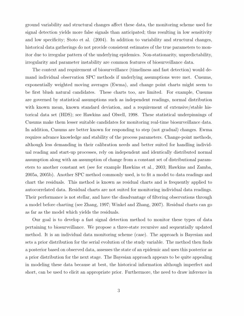
ground variability and structural changes affect these data, the monitoring scheme used for
signal detection yields more false signals than anticipated; thus resulting in low sensitivity
and low specificity; Stoto et al. (2004). In addition to variability and structural changes,
historical data gatherings do not provide consistent estimates of the true parameters to mon-
itor due to irregular pattern of the underlying epidemics. Non-stationarity, unpredictability,
irregularity and parameter instability are common features of biosurveillance data.
The context and requirement of biosurveillance (timeliness and fast detection) would de-
mand individual observation SPC methods if underlying assumptions were met. Cusums,
exponentially weighted moving averages (Ewma), and change point charts might seem to
be first blush natural candidates. These charts too, are limited. For example, Cusums
are governed by statistical assumptions such as independent readings, normal distribution
with known mean, known standard deviation, and a requirement of extensive/stable his-
torical data set (HDS); see Hawkins and Olwell, 1998. These statistical underpinnings of
Cusums make them lesser suitable candidates for monitoring real-time biosurveillance data.
In addition, Cusums are better known for responding to step (not gradual) changes. Ewma
requires advance knowledge and stability of the process parameters. Change-point methods,
although less demanding in their calibration needs and better suited for handling individ-
ual reading and start-up processes, rely on independent and identically distributed normal
assumption along with an assumption of change from a constant set of distributional param-
eters to another constant set (see for example Hawkins et al., 2003; Hawkins and Zamba,
2005a, 2005b). Another SPC method commonly used, is to fit a model to data readings and
chart the residuals. This method is known as residual charts and is frequently applied to
autocorrelated data. Residual charts are not suited for monitoring individual data readings.
Their performance is not stellar, and have the disadvantage of filtering observations through
a model before charting (see Zhang, 1997; Winkel and Zhang, 2007). Residual charts can go
as far as the model which yields the residuals.
Our goal is to develop a fast signal detection method to monitor these types of data
pertaining to biosurveillance. We propose a three-state recursive and sequentially updated
method. It is an individual data monitoring scheme (case). The approach is Bayesian and
sets a prior distribution for the serial evolution of the study variable. The method then finds
a posterior based on observed data, assesses the state of an epidemic and uses this posterior as
a prior distribution for the next stage. The Bayesian approach appears to be quite appealing
in modeling these data because at best, the historical information although imperfect and
short, can be used to elicit an appropriate prior. Furthermore, the need to draw inference in
3
Page 4
an online fashion even in a presence of a short run, along with the possibility of deriving the
predictive distribution for the future observable(s) make the Bayesian approach a favorable
alternative to traditional SPC methods.
The manuscript is organized as follow: Section 2 defines our proposed three-state model
and the algebraic formulas governing the states at each stage. Section 3 elaborates on the
attractiveness of our model, its novelty and its reproducibility. Section 4 outlines our simu-
lation results, the sensitivity analysis, and applies our approach to real-time data gathered
in the U.S. We close our paper with sections on comparative study, discussion and technical
appendix.
2 Proposed Three-State Bayesian Statistical Modeling
We assume that observations are gathered sequentially and define a time indexed series
Yn, n = 1, 2, . . .; where n may be hours, days, weeks, months, . . . , depending on the impor-
tance of the characteristic being monitored. The observed Yn may be actual case counts or
percentage of some activity observed, standardized observed cases, or any aggregation of ob-
served data over a specific hospital, location county, or state. We work under the assumption
that readings are large enough for normality to hold.
At time n = 0, before any monitoring starts, we set a prior distribution for the response
variable; we denote this by Y0:
Y0 ∼ N(ζ, σ20),
where ζ and σ20 are the initial prior mean and variance, assumed known. The prior infor-
mation, although imperfect, may come from an educated guess, from previous HDS or from
expert’s opinion.
Moving between successive stages n−1 and n, we model Yn using a first order autoregressive
AR(1) model:
Yn = λYn−1 + un, (1)
where λ ∈ (0, 1) is a discount factor, assumed to be known, and un is a random error
displacement. Observe that for λ = 0, the model becomes the random batch effect model
while for λ = 1 the model is a random walk model. The AR representation provides a smooth
transition between successive stages, relaxing the independence assumption governing most
standard SPC techniques. The three-state approach comes as follow: Yn may be affected by
three mutually exclusive states; flat, rise and decay.
• Flat state: Yn does not change much from Yn−1
4
Page 5
• Rise state: Yn experiences positive jumps/shocks with respect to Yn−1
• Decay state: Yn experiences negative jumps/shocks with respect to Yn−1.
We model these three states using a trichotomous random variable En. Specifically, at each
stage n one has:
En =
0 with prob. π(n−1)0
−1 with prob. π(n−1)−
+1 with prob. π(n−1)+
, (2)
with 0,−1 and +1 indicating flat, decay and rise states respectively; each of which occurs
with some a-priori probability(π
(n−1)0 + π
(n−1)− + π
(n−1)+ = 1
).
Each realization of En corresponds to either a jump (for the En = ±1) or a no-jump
(En = 0) scenario. For the cases where a jump occurs (i.e. rise or decay states) we consider
the size of the jump to be a random variable with directionality given by the sign of En (the
direction is upward for the rise and downward for the decay states). If δn denotes the size of
the jump at time n, we assume:
δn ∼ N(∆, τ 2),
where ∆ is the expected magnitude of the jump, and τ 2 is the uncertainty regarding the prior
mean estimate ∆. In this setting we have selected the same expected magnitude for both the
rise and the decay because of the hallmark of our illustrative epidemics under study. One
may choose different magnitudes, ∆1 for rise and ∆2 for decay, based on a specific epidemic
or upon observing the shape of an epidemic curve using a small but relevant HDS.
Brief, En is a trichotomous random variable associated with the directionality of Yn and
governs the states, while δn is associated with the size of the random shock. Both these
entities are embedded in the random error displacement un of Equation (1) as follows:
un|(En, δn) ∼ N(Enδn, σ2);
yielding an unconditional distribution of random error un of
un ∼
N( 0, σ2) with prob. π(n−1)0
N(−∆, σ2 + τ 2) with prob. π(n−1)−
N(+∆, σ2 + τ 2) with prob. π(n−1)+
.
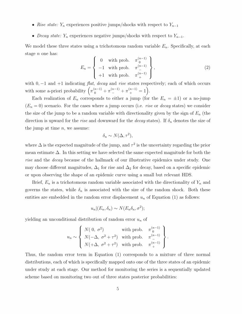
Thus, the random error term in Equation (1) corresponds to a mixture of three normal
distributions, each of which is specifically mapped onto one of the three states of an epidemic
under study at each stage. Our method for monitoring the series is a sequentially updated
scheme based on monitoring two out of three states posterior probabilities:
5
Page 6
• At stage n, get the observation Yn and obtain the posterior En|Yn .
• Draw a decision regarding the state of the epidemics, based on the posterior distribution
and obtain the predictive distribution.
• Continue monitoring if the posterior distribution is within the ‘range of acceptability’
(point to which we will return).
• Use the posterior distribution at stage n as a prior distribution for stage n+1 (sequential
update).
In Equation (2), the probabilities π(n−1)0 , π
(n−1)− and π
(n−1)+ require some attention. These
respectively refer to the posterior probabilities of flat, decay and rise states of an epidemic
at time point n − 1. For this scheme to be able to run, one needs to set some initial
prior probabilities π(0)0 , π
(0)− and π
(0)+ which reflect prior beliefs regarding the states of an
epidemic at time 0. In the event that no such prior belief exists, one can simply choose a
non-informative prior such as π(0)0 = π
(0)− = π
(0)+ = 1/3.
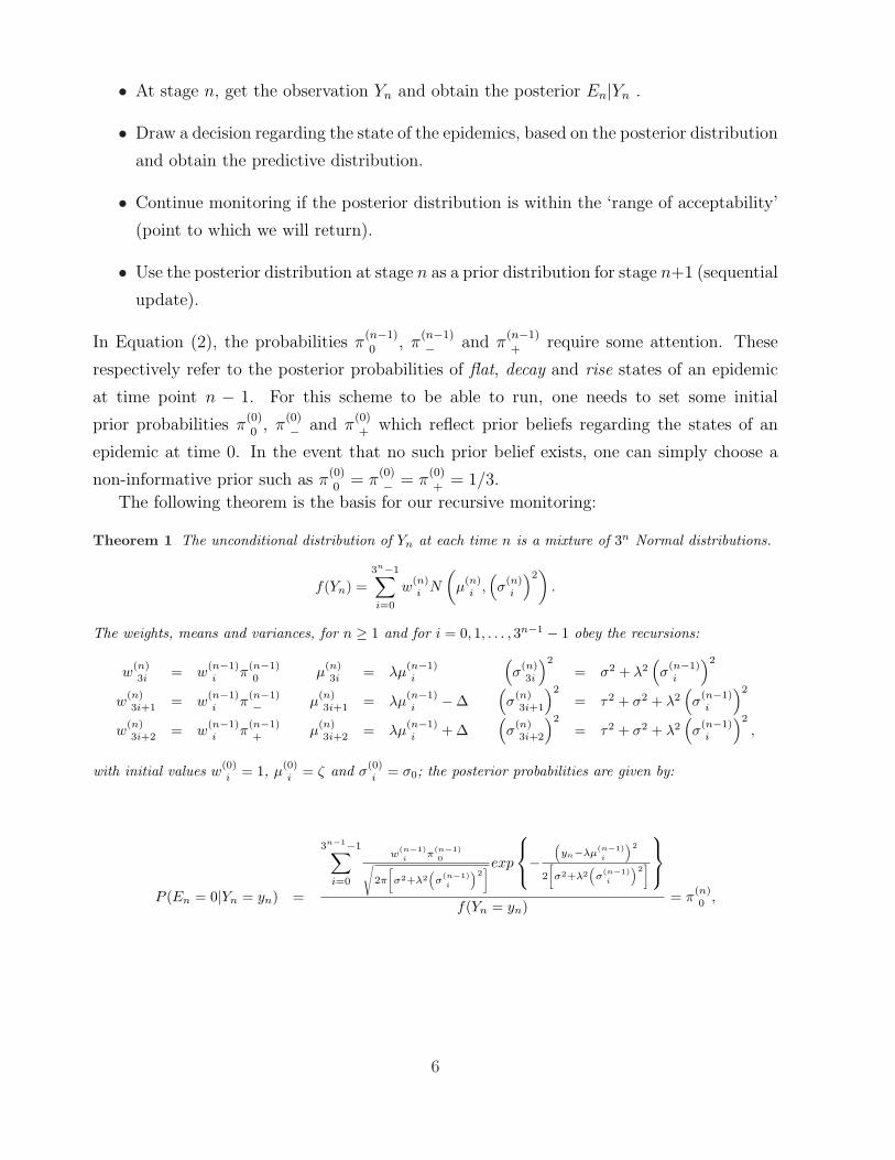
The following theorem is the basis for our recursive monitoring:
Theorem 1 The unconditional distribution of Yn at each time n is a mixture of 3n Normal distributions.
f(Yn) =3n−1∑
i=0
w(n)i N
(µ
(n)i ,
(σ
(n)i
)2)
.
The weights, means and variances, for n ≥ 1 and for i = 0, 1, . . . , 3n−1 − 1 obey the recursions:
w(n)3i = w
(n−1)i π
(n−1)0 µ
(n)3i = λµ
(n−1)i
(σ
(n)3i
)2
= σ2 + λ2(σ
(n−1)i
)2
w(n)3i+1 = w
(n−1)i π
(n−1)− µ
(n)3i+1 = λµ
(n−1)i −∆
(σ
(n)3i+1
)2
= τ2 + σ2 + λ2(σ
(n−1)i
)2
w(n)3i+2 = w
(n−1)i π
(n−1)+ µ
(n)3i+2 = λµ
(n−1)i + ∆
(σ
(n)3i+2
)2
= τ2 + σ2 + λ2(σ
(n−1)i
)2
,
with initial values w(0)i = 1, µ
(0)i = ζ and σ
(0)i = σ0; the posterior probabilities are given by:
P (En = 0|Yn = yn) =
3n−1−1∑
i=0
w(n−1)i
π(n−1)0√
2π
[σ2+λ2
(σ
(n−1)i
)2]exp
−
(yn−λµ
(n−1)i
)2
2
[σ2+λ2
(σ
(n−1)i
)2]
f(Yn = yn)= π
(n)0 ,
6
Page 7
P (En = −1|Yn = yn) =
3n−1−1∑
i=0
w(n−1)i
π(n−1)−√
2π
[τ2+σ2+λ2
(σ
(n−1)i
)2]exp
−
(yn−
[λµ
(n−1)i
−∆])2
2
[τ2+σ2+λ2
(σ
(n−1)i
)2]
f(Yn = yn)= π
(n)− , and
P (En = +1|Yn = yn) =
3n−1−1∑
i=0
w(n−1)i
π(n−1)+√
2π
[τ2+σ2+λ2
(σ
(n−1)i
)2]exp
−
(yn−
[λµ
(n−1)i
+∆])2
2
[τ2+σ2+λ2
(σ
(n−1)i
)2]
f(Yn = yn)= π
(n)+ .
For proof of the theorem, see technical appendix -A.
Note that the formulas in this theorem are all recursive. In particular, P (En | Yn = yn) is
derived with the use of the prior at stage n−1 (that involves information about yn−1) which
is, on itself, an updated posterior coming from stage n− 2 and so on. Therefore, historical
data information is maintained and updated as each new observation yn accrues. Other
points that remain to be exposed from the theorem are the subscripts and the superscripts
of the iterative weights, means and variances. The subscript i denotes each component of
the mixture at stage n − 1; i ∈ {0, 1, . . . , 3n−1 − 1}. As one moves from n − 1 to n, each
i triplicates, giving rise to a mixture of 3 × 3n−1 = 3n components. To keep track of the
flat− rise− decay cases and facilitate their recognition, the components are renumbered at
time n using the module 3 operator, i.e.:
3i + 0 refers to the flat state (corresponding to mod(3)=0)
3i + 1 refers to the decay state (corresponding to mod(3)=1)
3i + 2 refers to the rise state (corresponding to mod(3)=2).
Thus, the modulo 3 operator allows us to easily discriminate which of the components refers
to what of the three possible states of the epidemic. The problem of monitoring the time-
indexed series comes down to estimating and monitoring two of the three π(n)• ’s.
2.1 Drawing Decision Regarding the State of the Epidemic
In General: At each stage of the sequential algorithm, three actions may be taken. The
actions a(n)f , a
(n)r and a
(n)d are respectively associated with the flat, rise, and decay states
of the epidemic at stage n. Some of these actions may be: reinforcing current measures of
preparedness, taking stronger eradicative measures, or allocating resources to other means.
Depending on whether π(n)• (i.e. any state posterior probability at stage n) has actually
increased, decreased, or stabilized, there would be some costs incurred. A loss matrix such
7
Page 8
as in Table 1 can be built and decision rules for hypotheses testing can be worked into the
sequential algorithm. Note that a Bayes rule always exists since the action space is a compact
set.
a(n)d a
(n)f a
(n)r
En = −1 0 c−1,f c−1,r
En = 0 c0,d 0 c0,r
En = +1 c1,d c1,f 0
Table 1: Loss matrix for a more general decision problem. In the matrix, c•,• represents the costs associated
with the true state of En (denoted by the first subscript) and the action taken (second subscript).
Expert’s opinion may be used to provide the appropriate values for the loss matrix. Once
the matrix is set, one can derive the ‘optimal’ decision, according to some criterion, like Bayes
risk, Minimax rule or other similar optimality criteria (see for example De Groot, 1970 and
Berger, 1980).
Special case: In the following special case, we are interested in detecting the rise state of
the epidemic (which in public health is usually of highest importance) while controlling the
false alarm rate. This corresponds to the sequential hypothesis testing:
{H
(n)0 : En = +1
H(n)1 : En 6= +1
}.
Denote a(n)0 and a
(n)1 the decisions to accept H
(n)0 and H
(n)1 respectively. Also, denote cMA
the cost associated with the ‘Missed Alarm’ (failing to recognize the rise, or Type I error);
and cFA the one associated with ‘False Alarm’ (falsely claiming a rise, or Type II error).
The loss matrix becomes a 2 × 2 matrix, and according to the generalized 0–1 loss function
takes the form of Table 2.
a(n)0 a
(n)1
En = +1 0 cMA
En 6= +1 cFA 0
Table 2: Loss matrix generated by the 0–1 generalized loss function principle for the special decision
problem.
8
Page 9
It is then easy to show (Casela and Berger, 1990) that the Bayes decision rule (i.e. the
decision which minimizes Bayes risk) is: ‘Reject H(n)0 if and only if’
P (En = +1|Yn) <cFA
cMA + cFA
.
We should note here that other decision drawing methods such as Bayes factors (Jeffreys,
1948) are also plausible.
2.2 Thresholding the Posterior Probabilities
As noted earlier, the method is a sequentially updated recursive scheme where at stage n,
the posterior probability of each state is used as prior for stage n+1. This technique invites
a natural problem where one state with a history of consecutively low probabilities con-
stantly contaminates its subsequent updates. This problem is known as causing sensitivity
issues because a very low prior probability of an unlikely state would need several succes-
sive observations with high likelihood to provide an accurate signal. To avoid this problem,
one usually puts a ‘floor’ on the value of a prior probability of any state; a technique that
provides ‘head start’ to speed response to signal. The idea consists of defining a threshold
floor value p∗ such that π(n)• = max
{p∗, π(n)
•
}, and adjusting the remaining probabilities to
attain collective exhaustiveness.
3 Attractiveness and Novelty of the Method
The attractiveness of the Bayesian method lies in its ease of adaptability to parameter in-
stability such as the one seen in syndromic surveillance data settings. Bayesian approaches
appear to be quite appealing in modeling these data because at least, the historical informa-
tion (although usually imperfect) can be used to elicit an appropriate prior. Furthermore, in
disease surveillance there is a need to draw inference in an online fashion even in a presence
of a short data history. Our algorithm has the flexibility of a straightforward transition from
fixed to a random jump. The sequential updating mechanism has allowed our approach
to also perform well in the presence of a non informative prior for the state probabilities.
Another appealing aspect is the possibility of deriving predictive distribution for future ob-
servable(s) to be used for error management or forecasting purposes. Specifically, following
Geisser (1993) we easily show via some algebra (see technical appendix) that the predictive
distribution of Yn given the available data Y1, . . . , Yn−1 is a mixture of 3n Normal components:
9
Page 10
f(Yn|Yn−1) ∼∑
i∈{0,−1,+1}f(Yn|En = i)P (En = i|Yn−1)
∼3n−1−1∑
i=0
[w
(n−1)i π
(n−1)0 N
(λµ
(n−1)i , σ2 + λ2
(σ
(n−1)i
)2)
+ w(n−1)i π
(n−1)− N
(λµ
(n−1)i −∆, τ 2 + σ2 + λ2
(σ
(n−1)i
)2)
+ w(n−1)i π
(n−1)+ N
(λµ
(n−1)i + ∆, τ 2 + σ2 + λ2
(σ
(n−1)i
)2)]
.
This distribution opens the door to the predictive advantage of our mechanism.
We view our proposal as a self-reliant algorithm in that it combines three different aspects
of control theory into a single process. It has the flexibility to simultaneously model, chart,
and forecast. Modeling comes about by deriving the unconditional mixture distribution Yn,
sequential charting intervenes by taking advantage of the posterior state probabilities, and
forecasting becomes apparent by making an adequate usage of the predictive distribution of
Yn.
3.1 Computational Considerations and Reproducibility
In an era of advanced computational technology, one may be tempted to implement our
methodology in a ‘brute-force’ manner. However, direct implementation of the mixtures
involved in the theorem, and their sequential computation can lead to much severe compu-
tational load than necessary. The use of the three-state approach to modeling En induces
a mixture of 3n Normal components in the unconditional distribution of Yn. Thus, we have
a combinatorial explosion of the number of components used to describe the process. The
reason for this explosion is that the model attempts to keep all possible trajectories from the
beginning of the process till the most recent observation. Due to the autoregressive nature of
the model, the posterior mixture parameters are bounded (see technical appendix A for these
bounds). As n increases, the 3n components have tiny weights and their parameters differ
only slightly. Thus, we approximate the exact distribution with another mixture having
far fewer components. We adopt the approximation algorithm of Tsiamyrtzis and Hawkins
(2010), which is a hybrid of the procedure proposed in West (1993).
First select K, as the number of components for the approximating mixture. At stage n of
the process, when the number of components r = 3n exceeds K for first time, activate the
10
Page 11
approximation algorithm:
1. Sort the r components in increasing order of their weights.
2. Find the index i (i = 2, 3, . . . , r) of the ‘nearest neighbor’ of component 1.
3. Replace these two distributions with a new Normal with updated parameters. Set
r = r − 1.
4. Go to step 1 and repeat the procedure, until r = K.
Two issues that need to be clarified here are the definition of a ‘nearest neighbor’ (step 2)
and the replacement of two Normal components by a single one (step 3).
To measure distribution proximity in finding the nearest neighbor (required at stage 2
of the algorithm), we use the Jeffreys (1948) divergence measure. Specifically, the Jeffreys
divergence between f1 and f2 is provided by:
J(f1, f2) =
∫[f1(x)− f2(x)] log
(f1(x)
f2(x)
)dx.
In the case where f1 ∼ N(µ1, σ21) and f2 ∼ N(µ2, σ
22) the criterion is given by:
J(f1, f2) =1
2
(σ1
σ2
− σ2
σ1
)2
+
(1
σ21
+1
σ22
)(µ1 − µ2)
2
2.
The lowest-weight mixture component is then merged with the component with lowest Jef-
freys divergence, and the pair replaced with a single normal distribution. The mean and
variance of the new component is estimated using the method of moments. Thus, if we have
f1 ∼ N(µ1, σ21) and f2 ∼ N(µ2, σ
22) with weights w1 and w2 respectively, the replacement
will be given by fp ∼ N(µp, σ2p) with wp = w1 + w2 and (see for example McLachlan and
Basford 1988):
µp =
(w1
w1 + w2
)µ1 +
(w2
w1 + w2
)µ2
σ2p =
(w1
w1 + w2
)σ2
1 +
(w2
w1 + w2
)σ2
2 +w1w2
(w1 + w2)2(µ1 − µ2)
2,
which preserves the total weight, marginal mean and variance of the components. The choice
of K would undoubtedly reflect on the required accuracy of the approximation, where the
larger the K, the better the approximation. Based on West (1993) proposal, along with some
simulation results, it turns out that usually a few hundred components suffice to approximate
the exact posterior satisfactorily in most applications. We use K = 1, 000 in our application;
although K = 500 has a similar performance.
11
Page 12
4 Simulation Study for Sensitivity Analysis
4.1 Performance Under Normal Regime
The performance under normal regime gives us an assessment of sensitivity analysis for real
epidemics. Three different syndromes are used for the assessment; fever (FEV), respiratory
illnesses 1 (RESP1) and respiratory illnesses 2 (RESP2). The clinical definition of these
syndromes is attached in the technical appendix section B. These syndromes came from
physicians visit records and emergency department discharges in a District of Columbia
metropolitan area in the United State (U.S). The data was kindly supplied by Dr. Burkhom
of the Applied Physics Laboratory at Johns Hopkins University. Observations are recorded
daily over a span of 3 years (1994–1997) and represent an aggregate over multiple clinical
settings. The hypothesis is that these variables may carry clinical information and symptoms
that may indicate bioterrorism-associated diseases (see for example CDC-MMWR, vol 50,
number 41, for a complete list and syndromic surveillance variables’ rankings); or that an
intentional release is likely to alter their daily readings. We use the first two years to elicit our
nuisance parameters and check them against the third year. Table 3 gives us the estimated
nuisance parameters.
To be noted too is the day of the week (DOW) effect usually depicted on these syndromic
data. We reduce the DOW effect by using a seven-day rolling window filter. See Shmueli
and Burkhom (2010); Lotze et al. (2008) for suggested methods for reducing a DOW effect.
Other appropriate methods are available in spectral analysis; Bloomfield (1976).
We use the parameters in Table 3 to run our algorithm against the 1997 real-time epi-
demic curve to graphically assess its goodness of fit. In order for our approach to be used
in biosurveillance, the algorithm should be able to model and follow the pathway of an epi-
demic curve. Since the underlying dual reason for using influenza-like-illnesses is that they
correlate with influenza and that symptoms from the aftermath of biological activities are
likely to reflect on them and alter their normal counts, we also found it appropriate to check
our performance against the influenza pattern for a receiver operating characteristic (ROC)
assessment. The gold standard for generating these ROC curves is the flu season which, for
this specific location, ranges from November 1st to March 31st according to the U.S. CDC.
This may differ from state to state and from one location to another.
12
Page 13
Nuisance Parameters
Parameters FEV RESP1 RESP2
λ 0.94 0.95 0.95
ζ 60.0 200 150
σ20 16.0 220 80.0
σ2 16.0 220 80.0
∆ 4√
16 3√
220 3√
80
τ2 2.00 16.0 9.00
π(0)+ 0.20 0.20 0.20
π(0)− 0.20 0.20 0.20
p∗ 0.10 0.10 0.10
K 1000 1000 1000
Table 3: Table of nuisance parameters. λ is the autoregressive discount factor; ζ, σ20 are the initial prior
mean and variance; ∆ and τ2 are the mean and variance of the random (in magnitude) jump distribution;
π(0)+ (π(0)
− ) are the initial prior probability referring to rise (decay) states (for the flat state we have π(0)0 =
1 − π(0)+ − π
(0)− ), σ2 is the model variance and p∗ is the floor probability. K is the number of components
used to approximate the mixtures.
Results:
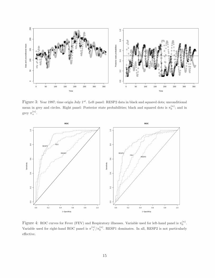
Figures 1–3 show our model’s approximation to the state and the stage of an epidemic curve.
The model was run on the 1997 data set for FEV, RESP1, and RESP2. On left-hand panel
of each graph, we display the unconditional mean Yn as stated in Theorem 1’ approximation
of the epidemic stage (grey), and the actual data values (black). The graphs on the left-hand
panel give graphical evidence that the unconditional mean Yn provides a good fit to the ob-
served readings. The right-hand panel displays two of the three posterior state probabilities.
Observe that the posterior probabilities change direction relative to changes in the epidemic
curve or with respect to changes in Yn. This suggests their reliability for sensitivity analysis,
provided they have an ease of predictability. This predictability is assessed in a ROC anal-
ysis. Figure 4. displays the ROC curves. The curves were built using π(n)0 as ROC variable
(left-hand panel) and on the right-hand panel using the posterior π(n)+ /π
(n)0 as a ROC crite-
rion. The ROC suggests that RESP1 unequivocally correlates better with influenza season
and is closely followed by FEV. It also is intuitively clear from both panels that RESP2
may not be the ideal prognostic factor. The low performance of RESP2 may be attributed
to the syndrome’ assessment; although tuning parameters may also have a say. Turning to
the ICD9 codes defining the syndrome, RESP2 is defined as other categories of respiratory
illnesses that cannot be clearly identified as RESP1; either known or unknown. This catego-
13
Page 14
rization becomes subjective by definition and invites more misclassification, irregularity and
more structural break than the clearly defined FEV and RESP1.
0 50 100 150 200 250 300 350
050
100
150
Time
Dat
a an
d U
ncon
ditio
nal m
ean
0 50 100 150 200 250 300 350
0.0
0.2
0.4
0.6
0.8
1.0
Time
Pos
terio
r st
ate
prob
abili
ties
Figure 1: Year 1997; time origin July 1st. Left panel: FEV data in black and squared dots; unconditional
mean in grey and circles. Right panel: Posterior state probabilities; black and squared dots is π(n)0 ; and in
grey π(n)+ .
0 50 100 150 200 250 300 350
010
020
030
040
050
060
0
Time
Dat
a an
d un
cond
ition
al m
ean
0 50 100 150 200 250 300 350
0.0
0.2
0.4
0.6
0.8
1.0
Time
Pos
terio
r st
ate
prob
abili
ties
Figure 2: Year 1997; time origin July 1st. Left panel: RESP1 data in black and squared dots; unconditional
mean in grey and circles. Right panel: Posterior state probabilities; black and squared dots is π(n)0 ; and in
grey π(n)+ .
14
Page 15
0 50 100 150 200 250 300 350
050
100
150
200
250
Time
Dat
a an
d un
cond
ition
al m
ean
0 50 100 150 200 250 300 350
0.0
0.2
0.4
0.6
0.8
1.0
Time
Pos
terio
r st
ate
prob
abili
ties
Figure 3: Year 1997; time origin July 1st. Left panel: RESP2 data in black and squared dots; unconditional
mean in grey and circles. Right panel: Posterior state probabilities; black and squared dots is π(n)0 ; and in
grey π(n)+ .
0.0 0.2 0.4 0.6 0.8 1.0
0.0
0.2
0.4
0.6
0.8
1.0
1−Specificity
Sen
sitiv
ity
RESP1FEV
RESP2
ROC
0.0 0.2 0.4 0.6 0.8 1.0
0.0
0.2
0.4
0.6
0.8
1.0
1−Specificity
Sen
sitiv
ity
RESP1FEV
RESP2
ROC
Figure 4: ROC curves for Fever (FEV) and Respiratory illnesses. Variable used for left-hand panel is π(n)0 .
Variable used for right-hand ROC panel is π(n)+ /π
(n)0 . RESP1 dominates. In all, RESP2 is not particularly
effective.
15
Page 16
The ROC analysis is particularly useful in finding a threshold value ~(π(n)• ) that yields the
‘best acceptable’ set of sensitivity and specificity. For example, with ~(π(n)0 ) = 0.42, RESP1
yields a sensitivity of 92.71% and a specificity of 72.59%. With the same threshold FEV
yields a sensitivity of 80.79% and a specificity of 73.55%. The value of ~(π(n)0 ) can be used
as threshold limit for a natural outbreak. Should one define a cost or utility function that
combines these two probability values, the ‘best acceptable’ threshold ~(π(n)0 ) may be chosen
to minimize this utility function. (See for example Metz, 1978; Pepe, 2003). To chart and
identify additional cases that could alter normal counts (e.g. in case of intentional release), it
is intuitive to keep a copy of the charting parameters (π(n)• ) under normal regime and assess
performance with respect to this baseline. In the absence of expert’s opinion to conduct a
full utility/cost analysis, we conduct a simulation study under normal regime to calibrate
a false alarm rate for charting. We run 1000 replications in which the observed FEV (or
RESP1) series is perturbed by normal fluctuation N(0, σ2). We assess false alarm relative
to the original true series through numerical optimization. To be explicit, if π(n)+ /π
(n)0 is the
ratio of the two posteriors under the true series, and π(n)+ /π
(n)0 |s is the corresponding value
in repeated iterations, we find a and b such that P (a < π(n)+ /π
(n)0 − π
(n)+ /π
(n)0 |s< b) = 1− α.
With a = −0.225 and b = 0.311, the false alarm rate is α = 0.002. This false alarm rate is
carried into the following simulated outbreaks study for signal detection.
4.2 Performance Under Different Outbreak Scenarios
Since the problem that spearheaded this research is outbreaks signal detection problem,
we simulated outbreaks in different ways that a pathogen could alter syndrome counts (see
Mandl et al., 2004 and Figure 8 in appendix B). The simulated outbreak extra cases are
superposed on the 1997 HDS and run through the developed model for signal detection. We
simulated outbreaks of one and two weeks. We spike the data stream with a number of indi-
vidual non-overlapping outbreaks. We space the outbreaks by 10, 20, and 30 days throughout
the year to ensure that seasonality in the data does not impede signal detection. We clean the
system before the next outbreak so that response to one outbreak does not carry over to the
next. The simulated data represents multiple ways in which pathogens could spread through
a community. Among the pathways considered, a flat outbreak corresponds to point-source
infections such as Bacillus Anthracis. Linear, exponential and sigmoid outbreaks may relate
to infectious diseases that are highly infectious, such as smallpox. Our working assumption
is that these outbreaks will reflect upon FEV and RESP1 (we discard RESP2 because of
its marginal performance in a ROC analysis). The number of simulated additional cases
16
Page 17
depends on the error profile of the agent under study (twice the standard deviation). Two
error profiles are considered; one for the flu season (winter) and one outside the flu season
(summer). The reasoning behind this is that visit rates vary more unpredictably in winter
than in summer. To illustrate, if the mean daily visit is 80 and the pathway gives a constant
error profile with standard deviation of 25, simulated outbreaks ranging from 0 to 50 extra
visits per day are considered. These visits are randomly sampled from 0 to 50 at a step of
5, and readjusted to fit the distributional pathway under study. In case the error profile
may vary between summer and winter, the number of additional cases may follow the season
accordingly, with more extra cases in winter. For example FEV has an error profile with
standard deviation 30 in winter and 22 otherwise.
4.2.1 Simulation Setting
We simulated one thousand (1,000) outbreaks for each of the following combinations: dura-
tion (7 days, 14 days), pathway (flat, linear, exponential, sigmoid), and yearly hit frequency
(once, twice). In case of more than one outbreak, the spacings used are 10, 20 or 30 days.
We kept a copy of the posterior ratio under normal regime and compared the simulated
performances to the normal for signal detection.
Here, we describe the basic idea behind generating a single outbreak. The idea carries
over to multiple non-overlapping outbreaks.
1. Choose a random n1 ∈ {1, . . . , 365−d} for the beginning of an outbreak with duration
d
2. Prior to n1 there is a normal course of an epidemic curve. Thus, the simulated data
before n1 is the original data 1, . . . , n1 − 1 plus a normal fluctuation N(0, σ2)
3. From time n1, generate an outbreak with duration d and pathway q. Add these out-
breaks to the original data stream plus a normal fluctuation
4. After time (n1 + d), the normal course continues; so, add normal fluctuation to the
original data set
5. Run the simulated data through the system for signal detection.
Figure 5 is an illustration of extra cases altering the normal FEV epidemic curve. For the
sake of clarity of the figure, we ignore the random fluctuations. This provides a pictorial
representation of how a single outbreak of duration d may look. In case of multiple epidemics,
17
Page 18
one may use spacing after step 4, then cycle back to step 1 and choose a restricted n1,2 >> n1.
It would also be wise to confine n1 to a time interval in case of multiple outbreaks.
0 50 100 150 200 250 300 350
050
100
150
200
Time
Dat
a an
d U
ncon
ditio
nal m
ean
0 50 100 150 200 250 300 350
050
100
150
200
Time
Dat
a an
d U
ncon
ditio
nal m
ean
Figure 5: Left-hand panel: Epidemic curve (grey) spiked with a seven-day flat outbreak at day 148 (black).
Right-hand panel: Epidemic curve (grey) spiked with a fifteen-day linear outbreak starting at day 122 (black).
Time origin is July 1st.
Assuming an outbreak was introduced at time n1 and that our system flags contamination
at time n2, we define the following measuring yardsticks:
• No Signal (N.S.) cases where the system is degenerate and fails to sound an alarm after
an outbreak has been introduced and during an outbreak
• Correct Signal (C.S.) cases where n2 = n1; to say that the system signals at the exact
time that an outbreak has been introduced
• Missed Signal (M.S.) cases where n2 > n1; to say that the system misses the exact
time but signals with delay
• False Signal (F.S.) cases where n2 < n1; to say that the system signals earlier than the
event has actually occurred (this has been set to have probability 0.002).
These partitions provide a tool for performance assessment under unusual activity. In
addition, a pictorial representation of signal and the missed signal compartments will help
display the delay to signal.
18
Page 19
4.2.2 Results of Sensitivity Analysis
Figures 6 – 7 provide a summary of the simulation results for single outbreaks. Among the
series that did not result in a F.S. prior to spiking the data stream with simulated outbreaks,
we evaluate the proportion of signal as well as the distribution of signals. Note that the flat
pathway and the linear result in the best detection of signal (see table 4 & 5). On the
tables, we display the cumulative signal detection as a numerical representation of the delay
to signal. Note that the seven-day flat picks out nearly all its signals two days after being
introduced (94.0%). The linear picks out nearly all its signals 3 days into spiking the data
stream (95.2%). The seven-day exponential and sigmoid have a slower reaction time. This
is to be expected because their shape starts out with low number of outbreaks then becomes
gradually increasing (see appendix B for a display of possible shapes). Some series failed to
signal during the outbreak period. We view those series as degenerate. Their proportions for
the seven-day outbreak follow: flat (1.2%) linear (1.6%), sigmoid (3.2%), and exponential
(2.8%). The proportion of degenerate series fades when the outbreak has a long duration
(see Table 5). The non-overlapping outbreaks simulation scenario yields similar results. This
is not a surprise because the system has been cleaned moving from the first to the second
outbreak.
% of Signal Day 1 Day 2 Day 3 Day 4 Day 5 Day 6 Day 7
Flat 79.6 92.4 94.0 96.0 97.2 98.4 98.8
Linear 29.2 71.2 91.2 95.2 97.2 98.0 98.4
Sigmoid 15.6 35.6 73.6 91.6 95.6 96.6 96.8
Exponential 07.2 16.4 38.8 71.2 87.6 95.6 97.2
Table 4: Table of cumulative signal for 7-day outbreaks. System set at a false alarm rate of 0.002
% of Signal Day 2 Day 4 Day 6 Day 8 Day 10 Day 12 Day 14
Flat 92.8 96.8 97.6 98.0 99.2 99.2 100
Linear 37.2 87.2 96.4 98.0 98.4 99.6 100
Sigmoid 08.0 14.4 23.6 47.2 88.8 98.8 100
Exponential 12.8 20.8 27.6 32.4 62.8 94.8 99.2
Table 5: Table of cumulative signal for 14-day outbreaks. System set at a false alarm rate of 0.002
19
Page 20
Performance
Days
Fre
quen
cy
1 2 3 4 5 6 7
020
040
060
080
0
Performance
Days
Fre
quen
cy
1 2 3 4 5 6 7
010
020
030
040
0
Performance
Days
Fre
quen
cy
1 2 3 4 5 6 7
050
100
150
200
250
300
Performance
Days
Fre
quen
cy
1 2 3 4 5 6
010
020
030
0
Figure 6: Performance on 7-day outbreaks. Top row: Flat and linear Linear. Bottom row: Exponential
and Sigmoid.
5 Simulation Comparative Study
Since part of our goal is to build a control algorithm with the potential of identifying clusters
of disease cases before traditional methods, we use the decision interval Cusum on the first
difference readings following the 7-day rolling window filtration. The reason for using the
Cusum on the first difference spurred from the fact that first differences have a tendency
to remove bias from series and leave them with noise. After all, the readings have to be
detrended/demodulated for the Cusum to reach its optimality. Next, the first differences are
20
Page 21
Performance
Days
Fre
quen
cy
2 4 6 8 10 12 14
020
040
060
080
0
Performance
Days
Fre
quen
cy
2 4 6 8 10 12 14
010
020
030
0
Performance
Days
Fre
quen
cy
2 4 6 8 10 12
050
100
150
200
Performance
Days
Fre
quen
cy
2 4 6 8 10 12 14
050
100
150
200
Figure 7: Performance on 14-day outbreaks: Top row: Flat and linear Linear. Bottom row: Exponential
and Sigmoid.
transformed to achieve normality. Our approach builds 2 Cusums for shift in the mean; one
upward and one downward. We run these Cusums until one crosses its decision interval, so
that the out of control run length is the minimum of the two. We compare this first-signal-
based Cusum to the performance of the Bayesian approach. To be fair, the comparison is
plausible on one ground only: the flat outbreak pathway. The reason is that optimality of a
Cusum holds from one step change to another step change; not from step to gradual changes.
It would have been a clear disadvantage for the Cusum if the comparison were carried for
outbreaks with gradual pathway. Speaking of the Cusum design, in order to obtain a joint
21
Page 22
in-control ARL of 500, we must tune each individual Cusum at a nominal ARL of 1000.
The in-control ARL was matched by the performance of the Bayesian method under normal
operation resulting in a false alarm rate of 0.002 (see Montgomery 2009, Hawkins and Olwel
1998). Since we used 2-year observations to elicit the Bayesian model parameters, the same
number of observations is used to calibrate our Cusums. The filtered and demodulated
HDS is N(0.02, 4.71); which needed another standardization. The reference value and the
decision intervals for the Cusums depend on the shift we anticipate to detect. In our case,
with reference value of 1 for an upward shift, -1 for a downward shift, and a decision interval
of 2.6666, both Cusums are tuned to detect 2 standard deviation shifts from a N(0,1) error
profile and attain an average run length of 1000 each. We run 1000 of contaminated series
through both the Bayesian model and through the Cusum; and we recorded the proportion
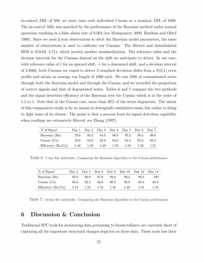
of correct signals and that of degenerated series. Tables 6 and 7 compare the two methods
and the signal detection efficiency of the Bayesian over the Cusum–which is in the order of
1.5 to 1. Note that in the Cusum case, more than 30% of the series degenerate. The intent
of this comparative study is by no means to downgrade cumulative sums; but rather to bring
to light some of its abuses. The point is that a process loses its signal detection capability
when readings are extensively filtered; see Zhang (1997).
% of Signal Day 1 Day 2 Day 3 Day 4 Day 5 Day 6 Day 7
Bayesian (Ba) 79.6 92.4 94.0 96.0 97.2 98.4 98.8
Cusum (Cu) 53.6 62.0 62.8 63.6 64.4 65.2 65.2
Efficiency (Ba/Cu) 1.48 1.49 1.49 1.50 1.50 1.50 1.51
Table 6: 7-day flat outbreaks. Comparing the Bayesian algorithm to the Cusum performance
% of Signal Day 2 Day 4 Day 6 Day 8 Day 10 Day 12 Day 14
Bayesian (Ba) 92.8 96.8 97.6 98.0 99.2 99.2 100
Cusum (Cu) 60.0 62.4 63.6 66.0 66.8 68.4 68.8
Efficiency (Ba/Cu) 1.54 1.55 1.53 1.48 1.48 1.45 1.45
Table 7: 14-day flat outbreaks. Comparing the Bayesian algorithm to the Cusum performance
6 Discussion & Conclusion
Traditional SPC tools for monitoring data pertaining to biosurveillance are currently short of
capturing all the important structural changes depicted on these data. These tools lose their
22
Page 23
performance due to the background of variability seen on biosurveillance data. We have de-
veloped a three-state sequential and recursive algorithm that accounts for some of the issues
encountered in biosurveillance. The algorithm is bayesian and accounts for non-stationarity,
irregularity, and seasonality through sequentially updated prior distribution parameters. Our
approach has the added advantage to adjust to random jumps, both in magnitude and in
direction, and to capture an epidemic curve serial structural details. Compared to Cusum
on simulated flat outbreaks, its efficiency is 1.5 to 1.
Other approaches based on Hidden Markov Models (HMM) and Markov Switching Mod-
els (MSM) are also used in conjunction with epidemiological types of data. Within this
framework, an unobserved epidemic state space is modeled using homogeneous Markov chain
of order one (1) with stationary transition probabilities (see for example Le Strat et al.,
1999, for HMM and Lu et al., 2010, for MSM; see also Cappe, et al., 2007 and Fruehwirth-
Schnatter, 2006 for statistical developments in HMM and MSM models). These methods are
usually computationally intensive with a questionable performance in start-up settings when
only a short history is available at the beginning of a monitoring scheme. Also, multivariate
methods may be worth exploring when many syndromic variables are under study. This
issue needs more space and mathematical development than can be devoted to it here. Mul-
tivariate case charts are not assumption-free and are more demanding in their calibration
needs than univariates’. A reasonable multivariate development would consist of using some
syndromic variables in a ‘strength borrowing’ fashion to monitor the remaining incidence
parameters.
The current proposal will augment early reports of natural epidemics or intentional oper-
ations to sentinels. Its novelty comes from monitoring the states posterior probabilities and
from its self-reliance. We view our proposal as a self-reliant method, with the potential to
combine three different aspects of control theory into a single process: modeling, charting,
and forecasting. We also recognize that our proposal is not ‘one size fits all’. Biosurveillance
data may differ from one location to another in the same country. As one switches from
location to location or between syndromic variables, the general philosophy behind our pro-
posal holds; but parameters may change. Thus, the need to re-tune some parameters and
reset some initial values.
23
Page 24
7 Technical Appendix–A
The theorem is proved by induction. For n = 1 it is easy to show that the theorem holds.
Specifically, the unconditional distribution of Y1 is a mixture of 3 Normal distributions:
f(Yn) =2∑
i=0
w(1)i N
(µ
(1)i ,
(σ
(1)i
)2)
where for the weights, means and variances, we have:
w(1)0 = π
(0)0 µ
(1)0 = λζ
(σ
(1)0
)2
= σ2 + λ2σ20
w(1)1 = π
(0)− µ
(1)1 = λζ −∆
(σ
(1)1
)2
= τ 2 + σ2 + λ2σ20
w(1)2 = π
(0)+ µ
(1)2 = λζ + ∆
(σ
(1)2
)2
= τ 2 + σ2 + λ2σ20 .
For the posterior probabilities of the events Ei we have:
P (E1 = 0|Y1 = y1) =
2∑i=0
π(0)0√
2π[σ2+λ2σ20]
exp
{− (y1−λζ)2
2[σ2+λ2σ20]
}
f(Y1 = y1)= π
(1)0 ,
P (E1 = −1|Y1 = y1) =
2∑i=0
π(0)−√
2π[τ2+σ2+λ2σ20]
exp
{− (y1−[λζ−∆])2
2[τ2+σ2+λ2σ20]
}
f(Y1 = y1)= π
(1)− , and
P (E1 = +1|Y1 = y1) =
2∑i=0
π(0)+√
2π[τ2+σ2+λ2σ20]
exp
{− (y1−[λζ+∆])2
2[τ2+σ2+λ2σ20]
}
f(Y1 = y1)= π
(1)+ .
Next, assume that the theorem holds for n − 1; i.e. the unconditional distribution of Yn−1
given by
f(Yn−1) =3n−1−1∑
i=0
w(n−1)i N
(µ
(n−1)i ,
(σ
(n−1)i
)2)
,
where for the weights, means, variances, and the posterior probabilities of the events Ei, the
recursive relationships are valid. Then, we can show that it is valid for n. Indeed,
Yn|Yn−1, δ, En ∼ N(λYn−1 + Enδ, σ2
)
Yn−1 ∼3n−1−1∑
i=0
w(n−1)i N
(µ
(n−1)i ,
(σ
(n−1)i
)2)
δ ∼ N(∆, τ 2
).
24
Page 25
From the above we obtain the distribution of Yn|En:
Yn|En ∼3n−1−1∑
i=0
w(n−1)i N
(λµ
(n−1)i + En∆, E2
nτ 2 + σ2 + λ2(σ
(n−1)i
)2)
En =
0 with prob. π(n−1)0
−1 with prob. π(n−1)−
+1 with prob. π(n−1)+
.
Then for the unconditional distribution of Yn we have:
Yn ∼3n−1−1∑
i=0
[w
(n−1)i π
(n−1)0 N
(λµ
(n−1)i , σ2 + λ2
(σ
(n−1)i
)2)
+ w(n−1)i π
(n−1)− N
(λµ
(n−1)i −∆, τ 2 + σ2 + λ2
(σ
(n−1)i
)2)
+ w(n−1)i π
(n−1)+ N
(λµ
(n−1)i + ∆, τ 2 + σ2 + λ2
(σ
(n−1)i
)2)]
≡3n−1∑i=0
w(n)i N
(µ
(n)i ,
(σ
(n)i
)2)
;
which satisfies the recursive relationships for the weights, means and variances. Furthermore,
for the posterior distribution of En we get:
P (En = 0|Yn = yn) =
3n−1−1∑i=0
w(n−1)i
π(n−1)0√
2π
[σ2+λ2
(σ
(n−1)i
)2]exp
{−
(yn−λµ
(n−1)i
)2
2
[σ2+λ2
(σ
(n−1)i
)2]
}
f(Yn = yn)= π
(n)0 ,
P (En = −1|Yn = yn) =
3n−1−1∑i=0
w(n−1)i
π(n−1)−√
2π
[τ2+σ2+λ2
(σ
(n−1)i
)2]exp
{−
(yn−
[λµ
(n−1)i
−∆])2
2
[τ2+σ2+λ2
(σ
(n−1)i
)2]
}
f(Yn = yn)= π
(n)− ,
P (En = +1|Yn = yn) =
3n−1−1∑i=0
w(n−1)i
π(n−1)+√
2π
[τ2+σ2+λ2
(σ
(n−1)i
)2]exp
{−
(yn−
[λµ
(n−1)i
+∆])2
2
[τ2+σ2+λ2
(σ
(n−1)i
)2]
}
f(Yn = yn)= π
(n)+ ;
which are consistent with the formulas provided in the theorem.
Bounds on the parameters of f(Yn) :
Here, we establish the proof that the means, variances and weights are bounded.
25
Page 26
Means
The lowest (highest) possible mean corresponds to the case where we have a negative (posi-
tive) jump at each of the n stages of the process. Using induction one has:
µ(n)min = λnζ − λn−1∆− λn−2∆− . . .− λ∆−∆
= λnζ −(
1− λn
1− λ
)∆,
µ(n)max = λnζ + λn−1∆ + λn−2∆ + . . . + λ∆ + ∆
= λnζ +
(1− λn
1− λ
)∆.
Thus at each stage n of the process all 3n means are bounded in
[µ
(n)min, µ
(n)min
]=
[λnζ −
(1− λn
1− λ
)∆, λnζ +
(1− λn
1− λ
)∆
],
with range converging as follow:
2
(1− λn
1− λ
)∆
n↑−→ 2∆
1− λ.
As n grows, these means are within the range of at most 2∆/(1−λ), leading to the conclusion
that they become less and less different from each other as n increases.
Variances
The two most extreme scenarios for the variances are:(σ
(n)min
)2
: corresponding to a no-jump state for all n stages of the process(σ
(n)max
)2
: corresponding to all-jump states (positive or negative) for all n stages of the
process. Based on the recursion we can easily show:
(σ
(n)min
)2
= σ2 + λ2σ2 + λ4σ2 + . . . + λ2n−2σ2 + λ2nσ20
= λ2nσ20 +
(1− λ2n
1− λ2
)σ2,
(σ
(n)max
)2
=(σ2 + τ 2
)+ λ2
(σ2 + τ 2
)+ λ4
(σ2 + τ 2
)+ . . . + λ2n−2
(σ2 + τ 2
)+ λ2nσ2
0
= λ2nσ20 +
(1− λ2n
1− λ2
) (σ2 + τ 2
).
At each stage n of the process all 3n variance terms are bounded in
[(σ
(n)min
)2
,(σ
(n)max
)2]
=
[λ2nσ2
0 +
(1− λ2n
1− λ2
)σ2, λ2nσ2
0 +
(1− λ2n
1− λ2
) (σ2 + τ 2
)],
26
Page 27
with range converging as follow:
(1− λ2n
1− λ2
)τ 2 n↑−→ τ 2
1− λ2.
As n increases the variance terms become similar.
Weights
The weights involve a non-linear relation between the posterior probabilities and the data
readings. An exact mathematical bound on these entities in not a reasonable task. However,
given that the weights fall in [0,1] and add up to 1, as n increases all 3n weights become
smaller. Based on the recursive relationship at each stage n of the process the weights of the
previous stage n− 1 are multiplied with the respective posterior probabilities (i.e. a number
in [0,1]) making them smaller.
Technical Appendix–B
Flat
0.00
0.04
0.08
0.12
Linear
0.00
0.10
0.20
Exponential
0.0
0.1
0.2
0.3
0.4
0.5
Sigmoid
0.00
0.05
0.10
0.15
0.20
Figure 8: Various shapes of outbreaks considered. These are canonical frequency shapes for display; random
displacements have not been added to them yet; the span of each outbreak is 7 days.
27
Page 28
FEV: Includes febrile illnesses of unspecified origin, unknown viral illnesses accompanied by
fever, fever and septicemia not specified.
RESP: Includes any acute infection of the upper and/or lower respiratory tract (from the
oropharynx to the lungs, includes otitis media), diagnosis of acute respiratory tract infection
such as pneumonia due to parainfluenza virus, acute non-specific diagnosis of respiratory
tract infection such as sinusitis, pharyngitis, laryngitis, cough, stridor, shortness of breath,
and throat pain. Exclude chronic bronchitis, allergic conditions and asthma. These respi-
ratory diagnoses are believed to be linked to anthrax (inhalational) , tularemia and plague
(pneumonic).
RESP1: Reflects general symptoms of respiratory illnesses and also includes associated
bioterrorism diseases of highest concern or diseases highly approximating them.
RESP2: Consists of symptoms that might normally be placed in respiratory illness group
but daily volume could detract from the signal generated by RESP1.
8 Reference
Arnon S.S., Schechter R., Inglesby T.V., 2001. Tulinum toxin as a biological weapon:
medical and public health management. Journal of the American Medical Association.
285, 1059–70.
Berger, J.O., 1980. Statistical Decision Theory; Foundation, Concept and Methods,
Springer Verlag, New York.
Bloomfiled, P., 1976. Fourier Analysis for Time Series: An Introduction, Wiley, New
York.
Buehler J.W., Berkelman R.L., Hartley D.M., Peters C.J., 2003. Syndromic surveil-
lance and bioterrorism-related epidemics. Emerging Infectious Diseases. 9, 1197-1204.
Cappe, O., Moulines, E., Ryden, T., 2007. Inference in Hidden Markov Models,
Springer Series in Statistics, Springer, New York.
Casella, G., Berger, R. L., 1990. Statistical Inference, Wadsworth & Brooks-Cole,
Pacific Grove, California.
28
Page 29
Center for Disease Control and Prevention, MMWR 2001. Recognition of Illness Asso-
ciated with the Intentional Release of a Biologic Agent. MMWR, 10.19.2001, 50(41),
893- 897.
De Groot, M.H., 1970. Optimal Statistical Decision, McGraw-Hill, New York.
Dennis D.T., Inglesby T.V., Henderson D.A., 2001. Tularemia as a biological weapon:
medical and public health management. Journal of the American Medical Association.
285, 2763–73.
Fruhwirth-Schnatter, S., 2006. Finite Mixture and Markov Switching Models, Springer
Series in Statistics, Springer, New York.
Geisser, S., 1993. Predictive Inference: An Introduction, Chapman & Hall, London.
Green M.S., Kaufman Z., 2002. Surveillance for early detection and monitoring of
infection disease outbreaks associated with bioterrorism. Israel Medical Association
Journal. 4(7), 503-6.
Hawkins, D.M., Olwell, D.H., 1998. Cumulative Sum Charts and Charting for Quality
Improvement, Springer Verlag, New York.
Hawkins, D.M., Qiu, P., Kang, C.W., 2003. The Change point Model for Statistical
Process Control. Journal of Quality Technology. 35, 355-365.
Hawkins, D.M., Zamba, K.D., 2005a. A Change point Model for Statistical Process
Control with Shift in mean or Variance. Technometrics. 47(2), 164-173.
Hawkins, D.M., Zamba, K.D., 2005b. Change point Model for a Shift in Variance.
Journal of Quality Technology. 37(1), 21-31.
Henderson D.A., Inglesby T.V., Bartlett J.G., 1999. Smallpox as a biological weapon:
medical and public health management. Journal of the American Medical Association.
281, 2127–37.
Hutwagner L.C., Maloney E.K., Bean N.H., Slutsker L., Martin S.M., 1997. Using
Laboratory-based Surveillance data for Prevention: An algorithm to detect Salmonella
Outbreaks. Emerging Infectious disease. 3, 395-400.
Jeffreys, H., 1948. Theory of Probability, Second Edition, University Press, Oxford.
29
Page 30
Inglesby T.V., Henderson D.A., Bartlett J.G., 1999. Anthrax as a biological weapon:
medical and public health management. Journal of the American Medical Association.
281, 1735.
Inglesby T.V., Dennis D.T., Henderson D.A., 2000. Plague as a biological weapon:
medical and public health management. Journal of the American Medical Association.
283, 2281–2290.
Le Strat, Y., Carrat, F., 1999. Monitoring epidemiologic surveillance data using hidden
Markov models. Statistics in Medicine. 18, 34633478.
Lotze, T., Murphy, S., Shmueli, G., 2008. Implementation and Comparison of Pre-
processing Methods for Biosurveillance Data. Advances in Disease Surveillance. 6(1),
1-20.
Lu, H.-M., Zeng, D., Chen, H., 2010. Prospective infectious disease outbreak detection
using Markov switching models. IEEE Transactions on Knowledge & Data Engineer-
ing. 22, 565577.
Mandl, K.D., Reis, B., Cassa, C., 2004. Measuring Outbreak–Detection Performance
by Using Controlled Feature Set Simulations. Morbidity and Mortality Weekly Report
(MMWR). 53, 130–136.
McLachlan, G.J., Basford, K.E., 1988. Mixture Models Inference and Applications to
Clustering, Marcel Dekker, New York.
Metz, C.E., 1978. Basic Principle of ROC Analysis. Seminars in Nuclear Medicine. 8,
283–298.
Montgomery, D.C., 2009. Introduction to Statistical Quality Control, John Wiley and
Son, New York.
Pavlin J.A., 2003. Investigation of Disease Outbreaks Detected by Syndromic Surveil-
lance Systems. Journal of Urban Health. 80, 107-114.
Pepe, M.S., 2003. The Statistical Evaluation of Medical Tests for Classification and
Prediction, University Press, Oxford.
Shmueli, G., Burkom, H.S., 2010. Statistical Challenges Facing Early Outbreak De-
tection in Biosurveillance. Technometrics (Special Issue Anomaly Detection). 52(1),
39-51.
30
Page 31
Stern, L., Lightfoot D., 1999. Automated outbreak detection: A Quantitative Retro-
spective Analysis. Epidemiology of Infectious disease. 122, 103-110.
Stoto M.A., Schonlau M., Mariano L.T., 2004. Syndromic Surveillance: Is it Worth
the Effort?. Chance. 17(1), 19-24.
Tsiamyrtzis, P., Hawkins, D.M., 2010. Bayesian Start up Phase Mean Monitoring of
an Autocorrelated Process that is Subject to Random Sized Jumps. Technometrics.
52(4), 438-452.
West, M., 1993. Approximating posterior distributions by Mixtures. Journal of Royal
Statistical Society, Series B. 55, 2, 409-422.
Winkel, P., Zhang, N.F., 2007. Statistical Development of Quality in Medicine, John
Wiley & Sons Ltd, England.
Woodall, W.H., 2006. The Use of Control Charts in Health-Care and Public-Health
Surveillance. Journal of Quality Technology. 38(2), 89–104.
Zamba, K.D., Tsiamyrtzis, P., Hawkins, D.M., 2008. A Sequential Bayesian Con-
trol Model for Influenza-Like Illnesses and Early Detection of Intentional Outbreaks.
Quality Engineering. 20(4) 495-507.
Zhang, N.F., 1997. Detection capability of residual control chart for stationary process
data. Journal of Applied Statistics. 24, 475-492.
31