A Timoshenko beam theory with pressure corrections for

layered orthotropic beams

Graeme J. Kennedya,1,∗, Jorn S. Hansena,2, Joaquim R.R.A. Martinsb,3

aUniversity of Toronto Institute for Aerospace Studies, 4925 Dufferin Street, Toronto, M3H 5T6,

CanadabDepartment of Aerospace Engineering, University of Michigan, Ann Arbor, MI 48109, USA

Abstract

A Timoshenko beam theory for layered orthotropic beams is presented. The theoryconsists of a novel combination of three key components: average displacement androtation variables that provide the kinematic description of the beam, stress and strainmoments used to represent the average stress and strain state in the beam, and the useof exact axially-invariant plane stress solutions to calibrate the relationships betweenall these quantities. These axially-invariant solutions, which we call the fundamentalstates, are also used to determine a shear strain correction factor as well as correctionsto account for effects produced by externally-applied loads. The shear strain correctionfactor and the external load corrections are computed for a beam composed of isotropiclayers. The proposed theory yields Cowper’s shear correction for a single isotropic layer,while for multiple layers new expressions for the shear correction factor are obtained.A body-force correction is shown to account for the difference between Cowper’s shearcorrection and the factor originally proposed by Timoshenko. Numerical comparisonsbetween the theory and finite-elements results show good agreement.

Keywords: Timoshenko beam theory, shear correction factor

1. Introduction

The equations of motion for a deep beam that include the effects of shear deformationand rotary inertia were first derived by Timoshenko (1921, 1922). Two essential aspects ofTimoshenko’s beam theory are the treatment of shear deformation by the introduction ofa mid-plane rotation variable, and the use of a shear correction factor. The definition andvalue of the shear correction factor have been the subject of numerous research papers,some of which are discussed below. Shames and Dym (1985, Ch. 4, pg. 197) provide

∗Corresponding authorEmail addresses: graeme.kennedy@utoronto.ca (Graeme J. Kennedy), hansen@utias.utoronto.ca

(Jorn S. Hansen), jrram@umich.edu (Joaquim R.R.A. Martins)1PhD Candidate2Professor Emeritus3Associate Professor

Preprint submitted to Elsevier November 30, 2011

an excellent overview of the classical approach to Timoshenko beam theory. This paperhowever, draws primarily from research and theories which refine Timoshenko’s originalapproximations.

Prescott (1942) derived the equations of vibration for thin rods using average through-thickness displacement and average rotation variables. He introduced a shear correctionfactor to account for the difference between the average shear on a cross section and theexpected quadratic distribution of shear.

Cowper (1966) presented a revised derivation of Timoshenko’s beam theory startingfrom the equations of linear elasticity for a prismatic, isotropic beam in static equilibrium.Cowper introduced residual displacement terms that he defined as the difference betweenthe actual displacement in the beam and the average displacement representation. Theseresidual displacements account for the difference between the average shear strain andthe shear strain distribution. Cowper introduced a correction factor to account for thisdifference and computed its value based on the three-dimensional solution of a cantileverbeam subjected to a tip load.

Stephen and Levinson (1979), developed a beam theory along the lines of Cowper’s,but recognized that the variation in shear along the length of the beam would lead to amodification of the relationship between bending moment and rotation. This variationhad been neglected by Cowper.

Following the work of Cowper (1966) and Stephen and Levinson (1979), in this paperwe seek a solution to a beam problem based on average through-thickness displacementand rotation variables. In a departure from previous work, we introduce strain mo-

ments, which are analogous to the stress moments used in the equilibrium equations.These strain moments remove the restriction of working with an isotropic, homoge-neous beam. This is an essential component of the present approach, as sandwich andlayered orthotropic beams are often used for high-performance, aerospace applications(Flower and Soutis, 2003).

Another important feature of our theory is the use of certain statically determinatebeam problems that we use to construct the relationship between stress and strain mo-ments, and to reconstruct the stress and strain solution in a post-processing step. Wecall these solutions the fundamental states of the beam. The present theory was firstpursued by Hansen and Almeidia (2001) and Hansen et al. (2005), and an extension ofthis theory to the analysis of plates was presented by Guiamatsia and Hansen (2004),Tafeuvoukeng (2007) and Guiamatsia (2010).

This paper begins with a brief discussion of two classical methods used to calculatethe shear correction factor in Section (2). Section (3) describes the proposed theoryand Section (3.2) introduces the fundamental states. In Section (4), calculations arepresented for a beam composed of multiple isotropic layers. Section (5) briefly presentsthe modified equations of motion for an isotropic beam. In Section (6), comparisonsare made with finite-element calculations. Section (7) outlines conclusions based on thetheory presented herein.

2. The shear correction factor

One of the main difficulties in using Timoshenko beam theory is the proper selectionof the shear correction factor. Many authors have published definitions of the shear

2

correction factor and have proposed various methods to calculate it. Most of theseapproaches fall into one of two categories. The first approach is to use the shear correctionfactor to match the frequencies of vibration of various beam constructions with exactsolutions to the theory of elasticity. The second approach is to use the shear correctionfactor to account for the difference between the average shear or shear strain and theactual shear or shear strain using exact solutions to the theory of elasticity.

Timoshenko (1922) developed the frequency-matching approach. He calculated theshear correction factor by equating the frequency of vibration determined using the planestress equations of elasticity to those computed using his beam theory. Although notexplicitly written in the paper, the shear correction factor obtained in this manner for arectangular beam is

kxy =5(1 + ν)

6 + 5ν. (1)

Cowper (1966) calculated the shear correction factor using an approach from thesecond category described above. Using residual displacements designed to take intoaccount the distortion of the cross sections under shear loads, Cowper was able to derivea formula for the shear correction factor based on solutions of a cantilever beam subjectedto a tip load. For a rectangular isotropic homogeneous beam, Cowper found the followingshear correction factor:

kxy =10(1 + ν)

12 + 11ν. (2)

Following Cowper’s approach, Stephen (1980) computed the shear correction factorfor beams of various cross sections by using the exact solutions for a beam subjectto a uniform gravity load. He employed a modified form of the Kennard–Leibowitzmethod (Leibowitz and Kennard, 1961), to obtain the shear correction factor by equatingthe average centerline curvature of the exact result with the Timoshenko solution. Heobtained a modified form of Timoshenko’s shear correction factor for rectangular sectionsthat approached Equation (1) for thin cross-sections.

Using the frequency matching approach, Hutchinson (1981) computed the shear cor-rection factor by performing a comparison between Timoshenko beam theory and threesolutions from the theory of elasticity, the Pochhammer–Chree solution in Love (1920),a Fourier solution due to Pickett (1944) and a series solution computed by Hutchinson(1980). Hutchinson found that the best shear correction factor was dependent on thefrequency and Poisson’s ratio of the beam, but that Timoshenko’s value was better thanCowper’s.

Later, Hutchinson (2001) introduced a new Timoshenko beam formulation and com-puted the shear correction factor for various cross sections based on a comparison witha tip-loaded cantilever beam. For a beam with a rectangular cross section, Hutchinsonobtained a shear correction factor that depends on the Poisson ratio and the width todepth ratio. In a later discussion of the paper, Stephen (2001) showed that the shearcorrection factors he obtained in Stephen (1980) were equivalent.

More recently Dong et al. (2010), presented a semi-analytic finite-element techniquefor calculating the shear correction factor based either on the Saint–Venant warpingfunction or the free vibration of a beam.

Some experimental studies have been performed to try and measure the shear correc-tion factor based on the original equations proposed by Timoshenko. Spence and Seldin

3

(1970) obtained experimental values of the shear correction factor for a series of squareand circular beams composed of both isotropic and anisotropic materials by determiningtheir natural frequencies. Kaneko (1975) performed an extensive review of the shearcorrection factors for rectangular and circular cross sections obtained by various authorsusing either experimental techniques or analysis. Experimental studies have generallyused a natural frequency approach to determine the shear correction factor and havegenerally found that Timoshenko’s value is superior to Cowper’s. This is perhaps notsurprising, since Timoshenko’s correction was obtained by matching frequencies in thesame manner in which the experiments are performed. However, the frequency matchingapproach fails to provide a theoretical explanation as to why the value of a factor thatmodifies the relationship between the shear resultant and the average shear strain shouldbe determined by the natural frequency of vibration. It is this deficiency that motivatesthe work presented here.

2c

y

z

1

y

x

L

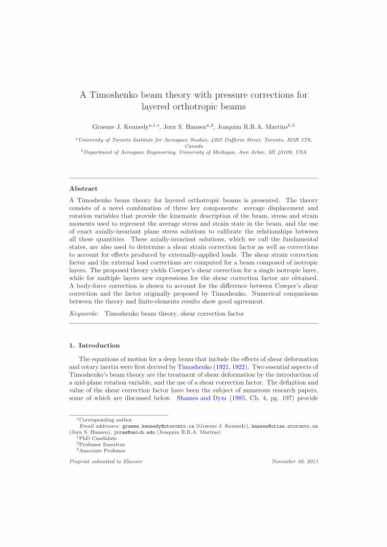
Figure 1: The geometry of the beam composed of layers of different materials.

3. The theory

The geometry of the beam under consideration is shown in Figure 1. The beamextends along the x-direction subject to forces on the top and bottom surfaces in they-direction. The reference axis is placed at the centroid of the cross-section. The half-thickness in the y-direction is c, while the length of the beam in the x-direction is L. Thebeam is of uniform composition in both the x and z-directions and so consists of a seriesof layers with different material properties. We assume that each layer is composed of anorthotropic material, with material properties aligned with the coordinate axes. Theseassumptions eliminate the possibility of twisting and allow the beam to be modeled usinga plane stress assumption in the z plane. In each layer k, numbered from the bottom tothe top of the beam, the following constitutive law holds:

σ(k) = C(k)ǫ(k),

where σ(k) =[

σx σy σxy

]T

(k)and ǫ(k) =

[

ǫx ǫy γxy]T

(k). Since the beam is

composed of an orthotropic material, there is no coupling between shear and normalstresses. Although variation in the Poisson’s ratio between layers would lead to a violationof the plane stress assumption, we include this possibility and ignore the edge effects inthe cross-section in such situations.

4

These assumptions are an extension of the conditions originally used by Timoshenko,who limited his analysis to plane stress beams composed of a single isotropic mate-rial (Timoshenko, 1922).

3.1. The displacement representation

Following Prescott (1942) and Cowper (1966), the average through-thickness displace-ments and average rotation are defined as follows:

u0(x, t) =1

2c

∫ c

−c

u(x, y, t) dy,

u1(x, t) =3

2c3

∫ c

−c

yu(x, y, t) dy,

v0(x, t) =1

2c

∫ c

−c

v(x, y, t) dy,

(3)

where u and v are the displacements in the x and y directions, respectively. The averagedisplacements and rotation are defined regardless of the through-thickness behavior of uand v, which are piecewise continuous through the thickness of the beam in this problem.The average displacements are an incomplete representation of the total displacementfield in the beam, in the sense that the average quantities do not capture the point-wisebehavior of the exact displacement. In order to capture this behavior, it is necessary tointroduce residual displacements that account for the difference between the average andpoint-wise quantities in the following manner:

u(x, y, t) = u0(x, t) + yu1(x, t) + u(x, y, t),

v(x, y, t) = v0(x, t) + v(x, y, t),(4)

where u and v are the residual displacements in the x and y directions, as introduced byCowper (1966). Given the definitions of the average displacements (3), the zeroth andfirst moments of u, and the zeroth moment of v through the thickness, must be zero:

∫ c

−c

u(x, y, t) dy = 0,

∫ c

−c

yu(x, y, t) dy = 0,

∫ c

−c

v(x, y, t) dy = 0.

The average displacements and displacement residuals may be used to determine thestrain at any point in the beam. In this approach however, we are interested in the averagethrough-thickness strain. To this end, we introduce the following strain moments:

ǫ0(x, t) =

∫ c

−c

∂u

∂xdy = 2c

∂u0

∂x, (5a)

κ(x, t) =

∫ c

−c

y∂u

∂xdy =

2c3

3

∂u1

∂x, (5b)

γ(x, t) =

∫ c

−c

[

∂u

∂y+

∂v

∂x

]

dy = 2c

[

u1 +∂v0∂x

]

+

∫ c

−c

∂u

∂ydy, (5c)

5

that represent the axial, bending and shear strain moments, respectively. These strainmoments are analogous to the stress moments that are used to define the equilibriumequations for a beam. Note that these strain moments are not normalized and as a re-sult have different dimensions than the point-wise strain. The main advantage of usingthe strain moments (5) over point-wise strain variables is that they are always defined,regardless of the through-thickness distribution of the strain. This is an important prop-erty, since the point-wise shear strain can be discontinuous at material interfaces.

Thus far, no assumptions beyond those of linear elasticity have been made. Thecombination of the average and residual displacements can be used to capture an arbitrarydisplacement field. Next, we examine the state of stress within the beam.

3.2. The fundamental states

The basic assumption made in the development of the present beam theory is thatthe stress and strain state in the beam can be approximated using a linear combinationof axially-invariant solutions. We call these axially-invariant solutions the fundamental

states. The fundamental states can be used to capture the complex interaction betweenthe stresses in layered orthotropic beams, away from the ends of the beam. As is thecase in many beam theories, end effects cannot be captured using this approach. In thissection we address how to determine the fundamental states.

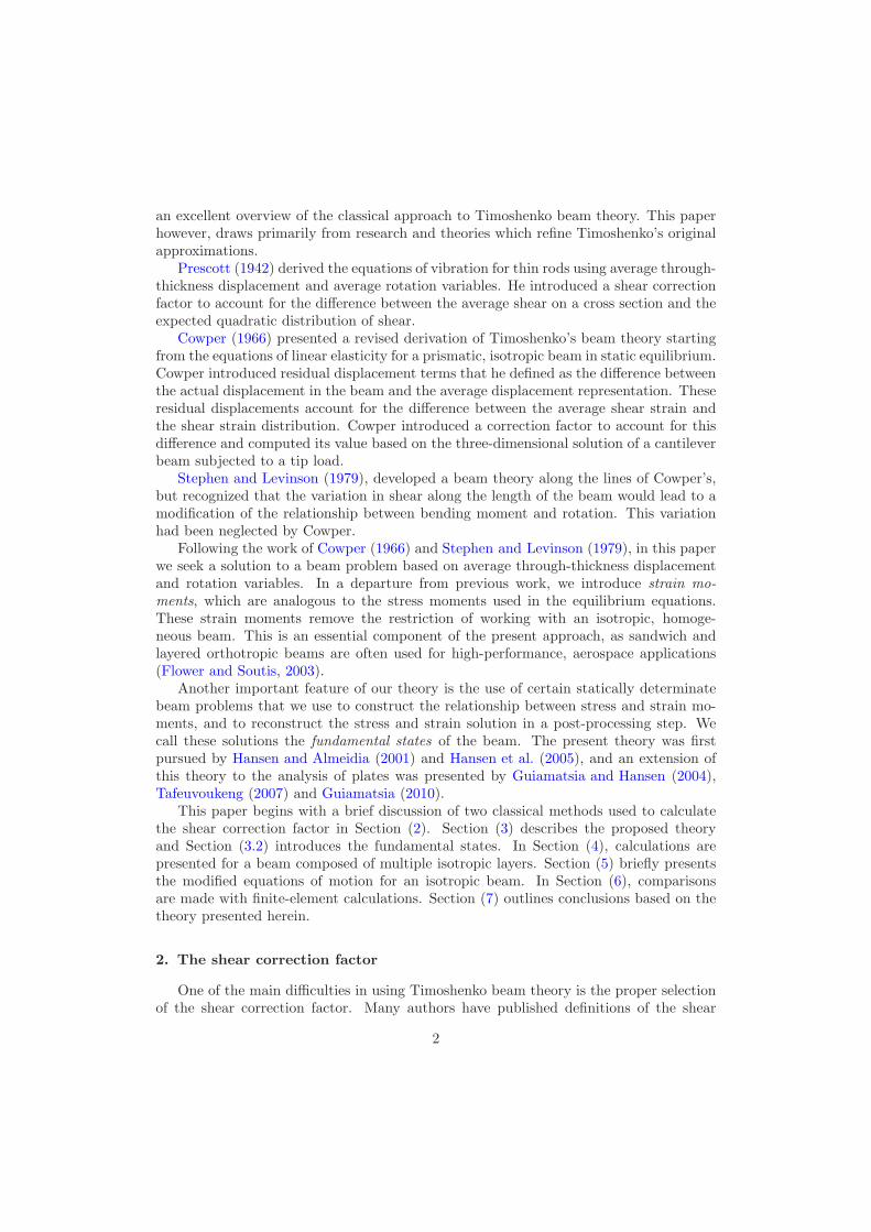
The fundamental states are determined from a hierarchy of statically determinatebeam problems. These beam problems are formulated using a series of self-equilibratingloads applied to a beam with the same sectional properties as the beam under consid-eration. Rigid body translation and rotation modes are removed from the solution byimposing three displacement constraints so that no stress concentrations are present.The first four loading conditions leading to the first four fundamental states are shownin Figure 2. N , M and Q are the axial, bending, and shear resultants, defined as follows:

N(x, t) =

∫ c

−c

σx(x, y, t) dy,

M(x, t) =

∫ c

−c

yσx(x, y, t) dy,

Q(x, t) =

∫ c

−c

σxy(x, y, t) dy.

(6)

We also refer to these as the stress moments.The beam in Figure 2 has the same cross-sectional properties as the beam under

consideration, but is extended between the coordinates x = −Lf to x = Lf . Lf is thehalf-length of the beam for the fundamental state analysis, and must be sufficiently largesuch that the end effects do not influence the state of stress or strain at the middle ofthe beam.

The fundamental states are obtained from the solution of the beam problems illus-trated in Figure 2 by taking the through-thickness stress and strain distribution at x = 0.As a result, the fundamental states represent a distribution of stress and strain only inthe y direction. The loading conditions are constructed such that only one stress resul-tant or load is non-zero at x = 0. For instance, in the third fundamental state, whichcorresponds to a shear load, the bending resultant is zero at the mid-section and the

6

Fundamental states

2Lf

2c

y

x

First N = 1N = 1

Second M = 1M = 1

Third

Q = 1

QLf

Q = 1

QLf

Fourth

P = 1

PLf

PL2

f

2PLf

PL2

f

2

Figure 2: An illustration of the loading conditions used to obtain the first four fundamental states.The states are: axial loading, bending moment, shear and pressure load. The fundamental states areextracted from the solution at the x = 0 plane. Lf , the half-length of the beam used to calculate thefundamental states, must be large enough that the end effects do not influence stress distribution atx = 0.

shear resultant is unity, while in the fourth fundamental state, which corresponds to apressure load, the shear resultant and bending moment are zero and the pressure load isunity.

We label the fundamental states with a superscript for the corresponding condition:N , M and Q for the axial resultant, bending moment, and shear resultant, and P forany externally applied load. For instance, σM (y) and ǫ

M (y) is the fundamental statecorresponding to bending with strain moments ǫM0 , κM and γM . Note that the strainmoments of the fundamental states are scalar values independent of any coordinate.

In the present work, we obtain the fundamental states through a series of analyticcalculations presented below. In these calculations the beam used to calculate the funda-mental states is essentially of infinite length since the stress resultants satisfy the loadingconditions illustrated in Figure 2 in an average sense for any length Lf . The fundamentalstates could also be obtained approximately using a finite-element approach.

The stress and strain state in the beam can be written as a linear combination ofthe fundamental states and stress and strain residuals, σ and ǫ, respectively. Using this

7

linear superposition, the stress and strain state in the beam is given by:

σ(x, y, t) = NσN +Mσ

M +QσQ + Pσ

P + σ(x, y, t), (7a)

ǫ(x, y, t) = NǫN +Mǫ

M +QǫQ + Pǫ

P + ǫ(x, y, t), (7b)

where the magnitudes of the fundamental states — the axial, bending, and shear resul-tants and the pressure load — are functions of x and t while the fundamental statesare functions only of the through-thickness coordinate y. The stress and strain residualsσ and ǫ represent deviations due to end effects and higher-order fundamental states.For instance, a linear or quadratic pressure load would induce stresses and strains notcaptured by the first four states discussed here. It is important to recognize that as aresult of Equation (6), the stress residuals σ do not contribute to the axial, bending, orshear resultants.

The assumption that the stress and strain state in the beam can be approximatedby a linear combination of the fundamental states is equivalent to assuming that theterms σ and ǫ may be omitted in the analysis. As a result, end effects are not capturedwithin the theory. Furthermore, rapidly varying loads produce similar terms from linear,quadratic, and higher-order polynomial loading fundamental states. If these higher-order fundamental states are not included in the analysis, they will essentially produceadditional ǫ terms.

The fundamental states also provide a self-consistent method for reconstructing thestress and strain distribution within the beam in a post-processing step using Equa-tion (7). This reconstruction includes stress and strain components that are not normallyconsidered in classical approaches without recourse to a post-analysis integration of theequilibrium equations through the thickness. However, as is well known, this integrationprocedure can introduce compatibility problems, whereas Equation (7) does not sufferfrom this issue.

3.3. The constitutive relation and pressure correction

We now develop a constitutive relationship between moments of stress and moments ofstrain. A pressure correction is also introduced to account for the influence of externallyapplied loads. To develop these relationships it is necessary to examine the stress andstrain moments in the context of the stress and strain decomposition in Equation (7).By construction, the stress resultants found in Equation (6) are always equal to themagnitudes of the fundamental states. On the other hand, the strain moments may havecontributions from all fundamental states and the strain residuals. Using Equation (7b),the required moments of strain are,

ǫ0κγ

=

ǫN0 ǫM0 ǫQ0κN κM κQ

γN γM γQ

NMQ

+ P

ǫP0κP

γP

+

ǫ0κγ

, (8)

where ǫ0, κ and γ are the moments of the strain residuals. Note that the left-hand side ofEquation (8) is equal to the moments from Equation (5). Recall also that the momentsof the fundamental states are constant.

It is important to distinguish between the three different terms in the expression forthe strain moments (8). The first term is due to the stress resultants, the second term

8

is due to the applied loads, and the remaining term is due to the strain residuals. Thefinal term is neglected based on the assumption that its contribution will be small.

Setting ǫ0, κ and γ to zero, and re-arranging Equation (8) results in the followingconstitutive relation:

NMQ

= D

ǫ0κγ

− P

ǫP0κP

γP

, (9)

where the components of the constitutive matrix D can be found as follows:

D =

D11 D12 D13

D21 D22 D23

D31 D32 D33

=

ǫN0 ǫM0 ǫQ0κN κM κQ

γN γM γQ

−1

. (10)

Note that this matrix is not necessarily symmetric. Due to the orthotropic constructionof the beam, γN , γM , ǫQ0 , and κQ are zero. As a result D13, D23, D31, and D32 are alsozero.

If only axial, bending and shear loads are applied to the beam, then there is no load-dependent strain moment contribution. However, when external loads are applied to thebeam, the relationship between the strain moments and stress moments is modified asfollows:

NMQ

= D

ǫ0κγ

− P

NP

MP

QP

, (11)

where NP , MP and QP are the product of the strain moments, ǫP0 , κP and γP , and the

constitutive matrix D. NP , MP and QP represent a load-dependent pressure correctionto the constitutive equations.

Note that the constitutive matrix D is derived using the strain moments from thefirst three fundamental states. The only assumption used to derive this relationship isthat the moments of the strain residuals are small. The influence of externally appliedloads can be accounted for by including strain moment terms from the fundamentalstate corresponding to pressure loading. Higher-order loading effects could be includedby taking into account the strain moments due to linear, quadratic, and polynomialpressure distributions in general. Neglecting these effects is equivalent to introducing anon-zero strain residual moment.

3.4. The shear strain correction

The additional integral in the expression for the shear strain moment in Equation (5c),involves a correction from the residual displacements. The value of this integral dependson the distribution of the shear strain through the thickness. Several authors havesuggested that this shear strain correction should be computed under different loadingconditions. For example, Cowper (1966) computes his value of the shear correction factorfor a beam subject to a constant shear load, while Stephen (1980) and Hutchinson (2001)compute the correction for a beam subject to a gravity load.

In a similar approach to Cowper, we set the shear strain correction equal to the ratioof the shear strain moment over the average shear strain computed using the fundamental

9

state corresponding to shear:

kxy =γQ

2c[

u1 +∂v0

∂x

]

Q

= 1 +

∫ c

−c∂u∂y

dy∣

∣

∣

Q

2c[

u1 +∂v0

∂x

]

Q

. (12)

The subscript Q is used to denote that the expression is evaluated using the fundamentalstate corresponding to shear.

The corrected shear strain moment is therefore:

γ = 2ckxy

[

u1 +∂v0∂x

]

.

It is important to realize that this is not a correction for the shear stiffness of the beam,but rather a correction of the discrepancy between the average shear strain and thedisplacement representation. It is therefore more correct to refer to it as a shear strain

correction.

3.5. Equilibrium equations

The equilibrium equations for the stress resultants are obtained by the standardapproach of integrating the two-dimensional momentum equations. When the density ofthe material ρ is constant, these equations are:

∂N

∂x= 2cρ

∂2u0

∂t2, (13a)

∂M

∂x−Q =

2c3

3ρ∂2u1

∂t2, (13b)

∂Q

∂x+ P = 2cρ

∂2v0∂t2

. (13c)

If the density of the material varies in the through-thickness direction, these equationswould involve integrals of the residual displacements.

3.6. Discussion

Our proposed theory fits almost entirely within Timoshenko’s original beam theory(Timoshenko, 1921, 1922). While the displacement variables involved have a differentinterpretation, the equations themselves take essentially the same form, except for thepressure correction. The pressure correction can be treated as an additional force arisingfrom the application of a pressure load. As a result, beyond the calculation of thefundamental states, the theory does not require much more computational effort thanclassical Timoshenko beam theory. In addition, the proposed theory can handle anycombination of boundary conditions typically imposed for classical Timoshenko beamproblems. Within the context of our theory, different boundary conditions result inadditional strain residual moment terms in Equation (8).

Not only does our proposed theory take a similar form to Timoshenko’s beam the-ory, but the additional modifications proposed above have several important benefits.As with Cowper’s theory, the proposed approach has a completely general displacementrepresentation (4). We have introduced a stress and strain decomposition (7), based on

10

the fundamental states, that also provides a self-consistent method for the reconstruc-tion of the through-thickness stress and strain distributions. Finally, the theory containsa consistent method for predicting the shear strain correction (12), the pressure cor-rection (11), and the stiffness (10) and using the fundamental states. These additionsenhance the capabilities of classical Timoshenko beam theory.

4. Isotropic layered beam

In this section we derive the fundamental states, the stress-strain moment constitutiveequation, the shear correction factor, and the pressure strain moment corrections for abeam composed of K isotropic layers. Each layer has Young’s modulus Ek, Poisson’sratio νk, and is situated between y = hk and y = hk+1, where hk is defined relative tothe centroid of the cross section. It is often convenient to use the ratio of the Young’smoduli αk, defined such that Ek = Eαk, where E may be chosen as the Young’s modulusin any convenient layer. Furthermore, we use the non-dimensional ratio of the stations,ξk = hk/c. For convenience in presenting various formula, we define ∆n

k = hnk+1 − hn

k

and δnk = ξnk+1 − ξnk . The weighted area A, the weighted second moment of area I, anda stretching-bending parameter tb, are defined as follows:

A ≡K∑

i=1

αi∆k, I ≡K∑

i=1

αi

3∆3

k, tb ≡1

A

K∑

i=1

αi

2∆2

k.

In the following formula, a subscript k is used to represent the stress or strain distri-bution in the k-th layer, lying between hk ≤ y ≤ hk+1.

4.1. Axial and bending states

The first fundamental state solution corresponds to a beam subject to a unit axialload that results in the following stress:

σNx (k) =

I

A

1

I −At2bαk (1− ry) ,

where r = tbA/I. The strain moments in this fundamental state are:

ǫN0 =2cI

A

1

E(I −At2b), κN = −

2c3tb3

1

E(I −At2b),

and γN = 0.The second fundamental state solution corresponds to a unit bending moment that

results in the following stress:

σMx (k) =

1

I −At2bαk (y − tb) .

The strain moments in this fundamental state are:

ǫM0 = −2ctb1

E(I −At2b), κM =

2c3

3

1

E(I −At2b),

11

and γM = 0. Using Equation (10), the relationship between the strain moments and thestress moments, can be determined as follows:

[

D11 D12

D21 D22

]

= E(I −At2b)

[

2cI/A −2ctb−2c3tb/3 2c3/3

]

−1

=3EA

4c4

[

2c3/3 2ctb2c3tb/3 2cI/A

]

.

This equation defines the constitutive relationship for the first two fundamental states.

4.2. Shear state and shear strain correction

The third fundamental state corresponds to a constant unit shear load. The stressesin the beam corresponding to this case are:

σ(k) =

σx

σy

σxy

(k)

=1

2(I −At2b)

2αkx(y − tb)0

αk(ck + 2tby − y2)

, (14)

where the ck terms are determined to ensure a continuous variation of the shear stressthrough the thickness. The ck coefficient in the first layer is c1 = h2

1 − 2tbh1, and can beobtained for subsequent layers using the following formula:

ck =(

(αk−1 − αk)(2tbhk − h2k) + αk−1ck−1

)

/αk.

The fundamental state consists of only the stresses corresponding to the axial-invariantcomponents of the solution. These are obtained from Equation (14) by setting σQ(y) =σ(x = 0, y).

The shear strain moment is determined by integrating the shear strain through thethickness:

γQ =K∑

k=1

(1 + νk)

E(I −At2b)

(

ck∆k + tb∆2k −

1

3∆3

k

)

.

The relationship between the shear stress resultant and the shear strain resultant is,Q = D33γ, where

D33 = 1/γQ. (15)

This is not a simple average of the shear-modulus through the thickness, which is oftenused in beam theories. Equation (15) is a weighted average dependent on the relativedistribution of shear through the thickness.

The shear correction factor for the multi-layer beam kxy, is determined from Equa-tion (12). It is a dimensionless quantity that depends only on the Poisson ratio, therelative position of the layers, and the relative magnitudes of the stiffnesses of each layer.As such, it is expressed using dimensionless quantities.

The dimensionless bending-stretching coupling constant τ is given by

τ =1

2

K∑

k=1

αk

(

ξ2k+1 − ξ2k)

/

K∑

k=1

αk (ξk+1 − ξk).

We next introduce the constants Ck, Bk, and Ak, which are defined sequentially for eachlayer. For k = 1, C1 = ξ21 − 2τξ1, B1 = −2(1 + ν1)C1 and A1 = 0. For each subsequent

12

layer,

Ck =(

(αk−1 − αk)(2τξk − ξ2k) + αk−1Ck−1

)

/αk,

Bk = (νk−1 − νk)(ξ2k − 2τξk) +Bk−1,

Ak = 2ξk

(

(1 + νk−1)Ck−1 − (1 + νk)Ck +1

2(Bk−1 −Bk)

)

+ (νk−1 − νk)(τξ2k − ξ3k/3) +Ak−1.

The shear correction factor for the layered, isotropic beam is

kxy = D/F, (16)

where

D =

K∑

k=1

(1 + νk){

Ckδk + τδ2k −1

3δ3k

}

,

F =

K∑

k=1

{1

2δ3k(2(1 + νk)Ck +Bk) +

1

40(2 + νk)

(

15τδ4k − 4δ5k)

+3

4Akδ

2k −

1

2Bkδk +

νk2

(

τδ2k −1

3δ3k)

}

.

For a single-layer beam, this expression simplifies to Cowper’s shear correction factor (2).

4.3. Pressure state and pressure strain correction

The fourth fundamental state corresponds to a pressure load applied to the beam.The total force in the y-direction per unit length of the beam is distributed between atraction on the top surface Pt, and a traction on the bottom surface Pb. Both tractionsact in the positive y direction. The total force is such that the contributions sum tounity Pt + Pb = 1.

The pressure load causes a linearly varying shear and quadratically varying momentin the beam, resulting in the following state of stress:

σ(k) =

σx

σy

σxy

(k)

=1

2(I −At2)

−αk

(

x2y − tbx2 − 2y3/3 + 2tby

2 + eky + fk)

αk

(

dk + cky + tby2 − y3/3

)

−αkx(

ck + 2tby − y2)

.

(17)The fundamental state is determined by taking only the axially-invariant components

of the stress state given in Equation (17): σP (y) = σ(x = 0, y).The coefficients dk are determined from the inter-layer continuity of σy, while the

coefficients ek and fk are used to satisfy two equilibrium equations:∫ c

−cyσxdy = −x2/2

and∫ c

−cσxdy = 0, as well asK−2 inter-layer displacement continuity constraints. The dk

coefficients can be determined using the following relationship, d1 = −2(I−At2b)Pb/α1−(c1h1 + th2

1 − h31/3) for the first layer, and in all subsequent layers using

dk = 1/αk

[

(αk−1 − αk)(tbh2k − h3

k/3) + hk(αk−1ck−1 − αkck) + αk−1dk−1

]

.

13

The additional equations for the inter-layer continuity of the displacements are

(ek − ek−1)hk − (fk − fk−1) = (νk−1 − νk)(

tbh2k − h3

k/3)

− νk (dk + ckhk) + νk−1 (dk−1 + ck−1hk) ,

ek − ek−1 = ck(2 + νk)− ck−1(2 + νk−1) + (νk−1 − νk)(h2k − 2tbhk),

for k = 2, . . . ,K. The two additional equilibrium equations are

K∑

i=1

αk

{

ek3∆3

k +fk2∆2

k

}

=

K∑

i=1

αk

{

2

15∆5

k −tb2∆4

k

}

,

K∑

i=1

αk

{ek2∆2

k + fk∆k

}

=K∑

i=1

αk

{

1

6∆4

k −2tb3

∆3k

}

.

Using the values obtained by solving these for ek and fk with the above 2K equations,the strain moments for this fundamental state can be written as

ǫP0 =1

2E(I −At2b)

{

4

3tbc

3 +

K∑

k=1

(

ek2∆2

k + fk∆k + νk

(

dk∆k +ck2∆2

k +tb3∆3

k −1

12∆4

k

))

}

,

(18a)

κP =1

2E(I −At2b)

{

−4

15c5 +

K∑

k=1

(

ek3∆3

k +fk2∆2

k + νk

(

dk2∆2

k +ck3∆3

k +tb4∆4

k −1

15∆5

k

))

}

.

(18b)

The shear strain moment for this fundamental state is zero, γP = 0.

5. Equations of motion for an isotropic beam

Before examining several static cases using the shear and pressure corrections derivedabove, we will briefly examine the natural frequency of vibration of an isotropic beamwith a body-force correction. For this isotropic case, I = 2c3/3, A = 2c and tb = 0.

Under a constant body load with a value of 1/2c, the stress state in an isotropic beamis,

σ =

σx

σy

σxy

=1

2I

−x2y + 2y3/3− 2c2y/5(c2y − y3)/3xy2 − xc2

. (19)

The stresses have a linear varying shear and a quadratically varying bending moment,as in the pressure state described above. From Equation (19), the fundamental statecorresponding to a body load is σB(y) = σ(x = 0, y). The strain moments correspondingto this fundamental state are ǫB0 = 0, γB = 0, and

κB = −1

2EI

ν

3

(

2c5

3−

2c5

5

)

= −νc2

15E. (20)

The bending moment correction is MB = −νc2/15. Under conditions of free-vibration,the magnitude of this body-force fundamental state is equal to the inertial force per unitspan. As a result, Equation (11) becomes

M = EI∂u1

∂x+ ρAMB ∂2v0

∂t2. (21)

14

Using this relationship, the equation of motion for a freely vibrating beam is

EI∂4v0∂x4

+ ρA∂2v0∂t2

− ρI

[

1 +E

kxyG+

AMB

I

]

∂4v0∂t2∂x2

+ρ2I

kxyG

∂4v0∂t4

= 0. (22)

The classical equation of motion may be obtained by setting MB = 0. The equationof motion for an isotropic beam, using the body-force correction (20) and Cowper’s shearcorrection factor (2), is

EI∂4v0∂x4

+ ρA∂2v0∂t2

−17 + 10ν

5ρI

∂4v0∂t2∂x2

+12 + 11ν

5

(

ρI

A

)2∂4v0∂t4

= 0. (23)

While for the classical equation, with Timoshenko’s shear correction factor (1), the equa-tion of motion is

EI∂4v0∂x4

+ ρA∂2v0∂t2

−17 + 10ν

5ρI

∂4v0∂t2∂x2

+12 + 10ν

5

(

ρI

A

)2∂4v0∂t4

= 0. (24)

Equations (23) and (24) differ only in the coefficient of the fourth term by 1/5ν(ρI/A)2.The relative difference between these terms is 2% for ν = 0.3. This suggests that forvibration problems, using the proposed theory with Cowper’s shear correction factor anda body-force correction is essentially equivalent to using Timoshenko’s shear correctionfactor and the equations of motion he originally derived. This agreement should beexpected, as experiments based on the natural frequencies of vibration have typicallydemonstrated that Timoshenko’s shear correction factor is superior (Spence and Seldin,1970; Kaneko, 1975).

6. Results

In this section, we examine the shear strain and pressure corrections, and the con-stitutive relationship obtained above, for two cases: a three-layer symmetric beam, anda multi-layer beam composed of alternating materials. Results from a finite-elementanalysis are used to compare with the formulas derived above.

The first beam considered is composed of three layers, where the middle layer is madeof a material that has a lower Young’s modulus than the outer layers. This problem isdesigned to model a sandwich structure in which the inner core material is less stiff thanthe outer material. The outer two layers have Young’s modulus E and Poisson’s ratioν, while the inner core has Young’s modulus αE and Poisson ratio ν. The depth of thebeam is 2c and the inner core extends from y = −rc to y = rc, where r is the fraction ofthe beam that is composed of the core material. For this beam, simplifications from thegeneral formulas above are possible. The average shear stiffness (15) simplifies to

D33 =3EI

2(1 + ν)(2c3 − 3c3r(1− s)), (25)

where s = (1− (1− α)r2)/α and the shear correction factor (16) becomes

kxy =(1 + ν)(30r(s− 1) + 20)

30(1 + ν)s− (6 + 8ν) + 15(1 + ν)(1− s)(2 + r3 − 3r). (26)

15

As the ratio of the Young’s modulus of the core decreases, it is interesting to notethat a limiting case is reached that is independent of the Poisson’s ratio. This limit asα → 0 is,

kxy =2

3− r2. (27)

The second beam considered is composed of alternating isotropic layers that haverelative Young’s modulus E1/E2 = 10 and Poisson’s ratios of ν1 = 0.2 and ν2 = 0.4. Forthis case, we vary the number of layers, keeping the depth of the beam constant, c = 1/2while altering the thickness of the layers to match. As a result hk = −c+ 2c(k − 1)/K.The plies are composed of alternating material starting from the bottom layer. The beamis symmetric for odd K.

For finite-element calculations, we use bi-cubic Lagrange plane stress elements witha standard formulation. We choose these high-order elements because they capture thepiecewise parabolic shear stress accurately through the thickness of the beam.

The finite-element model is constructed with L/2c = 10 with 50 elements along thelength of the beam. For the three-layer beam, we take 20 elements through the thicknessresulting in 18422 degrees of freedom. For the multi-layer beam the number of through-thickness elements varies so that the number of elements in each layer is the same, whilethe total number of elements through the thickness does not fall below 20. The numberof elements through the thickness is K⌈20/K⌉.

In order to compare the value of the shear correction factor derived above with finite-element results, we use results from a beam subject to a shear load at the tip, withthe root fully fixed. An approximate shear correction factor is computed from the finite-element solution based on Equation (12). This approximate shear correction factor, kFE

xy ,is computed as follows

kFExy (x) =

∫ c

−cγxy dy

2c[

u1 +∂v0

∂x

] , (28)

where numerical integration is used to evaluate u1 and v0 from the finite-element resultsbased on Equation (3), and the derivative is performed using a central-difference calcu-lation with ∆x = 10−5. kFE

xy is calculated at every Gauss point along the x-direction.For comparison with the pressure corrections, we calculate a solution of a cantilevered

beam subject to a pressure load distributed on the top and bottom with Pb = 1/5 andPt = 4/5. The pressure correction is evaluated using a combination of finite-element andbeam theory values where the total strain and stress moments are computed from thefinite-element method, while the constitutive relation is used from Equation (9). Thisgives the following equation for the pressure correction to the axial resultant:

NPFE = 2cD11

∂u0

∂x

∣

∣

∣

∣

FE

+2c3

3D12

∂u1

∂x

∣

∣

∣

∣

FE

−NFE . (29)

Similar expressions are used for the bending and shear corrections.Typical results for the variation of the approximate shear correction factor, shear

stiffness and approximate pressure corrections with axial direction are plotted in Figure 3for the multi-layer beam with K = 5. These show that there is a strong variation of theseapproximations close to the ends of the beam but that these variations quickly settle toa constant value over most of the length of the beam. For all comparisons that follow,

16

X

k xy

D33

/G1

0 2 4 6 8 100.7

0.72

0.74

0.76

0.78

0.8

0.82

0.2

0.4

0.6

0.8

1

kxy

D33/G1

kxyFE

D33FE/G1

X

NP

MP

0 2 4 6 8 10-0.25

-0.2

-0.15

-0.1

-0.05

0

0.05

0.1

0

0.5

1

1.5

2

2.5

3NP

MP

NPFE

MPFE

Figure 3: The variation of the approximate shear correction factor, kxy , homogenized shear stiffness D33

and the pressure corrections NP and MP per unit length of the multi-layer beam with K = 5. Theseresults clearly show the end effects.

we average the approximate shear correction factor (28), the shear stiffness and theapproximate pressure corrections (29) obtained from the finite-element method over thespan x = 4 to x = 6.

Figure 4 shows the variation of the shear correction factor and the average shearstiffness computed using Equations (26) and (25) respectively. The finite-element calcu-lations were performed at a core ratios of r = 0.2, 0.5, 0.8, 0.9, 0.95, 0.98 and at relativestiffness ratios of α = 1, 0.5, 0.1, 0.01. Good agreement is obtained at all values. Figure 4shows the limiting case from Equation (27) for zero core stiffness.

Figure 5 shows the variation of the shear correction factor computed using the gen-eral form from Equation (16) and the homogenized shear stiffness computed using Equa-tion (15) for the multi-layer beam. Finite-element calculations were performed for thefirst 10 beams with K = 1, . . . , 10, while the analytic formulas are used up to K = 50to show the trend. As previously mentioned, for odd K the beams are symmetric, andfor even K the beams exhibit bending-stretching coupling. As K becomes larger, thecoefficients tend towards a limiting case. Excellent agreement is obtained. The averagerelative error for K = 1, . . . , 10 is 3.3×10−6 and 1.7×10−5 for the shear strain correctionand shear stiffness respectively, while the maximum errors are 1.0×10−5 and 9.3×10−5,respectively.

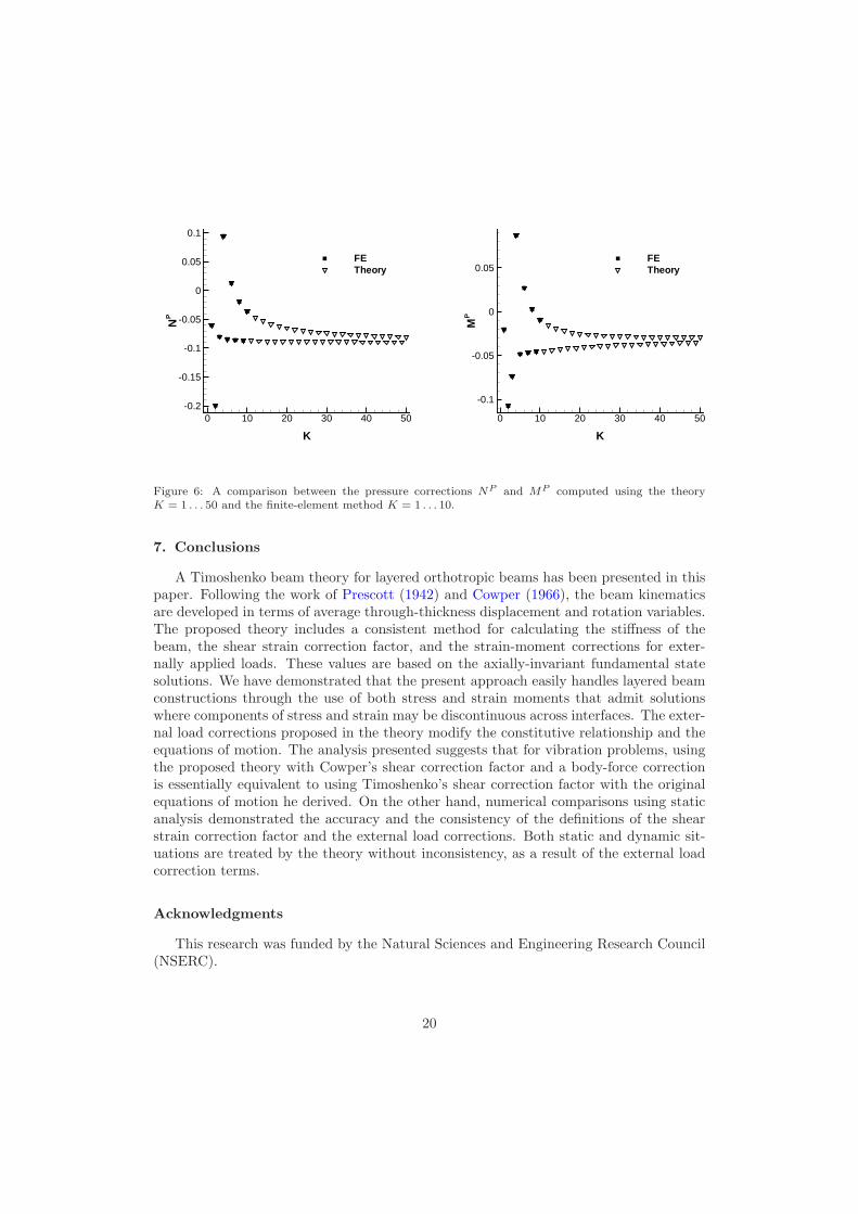
Figure 6 shows the pressure corrections for the axial resultant and bending momentfor the multi-layer beam. The theoretical results were computed by first finding thestrain moment corrections from Equation (18a) and Equation (18b) and multiplying bythe average constitutive relation from Equation (9). The average relative error for thepressure corrections are 3.6 × 10−5 and 4.6 × 10−5 for NP and MP , respectively, whilethe maximum errors are, 1.8× 10−4 and 1.2× 10−4. These results demonstrate that theconstitutive equation is modified by the presence of an externally applied pressure load,otherwise the predicted correction would be zero. In addition, these results show that

17

Core fraction (r)

Sh

ear

corr

ectio

nfa

cto

r(k

xy)

0 0.2 0.4 0.6 0.8 1

0.7

0.75

0.8

0.85

0.9

0.95

1 FEα = 1α = 0.5α = 0.1α = 0.01Limit α = 0

Core fraction (r)

D33

/G

0 0.2 0.4 0.6 0.8 10

0.2

0.4

0.6

0.8

1

FEα = 1α = 0.5α = 0.1α = 0.01

Figure 4: A comparison between the shear correction factor kxy and homogenized shear stiffness D33

computed using the theory and the finite-element method for the three-layer beam.

these corrections are correctly predicted by Equation (18).

6.1. Impact of the corrections

We have demonstrated good agreement between the shear strain correction factor andthe pressure correction when compared with finite-element computations. To put theseresults in perspective, it is necessary to assess the relative importance of these values inpredicting the stress or strain distribution and the deflection of a beam. This is a complextask that is highly problem-dependent. To make a concrete comparison, we examine twocases: the deflection of a tip-loaded cantilever beam and the stress distribution in aclamped-clamped pressure loaded beam.

For the case of the tip-loaded beam, we assess the importance of the shear correctionfactor and homogenized shear stiffness. With no stretching-bending coupling, D12 andD21 are zero and the tip deflection is

v0(L) = Q

[

(

L

2c

)34

D22+

(

L

2c

)

1

D33kxy

]

.

The two terms in this expression represent a contribution to the deflection from thebending stiffness and a contribution from the shear stiffness. The ratio of these two termsis,

rsb =

(

2c

L

)2D22

4D33kxy,

where rsb is the shear to bending displacement ratio. Clearly the slenderness ratio,Sr = L/2c, is the most important single factor. For an isotropic beam, D22 = E andD33 = G, with kxy equal to Cowper’s shear correction factor (2). For a Poisson ratio ofν = 0.3, this results in rsb = 0.765S−2

r . For a reasonable slenderness ratio of Sr > 10,the shear contributes very little to the deflection. On the other hand, for the three-layer

18

K

k xy

0 10 20 30 40 50

0.72

0.74

0.76

0.78

0.8

0.82

0.84

FETheory

K

D33

/G

10 20 30 40

0.158

0.16

0.162

0.164

0.166

0.168

FETheory

Figure 5: A comparison between the shear correction factor kxy and homogenized shear stiffness D33

computed by theory and the finite-element method for the multi-layer beam.

symmetric beam discussed above, with ν = 0.3, α = 0.01, and a core ratio r = 0.95,the shear to bending displacement ratio is rsb = 10.14S−2

r . This suggests that theshear stiffness plays a much more important role in beams of this construction. Correctdetermination of the shear strain correction factor and homogenized shear stiffness ismuch more important for beams that have low shear stiffness such as sandwich beams.

We now examine a clamped-clamped beam subject to a distributed pressure load onthe top and the bottom surfaces, Pt = 4/5 and Pb = 1/5. The beam is composed ofalternating layers as described above for the K = 5 case. The dimensions of the beamare L = 10 and c = 1/2.

The pressure correction causes two effects: a modification of the constitutive relation,and additional contributions to the stress reconstruction (7). Using the constitutiveEquation (9) and the force method, the stress resultants can be determined:

N(x) = −PNP ,

M(x) = P

(

x

2(L− x)−

L2

12−MP

)

,

Q(x) = P

(

L

2− x

)

.

Note that even though the beam is symmetric, there is a non-zero axial compressive forceand moment offset. This is due to the strain moments caused by the pressure on the topand bottom surface of the beam.

Figure 7 shows a comparison of σy and σxy predicted by the stress reconstructionand the finite-element method over the length of beam at a location y = 0.6c. Theseresults show very good agreement between the stress reconstruction and the finite-elementresults. Neglecting the fundamental state corresponding to pressure would result inσy = 0.

19

K

NP

0 10 20 30 40 50-0.2

-0.15

-0.1

-0.05

0

0.05

0.1

FETheory

K

MP

0 10 20 30 40 50

-0.1

-0.05

0

0.05FETheory

Figure 6: A comparison between the pressure corrections NP and MP computed using the theoryK = 1 . . . 50 and the finite-element method K = 1 . . . 10.

7. Conclusions

A Timoshenko beam theory for layered orthotropic beams has been presented in thispaper. Following the work of Prescott (1942) and Cowper (1966), the beam kinematicsare developed in terms of average through-thickness displacement and rotation variables.The proposed theory includes a consistent method for calculating the stiffness of thebeam, the shear strain correction factor, and the strain-moment corrections for exter-nally applied loads. These values are based on the axially-invariant fundamental statesolutions. We have demonstrated that the present approach easily handles layered beamconstructions through the use of both stress and strain moments that admit solutionswhere components of stress and strain may be discontinuous across interfaces. The exter-nal load corrections proposed in the theory modify the constitutive relationship and theequations of motion. The analysis presented suggests that for vibration problems, usingthe proposed theory with Cowper’s shear correction factor and a body-force correctionis essentially equivalent to using Timoshenko’s shear correction factor with the originalequations of motion he derived. On the other hand, numerical comparisons using staticanalysis demonstrated the accuracy and the consistency of the definitions of the shearstrain correction factor and the external load corrections. Both static and dynamic sit-uations are treated by the theory without inconsistency, as a result of the external loadcorrection terms.

Acknowledgments

This research was funded by the Natural Sciences and Engineering Research Council(NSERC).

20

X

σ xy σ y

0 2 4 6 8 10

-4

-2

0

2

4

-2

-1

0

1

2

σy

σxy

σyFE

σxyFE

Figure 7: A slice of the stress distribution at y = 0.6c for a clamped-clamped beam with distributedpressure load on the top and bottom surface, Pt = 4/5 and Pb = 1/5. This location corresponds to aninterface between the top and and next lowest layers.

References

Cowper, G., 1966. The shear coefficient in Timoshenko’s beam theory. Journal of Applied Mechanics33 (5), 335–340.

Dong, S., Alpdogan, C., Taciroglu, E., 2010. Much ado about shear correction factors in Timoshenkobeam theory. International Journal of Solids and Structures 47 (13), 1651 – 1665.URL http://www.sciencedirect.com/science/article/B6VJS-4YH56DC-2/2/21f0dd8f7d8e2e484f97b062d810c136

Flower, H., Soutis, C., 2003. Materials for airframes. The Aeronautical Journal 107 (1072), 331–341.Guiamatsia, I., 2010. A new approach to plate theory based on through-thickness homogenization.

International Journal for Numerical Methods in Engineering.URL http://dx.doi.org/10.1002/nme.2934

Guiamatsia, I., Hansen, J. S., 2004. A homogenization-based laminated plate theory. ASME ConferenceProceedings 2004 (47004), 421–436.URL http://link.aip.org/link/abstract/ASMECP/v2004/i47004/p421/s1

Hansen, J., Kennedy, G. J., de Almeida, S. F. M., 2005. A homogenization-based theory for laminatedand sandwich beams. In: 7th International Conference on Sandwich Structures. Aalborg University,Aalborg, Denmark, pp. 221–230.

Hansen, J. S., Almeida, S. d., April 2001. A theory for laminated composite beams. Tech. rep., InstitutoTecnologico de Aeronautica.

Hutchinson, J. R., 1980. Vibration of solid cylinders. Journal of Applied Mechanics 47 (12), 901–907.Hutchinson, J. R., 1981. Transverse vibration of beams, exact versus approximate solutions. Journal of

Applied Mechanics 48 (12), 923–928.Hutchinson, J. R., 2001. Shear coefficients for Timoshenko beam theory. Journal of Applied Mechanics

68 (1), 87–92.URL http://link.aip.org/link/?AMJ/68/87/1

Kaneko, T., 1975. On Timoshenko’s correction for shear in vibrating beams. Journal of Physics D:Applied Physics 8 (16), 1927–1936.URL http://stacks.iop.org/0022-3727/8/i=16/a=003

Leibowitz, R. C., Kennard, E. H., 1961. Theory of freely-vibrating nonuniform beams, including methodsof solution and application to ships.

Love, A. E. H., 1920. A Treatise on the Mathematical Theory of Elasticity, 3rd Edition. CambridgeUniversity Press.

Pickett, G., 1944. Application of the Fourier method to the solution of certain boundary problems inthe theory of elasticity. Journal of Applied Mechanics 11, 176–182.

21

Prescott, J., 1942. Elastic waves and vibrations of thin rods. Philosophical Magazine 33, 703–754.URL http://www.informaworld.com/10.1080/14786444208521261

Shames, I. H., Dym, C. L., 1985. Energy and Finite Element Methods in Structural Mechanics. McGrawHill Higher Education.

Spence, G. B., Seldin, E. J., 1970. Sonic resonances of a bar and compound torsion oscillator. Journalof Applied Physics 41 (8), 3383–3389.URL http://link.aip.org/link/?JAP/41/3383/1

Stephen, N. G., 1980. Timoshenko’s shear coefficient from a beam subjected to gravity loading. Journalof Applied Mechanics 47 (1), 121–127.URL http://link.aip.org/link/?AMJ/47/121/1

Stephen, N. G., 2001. Discussion: ”Shear coefficients for Timoshenko beam theory”. Journal of AppliedMechanics 68 (11), 959–960.

Stephen, N. G., Levinson, M., 1979. A second order beam theory. Journal of Sound and Vibration 67 (3),293–305.

Tafeuvoukeng, I. G., 2007. A unified theory for laminated plates. Ph.D. thesis, University of Toronto.Timoshenko, S. P., 1921. On the correction for shear of the differential equation for transverse vibrations

of prismatic bars. Philosophical Magazine 41, 744–746.Timoshenko, S. P., 1922. On the transverse vibrations of bars of uniform cross-section. Philosophical

Magazine 43, 125 – 131.

22