A TWO-DIMENSIONAL, FINITE-DIFFERENCE MODEL OF THE PHASE DISTRIBUTION AND VAPOR TRANSPORT OF MULTIPLE COMPOUNDS A Thesis Presented to the Faculty of San Diego State University In Partial Fulfillment of the Requirements for the Degree Master of Science in Geology by David A. Benson Spring 1992
Transcript
A TWO-DIMENSIONAL, FINITE-DIFFERENCE MODEL
OF THE PHASE DISTRIBUTION AND VAPOR
TRANSPORT OF MULTIPLE COMPOUNDS
A Thesis
Presented to the
Faculty of
San Diego State University
In Partial Fulfillment
of the Requirements for the Degree
Master of Science
in
Geology
by
David A. Benson
Spring 1992
iii
Copyright
December 23, 1991
by David A. Benson
iv
ACKNOWLEDGEMENTS
I would like to thank my wife Marnee for knowing what 6 x 7 was when I really
needed it (and for the higher math). Also, many thanks to Paul Johnson for help in
verification, Donn Marrin for being an actual certifiable professor, adjunct though he
is, and Dave Huntley for meaning it when he says he’ll get right to it - in a couple of
months. I also owe a great deal to Melissa Matson, because she couldn’t have been
paid enough to track down my stuff.
v
TABLE OF CONTENTS
PAGE
ACKNOWLEDGEMENTS ......................................................................................... iv
LIST OF FIGURES.....................................................................................................vii
CHAPTER
I. INTRODUCTION................................................................................................ 1
II. THEORETICAL BACKGROUND ..................................................................... 4
General Transport Equation ........................................................................ 4
Calculation of Flow Regime ....................................................................... 8
FIGURE PAGE1. Schematic representation of model structure. .............................................. 26
2. Elimination of negative concentrations by using a "donor-cell" calculation of soil gas movement. .................................... 30
3. Comparison of venting simulations using Johnsonet al. (1990) model (solid lines) and the presentwork in a non-transport mode (symbols). .............................................. 37
4. Comparison of modeled pressure distributionand the radial analytic solution............................................................... 39
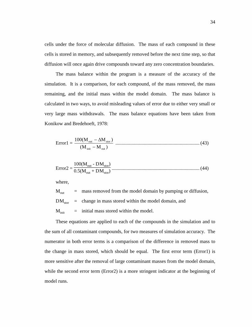
5. One-dimensional transport of retarded compounds. .................................... 41
6. Comparison of remediation time for different plume geometry. ................. 43
7. Comparison of residual gasoline mass during ventingof homogeneous versus layered permeability models. ........................... 46
8. Residual "hot-spot" maximum observed gasolineconcentrations during venting of homogeneousversus layered permeability model ......................................................... 48
9. Comparison of benzene flux using single componentor gasoline mixture formulation............................................................. 49
10. Simulated gasoline distribution after 200 days ofventing from a single well: a) with surfaceleakage; and, b) without surface leakage................................................ 50
1
CHAPTER I
INTRODUCTION
It has been estimated by the United States Environmental Protection Agency
that as much as 30 percent of the 3.5 million underground storage tanks containing
petroleum hydrocarbons and other potentially hazardous materials are leaking (Dowd,
1984). A large portion of these leaking tanks have introduced petroleum fuels and
other mixtures of volatile organic liquids into the environment. Once placed into the
unsaturated zone, the fluids will move in response to gravity and soil tension, leaving
behind significant quantities of immiscible, non-aqueous phase liquid (NAPL) held
stably in place by capillary forces (an excellent overview is given by Hunt, et al.,
1988). If a large enough quantity is released, the immiscible liquid will reach the
water table, and, depending on the contaminant density, either accumulate in a
floating layer or continue to travel downward through the saturated zone. Depending
on the physical qualities of the contaminant mixture, a significant portion will
volatilize and migrate through the unsaturated zone at much higher rates than the
liquid phases.
The main threat to human health resulting from subsurface toxic compound
releases has long been recognized as the movement of dissolved components in
groundwater toward production wells. To address this threat, the thrust of remedial
measures has been dominated by the extraction and treatment of large quantities of
2
groundwater. The observation of many protracted "pump-and-treat" methodologies
has prompted more aggressive treatment of the contaminant sources, which may or
may not be located within the saturated zone. In the case of lighter-than-water
nonaqueous phase liquids (LNAPLs), product recovery methods include liquid
extraction with or without attempted enhancement by water table depression (Nyer,
1985) and, more recently, vacuum-enhanced skimming (Blake, et al., 1990).
The need to address the residual contaminants that remain in the unsaturated
zone, either above the original water table or an artificially depressed phreatic surface,
has resulted in the profusion of vapor extraction as a remediation technique. By
inducing the flow of soil vapor through volumes of soil containing the volatile
compounds, levels of residual contamination can be significantly reduced. Vapor
extraction is a particularly attractive remedial alternative because of the relative low
cost, the virtual non-interruption of normal activities at commercial and industrial
sites, and the ability to clean deeply buried soil.
Several factors are directly related to the rate at which contaminants can be
removed from soil, and should be simulated in the assessment of vapor extraction
feasibility or remedial system design. These factors include the distribution of soil
permeability (and resultant flow fields), the distribution and composition of the
contaminant mixture, soil properties which effect the vapor concentrations of the
chemical compounds, and the placement of vapor extraction or injection wells. A
number of vapor transport models have been formulated based on the occurrence of
one compound that is present in three phases (no NAPL). This simplification allows
the models to assign a constant value of retardation to the compound (Jury, et al.,
1983; Mendoza and Frind, 1990; Sleep and Sykes, 1989; Falta et al. 1989).
3
Non-dimensional chemical equilibrium models were developed by Marley and
Hoag (1984) and Johnson, et al., (1990) to describe the concentrations of compounds
in vapor above a liquid chemical mixture of known composition, and to predict the
changes in those concentrations with subsequent removals of quantities of vapor.
These models neglect variability in the vapor-flow fields and contaminant
distribution, but were certainly more representative of sites requiring remediation,
because they included a fourth (NAPL) phase. Baehr and Hoag (1988) demonstrated
a one-dimensional simulation of column experiments which included a four-phase
chemical equilibrium formulation, but assumed zero retardation and a constant value
for vapor discharge.
In this paper, a model is presented which mathematically simulates the
advective and diffusive transport of virtually any number chemical compounds
simultaneously in two dimensions. The model also explicitly solves the distribution
of each compound among four phases (vapor, adsorbed, dissolved, and NAPL),
thereby simulating the differing retarded movement of compounds with variable
properties. The model tracks contaminant saturation and recalculates the flow regime
to reflect the depletion of pore fluids.
4
CHAPTER II
THEORETICAL BACKGROUND
General Transport Equation
Consider a volume of soil contaminated with any number of chemical
compounds. If the soil is within the vadose zone, then a portion of the contaminant
will be present in the soil gas. Each of the compounds will be distributed within four
phases: a vapor phase, a dissolved soil moisture phase, an adsorbed phase, and, if total
soil concentrations are high enough, a separate non-aqueous phase (Marley and Hoag,
1984; Johnson, et al., 1990). The purpose of the model contained herein is to describe
the movement of compounds in the vapor phase, and the phase distribution of each
compound. The movement of the gaseous compounds may be due to molecular
diffusion, the advective motion of carrier soil gas, or a combination of both.
If a volume of partially evacuated (vadose zone) soil is represented by the
differential volume dxdydz, then the net chemical vapor flux in each axial direction is
A computer program has been generated to fill a gap in the tools used for
remedial simulation. Just as non-ideal groundwater aquifer conditions warrant the use
of higher-order solute transport models, similar conditions in the unsaturated zone
indicate the same treatment with vapor transport simulation. Some additional
parameters in the unsaturated zone, including a variable number of phases and
continually changing pneumatic conductivity, make such simulations somewhat more
complex. However, with diffusion coefficients of most vapors being so much higher
than water diffusion coefficients, dispersion can be handled without velocity
dependance. This simplification enables creating a program that can be easily used on
a 32-bit personal computer. For example, a 400 node, 50 chemical compound version
of the code compiles in less than 300 kilobytes. Further, the addition of a third
dimension poses no real computational difficulties, if more representative free-
product layer simulation is desired. A side benefit of the model happens to be the
ability to more accurately track the natural diffusion of compounds in fate and
transport simulation for risk assessment.
The utility of the model has been demonstrated by simulating several
hypothetical vapor extraction remediation scenarios. In each of the highly simplified
examples, previous models were unconservative in their estimation of time needed to
reach cleanup by up to 100 percent. Virtually any deviation from a symmetrical
contaminant spill within soil of homogeneous permeability will produce longer
52
remediation time. A number of deviations can be imagined that were not investigated
in this paper, such as the effect of multiple wells producing "dead-spots" of little or no
advective vapor flow. In such a simulation it can be seen and whether diffusion from
these zones will offset that single drawback of adding more wells, or if air-injection
wells are needed.
53
REFERENCES
54
REFERENCES
Baehr, A. L., Hoag, G. E., A modeling and experimental investigation of induced
venting of gasoline-contaminated soils, in Soils contaminated by petroleum,
Calabrese, E. J. and Kostecki, P. T., eds., John Wiley and Sons, 113-123, 1988.
Baehr, A. L., Hoag, G. E., and Marley, M. C., Removing volatile contaminants from
the unsaturated zone by inducing advective air-phase transport; Journal of
Contaminant Hydrology, 4, 1-26, 1989.
Bear, J., Dynamics of Fluids in Porous Media, American Elsevier, 1972.
Blake, S., Martin, M., and Hockman, B., Applications of vacuum dewatering
techniques to hydrocarbon remediation; NWWA/API Conference on Petroleum
Hydrocarbons and Organic Chemicals in Ground Water, Prevention, Detection,
and Restoration, Houston, Texas, October 31-November 2, 1990.
Brooks, R. H., and Corey, A. T., Hydraulic properties of porous media, Hydrol. Pap.
3, 27 pp., Colorado State University, Fort Collins, 1964.
Dowd, R. M., Leaking underground storage tanks, Environ, Sci. Technol. 18(10),
1984.
Falta, R. W., Javendel, I., Pruess, K., and Witherspoon, P. A., Density-driven flow of
gas in the unsaturated zone due to the evaporation of volatile organic
compounds, Water Resources Research, 25(10), 2159-2169, 1989.
Garder, A. O., Peaceman D. W., and Pozzi, A. L., Jr., Numerical calculation of
multidimensional miscible displacement by the method of characteristics,
Society of Petroleum Engineers Journal, 4(1), 26-36, 1964.
55
Goode, D. J., and Konikow, L. F., Modification of a method-of-characteristics solute-
transport model to incorperate decay and equilibrium-controlled sorption or ion
exchange, United States Geological Survey Water-Resources Investigations
report 89-4030, 65 p, 1989.
Hubbert, M. K., The theory of groundwater motion, Journal of Geology 48(8), 1940.
Hunt, J. R., Sitar, N., and Udell, K. S., Nonaqueous phase liquid transport and
cleanup 1. Analysis of mechanisms, Water Resources Research, 24(8), 1247-
1258, 1988.
Johnson, P. C., Kemblowski, M. W., Colthart, J. D., Byers, D. L., and Stanley, C. C.,
A practical approach to the design, operation, and monitoring of in-situ venting
systems, presented at the U.S.E.P.A workshop on vacuum extraction, Edison,
New Jersey, June 28, 29 1989.
Johnson, P. C., Stanley, C. C., Byers, D. L., Benson, D. A., and Acton, M. A., 1989,
Soil venting at a California site: Field data reconciled with theory; First Annual
West Coast Conference, Hydrocarbon Contaminated Soils and Groundwater,
Newport, California, February 22, 1990.
Johnson, P. C., Kemblowski, M. W., and Colthart, J. D., Quantitative analysis for the
cleanup of hydrocarbon-contaminated soils by in-situ soil venting, Ground
Water vol. 28, no. 3, pp. 413-429, 1990.
Jury, W. A., Spencer, W. F., and Farmer, W. J., Behavior assessment model for trace
organics in soil: I. Model description, Journal of Environmental Quality 12(4),
558-564, 1983.
Jury, W. A., Russo, D., Streile, G., and Hesham, E. A., Evaluation of volatilization by
organic chemicals residing below the soil surface, Water Resources Research
26(1) 13-20, 1990.
56
Karickhoff, S. W., Semi-empirical estimation of sorption of hydrophobic pollutants
on natural sediments and soils, Chemosphere, 10(8), 833-846, 1981.
Konikow, L. F., and Bredehoeft, T. D., Computer model of two-dimensional solute
transport and dispersion in ground water, Techniques of Water-Resources
Investigations of the United States Geological Survey, Book 7, Chapter C2, 90
p, 1978.
Marley, M. C., and Hoag, G. E., Induced soil venting for the recovery/restoration of
gasoline hydrocarbons in the vadose zone; NWWA/API Conference on
Petroleum Hydrocarbons and Organic Chemicals in Ground Water, Houston,
Texas, November 5-7, 1984.
Mendoza, C. A., Hughes, B. M., and Frind, E. O., Transport of trichloroethylene
vapours in the unsaturated zone: numerical analysis of a field experiment;
Proceedings, IAH Conference on Subsurface Contamination by Immiscible
Fluids, Calgary, April 18-20, 1990.
Mendoza, C. A., and Frind, E. O., Advective-dispersive transport of dense organic
vapors in the unsaturated zone 1. Model development, Water Resources
Research 26(3) 379-387, 1990.
Millington, R. J., and Quirk, J. P., Permeability of porous solids, Trans. Faraday
Society., 57, 1200-1207, 1961.
Nyer, E. K., Groundwater Treatment Technology, Van Nostrand Reinhold, New
York, 1985.
Parker, J. C., Lenhard, R. J., and Kuppusamy, T., A parametric model for constitutive
properties governing multiphase flow in porous media, Water Resources
Research, 23(4), 618-624, 1987.
57
Prickett, T. A., Naymik, T. G., and Lonnquist, C. G., A random-walk solute transport
for selected groundwater quality evaluations, Bull. Illinois State Water Survey,
65, Champaign, 1981.
Reynolds, W. D., Gillham, R. W., and Cherry, J. A., Evaluation of distribution
coefficients for the prediction of strontium and cesium migration in a uniform
sand; Can. Geotech. Jour., 19(1), 92-103, 1982.
Sleep, B. E., and Sykes, J. F., Modeling the transport of volatile organics in variably
saturated media, Water Resources Research, 25(1), 81-92, 1989.
58
APPENDICES
59
APPENDIX A
FORTRAN PROGRAM LISTING
60
FORTRAN PROGRAM LISTING
Copyright 1991, by David A. BensonAll Rights ReservedTranscription Prohibited
CCCCCCCCCCCCCCCCCCCCCCCCCCCCCCCCCCCCCCCCCCCCCCCCCCCCCCCCCCCCCCCCCCCCCCCCC CC P R O G R A M V E N T 2-D CC CC DAVID A. BENSON 02/28/91 CC CC THIS PROGRAM IS DESIGNED TO SOLVE THE 2-D VAPOR PHASE CC ADVECTIVE AND DIFFUSIVE FLUX OF MIXTURES OF COMPOUNDS. CC IN DOING SO, THE FLOW FIELD IS SOLVED FOR A 20 BY 20 CC ORTHOGONAL GRID. WITHIN THE GRID, ANY NUMBER OF VAPOR CC EXTRACTION AND INJECTION WELLS CAN BE SIMULATED, AND CC GRID-VARIABLE INITIAL PERMEABILITY AND CONTAMINANT DIST- CC RIBUTION IS SIMULATED. THE EQUILIBRIUM 4-PHASE OCCURRENCE CC OF EACH COMPOUND IN THE MIXTURE IS SOLVED BETWEEN CC VAPOR PHASE MOVING PERIODS. THE COMPOUNDS ARE MOVED CC USING A FORWARD EXPLICIT SOLUTION. THE MOVEMENT CC OF SOIL MOISTURE IS SIMULATED, AND PERMEABILITY IS TIME- CC AND-GRID-VARIABLE AS A FUNCTION OF FLUID SATURATION. CC CCCCCCCCCCCCCCCCCCCCCCCCCCCCCCCCCCCCCCCCCCCCCCCCCCCCCCCCCCCCCCCCCCCCCCCCCCC MAKE NC THE NUMBER OF COMPOUNDS + 1 (THE EXTRA IS FOR WATER)C PARAMETER (NC=50)C CHARACTER*30 LCNAME(NC),LTITLE*80,NUL*1,ESC*1 REAL MC(20,20,NC),MCHC(20,20),MCWAT(20,20),MASSF(NC),MW(NC), 1 KD(NC),INTRK(20,20),B,DELT,RUNTIME,TMULT,MOIST COMMON NX,NY,DX,DY,THCK,POR,MOIST,NCOMP,SDENS,DELH2O,RUNTIME, 1 DELT,TMULT,TEMP,QX(20,20),QY(20,20),VOID(20,20),P(20,20), 2 PERM(20,20),PERMX(20,20),PERMY(20,20),MC,CI(20,20,NC), 3 PUMPMOLE(NC),W(20,20),C(20,20),MCWAT,TOTMOLE(NC),INTRK, 4 TOTMASS,NSTEPS,IFLAGIMP,ICOMPFL(NC),CELLDIS,WELLCRIT, 5 VPERM(20,20),NWELLS,NZEROC,ZEROC(20,20),DIFFLOSS(NC), 6 FLUXMASS(NC),DENSLIQ,DIFFMAX,DIFFMAXJ COMMON /STRINGS/LCNAME,LTITLE COMMON /VELO/VISC,OMEGA,CRIT,QXMAX,QYMAX COMMON /EQ/MASSF,MW,KD,MCHC,VPWAT,BP(NC),ACT(NC),SOL(NC),VP(NC), 1 FOC,NPHASE(20,20),RETARD(NC) COMMON /MOVE/RH,RHINJ,CINJ,AIRDIFF COMMON /OUT/IFLAGM,IFLAGC,NGRAPH,GRAPH(50,10)CCCCCCCCCCCCCCCCCCCCCCCCCCCCCCCCCCCCCCCCCCC THINGS TO DO IN THE MAIN PROGRAM:C DO THE TIME LOOP, KEEP TRACK OF OUTPUT NEEDS,
61
C FIGURE MOISTURE CONTENT BEFORE PASSING TO EQ.C KEEP TRACK OF CHANGING k/VISC, AND DO MASS BALANCECC BUT FIRST, INPUT THE DATA FILE AND LOAD THE NECESSARY PARAMETERSC CALL GETINC TIME=0.0 NTSTEPS=0 FTIME=0.0 FDELT=DELT NFSTEPS=0 NUL=CHAR(0) ESC=CHAR(27) FTIME=FTIME+DELT 777 CALL FLOW(TIME) NFLOWS=0 888 WRITE(6,400)NUL,ESC WRITE(6,*)NFSTEPS,’ STEPS HAVE BEEN COMPLETED OF ’, NSTEPS TMOLE=0.0 DO 10 I=1,NX DO 10 J=1,NY C(I,J)=0.0 DO 11 N=1,NCOMP C(I,J)=C(I,J)+(MC(I,J,N)*MW(N)*1.0E06)/SDENS TMOLE=TMOLE+MC(I,J,N) 11 CONTINUE IF(C(I,J).GT.0.0) THEN VOID(I,J)=POR-(C(I,J)*SDENS/(1.0E06*DENSLIQ))- 1 MC(I,J,NCOMP+1)*18.0 ELSE VOID(I,J)=POR-MC(I,J,NCOMP+1)*18.0 ENDIF EVAC=VOID(I,J)CCCCCCCCCCCCCCCCCCCCCCCCCCCCCCCCCCCC CALL THE SUBROUTINE TO ITERATE THE CHEMICAL EQUILIBRIUMC AT THIS NODE CALL EQUIL(I,J,EVAC,NTSTEPS) 10 CONTINUECCCCCCCCCCCCCCCCCCCCCCCCCCCCCCCCCCCC CALCULATE TOTAL VAPOR MOLES AT EACH NODE FOR USEC IN THE DETERMINATION OF ACTUAL TIME STEP SIZEC DO 13 I=1,NX DO 13 J=1,NY GMOLE=0.0 IF(W(I,J).LT.0.0) THEN DO 14 N=1,NCOMP GMOLE=GMOLE+CI(I,J,N) 14 CONTINUE DT1=-1.0*WELLCRIT*TMOLE*DX*DY*THCK/(GMOLE*W(I,J)) IF((DT1.GT.0.0).AND.(DT1.LT.DELT)) THEN DELT=DT1 WRITE(6,340)DELT/(60.0*1440.0),TIME/(60.0*1440.0) WRITE(6,401)NUL,ESC ENDIF ENDIF
62
13 CONTINUECC----------DETERMINE TIME STEP SIZE FOR EXPLICIT SOLUTIONC AND SET UP ANSI.SYS ROUTINEC if((nwells).gt.0) then DTTEMP=CELLDIS*evac*(MIN((DX/QXMAX),(DY/QYMAX))) IF(DTTEMP.LT.DELT) THEN DELT=DTTEMP WRITE(6,350)DELT/(60.0*1440.0),TIME/(60.0*1440.0) WRITE(6,401)NUL,ESC ENDIF endif if(airdiff.gt.0.0) then dttemp=0.5/((airdiff/dx**2.0)+(airdiff/dy**2.0)) if(ntsteps.gt.0) DTTEMP=0.45/DIFFMAX IF(DTTEMP.LT.DELT) THEN DELT=DTTEMP WRITE(6,370)DELT/(60.0*1440.0),TIME/(60.0*1440.0) WRITE(6,401)NUL,ESC ENDIF endif IF((TIME+DELT).GT.FTIME) THEN DELT=FTIME-TIME FDELT=FDELT*TMULT FTIME=FTIME+FDELT NFSTEPS=NFSTEPS+1 WRITE(6,360)DELT/(60.0*1440.0),TIME/(60.0*1440.0) WRITE(6,401)NUL,ESC CALL OUTPUT(NFLOWS,NFSTEPS,TIME) elseif(time.eq.0.0) then WRITE(6,360)DELT/(60.0*1440.0),TIME/(60.0*1440.0) WRITE(6,401)NUL,ESC CALL OUTPUT(NFLOWS,NFSTEPS,TIME) ENDIFCCCCCCCCCCCCCCCCCCCCCCCCCCCCCCCCCCCCCCCC CALL THE DESIRED SUBROUTINE TO MOVE THE COMPOUNDS AND WATERC IF(IFLAGIMP.LT.1) THEN CALL MOVEIMP(NFLOWS) ELSE CALL MOVEEXP(NFLOWS) ENDIFCCCCCCCCCCCCCCCCCCCCCCCCCCCCCCCC INCREMENT THE TIME COUNTER AND RESET DELTA TIMEC TIME=TIME+DELT DELT=FDELTCCCCCCCCCCCCCCCCCCCCCCCCCCCCCCCCCCCCCCC RECALCULATE THE RELATIVE GAS PERMEABILITY, AND IF 10 PERCENTC OF THE CELLS HAVE CHANGED 25% OR MORE, RECALCULATE THE FLOWC PARAMETERS.CC IF(TIME.LT.RUNTIME) THEN
63
NFLOWS=NFLOWS+1 NTSTEPS=NTSTEPS+1 DO 25 I=1,NX DO 25 J=1,NY SATGAS=VOID(I,J)/POR PERMNEW=INTRK(I,J)*SATGAS**3.0 IF (ABS(PERMNEW-PERM(I,J))/PERM(I,J).GT.0.25) THEN NRECALC=NRECALC+1 ENDIF PERM(I,J)=PERMNEW 25 CONTINUE IF(NRECALC.GT.(NX*NY/10)) GO TO 777 GO TO 888 ELSE CALL OUTPUT(NFLOWS,NFSTEPS,TIME) STOP ENDIFCCCCCCCCCCCCCCCCCCCCCCCCCCCCCC FORMATSC 300 FORMAT(’ MOLE BALANCE CALCUALATIONS AT TIME = ’, F7.2,’ DAYS’ 1 /’ COMPOUND # PERCENT ERROR’) 310 FORMAT(1X,I5,14X,F7.2) 320 FORMAT(’ MASS BALANCE CALCUALATIONS AT TIME = ’, F7.2,’ DAYS’/ 1 ’ NET PUMPED MASS MASS REMAINING INITIAL MASS MASS’, 2 ’ ERROR (%)’,’ ERROR (%)’) 330 FORMAT(1X,G10.4,6X,G10.4,10X,G10.4,6X,G10.4,6X,G10.4) 340 FORMAT(1X,’TIME STEP SIZE = ’,G10.4,’ AT TIME:’, 1 G10.4,’ DAYS, DUE TO PUMP TERM’) 350 FORMAT(1X,’TIME STEP SIZE = ’,G10.4,’ AT TIME:’, 1 G10.4,’ DAYS, DUE TO MAX VELOCITY’) 360 FORMAT(1X,’TIME STEP SIZE = ’,G10.4,’ AT TIME:’, 1 G10.4,’ DAYS, TO ADJUST TO PRINTOUT TIME’) 370 FORMAT(1X,’TIME STEP SIZE = ’,G10.4,’ AT TIME:’, 1 G10.4,’ DAYS, DUE TO DIFFUSION TERM’)CC---------THIS FORMAT STATEMENT REQUIRES ANSI.SYSC 400 FORMAT(2A1,’[2A’) 401 FORMAT(2A1,’[2A’) ENDCCCCCCCCCCCCCCCCCCCCCCCCCCCCCCCCCCCCCCCCCCCCCCCCCCCCCCCCCCCCCCCCCCCCCCCCCC S U B R O U T I N E G E T I N CCCCCCCCCCCCCCCCCCCCCCCCCCCCCCCCCCCCCCCCCCCCCCCCCCCCCCCCCCCCCCCCCCCCCCCCCC CC THIS SUBROUTINE READS IN ALL OF THE GRID, SOIL, AND CHEMICAL CC PARAMETERS. VALUES WHICH DO NOT CHANGE DURING THE SIMULATION CC (ACTIVITIES, PURE COMPONENT VAPOR PRESSURES, ETC.) ARE CC INITIALIZED HERE. CC CCCCCCCCCCCCCCCCCCCCCCCCCCCCCCCCCCCCCCCCCCCCCCCCCCCCCCCCCCCCCCCCCCCCCCCCC SUBROUTINE GETIN PARAMETER (NC=50) CHARACTER*40 FILEIN,FILEOUT,FILEGR CHARACTER*30 LCNAME(NC),LTITLE*80 REAL MC(20,20,NC),MCHC(20,20),MCWAT(20,20),MASSF(NC),MW(NC), 1 KD(NC),INTRK(20,20),B,DELT,RUNTIME,TMULT,MOIST COMMON NX,NY,DX,DY,THCK,POR,MOIST,NCOMP,SDENS,DELH2O,RUNTIME,
64
1 DELT,TMULT,TEMP,QX(20,20),QY(20,20),VOID(20,20),P(20,20), 2 PERM(20,20),PERMX(20,20),PERMY(20,20),MC,CI(20,20,NC), 3 PUMPMOLE(NC),W(20,20),C(20,20),MCWAT,TOTMOLE(NC),INTRK, 4 TOTMASS,NSTEPS,IFLAGIMP,ICOMPFL(NC),CELLDIS,WELLCRIT, 5 VPERM(20,20),NWELLS,NZEROC,ZEROC(20,20),DIFFLOSS(NC), 6 FLUXMASS(NC),DENSLIQ COMMON /STRINGS/LCNAME,LTITLE COMMON /VELO/VISC,OMEGA,CRIT,QXMAX,QYMAX COMMON /EQ/MASSF,MW,KD,MCHC,VPWAT,BP(NC),ACT(NC),SOL(NC),VP(NC), 1 FOC,NPHASE(20,20),RETARD(NC) COMMON /MOVE/RH,RHINJ,CINJ,AIRDIFF COMMON /OUT/IFLAGM,IFLAGCCCCCCCCCCCCCCCCCCCCCCCCCCCCCCCCCCCCCCCCCCCCC FIND OUT THE INPUT AND OUTPUT FILENAMES AND READ DATAC WRITE(6,*)’ENTER THE INPUT FILENAME: ’ READ(5,10)FILEIN WRITE(6,*)’ENTER THE OUTPUT FILENAME: ’ READ(5,10)FILEOUT WRITE(6,*)’ENTER TIME V. CONC. OUTPUT FILENAME: ’ READ(5,10)FILEGR 10 FORMAT(A40) OPEN(UNIT=9,FILE=FILEIN,STATUS=’OLD’) OPEN(UNIT=8,FILE=FILEOUT,STATUS=’UNKNOWN’) OPEN(UNIT=10,FILE=FILEGR,STATUS=’UNKNOWN’) READ(9,11)LTITLE 11 FORMAT(A80) READ(9,*)NX,DX,NY,DY,THCK,POR,MOIST,NWELLS,NZEROC READ(9,*)SDENS,TEMP,OMEGA,CRIT,RH,RHINJ,CINJ READ(9,*)NCOMP,DENSLIQ,AIRDIFF,FOC READ(9,*)RUNTIME,NSTEPS,TMULT,CELLDIS,WELLCRIT READ(9,*)IFLAGM,IFLAGC,IFLAGIMP DO 15 I=1,NX DO 15 J=1,NY W(I,J)=0.0 P(I,J)=1.013E6**2.0 ZEROC(I,J)=-999.9 15 CONTINUECCCCCCCCCCCCCCCCCCCCCCCCCCCCCCCCCCC READ IN THE WELL LOCATIONS AND FLOWRATES (EXTRACT=NEGATIVE)C CONVERT L/MIN TO CC/SECC IF(NWELLS.GT.0) THEN DO 20 N=1,NWELLS READ(9,*)I,J,W(I,J) WRITE(6,*)’WELL AT NODE’,I,’,’,J,’FLOWRATE:’,W(I,J),’ L/MIN’ W(I,J)=W(I,J)*1000.0/60.0 20 CONTINUE ENDIFCCCCCCCCCCCCCCCCCCCCCCCCCCCCCCCCCCCC READ IN THE LOCATION OF CONSTANT CONCENTRATION NODESC FOR USE IN DIFFUSION ONLY SIMULATIONSC IF(NZEROC.GT.0) THEN DO 30 N=1,NZEROC
65
READ(9,*)I,J ZEROC(I,J)=0.0E-33 30 CONTINUE ENDIFCCCCCCCCCCCCCCCCCCCCCCCCCCCCCCCCCCCC READ IN AQUIFER INTRINSIC PERMEABILITIES IN DARCIESC CONVERT TO k/VISC IN CM**3*S/GMC VISC=1.8E-04 READ(9,*)INFLAG,FACTOR DO 40 J=NY,1,-1 IF(INFLAG.EQ.1) READ(9,*)(INTRK(I,J),I=1,NX) DO 40 I=1,NX IF(INFLAG.NE.1) THEN INTRK(I,J)=(FACTOR*1.0E-08)/VISC ELSE INTRK(I,J)=(INTRK(I,J)*FACTOR*1.0E-08)/VISC ENDIF 40 CONTINUECCCCCCCCCCCCCCCCCCCCCCCCCCCCCCCCCCCCCCCCCCCCCCCCCCCCCCCCCCCC READ IN THE VERTICAL LEAKANCE ARRAY IN, YES, DARCY/FEETC AND CONVERT TO CM**2*S/GMC READ(9,*)INFLAG,FACTOR,OVERBRDN DO 50 J=NY,1,-1 IF(INFLAG.EQ.1) READ(9,*)(VPERM(I,J),I=1,NX) DO 50 I=1,NX IF(INFLAG.NE.1) THEN VPERM(I,J)=(FACTOR*1.0E-08)/(VISC*(OVERBRDN*12.0*2.54)) ELSE VPERM(I,J)=(VPERM(I,J)*FACTOR*1.0E-08)/ 1 (VISC*(OVERBRDN*12.0*2.54)) ENDIF 50 CONTINUECCCCCCCCCCCCCCCCCCCCCCCCCCCCCCCCCCCCCCCCC READ IN THE INITIAL CONCENTRATION ARRAY IN MG/KG UNITSC READ(9,*)INFLAG,FACTOR DO 60 J=NY,1,-1 IF(INFLAG.EQ.1) READ(9,*)(C(I,J),I=1,NX) DO 60 I=1,NX IF(INFLAG.NE.1) THEN C(I,J)=FACTOR ELSE C(I,J)=C(I,J)*FACTOR ENDIF TOTMASS=TOTMASS+C(I,J) 60 CONTINUE TOTMASS=TOTMASS*DX*DY*THCK*SDENS*1.0E-6 WRITE(6,*)’TESTING 1 - TOTAL MASS (GRAMS) = ’,TOTMASSCCCCCCCCCCCCCCCCCCCCCCCCCCCCCCCCCCCCCCCCCCCC READ IN THE COMPOUND PARAMETERSC
66
NGRAPH=0 DO 70 I=1,NCOMP write(6,*)I,NCOMP,MASSF(I),MW(I),BP(I),VP(I),SOL(I),KD(I), 1 ICOMPFL(I) READ(9,*)MASSF(I),MW(I),BP(I),VP(I),SOL(I),KD(I), 1 ICOMPFL(I) write(6,*)I,NCOMP,MASSF(I),MW(I),BP(I),VP(I),SOL(I),KD(I), 1 ICOMPFL(I) NGRAPH=NGRAPH+ICOMPFL(I) 70 CONTINUE DO 71 N=1,NCOMP READ(9,110)LCNAME(N) 71 CONTINUE MW(NCOMP+1)=18.0 LCNAME(NCOMP+1)=’WATER’ ICOMPFL(NCOMP+1)=1 110 FORMAT(A30)CCCCCCCCCCCCCCCCCCCCCCCCCCCCCCCCCCCCCCCCCCCCC CALCULATE NEEDED PARAMETERS OF VAPOR PRESSURE AT TEMP,C PARTITIONING COEFFICIENT, AND ACTIVITY COEFFICIENTSC TEMP=TEMP+273.0 REF=293.0 DO 80 I=1,NCOMP BPK=BP(I)+273.0 VP(I)=VP(I)*EXP((BPK*REF/(BPK-REF))*(1.0/TEMP-1.0/REF)* 1 LOG(VP(I))) ACT(I)=55.55*MW(I)/(SOL(I)/1000.0) IF(VP(I).GE.1.0) ACT(I)=ACT(I)/VP(I) KD(I)=0.63*KD(I)*FOC 80 CONTINUE VPWAT=0.023*EXP((373.*293./(373.-293.))*(1./TEMP-1./293.)* 1 LOG(0.023))CCCCCCCCCCCCCCCCCCCCCCCCCCCCCCCCCCCCCCCC CONVERT MASS FRACTIONS TO MOLE FRACTIONSC AND PLACE THIS COMPOSITION INTO EACH GRID CELL.C EACH CELL CARRIES THE MOLES OF EACH COMPOUND PER VOLUME SOIL.C TOTMASS=0.0 DO 95 N=1,NCOMP TOTMOLE(N)=0.0 DO 96 I=1,NX DO 96 J=1,NY MC(I,J,N)=(C(I,J)*SDENS/1.0E06)*MASSF(N)/MW(N) TOTMOLE(N)=TOTMOLE(N)+MC(I,J,N)*THCK*DX*DY IF((ZEROC(I,J).GT.-1.0).AND.(C(I,J).GT.0.0)) THEN WRITE(6,*)’BIG PROBLEM: POSITIVE CONCENTRATIONS SPECIFIED 1 IN ZERO CONC. NODE!’ ENDIF 96 CONTINUE TOTMASS=TOTMASS+(TOTMOLE(N)*MW(N)) 95 CONTINUE WRITE(6,*)’TESTING - TOTAL CONTAMINANT MASS:’,TOTMASS,’ GRAMS’CCCCCCCCCCCCCCCCCCCCCCCCCCCCCCCCCCCCCCCCC NOW FIGURE THE IMPORTANT INITIAL VALUES OF EACH CELL
67
C TOTMOLE(NCOMP+1)=0.0 TEMPSAT=POR-SDENS*MOIST DO 97 I=1,NX DO 98 J=1,NY IF((I.EQ.1).OR.(I.EQ.NX).OR.(J.EQ.1).OR.(J.EQ.NY)) THEN MC(I,J,NCOMP+1)=0.0 ELSE MC(I,J,NCOMP+1)=SDENS*MOIST/18.0 ENDIF VOID(I,J)=POR-(C(I,J)*SDENS/(1.0E06*DENSLIQ))- 1 MC(I,J,NCOMP+1)*18.0 SATGAS=VOID(I,J)/POR PERM(I,J)=INTRK(I,J)*SATGAS**3.0 VPERM(I,J)=VPERM(I,J)*TEMPSAT**3.0 TOTMOLE(NCOMP+1)=TOTMOLE(NCOMP+1)+MC(I,J,NCOMP+1)*DX*DY*THCK 98 CONTINUE 97 CONTINUECCCCCCCCCCCCCCCCCCCCCCCCCCCCCCCCCCCCCCCCCCCC FIGURE SOME OF THE RUN PARAMETERS - DELT IS IN SECONDS,C WHILE RUNTIME IS INPUT IN DAYSC SUMTEMP=1.0 SUMTEMP2=1.0 DO 99 M=1,NSTEPS-1 SUMTEMP2=SUMTEMP2*TMULT SUMTEMP=SUMTEMP+SUMTEMP2 99 CONTINUE DELT=RUNTIME*1440.0*60.0/SUMTEMP RUNTIME=RUNTIME*1440.0*60.0 RETURN ENDCCCCCCCCCCCCCCCCCCCCCCCCCCCCCCCCCCCCCCCCCCCCCCCCCCCCCCCCCCCCCCCCCCCCCCCCCC S U B R O U T I N E F L O W CCCCCCCCCCCCCCCCCCCCCCCCCCCCCCCCCCCCCCCCCCCCCCCCCCCCCCCCCCCCCCCCCCCCCCCCCCC THIS SUBROUTINE CALCULATES PRESSURE DISTRIBUTIONC AND INTERBLOCK SOIL GAS DISCHARGESCCCCCCCCCCCCCCCCCCCCCCCCCCCCCCCCCCCCCC SUBROUTINE FLOW(TIME) PARAMETER (NC=50) REAL MC(20,20,NC),MCHC(20,20),MCWAT(20,20),MASSF(NC),MW(NC), 1 KD(NC),INTRK(20,20),B,DELT,RUNTIME,TMULT,MOIST COMMON NX,NY,DX,DY,THCK,POR,MOIST,NCOMP,SDENS,DELH2O,RUNTIME, 1 DELT,TMULT,TEMP,QX(20,20),QY(20,20),VOID(20,20),P(20,20), 2 PERM(20,20),PERMX(20,20),PERMY(20,20),MC,CI(20,20,NC), 3 PUMPMOLE(NC),W(20,20),C(20,20),MCWAT,TOTMOLE(NC),INTRK, 4 TOTMASS,NSTEPS,IFLAGIMP,ICOMPFL(NC),CELLDIS,WELLCRIT, 5 VPERM(20,20),NWELLS,NZEROC,ZEROC(20,20) COMMON /VELO/VISC,OMEGA,CRIT,QXMAX,QYMAX AIRDENS=1.2E-03 IF (NWELLS.EQ.0) THEN DO 4 I=1,NX DO 4 J=1,NY QX(I,J)=0.0 QY(I,J)=0.0 4 CONTINUE
68
ELSECCCCCCCCCCCCCCCCCCCCCCCCCCCCCCCCCC COMPUTE INTERBLOCK k’S USING HARMONIC MEANC DO 5 I=1,NX-1 DO 5 J=1,NY-1 PERMX(I,J)=PERM(I,J)*PERM(I+1,J)*2.0/(PERM(I,J)+PERM(I+1,J)) PERMY(I,J)=PERM(I,J)*PERM(I,J+1)*2.0/(PERM(I,J)+PERM(I,J+1)) 5 CONTINUECCCCCCCCCCCCCCCCCCCCCCCCCCCCCCCCCCCCCCCC INITIALIZE OMEGA AND ITERATE STEADY STATEC PRESSURE DISTRIBUTION, ADJUSTING OMEGA ON THE FLY.C REMEMBER THAT THE P ARRAY HOLDS VALUES OF P**2C OM=OMEGA NIT=0 10 NIT=NIT+1 ERRMAX=0.0 PMAX=0.0 PMIN=1.0E25 DIM=((DX*DY)**2.0)/THCK DO 100 I=2,NX-1 DO 110 J=2,NY-1 C1=DY*DY*(PERMX(I,J)*P(I+1,J)+PERMX(I-1,J)*P(I-1,J)) C2=DX*DX*(PERMY(I,J)*P(I,J+1)+PERMY(I,J-1)*P(I,J-1)) C3=DY*DY*(PERMX(I,J)+PERMX(I-1,J)) C4=DX*DX*(PERMY(I,J)+PERMY(I,J-1)) GAUSS=(C1+C2+2.0*W(I,J)*1.013E06*DX*DY/THCK)/(C3+C4) VLEAK=2.0*DIM*VPERM(I,J)*(1.013E6*SQRT(P(I,J))-P(I,J))/(C3+C4) WRITE(6,*)I,J,GAUSS,VLEAK GAUSS=GAUSS+VLEAK PNEW=(1.0-OM)*P(I,J)+(OM*GAUSS) PERER=((PNEW-P(I,J))/PNEW)*100.0 IF(ABS(PERER).GT.ERRMAX) ERRMAX=ABS(PERER)C------THWART SOME OSCILLATION PROBLEMS: IF(PNEW.LT.0.0) PNEW=0.1 P(I,J)=PNEW IF(PNEW.GE.PMAX) PMAX=PNEW IF(PNEW.LE.PMIN) PMIN=PNEW 110 CONTINUE 100 CONTINUE IF((ERRMAX.LT.CRIT).OR.(NIT.GT.500)) THEN GOTO 200 ELSEIF((ERRMAX.LT.(CRIT*5.0)).AND.(OM.LE.1.80)) THEN OM=OM+0.05 WRITE(6,*)ERRMAX,NIT,OM GOTO 10 ELSE WRITE(6,*)ERRMAX,NIT,OM GOTO 10 ENDIFCCCCCCCCCCCCCCCCCCCCCCCCCCCCCCCCCCCCCCCC PRINT PRESSURE ARRAY ANDC FIGURE OUT THE INTERBLOCK DISCHARGESC 200 WRITE(6,*)’CALCULATING FLOW FIELD AT TIME = ’,TIME
69
QXMAX=0.0 QYMAX=0.0 DO 220 J=1,NY-1 DO 230 I=1,NX-1 QX(I,J)=PERMX(I,J)*(SQRT(P(I+1,J))-SQRT(P(I,J)))/DX QY(I,J)=PERMY(I,J)*(SQRT(P(I,J+1))-SQRT(P(I,J)))/DY IF (ABS(QX(I,J)).GT.QXMAX) THEN QXMAX=ABS(QX(I,J)) IQXMAX=I JQXMAX=J ENDIF IF (ABS(QY(I,J)).GT.QYMAX) THEN QYMAX=ABS(QY(I,J)) IQYMAX=I JQYMAX=J ENDIF 230 CONTINUE 220 CONTINUE WRITE(6,*)’MAXIMUM X DISCHARGE (CM/S) OF ’,QXMAX,’ AT NODE ’, 1 IQXMAX,’ , ’,JQXMAX WRITE(6,*)’MAXIMUM Y DISCHARGE (CM/S) OF ’,QYMAX,’ AT NODE ’, 1 IQYMAX,’ , ’,JQYMAX ENDIFCCCCCCCCCCCCCCCCCCCCCCCCCCCCCCCCC RETURN ENDCCCCCCCCCCCCCCCCCCCCCCCCCCCCCCCCCCCCCCCCCCCCCCCCCCCCCCCCCCCCCCCCCCCCCCCCCCCCCCCCCCCCCCCCCCCCCCCCCCCCCCC S U B R O U T I N E E Q U I L CCCCCCCCCCCCCCCCCCCCCCCCCCCCCCCCCCCCCCCCCCCCCCCCCCCCCCCCCCCCCCCCCCCCCCCC THIS SUBROUTINE CACLULATES THE EQUILIBRIUM PHASEC DISTRIBUTION OF EACH COMPOUND IN THE MIXTURE, ANDC CALCULATES THE SUBSEQUENT MOLAR VAPOR CONCENTRATIONSC FOR INTERBLOCK MOVEMENT IN ANOTHER SUBROUTINEC CALLED MOVECCCCCCCCCCCCCCCCCCCCCCCCCCCCCCCCCCCCCCCCCCCCCCCCCCCCCCCCCCCCCCCCCCCCC SUBROUTINE EQUIL(I,J,EVAC,NTSTEPS) PARAMETER (NC=50) REAL MC(20,20,NC),MCHC(20,20),MCWAT(20,20),MASSF(NC),MW(NC), 1 KD(NC),INTRK(20,20),B,DELT,RUNTIME,TMULT,MOIST COMMON NX,NY,DX,DY,THCK,POR,MOIST,NCOMP,SDENS,DELH2O,RUNTIME, 1 DELT,TMULT,TEMP,QX(20,20),QY(20,20),VOID(20,20),P(20,20), 2 PERM(20,20),PERMX(20,20),PERMY(20,20),MC,CI(20,20,NC), 3 PUMPMOLE(NC),W(20,20),C(20,20),MCWAT,TOTMOLE(NC),INTRK, 4 TOTMASS,NSTEPS,IFLAGIMP,ICOMPFL(NC),CELLDIS,WELLCRIT, 5 VPERM(20,20),NWELLS,NZEROC,ZEROC(20,20),DIFFLOSS(NC), 6 FLUXMASS(NC),DENSLIQ COMMON /EQ/MASSF,MW,KD,MCHC,VPWAT,BP(NC),ACT(NC),SOL(NC),VP(NC), 1 FOC,NPHASE(20,20),RETARD(NC)CCCCCCCCCCCCCCCCCCCCCCCCCCCCCCCCCCCCC CHECK FOR FREE PHASE IN ANY OF THE COMPOUNDS.C IF ALL ARE 3-PHASE, CALCULATE VAPOR CONC. OF EACHC COMPOUND AND RETURN. IF 4-PHASE, ITERATE TO THE PHASEC DISTRIBUTIONC CONCMASS=0.0
70
CONCMOLE=0.0 IF(MC(I,J,NCOMP+1).LE.0.0) THEN MC(I,J,NCOMP+1)=0.0 DELWAT=0.0 ELSE DELWAT=1.0 ENDIF NUMPHASE=3 DO 10 N=1,NCOMP CONCMASS=CONCMASS+MC(I,J,N)*MW(N) CONCMOLE=CONCMOLE+MC(I,J,N) C1=VP(N)*EVAC/(82.1*TEMP) C2=MC(I,J,NCOMP+1)/ACT(N) C3=KD(N)*SDENS*DELWAT/(18.0*ACT(N)) C4=MC(I,J,N)/(C1+C2+C3) IF(C4.GE.1.000) NUMPHASE=4 CI(I,J,N)=C4*VP(N)/(82.1*TEMP) IF((ntsteps.lt.1).and.(mc(i,j,n).gt.0.0)) THEN RETARD(N)=mc(i,j,n)/(ci(i,j,n)*evac) ENDIF 10 CONTINUE IF ((NUMPHASE.EQ.3).OR.(CONCMASS.LT.1.0E-08)) THEN NPHASE(I,J)=3 RETURN ELSE NPHASE(I,J)=4 ENDIFCCCCCCCCCCCCCCCCCCCCCCCCCCC IF THERE IS A SEPARATE PHASE, MAKE A FIRST GUESS THATC THE SEPARATE PHASE MOLE FRACTION (X(N)) EQUALS THE TOTALC MOLES OF N DIVIDED BY THE TOTAL CONTAMINANT MOLES, ORC CI*RT/VP(N) = MI/CONCMOLE.C DO 20 N=1,NCOMP CI(I,J,N)=MC(I,J,N)*VP(N)/(CONCMOLE*82.1*TEMP) 20 CONTINUECCCCCCCCCCCCCCCCCCCCCCCCCCCCCCCCCCC THIS IS THE ITERATIVE LOOP WHERE, ESSENTIALLY,C MI(N)=(CONST+MCHC)CI(N). SO SOLVE FOR MCHC, THEN CI(N), ETC.C UNTIL SUM(CI(N)*R*T/VP(N)), WHICH = SUM(X(N))=1.000C PHASE3=0.0 DO 30 NN=I,NCOMP C1=EVAC C2=MC(I,J,NCOMP+1)*TEMP*82.1/(ACT(NN)*VP(NN)) C3=KD(NN)*SDENS*DELWAT*82.1*TEMP/(ACT(NN)*VP(NN)*18.0) PHASE3=PHASE3+(CI(I,J,NN)*(C1+C2+C3)) 30 CONTINUE MCHC(I,J)=CONCMOLE-PHASE3CCCCCCCCCCCCCCCCCCCCCCCCCCCCCC WITH NEW MCHC, RECALCULATE CI(N), AND CHECK THE SUM OF X(N)C 200 NUMITER=NUMITER+1 DO 40 N=1,NCOMP C1=82.1*TEMP/VP(N)
71
C2=EVAC C3=MCHC(I,J)*C1 C4=MC(I,J,NCOMP+1)*C1/ACT(N) C5=KD(N)*SDENS*DELWAT*C1/(ACT(N)*18.0) CI(I,J,N)=MC(I,J,N)/(C2+C3+C4+C5) 40 CONTINUECCCCCCCCCCCCCCCCCCCCCCCCCCCCCCCC CHECK THAT THE SUM OF FREE PRODUCT MOLE FRACTIONS = 1.0C IF NOT, ADJUST THE CI(N) VALUES AND REITERATE.C SUMX=0.0 DO 50 N=1,NCOMP SUMX=SUMX+(CI(I,J,N)*82.1*TEMP/VP(N)) 50 CONTINUE IF ((SUMX.LT.0.9999).OR.(SUMX.GT.1.0001)) THEN MCHC(I,J)=MCHC(I,J)*SUMX GO TO 200 ELSEif (ntsteps.lt.1) then DO 70 N=1,NCOMP RETARD(N)=MC(I,J,N)/(CI(I,J,N)*EVAC) 70 CONTINUE ENDIF RETURN ENDCCCCCCCCCCCCCCCCCCCCCCCCCCCCCCCCCCCCCCCCCCCCCCCCCCCCCCCCCCCCCCCCCCCCCCCCCC S U B R O U T I N E M O V E I M P CCCCCCCCCCCCCCCCCCCCCCCCCCCCCCCCCCCCCCCCCCCCCCCCCCCCCCCCCCCCCCCCCCCCCCCCCCC THIS SUBROUTINE MOVES MOLES OF EACH COMPOUND FROM CELL TOC CELL BY THE ADDITIVE MECHANISMS OF ADVECTIVE MOVEMENT ANDC DIFFUSIVE FLUX. THE MOVEMENT IS SOLVED FULLY IMPLICITLY,C WITH THE EXCEPTION OF HAVING TO USE THE MOLAR CONC. OF FREE-C PHASE FROM THE PREVIOUS TIME STEP IN THE CALCULATION OF THEC CI(I,J,N) IN THE FUTURE STEP. THIS IS NOT EXPECTED TO CAUSEC PROBLEMS BECAUSE OF THE LARGE MOLAR CONC. CONTRAST BETWEEN AC LIQUID AND GAS PHASE. THE TOTAL MOLE CONCENTRATION, RATHER THANC THE VAPOR CONCENTRATION, IS SOLVED, ELIMINATING THE PROBLEM OFC TIME STEP SIZE BEING LESS THAN THE MINIMUM TRIP TIME ACROSSC A CELL DIMENSION (SEE MOC). THE SOLUTION METHOD IS ADI.CCCCCCCCCCCCCCCCCCCCCCCCCCCCCCCCCCCCCCCCCCCCCCCCCCCCCCCCCCCCCCCCCCCCCCCCC SUBROUTINE MOVEIMP(NFLOWS) WRITE(6,*)’THERE IS NO IMPLICIT PROCEDURE IN THIS PROGRAM!!’ RETURN ENDCCCCCCCCCCCCCCCCCCCCCCCCCCCCCCCCCCCCCCCCCCCCCCCCCCCCCCCCCCCCCCCCCCCCCCCCCC S U B R O U T I N E M O V E E X P CCCCCCCCCCCCCCCCCCCCCCCCCCCCCCCCCCCCCCCCCCCCCCCCCCCCCCCCCCCCCCCCCCCCCCCCCCC THIS SUBROUTINE MOVES MOLES OF EACH COMPOUND FROM CELL TOC CELL BY THE ADDITIVE MECHANISMS OF ADVECTIVE MOVEMENT ANDC DIFFUSIVE FLUX. THE MOVEMENT IS SOLVED EXPLICITLY. THEC STABILITY CRITERIA ARE UNKNOWN, BECAUSE THE TOTAL MOLEC CONCENTRATION, RATHER THAN THE VAPOR CONCENTRATION, IS SOLVED.C THIS IS NOT EXPECTED TO CAUSE PROBLEMS BECAUSE OF THE LARGEC MOLAR CONC. CONTRAST BETWEEN A LIQUID AND GAS PHASE.C
72
CCCCCCCCCCCCCCCCCCCCCCCCCCCCCCCCCCCCCCCCCCCCCCCCCCCCCCCCCCCCCCCCCCCCCCCC SUBROUTINE MOVEEXP PARAMETER (NC=50) REAL MOLDCOL(20,NC) REAL MC(20,20,NC),MCHC(20,20),MCWAT(20,20),MASSF(NC),MW(NC), 1 KD(NC),INTRK(20,20),B,DELT,RUNTIME,TMULT,MOIST COMMON NX,NY,DX,DY,THCK,POR,MOIST,NCOMP,SDENS,DELH2O,RUNTIME, 1 DELT,TMULT,TEMP,QX(20,20),QY(20,20),VOID(20,20),P(20,20), 2 PERM(20,20),PERMX(20,20),PERMY(20,20),MC,CI(20,20,NC), 3 PUMPMOLE(NC),W(20,20),C(20,20),MCWAT,TOTMOLE(NC),INTRK, 4 TOTMASS,NSTEPS,IFLAGIMP,ICOMPFL(NC),CELLDIS,WELLCRIT, 5 VPERM(20,20),NWELLS,NZEROC,ZEROC(20,20),DIFFLOSS(NC), 6 FLUXMASS(NC),DENSLIQ,DIFFMAX,DIFFMAXJ COMMON /VELO/VISC,OMEGA,CRIT,QXMAX,QYMAX COMMON /EQ/MASSF,MW,KD,MCHC,VPWAT,BP(NC),ACT(NC),SOL(NC),VP(NC), 1 FOC,NPHASE(20,20),RETARD(NC) COMMON /MOVE/RH,RHINJ,CINJ,AIRDIFFCCCCCCCCCCCCCCCCCCCCCCCCCCCCCCCCCCCCCCCCCCC INITIALIZE AND GO TO ITC CIWAT=VPWAT/(82.1*293.0) DO 80 I=1,NX DO 80 J=1,NY IF(MC(I,J,NCOMP+1).LE.0.0) THEN CI(I,J,NCOMP+1)=CIWAT*RH ELSE CI(I,J,NCOMP+1)=CIWAT ENDIF DO 81 N=1,NCOMP+1 MC(I,J,N)=MC(I,J,N)-VOID(I,J)*CI(I,J,N) 81 CONTINUE 80 CONTINUEC----------- FIGURE DIFFUSIVE MOVEMENT OF VAPORS FIRST DO 90 J=1,NY DO 91 N=1,NCOMP+1 MOLDCOL(J,N)=CI(1,J,N) 91 CONTINUE 90 CONTINUE DIFFMAXI=0.0 DIFFMAXJ=0.0 DO 200 I=2,NX-1 DO 210 J=2,NY-1 MOLDCOL(1,N)=CI(I,1,N) A=(DELT*AIRDIFF/(POR*DX)**2.0)*((VOID(I,J)**3.33+ 1 VOID(I-1,J)**3.33)/2) A1=(DELT*AIRDIFF/(POR*DX)**2.0)*((VOID(I,J)**3.33+ 1 VOID(I+1,J)**3.33)/2) B=(DELT*AIRDIFF/(POR*DY)**2.0)*((VOID(I,J)**3.33+ 1 VOID(I,J-1)**3.33)/2) B1=(DELT*AIRDIFF/(POR*DY)**2.0)*((VOID(I,J)**3.33+ 1 VOID(I,J+1)**3.33)/2) IF(A.GT.DIFFMAXI) DIFFMAXI=A/DELT IF(A1.GT.DIFFMAXI) DIFFMAXI=A1/DELT IF(B.GT.DIFFMAXJ) DIFFMAXJ=B/DELT IF(B1.GT.DIFFMAXJ) DIFFMAXJ=B1/DELT difftemp=diffmaxi+diffmaxj if(difftemp.gt.diffmax) diffmax=difftempCCCCCCCCCCCCCCCCCCCCCCCCCCCCCCCCC
73
CC DON’T ALLOW TRANSPORT OUTSIDE THE BOUNDARIESC IF(I.EQ.2) A=0.0 IF(I.EQ.(NX-1)) A1=0.0 IF(J.EQ.2) B=0.0 IF(J.EQ.(NY-1)) B1=0.0CCCCCCCCCCCCCCCCCCCCCCCCCCCCCCCCC DO 220 N=1,NCOMP+1 VAL=CI(I,J,N)c mc(I,J,N)=-1.0*(A+B+A1+B1)*CI(I,J,N)+A1*CI(I+1,J,N)+c 1 A*MOLDCOL(J,N)+B1*CI(I,J+1,N)+B*MOLDCOL(J-1,N)+mc(I,J,N) CI(I,J,N)=(-1.0*(A+B+A1+B1)*CI(I,J,N)+A1*CI(I+1,J,N)+ 1 A*MOLDCOL(J,N)+B1*CI(I,J+1,N)+B*MOLDCOL(J-1,N))/void(i,j) 2 +CI(I,J,N) MOLDCOL(J,N)=VAL IF(NZEROC.GT.0) THEN IF(ZEROC(I,J).GT.-1.0) THENc DIFFLOSS(N)=DIFFLOSS(N)-mc(I,J,N)*DX*DY*THCKc FLUXMASS(N)=mc(I,J,N)*MW(N)*DX*DY*THCK/DELT DIFFLOSS(N)=DIFFLOSS(N)-CI(I,J,N)*DX*DY*THCK*VOID(I,J) FLUXMASS(N)=CI(I,J,N)*MW(N)*DX*DY*THCK*VOID(I,J)/DELT MC(I,J,N)=0.0E-1 CI(I,J,N)=0.0E-1 ENDIF ENDIFC 11/27 MC(I,J,N)=MC(I,J,N)+VOID(I,J)*CI(I,J,N) 220 CONTINUE 210 CONTINUE 200 CONTINUEC---------IF THERE ARE NO WELLS, QUIT. ELSE, FIGURE ADVECTIVE MOVEMENT IF(NWELLS.EQ.0) GO TO 400 DO 97 J=1,NY DO 97 N=1,NCOMP+1 MOLDCOL(J,N)=CI(1,J,N) 97 CONTINUE DO 100 I=2,NX-1 DO 110 J=2,NY-1 CPUMP=W(I,J)*DELT/(THCK*DX*DY) QLEAK=DELT*VPERM(I,J)*(1.013E6-SQRT(P(I,J)))/THCK DO 20 N=1,NCOMP+1 MOLDCOL(1,N)=CI(I,1,N) IF(QX(I-1,J).LT.0.0) THEN C1=QX(I-1,J)*MOLDCOL(J,N)/DX ELSE C1=QX(I-1,J)*CI(I,J,N)/DX ENDIF IF(QX(I,J).GT.0.0) THEN C2=QX(I,J)*CI(I+1,J,N)/DX ELSE C2=QX(I,J)*CI(I,J,N)/DX ENDIF IF(QY(I,J-1).LT.0.0) THEN C3=QY(I,J-1)*MOLDCOL(J-1,N)/DY ELSE C3=QY(I,J-1)*CI(I,J,N)/DY ENDIF IF(QY(I,J).GT.0.0) THEN C4=QY(I,J)*CI(I,J+1,N)/DY ELSE C4=QY(I,J)*CI(I,J,N)/DY
74
ENDIF IF(QLEAK.GT.0.0) THEN CHEMLEAK=QLEAK*CINJ IF(N.EQ.NCOMP+1) CHEMLEAK=QLEAK*CIWAT*RHINJ ELSE CHEMLEAK=QLEAK*CI(I,J,N) PUMPMOLE(N)=PUMPMOLE(N)+QLEAK*DX*DY*CI(I,J,N) ENDIF IF(W(I,J).LT.0.0) THEN PUMP=CI(I,J,N)*CPUMP PUMPMOLE(N)=PUMPMOLE(N)+W(I,J)*DELT*CI(I,J,N) ELSE IF(N.LT.NCOMP+1) THEN PUMP=CINJ*CPUMP PUMPMOLE(N)=PUMPMOLE(N)+W(I,J)*DELT*CINJ ELSE PUMP=CIWAT*RHINJ*CPUMP PUMPMOLE(N)=PUMPMOLE(N)+W(I,J)*DELT*CIWAT*RHINJ ENDIF ENDIF VAL=CI(I,J,N) CI(I,J,N)=(DELT*(C2-C1+C4-C3)+PUMP+CHEMLEAK)/VOID(I,J)+ 1 CI(I,J,N) MOLDCOL(J,N)=VAL MC(I,J,N)=MC(I,J,N)+VOID(I,J)*CI(I,J,N) IF(MC(I,J,N).LT.1.0E-25) MC(I,J,N)=0.0E-1 20 CONTINUE 110 CONTINUE 100 CONTINUE 400 RETURN ENDCCCCCCCCCCCCCCCCCCCCCCCCCCCCCCCCCCCCCCCCCCCCCCCCCCCCCCCCCCCCCCCCCCCCCCCCC S U B R O U T I N E O U T P U T CCCCCCCCCCCCCCCCCCCCCCCCCCCCCCCCCCCCCCCCCCCCCCCCCCCCCCCCCCCCCCCCCCCCCCCCC SUBROUTINE OUTPUT(NFLOWS,NTSTEPS,TIME) PARAMETER (NC=50) CHARACTER*30 LCNAME(NC),LTITLE*80 REAL TMASS(20),GASCONC(20) REAL MC(20,20,NC),MCHC(20,20),MCWAT(20,20),MASSF(NC),MW(NC), 1 KD(NC),INTRK(20,20),B,DELT,RUNTIME,TMULT,MOIST COMMON NX,NY,DX,DY,THCK,POR,MOIST,NCOMP,SDENS,DELH2O,RUNTIME, 1 DELT,TMULT,TEMP,QX(20,20),QY(20,20),VOID(20,20),P(20,20), 2 PERM(20,20),PERMX(20,20),PERMY(20,20),MC,CI(20,20,NC), 3 PUMPMOLE(NC),W(20,20),C(20,20),MCWAT,TOTMOLE(NC),INTRK, 4 TOTMASS,NSTEPS,IFLAGIMP,ICOMPFL(NC),CELLDIS,WELLCRIT, 5 VPERM(20,20),NWELLS,NZEROC,ZEROC(20,20),DIFFLOSS(NC), 6 FLUXMASS(NC),DENSLIQ COMMON /STRINGS/LCNAME,LTITLE COMMON /VELO/VISC,OMEGA,CRIT,QXMAX,QYMAX COMMON /EQ/MASSF,MW,KD,MCHC,VPWAT,BP(NC),ACT(NC),SOL(NC),VP(NC), 1 FOC,NPHASE(20,20),RETARD(NC) COMMON /OUT/IFLAGM,IFLAGC,NGRAPH,GRAPH(50,10) COMMON /MOVE/RH,RHINJ,CINJ,AIRDIFF IF(TIME.LE.0.0) THEN NGTIMES=0 WRITE(8,300)LTITLE,NX,DX,NY,DY,THCK,POR,FOC,NCOMP,AIRDIFF ENDIF IF (NFLOWS.LT.1) THEN WRITE(8,304)
75
DO 5 N=1,NCOMP WRITE(8,305)LCNAME(N),MASSF(N),BP(N),VP(N),SOL(N),KD(N), 1 RETARD(N) 5 CONTINUE WRITE(8,310)TIME/(60.0*1440.0) DO 10 J=NY,1,-1 WRITE(8,320)(SQRT(P(I,J))/1.013E06,I=1,NX) 10 CONTINUE WRITE(8,330) DO 11 J=NY,1,-1 WRITE(8,340)(1.0E+08*VISC*PERM(I,J),I=1,NX) 11 CONTINUE WRITE(8,341) DO 12 J=NY,1,-1 WRITE(8,342)(QX(I,J),I=1,NX) 12 CONTINUE WRITE(8,343) DO 13 J=NY,1,-1 WRITE(8,344)(QY(I,J),I=1,NX) 13 CONTINUE ENDIF IF (MOD(NTSTEPS,IFLAGM).EQ.0) THEN NGTIMES=NGTIMES+1 TOTALM=0.0 WRITE(8,350)TIME/(60.0*1440.0) GRAPH(NGTIMES,1)=TIME/(60*1440.0) DO 20 J=NY,1,-1 DO 21 I=1,NX TMASS(I)=0.0 DO 22 N=1,NCOMP TMASS(I)=TMASS(I)+(MC(I,J,N)*MW(N)*1.0E06)/SDENS 22 CONTINUE TOTALM=TOTALM+TMASS(I)*SDENS*DX*DY*THCK*1.0E-6 21 CONTINUE WRITE(8,360)(TMASS(I),I=1,NX) 20 CONTINUE WRITE(8,365)TOTALM IF(TOTALM.LT.1E-14) THEN GRAPH(NGTIMES,2)=1E-20 ELSE GRAPH(NGTIMES,2)=TOTALM ENDIF ENDIF IF (MOD(NTSTEPS,IFLAGC).EQ.0) THEN WRITE(8,370)TIME/(60.0*1440.0) DO 30 J=NY,1,-1 DO 31 I=1,NX GASCONC(I)=0.0 DO 32 N=1,NCOMP GASCONC(I)=GASCONC(I)+(CI(I,J,N)*MW(N)*1.0E06) 32 CONTINUE 31 CONTINUE WRITE(8,380)(GASCONC(I),I=1,NX) 30 CONTINUE DO 33 I=2,NX-1 DO 33 J=2,NY-1 IF(W(I,J).LT.0.0) THEN TOTALGAS=0.0 WRITE(8,372)I,J,TIME/(60.0*1440.0) DO 34 N=1,NCOMP TOTALGAS=TOTALGAS+CI(I,J,N)*MW(N)*1.0E06
76
34 CONTINUE DO 35 N=1,NCOMP WRITE(8,373)LCNAME(N),CI(I,J,N)*MW(N)*1.0E06, 1 1.0E08*MW(N)*CI(I,J,N)/TOTALGAS 35 CONTINUE WRITE(8,374)TOTALGAS ENDIF 33 CONTINUE ENDIF IF (MOD(NTSTEPS,IFLAGM).EQ.0) THEN NCCOUNT=2 DO 40 N=1,NCOMP+1 IF(ICOMPFL(N).GT.0) THEN NCCOUNT=NCCOUNT+1 IF(N.EQ.NCOMP+1) THEN WRITE(8,391)LCNAME(N),TIME/(60.0*1440.0) ELSE WRITE(8,390)LCNAME(N),TIME/(60.0*1440.0) ENDIF TOTALM=0.0 DO 41 J=NY,1,-1 IF(N.EQ.NCOMP+1) THEN WRITE(8,360)((MC(I,J,N)*MW(N)*1.0E2)/SDENS,I=1,NX) ELSE WRITE(8,360)((MC(I,J,N)*MW(N)*1.0E06)/SDENS,I=1,NX) ENDIF DO 42 I=1,NX TOTALM=TOTALM+MC(I,J,N)*MW(N)*1.0E06/SDENS 42 CONTINUE 41 CONTINUE TOTALM=TOTALM*SDENS*DX*DY*THCK*1.0E-6 WRITE(8,395)TOTALM WRITE(8,396)FLUXMASS(N) IF(TOTALM.LT.1E-19) THEN GRAPH(NGTIMES,NCCOUNT)=1E-20 ELSE GRAPH(NGTIMES,NCCOUNT)=TOTALM ENDIF ENDIF 40 CONTINUE ENDIFCCCCCCCCCCCCCCCCCCCCCCCCCCCCCCCCCCCCCCCCC MASS BALANCE CALCULATIONSC IF (MOD(NTSTEPS,IFLAGM).EQ.0) THEN RESMASS=0.0 PUMPMASS=0.0 DIFFMASS=0.0 WRITE(8,400)TIME/(60.0*1440.0) DO 50 N=1,NCOMP RESMOLE=0.0 DO 51 I=1,NX DO 51 J=1,NY RESMOLE=RESMOLE+MC(I,J,N)*DX*DY*THCK 51 CONTINUE RESID=TOTMOLE(N)-RESMOLEC DIFFMOLE=DIFFLOSS(N)*DX*DY*THCK ERRMOLE=100.0*(-1.0*(PUMPMOLE(N)+DIFFLOSS(N))-RESID)/ 1 (0.5*(-1.0*(PUMPMOLE(N)+DIFFLOSS(N))+RESID))
77
WRITE(8,405)LCNAME(N),TOTMOLE(N),PUMPMOLE(N),DIFFLOSS(N), 1 RESMOLE,ERRMOLE RESMASS=RESMASS+RESMOLE*MW(N) PUMPMASS=PUMPMASS+PUMPMOLE(N)*MW(N) DIFFMASS=DIFFMASS+DIFFLOSS(N)*MW(N) 50 CONTINUE RESIDMAS=TOTMASS-RESMASS OUTMASS=PUMPMASS+DIFFMASS ERRMASS1=100.0*(-1.0*OUTMASS-RESIDMAS)/(TOTMASS-OUTMASS) ERRMASS2=100.0*(-1.0*OUTMASS-RESIDMAS)/ 1 (0.5*(RESIDMAS-OUTMASS)) WRITE(8,420)TIME/(60.0*1440.0) WRITE(8,430)PUMPMASS,DIFFMASS,RESMASS,TOTMASS,ERRMASS1,ERRMASS2 ENDIF IF(TIME.GE.RUNTIME) THEN WRITE(8,440) DO 60 K=1,NGTIMES WRITE(8,450)(GRAPH(K,L),L=1,NCCOUNT) WRITE(10,450)(GRAPH(K,L),L=1,NCCOUNT) 60 CONTINUE ENDIF RETURN 300 FORMAT(1X,A80/I3,’ COLUMNS AT ’,F7.1,’ CM EACH’/I3,’ ROWS AT’ 1,4X,F7.1,’ CM EACH’/’THICKNESS IN 3RD DIMENSION = ’,F7.1,’ CM’/ 2 ’TOTAL POROSITY =’,F7.2,/’FRACTION ORGANIC C = ’,F7.2,/ 3 ’NUMBER OF COMPOUNDS =’,I7,/’FREE AIR DIFFUSION = ’,F7.3, 4 ’ CM2/SEC’) 304 FORMAT(/’INITIAL CONTAMINANT COMPOSITION AND PHYSICAL PROPERTIES’, 1 //,26X,’MASS’,6X,’BOILING’,7X,’VAPOR’,7X,’SOLUB.’,12X, 2’APPROX.’,/,’COMPOUND’,16X,’FRACTION POINT (C) PRESS (ATM)’, 3 ’ (MG/L) Kd RETARDATION’,/,’-----------------’, 4 ’---------------------------------------------------------’, 5 ’------------------’) 305 FORMAT(A25,F7.4,1F10.2,4F12.2) 310 FORMAT(/’PRESSURE ARRAY (ATMOSPHERES) AT TIME = ’,F7.2,’ DAYS’/) 320 FORMAT(1X,20F9.4) 330 FORMAT(///’RELATIVE PERMEABILITY ARRAY (DARCY):’/) 340 FORMAT(1X,20G9.2) 341 FORMAT(///’X-DIRECTION DISCHARGES (CM/SEC):’/) 342 FORMAT(1X,20G9.2) 343 FORMAT(///’Y-DIRECTION DISCHARGES (CM/SEC):’/) 344 FORMAT(1X,20G9.2) 350 FORMAT(/’ REMAINING TOTAL CONC. (MG/KG) AT TIME = ’, 1 F7.2,’ DAYS’/) 360 FORMAT(1X,20G9.2) 365 FORMAT(/,1X,’(TOTAL MASS = ’,G11.4,’ GRAMS)’) 370 FORMAT(/’REMAINING TOTAL SOIL GAS CONC. (MG/L) AT TIME = ’, 1 F7.2,’ DAYS’/) 372 FORMAT(//’CONCENTRATION OF VOLATILES IN SOIL GAS AT THE’,I3,’,’, 1 I3,’ NODE, T = ’,F7.2,’ DAYS:’//’COMPOUND’,19X,’MG/L’,12X, 2 ’PERCENT OF VOCS’,/) 373 FORMAT(1X,A25,F10.4,5X,F10.4) 374 FORMAT(1X,’TOTAL ’,F10.4) 380 FORMAT(1X,20G9.2) 390 FORMAT(/,1X,’REMAINING ’,A25,’ IN SOIL (MG/KG) AT TIME = ’, 1 F7.2,’ DAYS’/) 391 FORMAT(/,1X,’REMAINING ’,A15,’ IN SOIL (WEIGHT PERCENT) AT ’, 1 ’TIME = ’,F7.2,’ DAYS’/) 395 FORMAT(/,1X,’(TOTAL MASS = ’,G11.4,’ GRAMS)’) 396 FORMAT(/,1X,’(MASS FLUX = ’,G11.4,’ GM/SEC INTO DIFF. ZERO’, 1’ CELLS)’)
78
400 FORMAT(//’ MOLE BALANCE CALCULATIONS AT TIME = ’, F7.2,’ DAYS’, 1 /,29X,’INITIAL’,5X,’PUMPED DIFF. LOSS RESIDUAL PERCENT’, 2 /,8X,’COMPOUND’,14X,’MOLES’,6X,’MOLES’,6X,’MOLES’,6X,’MOLES’, 3 6X,’ERROR’,/,’ ----------------------------------------’, 4 ’-------------------------------------’) 405 FORMAT(1X,A24,2X,5G11.3) 410 FORMAT(1X,I5,14X,F7.2) 420 FORMAT(//’ MASS BALANCE CALCULATIONS AT TIME = ’, F7.2,’ DAYS’/ 1 ’ PUMPED MASS DIFF. LOSS MASS REMAINING INITIAL MASS ’, 2’MASS ERROR (%) ERROR (%)’) 430 FORMAT(1X,G10.4,4X,G10.4,4X,G10.4,7X,G10.4,4X,G9.3,4X,G9.3) 440 FORMAT(///,1X,’TOTAL MASSES OF SELECTED COMPOUNDS WITH TIME:’, 1 /,’ TIME TOTAL ETC.--(H2O LAST)-->’) 450 FORMAT(1X,8E11.3) END
79
APPENDIX B
DATA INPUT FORMAT
80
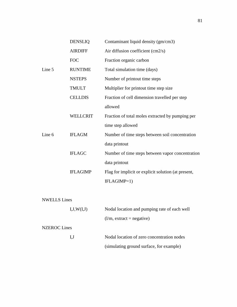
DATA INPUT FORMAT
All numbers are read by the program in free format, so position and decimal
digits are unimportant for individual variables. An ASCII data file is constructed
thus:
Line number Variable name Description
Line 1 TITLE Simulation title
Line 2 NX Number of columns (NX<21)
DX Column width (cm)
NY Number of rows (NY<21)
DY Row width (cm)
THCK Thickness in third dimension (cm)
POR Total Porosity (vol. fraction) (0<POR<1)
MOIST Soil moisture (vol. fraction) (0<MOIST<POR)
NWELLS Number of wells
NZEROC Number of constant conc. cells (for diffusion)
Line 3 SDENS Soil density (gm/cm3)
TEMP Simulation temperature (oC)
OMEGA Flow iteration acceleration parameter
(1<OMEGA<2)
CRIT Flow iteration criteria (percent)
RH Relative humidity of incoming air (0<RH<1)
RHINJ Relative humidity of injected air (0<RHINJ<1)
CINJ Concentration of injected air (mole/cm3)
Line 4 NCOMP Number of compounds (NCOMP<50)
81
DENSLIQ Contaminant liquid density (gm/cm3)
AIRDIFF Air diffusion coefficient (cm2/s)
FOC Fraction organic carbon
Line 5 RUNTIME Total simulation time (days)
NSTEPS Number of printout time steps
TMULT Multiplier for printout time step size
CELLDIS Fraction of cell dimension travelled per step
allowed
WELLCRIT Fraction of total moles extracted by pumping per
time step allowed
Line 6 IFLAGM Number of time steps between soil concentration
data printout
IFLAGC Number of time steps between vapor concentration
data printout
IFLAGIMP Flag for implicit or explicit solution (at present,
IFLAGIMP=1)
NWELLS Lines
I,J,W(I,J) Nodal location and pumping rate of each well
(l/m, extract = negative)
NZEROC Lines
I,J Nodal location of zero concentration nodes
(simulating ground surface, for example)
82
What follows are the arrays for permeability, surface leakage, and initial total
contaminant concentration distribution. Each array starts with one line specifying
whether the array is homogeneous anf can be described by one value (FACTOR). If
not, then an array follows and each value is multiplied by the number FACTOR. The
arrays are as follows:
Intrinsic permeability:
Line 1 INFLAG (if INFLAG=1, INTRK array follows, and is x
FACTOR. If INFLAG=0, all INTRK(I,J)=
FACTOR) (darcy).
FACTOR see above
Plus or minus Intrinsic permeability array
Vertical leakage permeability:
Line 1 INFLAG (if INFLAG=1, VPERM array follows, and is
x FACTOR. If INFLAG=0, all VPERM(I,J)=
FACTOR) (darcy).
FACTOR see above
OVERBRDN thickness of leaky confining layer (feet)
Plus or minus confining bed vertical permeability
Initial concentration array:
Line 1 INFLAG (if INFLAG=1, C array follows, and is x
FACTOR. If INFLAG=0, all C(I,J)=
FACTOR) (darcy).
FACTOR see above
83
Plus or minus Initial concentration array
NCOMP Lines of
MASSF(N) mass fraction of compound n (dimensionless)
MW(N) molecular weight of compound n (gm/mol)
BP(N) boiling point of compound n (degrees C)
VP(N) vapor pressure of compound n at 20oC (ATM)
SOL(N) solubity of compound n (mg/l)
KD(N) octanol/water partition coefficient of compound n
ICOMPFL(N) flag specifying whether to print concentrations of
compound n at every printout time step (0=do not
print, 1=print)
NCOMP Lines of
LCNAME(N) the name of compound n
84
APPENDIX C
SAMPLE INPUT AND OUTPUT FILES
85
The following is a sample data input file, and the corresponding output is listed
UNSPECIFIED PLASTICS MANUFACTURER - TRACK ETHYLBENZENE 6 COLUMNS AT 304.8 CM EACH 6 ROWS AT 304.8 CM EACHTHICKNESS IN 3RD DIMENSION = 609.6 CMTOTAL POROSITY = 0.40FRACTION ORGANIC C = 0.00NUMBER OF COMPOUNDS = 6FREE AIR DIFFUSION = 0.084 CM2/SEC
INITIAL CONTAMINANT COMPOSITION AND PHYSICAL PROPERTIES
MASS BALANCE CALCULATIONS AT TIME = 0.00 DAYS PUMPED MASS DIFF. LOSS MASS REMAINING INITIAL MASS MASS ERROR (%) ERROR (%) 0.0000E+00 0.0000E+00 0.3040E+07 0.3040E+07 0.000E+00 ?????????
REMAINING TOTAL CONC. (MG/KG) AT TIME = 300.68 DAYS
MASS BALANCE CALCULATIONS AT TIME = 300.68 DAYS PUMPED MASS DIFF. LOSS MASS REMAINING INITIAL MASS MASS ERROR (%) ERROR (%) -.1933E+07 0.0000E+00 0.1107E+07 0.3040E+07 0.152E-01 0.391E-01
REMAINING TOTAL CONC. (MG/KG) AT TIME = 661.71 DAYS
MASS BALANCE CALCULATIONS AT TIME = 661.71 DAYS PUMPED MASS DIFF. LOSS MASS REMAINING INITIAL MASS MASS ERROR (%) ERROR (%) -.2643E+07 0.0000E+00 0.3982E+06 0.3040E+07 0.292E-01 0.628E-01
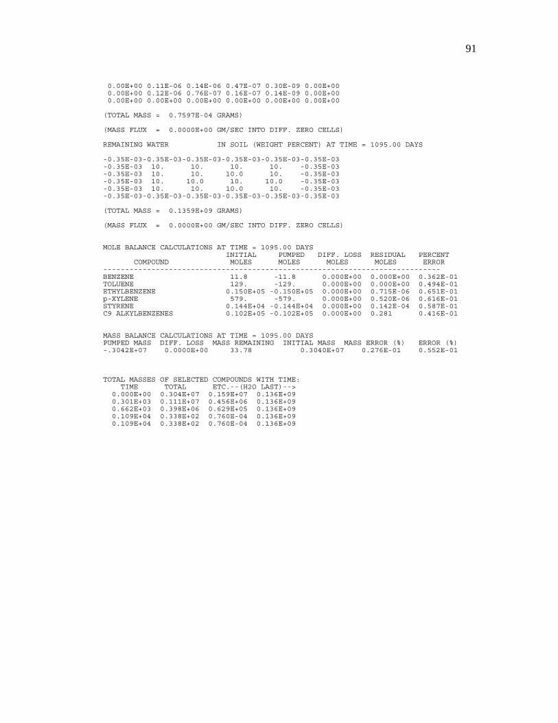
REMAINING TOTAL CONC. (MG/KG) AT TIME = 1094.99 DAYS
MASS BALANCE CALCULATIONS AT TIME = 1094.99 DAYS PUMPED MASS DIFF. LOSS MASS REMAINING INITIAL MASS MASS ERROR (%) ERROR (%) -.3042E+07 0.0000E+00 33.79 0.3040E+07 0.276E-01 0.552E-01
REMAINING TOTAL CONC. (MG/KG) AT TIME = 1095.00 DAYS
MASS BALANCE CALCULATIONS AT TIME = 1095.00 DAYS PUMPED MASS DIFF. LOSS MASS REMAINING INITIAL MASS MASS ERROR (%) ERROR (%) -.3042E+07 0.0000E+00 33.78 0.3040E+07 0.276E-01 0.552E-01
TOTAL MASSES OF SELECTED COMPOUNDS WITH TIME: TIME TOTAL ETC.--(H2O LAST)--> 0.000E+00 0.304E+07 0.159E+07 0.136E+09 0.301E+03 0.111E+07 0.456E+06 0.136E+09 0.662E+03 0.398E+06 0.629E+05 0.136E+09 0.109E+04 0.338E+02 0.760E-04 0.136E+09 0.109E+04 0.338E+02 0.760E-04 0.136E+09
92
ABSTRACT
93
ABSTRACT
Prediction of the transport of volatile mixtures within unsaturated soils can be
complicated by the interaction of chemical compounds with variable physical
properties. The analysis and design of vapor-extraction remedial systems depends on
models which can simulate the chemical and physical factors which affect the
removal of vapor-phase chemical mixtures, such as gasoline. Present models fall into
two categories: 1) non-dimensional (no transport), multi-compound phase distribution
models or 2) multi-dimensional, single-compound transport models. In this paper, a
numerical simulation is presented which couples the steady-state vapor flow equation,
the parabolic advection-diffusion transport equation, and a multiple-compound, four-
phase equilibrium model. The simulation allows spatially variable fields of
permeability, surface leakage, and initial contaminant concentrations. The user can
specify the location and discharge rates of any number of extraction or injection wells,
including zero wells, in which case the simulation will solve transport by diffusion
only. The utility of the model is shown by solving hypothetical gasoline spill
remediation by vapor extraction when the natural conditions are non-ideal. The non-
ideal conditions include inhomogeneous soil permeability, irregular surface leakage
(from fill areas or surface seals), and irregular contaminant distribution. The model is
also run in the pure diffusion mode to show the limitations of three-phase (no
separate-phase), single-compound vapor flux models in predicting chemical fate and