Numerical Analysis and Scientific Computing Preprint Seria A two-energies principle for the biharmonic equation and an a posteriori error estimator for an interior penalty discontinuous Galerkin approximation D. Braess R. H. W. Hoppe C. Linsenmann Preprint #48 Department of Mathematics University of Houston March 2016
Transcript
Numerical Analysis and Scientific Computing
Preprint Seria
A two-energies principle for the
biharmonic equation and an a posteriori
error estimator for an interior penalty
discontinuous Galerkin approximation
D. Braess R. H. W. Hoppe C. Linsenmann
Preprint #48
Department of Mathematics
University of Houston
March 2016
A TWO-ENERGIES PRINCIPLE FOR THE BIHARMONICEQUATION AND AN A POSTERIORI ERROR ESTIMATOR FOR
AN INTERIOR PENALTY DISCONTINUOUS GALERKINAPPROXIMATION
D. BRAESS⇤, R. H. W. HOPPE‡§ , AND C. LINSENMANN†
Abstract. We consider an a posteriori error estimator for the Interior Penalty DiscontinuousGalerkin (IPDG) approximation of the biharmonic equation based on the Hellan-Herrmann-Johnson(HHJ) mixed formulation. The error estimator is derived from a two-energies principle for the HHJformulation and amounts to the construction of an equilibrated moment tensor which is done by localinterpolation. The reliability estimate is a direct consequence of the two-energies principle and doesnot involve generic constants except for possible data oscillations. The e�ciency of the estimatorfollows by showing that it can be bounded from above by a residual-type estimator known to bee�cient. A documentation of numerical results illustrates the performance of the estimator.
1. Introduction. The biharmonic equation is more often solved by nonconform-ing or mixed methods than by conforming elements in order to avoid the computation-ally expensive implementation of H2 conforming elements such as the Argyris plateelements of the TUBA family [4] or the generalizations of the Hsieh–Clough–Tocherelements from [20]. As far as mixed methods are concerned, the fourth order equationis written as a system of two second order equations, e.g.,
D2u = p,
r ·r · p = f,(1.1)
where D2u is the matrix of second partial derivatives of u and p stands for the mo-
ment tensor. The formulation (1.1) leads to the mixed method of Hellan–Herrmann–Johnson [30, 31, 33]. Another splitting is given by
�u = w,�w = f,
(1.2)
and leads to the mixed method of Ciarlet–Raviart [17]. Among nonconforming ap-proaches, Discontinuous Galerkin (DG) methods have been studied recently in [14,15, 26, 27, 28] (for other fourth order problems see [21, 42]). The relationship betweenDG methods and mixed methods turns out to be useful for the biharmonic problemas it is for second order elliptic boundary value problems due to the unified analysisin [6]. Fourth order problems have been treated similarly in [27].
⇤Faculty of Mathematics, Ruhr-University, D-44780 Bochum, GermanyE-mail: [email protected]
‡Inst. of Math., Univ. of Augsburg, D-86159 Augsburg, GermanyE-mail: [email protected]
§Dept. of Math., Univ. of Houston, Houston, TX 77204-3008, U.S.A.E-mail: [email protected]
§Supported by NSF grants DMS-1115658, DMS-1216857, DMS-1520886, and by the DFG withinthe Priority Program SPP 1506.
†Inst. of Math., Univ. of Augsburg, D-86159 Augsburg, GermanyE-mail: [email protected]
1
The Interior Penalty DG (IPDG) methods considered in [27, 28] rely on the Ciarlet–Raviart mixed formulation (1.2). They are fully discontinuous in the sense that glob-ally discontinuous, piecewise polynomials of degree k � 2 are used for the approxi-mation of the primal variable u. On the other hand, those in [14, 15, 26] are basedon the Hellan–Herrmann–Johnson splitting as given by (1.1). The IPDG schemes in[14, 15, 26] feature C0 elements of Lagrangian type. Residual-type a posteriori errorestimators have been considered and analyzed in [14, 26], and [28].
We will consider a posteriori error bounds by the two-energies principle, also knownas the hypercircle method. It was originally developed by Prager and Synge [36, 38,39] and more recently considered in connection with second order elliptic problemsin [1, 7, 8, 9, 10, 11, 12, 41]. The considerations of DG methods in this direction[2, 3, 18, 22, 23, 24, 25] were also done for equations of second order.
In this paper, we focus on the biharmonic equation in the formulation of Hellan–Herrmann–Johnson and the application of the hypercircle method to its IPDG ap-proximation. The advantage of a posteriori error bounds based on the two-energiesprinciple compared to standard residual-type error estimators is that the reliabilityestimate does not contain generic constants except for possible oscillation terms (seethe papers mentioned above and (5.8) below). As we shall see, the implementationamounts to the construction of an equilibrated moment tensor which can be done bymeans of a discrete three-field mixed formulation of the IPDG approximation. Theconstruction only requires local interpolations in a postprocessing. Nevertheless, theanalysis is more involved than the analogous one for equations of second order.
The paper is organized as follows: Section 2 lists some notation. In Section 3, weintroduce the two-energies principle for the Hellan–Herrmann–Johnson mixed formu-lation (1.1). Section 4 is devoted to the IPDG approximation and associated discretetwo-field and three-field formulations. Section 5 describes how the error bounds ob-tained from the two-energies principle can be built into a reliable a posteriori errorestimator. The construction of the equilibrated moment tensor is dealt with in Sec-tion 6. In Section 7, we prove the e�ciency of the estimator by showing that it canbe bounded from above by a residual-type estimator which is known to be e�cient.Finally, in Section 8 we provide a documentation of numerical results illustrating thequasi-optimality of the IPDG approximation and the performance of the estimator.
2. Notation. We will use standard notation from Lebesgue and Sobolev spacetheory [8, 13, 40]. In particular, for a bounded domain ⌦ ⇢ R2 and D ✓ ⌦ wedenote the L2-inner product and the associated L2-norm by (·, ·)0,D and k · k0,D,respectively. We further refer to Hk(⌦), k 2 N, as the Sobolev spaces with innerproduct (·, ·)k,⌦, norm k ·kk,⌦, and seminorm | · |k,⌦, and to Hk�1/2(�0),�0 ✓ � = @⌦,as the associated trace spaces. Hk
0 (⌦) stands for the closure of C10 (⌦) in theHk-norm.
Further, H�k(⌦) refers to the dual space of Hk0 (⌦) with h·, ·ik,⌦ denoting the dual
product. Moreover,H(div,⌦) is the Hilbert space of vector fields q 2 L2(⌦)2 such thatr ·q 2 L2(⌦). Matrix-valued functions in L2(⌦)2⇥2 will be denoted by q = (qij)2i,j=1
and the inner-product is (p,q)0,⌦ :=R
⌦ p : q dx, where p : q :=P2
i,j=1 pijqij .
Further, we introduce the Hilbert space
H(div2,⌦) := {q 2 H(div,⌦)2 | r · q 2 H(div,⌦)}.
Finally, given a function u 2 H2(⌦), we refer to D2u := (@2u/@xi@xj)2i,j=1 as thematrix of second partial derivatives.
2
Let Th(⌦) be a geometrically conforming, locally quasi-uniform simplicial triangula-tion of the computational domain. For D ✓ ⌦, we denote by Eh(D) the set of edgesof Th(⌦) in D. We further denote by hK ,K 2 Th(⌦), the diameter of K and byhE , E 2 Eh(⌦), the length of E. Moreover, for D ✓ K we refer to Pm(D), m 2 N, asthe set of polynomials of degree m on D. Due to the local quasi-uniformity of thetriangulation, there exist constants 0 < c C such that
c hE hK C hE , E 2 Eh(@K). (2.1)
For a function w 2 L2(⌦) with w|K 2 C(K),K 2 Th(⌦), and an interior edge E =K+\K�, K± 2 Th(⌦), we set w± := w|E\K± and define the average and jump acrossE as usual according to
{w}E :=
⇢
12 (w+ + w�) , E 2 Eh(⌦)
w|E , E 2 Eh(�), (2.2a)
[w]E :=
⇢
w+ � w� , E 2 Eh(⌦)w|E , E 2 Eh(�)
. (2.2b)
The average and jump across E 2 Eh(⌦) are defined analogously for vector fieldsw 2 L2(⌦)2 with w|K 2 C(K)2,K 2 Th(⌦), and tensors p 2 L2(⌦)2⇥2 with p|K 2C(K)2⇥2,K 2 Th(⌦). Moreover, we refer to nE , E 2 Eh(⌦), E = K+ \ K�, as theunit normal vector pointing from K+ to K� and to nE , E 2 Eh(�), as the exteriorunit normal vector n� on E \ �. Products like
[w]EnE = w+n@K+ + w�n@K�
and other products under consideration are independent of the choice of K+ and K�and the resulting orientation of the edge.
3. A two-energies principle for the biharmonic equation. Given a boundedpolygonal domain ⌦ ⇢ R2 with boundary � := @⌦ and a function f 2 H�2(⌦), weconsider the biharmonic problem
�2u = f in ⌦, (3.1a)
u = n� ·ru = 0 on �. (3.1b)
A primal variational formulation of (3.1) amounts to the computation of u 2 H20 (⌦)
such that for all v 2 H20 (⌦) it holds
(D2u,D2v)0,⌦ = hf, vi2,⌦. (3.2)
It is well-known that (3.2) represents the optimality condition for the following un-constrained minimization problem: Find u 2 H2
0 (⌦) such that
Jp(u) = infv2H2
0 (⌦)Jp(v),
where the primal energy functional Jp : H20 (⌦) ! R is given by
Jp(v) :=1
2(D2v,D2v)0,⌦ � hf, vi2,⌦. (3.3)
3
In order to specify the associated dual problem, the divergence of a matrix-valuedfunction q = (qij)2i,j=1 with row vectors q(i) = (qi1, qi2)T , 1 i 2, is defined as
usual
r · q := (r · q(1),r · q(2))T . (3.4)
The dual or complementary energy Jd : L2(⌦)2⇥2 ! R , given by
Jd(q) := �1
2(q,q)0,⌦,
will be maximized subject to the constraint
(q, D2v)0,⌦ = hf, vi2,⌦ for all v 2 H20 (⌦). (3.5)
The relation (3.5) may be understood as
r ·r · q = f in H�2(⌦)
or in the distributional sense.
Theorem 3.1. Let Jp and Jd be defined as above. Then
minv2H2
0
Jp(v) = maxq2L2(⌦)2⇥2
�
Jd(q) | r ·r · q = f
(3.6)
where the constraint on the right-hand side of (3.6) is understood as in (3.5).
Proof. By definition we have for v and q as in (3.6)
Jp(v)� Jd(q) =1
2(D2v,D2v)0,⌦ � hf, vi2,⌦ +
1
2(q,q)0,⌦
=1
2(D2v � q, D2v � q)0,⌦ + (q, D2v)0,⌦ � (f, v)0,⌦
=1
2kD2v � qk0,⌦ � 0,
since the relation (3.5) holds by assumption. It follows that inf Jp(v) � sup Jd(q)
where the infimum and the supremum are understood in the spirit of (3.6). Since wehave equality for v := u and q := D2u, the proof is complete.
We are now in a position to state an abstract version of the two-energies principle forthe biharmonic equation; cf. [35, Theorem 3.1].
Theorem 3.2. (Two-energies principle for the biharmonic equation)Let u 2 H2
0 (⌦) be the solution of (3.2), and let p 2 L2(⌦)2⇥2 satisfy the equilibrium
Proof. We provide a short proof for completeness. If u 2 H20 (⌦) is the solution of
(3.2), then (D2u,D2(v � u))0,⌦ = hf, v � u)i2,⌦. Next we conclude from (3.5) that
the equilibrium assumption (3.7) implies (p, D2(v � u))0,⌦ = hf, v � ui2,⌦. Hence,
(D2u� p, D2(u� v))0,⌦ = hf � f, u� vi2,⌦ = 0.
An application of the binomial formula to k(D2v�D2u)+ (D2u�p)k20,⌦ yields (3.8).
The relationship (3.8) is called the two-energies principle, because it can be stated interms of the primal energy Jp(v) and the complementary energy Jd(p) as
kD2(v � u)k20,⌦ + kD2u� pk20,⌦ = 2�
Jp(v)� Jd(p)�
.
We conclude this section with a formulation of the two-energies principle that is bettermanageable in finite element computations. In particular, it translates the equilibriumcondition (3.7) for f 2 L2(⌦) from H�2 to an element-wise property. We considermoment tensors p 2 L2(⌦)2⇥2 that satisfy
p|K 2 Pk(K)2⇥2, k � 2, K 2 Th(⌦), (3.9a)
[p]E nE = 0, E 2 Eh(⌦), (3.9b)
nE · [r · p]E = 0, E 2 Eh(⌦). (3.9c)
The propertiest (3.9) imply p 2 H(div2,⌦) (but are not necessary). This is obvious
from (3.11) in the proof of the announced version of the two-energies principle.
Theorem 3.3. (Variant of the two-energies principle) Let u 2 H20 (⌦) be the solution
of (3.2) for f 2 L2(⌦). Moreover, for a geometrically conforming simplicial triangu-lation Th(⌦) of ⌦ let p 2 H(div2,⌦) satisfy (3.9a)–(3.9c) as well as the equilibrium
condition
r ·r · p = f in each K 2 Th(⌦). (3.10)
Then, for v 2 H20 (⌦) it holds
kD2v � pk20,⌦ = kD2(v � u)k20,⌦ + kD2u� pk20,⌦.
Proof. Using (3.2) and applying integration by parts, we obtainZ
⌦
(D2u� p) : D2(u� v) dx =
Z
⌦
f (u� v) dx�X
K2Th(⌦)
Z
K
p : D2(u� v) dx (3.11)
=X
K2Th(⌦)
Z
K
(f �r ·r · p) (u� v) dx�X
K2Th(⌦)
Z
@K
p n@K ·r(u� v) ds
+X
K2Th(⌦)
Z
@K
n@K ·r · p (u� v) ds,
5
where n@K is the outward unit normal on @K. The first term in the second line of(3.11) vanishes due to (3.10), whereas the boundary integrals vanish due to (3.9b),(3.9c)and u� v = n@K ·r(u� v) = 0 on @K \ �. Hence, it follows that
Z
⌦
(D2u� p) : D2(u� v) dx = 0.
The assertion is again an immediate consequence of this orthogonality relation.
4. An IPDG approximation of the biharmonic equation. We considerthe interior penalty discontinuous Galerkin (IPDG) approximation of the biharmonicproblem (3.2) with f 2 L2(⌦) on a geometrically conforming, locally quasi-uniformsimplicial triangulation Th(⌦) of the computational domain. It involves element-wisepolynomial approximations of u. For k � 2 we introduce the IPDG space
as well as the space of element-wise polynomial moment tensors
Mh:= {q
h2 L2(⌦)2⇥2 | q
h|K 2 Pk(K)2⇥2, K 2 Th(⌦)}. (4.2)
We define a bilinear form aIPh (·, ·) : Vh ⇥ Vh ! R for the variational IPDG approxi-mation
aIPh (uh, vh) :=X
K2Th(⌦)
Z
K
D2uh : D2vh dx (4.3)
+X
E2Eh(⌦)
Z
E
⇣
nE · {r ·D2uh}E [vh]E + [uh]E nE · {r ·D2vh}E⌘
ds
�X
E2Eh(⌦)
Z
E
⇣
[ruh]E · {D2vh}E nE + [rvh]E · {D2uh}E nE
⌘
ds
+X
E2Eh(⌦)
Z
E
↵1
hEnE · [ruh]E nE · [rvh]E ds+
X
E2Eh(⌦)
Z
E
↵2
h3E
[uh]E [vh]E ds,
where ↵i > 0, i = 1, 2, are suitable penalty parameters. The IPDG approximation of(3.2) reads: Find uh 2 Vh such that
aIPh (uh, vh) = (f, vh)0,⌦, vh 2 Vh. (4.4)
Remark 4.1. The Hellan–Herrmann–Johnson based symmetric IPDG approximation(4.4) is the counterpart of the Ciarlet–Raviart based symmetric IPDG approximationin [27, 28]. If we would choose the finite element space Vh = Vh \ C0(⌦), then itreduces to the symmetric C0IPDG approximation considered in [14, 15], and [26]. Inthe C0 case the last sum in (4.3) vanishes and is abandoned there.
For completeness, we note that aIPh (·, ·) is not well defined for functions in H20 (⌦).
This can be cured by means of a lifting operator
L : Vh +H20 (⌦) ! M
hZ
⌦
L(v) : qhdx =
X
E2Eh(⌦)
Z
E
⇣
[v]E nE · {r · qh}E � [rv]E · {q
h}EnE
⌘
ds. (4.5)
6
The lifting operator L is stable in the sense that it satisfies (cf. [27])
kL(v)k20,⌦ .X
E2Eh(⌦)
⇣
h�1E knE · [rv]Ek20,E + h�3
E k[v]Ek20,E⌘
, v 2 Vh +H20 (⌦).
Now we define aIPh : (Vh +H20 (⌦))⇥ (Vh +H2
0 (⌦)) ! R as follows:
aIPh (u, v) :=X
K2Th(⌦)
Z
K
⇣
D2u : D2v + (L(u) : D2v +D2u : L(v))⌘
dx (4.6)
+X
E2Eh(⌦)
Z
E
↵1
hEnE · [ru]E nE · [rv]E ds+
X
E2Eh(⌦)
Z
E
↵2
h3E
[u]E [v]E ds.
It is easy to verify that aIPh (uh, vh) = aIPh (uh, vh) holds for uh, vh 2 Vh.
We introduce the mesh-dependent IPDG norm on Vh +H20 (⌦)
kvk22,h,⌦ :=X
K2Th(⌦)
kD2vk20,K (4.7)
+X
E2Eh(⌦)
↵1
hEknE · [rv]Ek20,E +
X
E2Eh(⌦)
↵2
h3E
k[v]Ek20,E .
It is not di�cult to show that for su�ciently large penalty parameters ↵i, i = 1, 2,i.e., ↵1 = O((k + 1)2),↵2 = O((k + 1)6), there exists a positive constant � such that
aIPh (v, v) � � kvk22,h,⌦, v 2 Vh +H20 (⌦). (4.8)
On the other hand, there exists a constant � > 1 such that for any ↵i > 0, 1 i 2,
In particular, it follows from (4.8) and (4.9) that the IPDG approximation (4.4) admitsa unique solution uh 2 Vh for su�ciently large penalty parameters.
A mixed formulation in the spirit of [6] was given in [27] for the Ciarlet–Raviartmethod. We provide now two mixed Hellan–Herrmann–Johnson type formulations of(4.4) by specifying appropriate numerical flux functions on the edges E 2 Eh(⌦)
bu(1) :=
(
{ruh}E , E 2 Eh(⌦)0, E 2 Eh(�)
, (4.10a)
u(2) :=
(
{uh}E , E 2 Eh(⌦)0, E 2 Eh(�)
, (4.10b)
bp := {D2uh}E � ↵1
hEnE [ruh]
TE , (4.10c)
b := {r ·D2uh}+↵2
h3E
[uh]E nE . (4.10d)
We keep the notion numerical fluxes from [6] although not all the variables in (4.10)are fluxes in the strict sense.
7
The mixed method with the two-field-formulation reads as follows: Find (uh,ph) 2
Vh⇥Mhand numerical fluxes such that (4.10a)–(4.10d) holds and simultaneously for
all (v,q) 2 Vh ⇥Mhand K 2 Th(⌦)
Z
K
ph: q dx�
Z
K
uh r ·r · q dx (4.11a)
�Z
@K
bu(1) · q n@K ds+
Z
@K
u(2)nE ·r · q ds = 0,
Z
K
ph: D2v dx�
Z
@K
bpn@K ·rv ds (4.11b)
+
Z
@K
n@K · b v ds =
Z
K
f v dx.
All the equations are coupled since they contain equations on elements as well as onedges.
Often another implementation is considered as more convenient. – First the solutionuh of the primal method is determined by solving linear equations with a positivedefinite matrix. The numerical fluxes are determined immediately by their definition(4.10). The moment tensor p
hcan be evaluated by solving the small linear system
(4.11a) for each K 2 Th.
Lemma 4.2. Let the numerical flux functions bu(1), u(2), bp and b , be given by (4.10)
and suppose that the penalty parameters ↵i, 1 i 2, are su�ciently large.
(i) If uh 2 Vh is the unique solution of (4.4), then there exists ph2 M
hsuch that
the pair (uh,ph) satisfies (4.11).
(ii) If (uh,ph) 2 Vh⇥M
his a solution of (4.11), then uh is the solution of the IPDG
approximation (4.4).
Proof. Let uh 2 Vh be the unique solution of (4.4). The associated numerical fluxesare known from (4.10). We define p
h2 M
hby means of (4.11a). Next, letK 2 Th(⌦)
and v 2 Vh. We apply (4.11a) with q(x) = D2v(x), x 2 K, and insert the expressions
(4.10a), (4.10b) for the numerical fluxes to obtain
Z
K
ph: D2v dx =
Z
K
uh r ·r ·D2v dx (4.12)
+
Z
@K
{ruh}@K ·D2v n@K ds�Z
@K
{uh}@K n@K ·r ·D2v ds.
Using Green’s formula
Z
K
uh r ·r ·D2hv dx =
Z
K
D2huh : D2
hv dx (4.13)
�Z
@K
ruh ·D2v n@K ds+
Z
@K
uhn@K ·r ·D2v ds,
for eliminating the first integral on the right-hand side of (4.12) we get
8
Z
K
ph: D2v dx (4.14)
=
Z
K
D2huh : D2
hv dx�Z
@K
ruh ·D2v n@K ds+
Z
@K
uhn@K ·r ·D2v ds
+
Z
@K
{ruh}@K ·D2v n@K ds�Z
@K
{uh}@K n@K ·r ·D2v ds.
We recall that {w}@K � w|@K = 12 [w]@K . Summation over all triangles yields
X
K2Th(⌦)
Z
K
ph: D2v dx =
X
K2Th(⌦)
Z
K
D2huh : D2
hv dx (4.15)
+X
E2Eh(⌦)
Z
E
[ruh]E · {D2v}EnE ds�X
E2Eh(⌦)
Z
E
[uh]E nE · {r ·D2v}E ds.
Next, we use the variational equality (4.4) to eliminate the first integral on theright.hand side of (4.15),
X
K2Th(⌦)
Z
K
ph: D2v dx (4.16)
=X
E2Eh(⌦)
Z
E
⇣
{nE ·r ·D2uh}E [v]E + [uh]E nE · {r ·D2v}E⌘
ds
�X
E2Eh(⌦)
Z
E
⇣
[ruh]E · {D2v nE}E + {D2uh nE}E · [rv]E⌘
ds
�X
E2Eh(⌦)
Z
E
↵1
hE[nE ·ruh]E [nE ·rv]E ds�
X
E2Eh(⌦)
Z
E
↵2
h3E
[uh]E [v]E ds
+
Z
⌦
fv dx
+X
E2Eh(⌦)
Z
E
[ruh]E · {D2v}EnE ds�X
E2Eh(⌦)
Z
E
[uh]E nE ·r · {D2v}E ds.
Note that four integrals in (4.16) cancel. Observing (4.10c),(4.10d) we obtain (4.11b).
Conversely, if (uh,ph) 2 Vh ⇥ M
hsolves (4.11a), (4.11b), we choose q := D2v in
(4.11a). Applying Green’s formula (4.13) again, we can eliminate phfrom the system.
It follows that uh is a solution of the primal problem (4.4) which proves (ii).
Instead of the two-field formulation (4.11) we consider next a three-field formulationby introducing the finite element space
W h := {�h2 L2(⌦)2 | �
h|K 2 Pk�1(K)2,K 2 Th(⌦)}. (4.17)
The three-field formulation reads as follows: Find (uh,ph,
h) 2 Vh ⇥ M
h⇥ W h
together with the numerical flux functions bu(1), u(2), bp and b in (4.10) such that for
9
all (v,q,�) 2 Vh ⇥Mh⇥W h and all K 2 Th(⌦) it holds
Z
K
ph: q dx�
Z
K
uh r ·r · q dx (4.18a)
�Z
@K
bu(1) · q n@K ds+
Z
@K
u(2)n@K ·r · q ds = 0,Z
K
ph: r� dx�
Z
@K
bpn@K · � ds = �Z
K
h· � dx, (4.18b)
Z
K
h·rv dx�
Z
@K
n@K · b v ds = �Z
K
fv dx. (4.18c)
Lemma 4.3. Under the assumptions of Lemma 4.2 it holds:
(i) If uh 2 Vh is the unique solution of (4.4), then there exists a unique pair(p
h,
h) 2 M
h⇥W h such that the triple (uh,p
h,
h) satisfies (4.18).
(ii) If (uh,ph,
h) 2 Vh ⇥M
h⇥W h is a solution of (4.18), then the pair (uh,p
h)
solves (4.11), and uh is the solution of the IPDG approximation (4.4).
Proof. If uh 2 Vh is the unique solution of (4.4), we already know from Lemma 4.2(i)that there exists p
h2 M
hsuch that (4.11a) and (4.11b) are satisfied. Next, we
define h2 W h by means of (4.18b). Choosing � = rv we may replace the first
two terms in (4.11b) byP
K
R
K
h·rv dx. It follows that (4.18c) holds true which
proves (i).
Conversely, if (uh,ph,
h) 2 Vh⇥M
h⇥W h is a solution of (4.18a)–(4.18c), obviously
(4.11a) and (4.18a) coincide. Next, we set � = rv in (4.18b) and evaluate the termin the second line via (4.18c),
X
K2Th(⌦)
Z
K
ph: D2v dx�
X
K2Th(⌦)
Z
@K
bpn@K ·rv ds
= �X
K2Th(⌦)
Z
K
h·rv dx,
= �X
K2Th(⌦)
Z
@K
n@K · b v ds+X
K2Th(⌦)
Z
K
fv dx.
Hence, we obtain (4.11b). Now Lemma 4.2, part (ii) shows that uh solves (4.4) whichproves (ii).
5. An a posteriori error estimator for the IPDG approximation of thebiharmonic equation. The construction of an equilibrated moment tensor in thefinite element framework will be a↵ected by data oscillation, and the case k = 2requires special care. This will be clear from Remark 6.5 below. Specifically, set
Meq
h:= {q
h2 L2(⌦)2⇥2 | q
h|K 2 P`(K)2⇥2, K 2 Th(⌦)}, (5.1)
where ` :=
(
k if k � 3,
3 if k = 2.
10
Given K 2 Th(⌦), let fK be the L2-projection of f onto P`�2(K), and let fh 2 L2(⌦)be given by fh|K = fK ,K 2 Th(⌦). A moment tensor peq
h2 Meq
his called equilibrated
in this framework, if if satisfies (3.9b),(3.9c) which implies peq
h2 H(div2,⌦), and also
the equilibrium equation
r ·r · peq
h= fh in each K 2 Th(⌦). (5.2)
The two-energies principle (Theorem 3.3) can be applied to the IPDG approximation(4.4) involving an equilibrated moment tensor peq
h. It gives rise to an a posteriori
error bound in terms of element-related terms ⌘eqK,i, 1 i 2, and edge-related terms⌘eqE,i, 1 i 2, as given by
⌘eqK,1 := kD2uh � peq
hk0,K , K 2 Th(⌦), (5.3a)
⌘eqK,2 := kD2uh �D2uconfh k0,K , K 2 Th(⌦), (5.3b)
0 (⌦) in (5.3b) will be constructed by postprocessing from the finiteelement solution uh 2 Vh.
The following auxiliary result deals with the data oscillation due to the approximationof f by fh. Its application is not restricted to a posteriori error estimates.
Lemma 5.1. Let z 2 H20 (⌦) be the weak solution of the biharmonic problem
�2z = f � fh in ⌦, (5.4a)
z = n� ·rz = 0 on � = @⌦. (5.4b)
If the L2-projection of f � fh to P1(K) in each K 2 Th vanishes, then
kD2zk20,⌦ CX
K2Th(⌦)
h4K kf � fhk20,K . (5.5)
Proof. For v 2 H20 (⌦) and p1 2 P1(K),K 2 Th(⌦), we have by assumptionX
K2Th(⌦)
(D2z,D2v)0,K =X
K2Th(⌦)
(f � fh, v � p1)0,K .
Choosing v = z, it follows thatX
K2Th(⌦)
kD2zk20,K X
K2Th(⌦)
kf � fhk0,K kz � p1k0,K .
We fix p1 2 P1(K) by the interpolation conditionsR
Kp1dx =
R
Kzdx and
R
Krp1dx =
R
Krzdx. The Poincare-Friedrichs inequalities (cf., e.g., [34])
kz � p1k0,K ChK
⇣
krzk0,K +�
�
�
Z
K
(z � p1) dx�
�
�
⌘
,
kr(z � p1)k0,K ChK
⇣
kD2zk0,K +�
�
�
Z
K
r(z � p1) dx�
�
�
R2
⌘
.
11
yield the relationX
K2Th(⌦)
kD2zk20,K C2X
K2Th(⌦)
kD2zk0,Kh2Kkf � fhk0,K .
By applying the Cauchy inequality to the right-hand side and dividing by the squareroot of the left-hand side we obtain the assertion.
The data oscillation will be denoted by
osc2h(f) :=X
K2Th(⌦)
osc2K(f), osc2K(f) := h4K kf � fhk20,K . (5.6)
The error bound in the following theorem refers to the norm (4.7).
Theorem 5.2. Let u 2 H20 (⌦) be the solution of the biharmonic problem (3.1a),
(3.1b), let uh 2 Vh be the unique solution of the IPDG approximation (4.4), and letpeq
h2 Meq
h\ H(div2,⌦) be an equilibrated moment tensor. Moreover, let uconf
h 2H2
0 (⌦), let ⌘eqK,i, ⌘
eqE,i, 1 i 2, be given by (5.3a)–(5.3d), and let osch(f) be the data
oscillation (5.6). We set
⌘eqh :=⇣
X
K2Th(⌦)
(⌘eqK,1)2⌘1/2
+ 2⇣
X
K2Th(⌦)
(⌘eqK,2)2⌘1/2
(5.7)
+⇣
X
E2Eh(⌦)
(↵1(⌘eqE,1)
2 + ↵2(⌘eqE,2)
2)⌘1/2
.
Then there exists a constant C1 > 0, which only depends on the local geometry of thetriangulation, such that it holds
ku� uhk2,h,⌦ ⌘eqh + C1 osch(f). (5.8)
Proof. Let u 2 H20 (⌦) be the weak solution of the biharmonic problem
�2u = fh in ⌦,
u = n� ·ru = 0 on � = @⌦.
By recalling (4.7) and applying the triangle inequality twice we obtain
ku� uhk2,h,⌦ (5.9)
⇣
X
K2Th(⌦)
kD2u�D2uhk20,K⌘1/2
+⇣
X
E2Eh(⌦)
(↵1(⌘eqE,1)
2 + ↵2(⌘eqE,2)
2)⌘1/2
⇣
X
K2Th(⌦)
kD2u�D2uk20,K⌘1/2
+⇣
X
K2Th(⌦)
kD2u�D2uconfh k20,K
⌘1/2
+⇣
X
K2Th(⌦)
kD2uconfh �D2uh)k20,K
⌘1/2+⇣
X
E2Eh(⌦)
(↵1(⌘eqE,1)
2 + ↵2(⌘eqE,2)
2)⌘1/2
.
Since z := u � u solves (5.4a),(5.4b), the first term in the third line of (5.9) can beestimated from above by Lemma 5.1 and thus gives rise to the data oscillation term in
12
(5.8). The two-energies principle (Theorem 3.3) with u = u, v = uconfh and p = peq
hyields
kD2(u� uconfh )k0,⌦
⇣
X
K2Th(⌦)
kD2uconfh � peq
hk20,K
⌘1/2 (5.10)
⇣
X
K2Th(⌦)
⇣
kD2uh �D2uconfh k20,K
⌘1/2+⇣
X
K2Th(⌦)
kpeq
h�D2uhk20,K
⌘1/2.
Using these estimates in (5.9) allows to conclude.
Remark 5.3. We note that the constant C1 in front of the data oscillation termosch(f) is the only generic constant occurring in the reliability estimate (5.8).
In practice, a modified equilibrated error estimator avoids the computationally ex-pensive evaluation of uconf
h and attracts attention, although the reliability estimate(5.11) below contains another generic constant.
Corollary 5.4. Assume that the assumptions of Theorem 5.2 are satisfied. Specif-ically, let V conf
h be the generalized version of the classical Hsieh–Clough–Tocher C 1
conforming finite element space as constructed in [20], and let uconfh = Eh(uh) be the
extension of uh to V confh as defined in [28]. Then there exists a constant C2 > 0, de-
pending only on the local geometry of the triangulation and on the penalty parameters↵i, 1 i 2, such that it holds
ku� uhk2,h,⌦ (5.11)⇣
X
K2Th(⌦)
(⌘eqK,1)2⌘1/2
+ C2
⇣
X
E2Eh(⌦)
((⌘eqE,1)2 + (⌘eqE,2)
2)⌘1/2
+ C osch(f).
Proof. In [28] it has been shown that
X
K2Th(⌦)
(⌘eqK,2)2 .
X
E2Eh(⌦)
((⌘eqE,1)2 + (⌘eqE,2)
2). (5.12)
Using (5.12) in (5.8) yields (5.11).
6. Construction of an equilibrated moment tensor. We construct an equi-librated moment tensor peq
h2 Meq
h\H(div2,⌦) which allows to apply the two-energies
principle and Theorem 5.2. The construction will be done by an interpolation on eachelement. Thus it is a local procedure. In particular, denoting by BDMm(K),m 2 N,the Brezzi-Douglas-Marini element of polynomial degreem (cf., e.g., [16]), we first con-struct an auxiliary vector field eq
h2 H(div,⌦), eq
h|K 2 BDM`�1(K),K 2 Th(⌦),
satisfying
r · eq
h= fh in L2(⌦), (6.1)
and then an equilibrated moment tensor peq
h2 Meq
h\H(div2,⌦) satisfying
r · peq
h= eq
hin L2(⌦)2. (6.2)
13
For the construction of the auxiliary vector field we recall the following result:
Lemma 6.1. Let m � 1. Any vector field � 2 Pm(K) is uniquely defined by thefollowing degrees of freedom
Z
E
nE · � q ds, q 2 Pm(E), E 2 Eh(@K), (6.3a)Z
K
� ·rq dx, q 2 Pm�1(K), (6.3b)Z
K
� · curl(bKq) dx, q 2 Pm�2(K). (6.3c)
where bK in (6.3c) is the element bubble function on K given by bK =3Q
i=1�Ki and
�Ki , 1 i 3, are the barycentric coordinates of K. Moreover, there exists a positive
constant C1(m) depending only on the polynomial degree m and the local geometry ofthe triangulation Th(⌦) such that
Z
K
|�|2 dx C1(k)⇣
X
E2Eh(@K)
hE
Z
E
|nE · �|2 ds+ h2K
Z
K
|r · �|2 dx (6.4)
+ h2K max
�
Z
K
|� · curl(bKq)|2 dx; q 2 Pm�2(K), maxx2K
|q(x)| 1
⌘
.
Proof. For the uniqueness result we refer to (3.41) in [16, p. 125] since BDMm(K) =Pm(K). The estimate (6.4) can be derived by standard scaling arguments (cf. Lemma3.1 and Remark 3.3 in [9]).
The auxiliary vector field eq
his constructed in each element K 2 Th such that
eq
h|K 2 BDM`�1(K) satisfies the interpolation conditions
Z
E
nE · eq
hq ds =
Z
E
nE · b q ds, q 2 P`�1(E), E 2 Eh(@K), (6.5a)
Z
K
eq
h·rq dx =
Z
K
h·rq dx, q 2 P`�2(K), (6.5b)
Z
K
eq
h· curl(bKq) dx =
Z
K
r ·D2uh · curl(bKq) dx, q 2 P`�3(K). (6.5c)
Lemma 6.2. The vector field eq
hthat is defined by (6.5) is contained in H(div,⌦)
and satisfies (6.1).
Proof. The solvability of (6.5a)–(6.5c) is guaranteed by Lemma 6.1 with m = ` � 1.The continuity of the normal components follows from (6.5a) on adjacent trianglesand yields eq
h2 H(div,⌦).
Let K 2 Th(⌦). Given a polynomial q 2 P`�2 ⇢ Pk, we can use (4.18c) with v|K = qand vh|K0 = 0, K 6= K 0 2 Th(⌦). Moreover we make use of Green’s formula, as well
14
as of (6.5a) and (6.5b) to obtain
Z
K
r · eq
hq dx = �
Z
K
eq
h·rq dx+
Z
@K
n@K · eq
hq ds
= �Z
K
h·rq dx+
Z
@K
n@K · b q ds
=
Z
K
fq dx =
Z
K
fhq dx.
Since both r · eq
hand fh live in P`�2(K), (6.1) follows from the preceding equation.
Now, the assertion follows from eq
h2 H(div,⌦).
The construction (6.5) by local interpolation and Lemma 6.2 take into account thatthere is a compatibility condition due to Gauss’ theorem. The divergence of eq
hin
K cannot be fixed independently of the normal components of eq
hon @K, but the
latter are required in order to achieve the continuity of the normal components and eq
h2 H(div,⌦).
The compatibility conditions are satisfied here due to the finite element equation(4.18c) for the discontinuous Galerkin (IPDG) method. They enable us to proceedon elements like e.g., in [9, 18, 22], and we need not operate on patches like in theapplications of the two-energies principle and H1-conforming elements as, e.g., in[10, 12] or [8, Section III.9].
For the construction of the equilibrated moment tensor peq
hwe begin with the speci-
fication of the degrees of freedom for tensors p 2 P`(K)2⇥2.
Lemma 6.3. We have dim P`(K)2⇥2 = 2(` + 1)(` + 2). Any p 2 P`(K)2⇥2, p =
(pij)2i,j=1, with p(i) := (pi1, pi2)T , 1 i 2, is uniquely determined by the followingdegrees of freedom (DOF)
Z
E
(p nE) · q ds, q 2 P`(E)2, E 2 Eh(@K)., (6.6a)Z
K
p : rq dx, q 2 P`�1(K)2\P0(K)2, (6.6b)Z
K
p(i) · curl(bKq) dx, q 2 P`�2(K), 1 i 2. (6.6c)
The numbers of degrees of freedom (DOF) associated with (6.6a)–(6.6c) are as follows
DOF (6.6a) = 6(`+ 1),
DOF (6.6b) = `(`+ 1)� 2,
DOF (6.6c) = `(`� 1)
and sum up to 2(`+ 1)(`+ 2).
Proof. The interpolation conditions for p(1) and p(2) are separated. The vector field
15
p(i) (for 1 i 2) is determined by the degrees of freedom
Z
E
p(i) nE q ds, q 2 P`(E), E 2 Eh(@K).,Z
K
p(i) ·rq dx, q 2 P`�1(K)\P0(K),Z
K
p(i) · curl(bKq) dx, q 2 P`�2(K) .
By applying Lemma 6.1 with m = ` we conclude that there is a unique solution.
Lemma 6.4. Let q = (q(1),q(2)) 2 P`(K)2⇥2. Then there exists a positive con-
stant C2(`) depending only on the polynomial degree ` and the local geometry of thetriangulation Th(⌦) such that
Z
K
|q|2 dx C2(k)⇣
X
E2Eh(@K)
hE
Z
E
(|nE · qnE |2 + |tE · qnE |2) ds (6.7)
+ h2K
Z
K
|r · q|2 dx
+ h2K
2X
i=1
maxn
Z
K
|q(i) · curl(bKq`�2)|2 dx; q`�2 2 P`�2,maxx2K
|qk�2(x)| 1o⌘
.
Proof. As in the proof of Lemma 6.1, the estimate (6.7) follows by standard scalingarguments.
Now, for the construction of the equilibrated moment tensor we set zh:= D2uh with
z(1)h := (@2uh
@x21
,@2uh
@x1@x2)T , z(2)h := (
@2uh
@x1@x2,@2uh
@x22
)T .
We construct peq
h= (ph,eqij )2i,j=1, with p(i)
h,eq = (ph,eqi1 , ph,eqi2 )T , 1 i 2, in each
element K by fixing the degrees of freedom (6.6a)–(6.6c) according to
Z
E
peq
hnE · q ds =
Z
E
bp nE · q ds, q 2 P`(E)2, E 2 Eh(@K), (6.8a)
Z
K
peq
h: rq dx = �
Z
K
eq
h· q dx+
Z
@K
bpn@K · q ds, q 2 P`�1(K)2 (6.8b)
Z
K
p(i)h,eq
· curl(bKq) dx =
Z
K
z(i)h · curl(bKq) dx, q 2 P`�2(K), 1 i 2. (6.8c)
Remark 6.5. Obviously, the equations (6.8b) require the compatibility conditions
�Z
K
eq
h· p dx+
Z
@K
bpn@K · p ds = 0, p 2 P0(K)2 (6.9)
16
with constant polynomials p 2 P0(K)2. Indeed, we had to care for ` � 3 in (5.1) inorder to verify (6.9) now. From the finite element equation (4.18b) we conclude that
�Z
K
h· p dx+
Z
@K
bpn@K · p ds = 0, p 2 P0(K)2.
Given p = (p1, p2) 2 P0(K)2, there exists q 2 P1(K) with p = rq, specifically(p1, p2) = r(p1x1 + p2x2). Since ` � 3, we conclude from (6.5b) that
Z
K
eq
h· p dx =
Z
K
eq
h·rq dx =
Z
K
h·rq dx =
Z
K
h· p dx.
Combining the last two equations we obtain (6.9)
The following theorem is the main result and shows that peq
his an equilibrated moment
tensor and thus fulfills all requirements of the two-energies principle.
Theorem 6.6. Let k � 2. If the moment tensor peq
hand the auxiliary vector field eq
h
are constructed by (6.8) and (6.5), respectively, then peq
h2 H(div2,⌦) is equilibrated,
i.e.,
r ·r · peq
h= fh in L2(⌦).
Proof. It follows from (6.8a) that the normal components of peq
hare continuous on
edges. Hence, peq
h2 H(div2,⌦) Let K 2 Th(⌦). From Remark 6.5 we know that the
compatibility condition (6.9) is satisfied. We apply partial integration and insert therules (6.8a), (6.8b) for the construction of peq
hto obtain
Z
K
r · peq
h· q dx = �
Z
K
peq
h: rq dx+
Z
@K
peq
hn@K · q ds (6.10)
= �⇣
�Z
K
eq
h· q dx+
Z
@K
bpn@K · q ds⌘
+
Z
@K
bpn@K · q ds
=
Z
K
eq
h· q dx , q 2 P`�1(K)2.
Since both r · peq
hand eq
hlive in P`�1(K)2, it follows from (6.10) that
r · peq
h= eq
h. (6.11)
The left-hand side is contained in H(div,⌦) since it holds for the right-hand side dueto Lemma 6.2. Moreover it follows that peq
h2 H(div2,⌦) and
r ·r · peq
h= r · eq
h= fh
and the proof is complete.
Usually mixed methods for the treatment of the Hellan–Herrrmann–Johnson for-mulation use finite elements for the moment tensors that are H(div2) nonconform-ing. This is due to the fact that no simple conforming elements are known. The
17
reader will have observed that the equilibrated moment tensors are constructed inM
h\ H(div2,⌦). Thus we have implicitly an H(div2)-conforming finite element
space. We conclude from the e�ciency considerations in the next section that thisfinite element (sub)space is su�ciently large.
Remark 6.7. We note that the divergence of a tensor was defined row-wise in (3.4).If we had chosen a column-wise definition, then we would have obtained the trans-posed tensor peq,T
hof the result (6.8). It follows that also peq,T
h2 H(div2,⌦) and
div divpeq,T
h= fh. Therefore we may use also the symmetrical part
peq,sym
h=
1
2
�
peq
h+ peq,T
h
�
for computing the term (5.3a) of the error bound, i.e.,
⌘eq,sK,1 := kD2uh � peq,sym
hk0,K , K 2 Th(⌦). (6.12)
Since the symmetrical part and the antisymmetrical part of a tensor are L2-orthogonal,it follows that
⌘eq,sK,1 ⌘eqK,1, K 2 Th(⌦). (6.13)
Indeed, numerical results below show that the error bound can be reduced by about 30%in this way.
7. E�ciency of the equilibrated error estimator. A residual-type a posteri-ori error estimator has been derived and analyzed in [28] for the IPDG approximationof the biharmonic problem. It is based on the Ciarlet–Raviart mixed formulation,and its adaptation to the Hellan–Hermann–Johnson based IPDG approximation (4.4)reads as follows:
(⌘resh )2 =X
K2Th(⌦)
(⌘resK )2 +X
E2Eh(⌦)
⇣
(⌘resE,1)2 + (⌘resE,2)
2 + (⌘resE,c)2⌘
, (7.1)
where the element residual ⌘resK and the edge residuals ⌘resE,1, ⌘resE,2, ⌘
resE,c are given by
(⌘resK )2 := h4K kf ��2uhk20,K , (7.2)
(⌘resE,1)2 := h3
E knE · [r�uhk20,E ,
(⌘resE,2)2 := hE
⇣
knE · [D2uh]E nEk20,E + ktE · [D2uh]E nEk20,E⌘
,
(⌘resE,c)2 := h�1
E knE · [ruh]Ek20,E + h�3E k[uh]Ek20,E .
A slight generalization of the e�ciency estimate from [28] shows
(⌘resh )2 . ku� uhk22,h,⌦ + osc2h(f). (7.3)
The e�ciency of the equilibrated a posteriori error estimator ⌘eqh follows from (7.3)and the following result.
Lemma 7.1. Let ⌘eqK ,K 2 Th(⌦), and osch(f) be given by (5.3a) and (5.6), and let⌘resh be the residual-type a posteriori error estimator (7.1). Then there holds
X
K2Th(⌦)
(⌘eqK,1)2 . (⌘resh )2 + osc2h(f). (7.4)
18
Proof. Let K 2 Th(⌦) and E 2 Eh(@K). Due to (6.8a) and (4.10c) we have peq
Due to (7.8) and (7.9a),(7.9b), an application of Lemma 6.1 to eq
h� r · D2uh 2
P`�1(K)2 yields
k eq
h�r ·D2uhk20,K . h2
K kfh ��2uhk20,K + (7.10)
X
E2Eh(@K)
hE knE · [r�uh]Ek20,E +X
E2Eh(@K)
↵22
h3E
k[uh]Ek20,E .
Using the local quasi-uniformity once more, we have hE ⇠ hK for E 2 Eh(@K) andestimate the bounds above in terms of the residual estimators (7.2)
h2Kk eq
h�r ·D2uhk20,K . (⌘resE,2)
2 + h4Kkf � fhk20,K +
X
E2Eh(@K)
⇣
(⌘resE,2)2 + (⌘resE,3)
2⌘
.
We insert this bound into (7.7), sum over all K 2 Th(⌦), and the proof is complete.
Theorem 7.2. Let u 2 H20 (⌦) be the solution of the biharmonic problem (3.1), and
let uh 2 Vh be the IPDG approximation. Moreover, let ⌘eqK,i, ⌘eqE,i, 1 i 2, and
osch(f) be given by (5.3a)–(5.3c) and (5.6). Then there exists a constant C > 0depending on the polynomial degree k, the local geometry of the triangulation, and onthe penalty parameters ↵i, 1 i 2, such that
X
K2Th(⌦)
⇣
(⌘eqK,1)2 + (⌘eqK,2)
2⌘
+X
E2Eh(⌦)
((⌘eqE,1)2 + (⌘eqE,2)
2) (7.11)
C⇣
ku� uhk22,h,⌦ + osc2h(f)⌘
.
Proof. The assertion follows directly from (5.12), (7.3), and (7.4).
Since the residual a posteriori error estimator is known to be e�cient [28], the errorbounds from the two-energies principle are also e�cient.
20
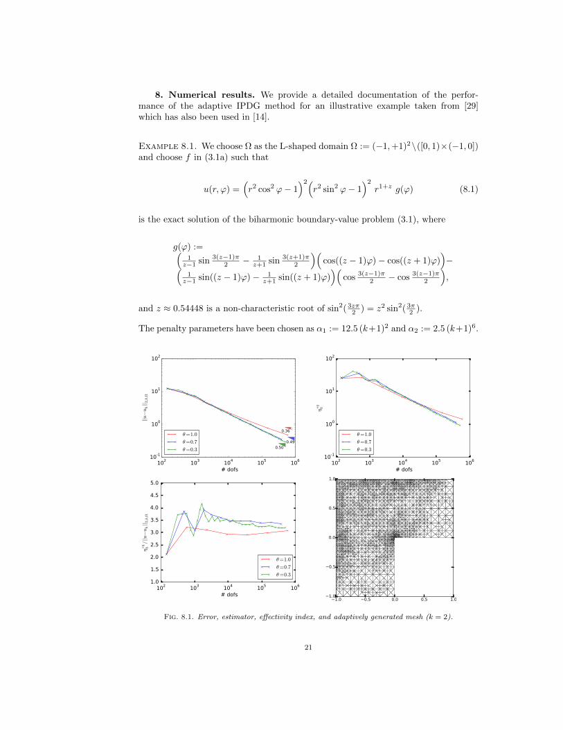
8. Numerical results. We provide a detailed documentation of the perfor-mance of the adaptive IPDG method for an illustrative example taken from [29]which has also been used in [14].
Example 8.1. We choose ⌦ as the L-shaped domain ⌦ := (�1,+1)2\([0, 1)⇥(�1, 0])and choose f in (3.1a) such that
u(r,') =⇣
r2 cos2 '� 1⌘2⇣
r2 sin2 '� 1⌘2
r1+z g(') (8.1)
is the exact solution of the biharmonic boundary-value problem (3.1), where
g(') :=⇣
1z�1 sin
3(z�1)⇡2 � 1
z+1 sin3(z+1)⇡
2
⌘⇣
cos((z � 1)')� cos((z + 1)')⌘
�⇣
1z�1 sin((z � 1)')� 1
z+1 sin((z + 1)')⌘⇣
cos 3(z�1)⇡2 � cos 3(z�1)⇡
2
⌘
,
and z ⇡ 0.54448 is a non-characteristic root of sin2( 3z⇡2 ) = z2 sin2( 3⇡2 ).
The penalty parameters have been chosen as ↵1 := 12.5 (k+1)2 and ↵2 := 2.5 (k+1)6.
where ⌘eq,sK,1 has been defined in (6.12). Note that the re-definition of ⌘eqh in (8.2b)di↵ers from (5.7) in so far as we have omitted the second term of the right-hand sidein (5.7) because according to (5.12) it can be estimated from above by the third term.
For polynomial degree 2 k 5 and bulk parameters ✓ = 1.0 (uniform refinement),✓ = 0.7, and ✓ = 0.3 Figures 8.1–8.4 display
• the global discretization error u � uh in the mesh-dependent IPDG-normk · k2,h,⌦ (top left) and the error estimator ⌘eqh (top right) as a function of thetotal number of degrees of freedom (dofs) on a logarithmic scale,
• the associated e↵ectivity index ⌘eqh /ku� uhk2,h,⌦ (bottom left),• the adaptively generated mesh (✓ = 0.7) at refinement level 7 for k = 2, level
9 for k = 3, level 11 for k = 4, and level 13 for k = 5 (bottom right).
We observe a significant refinement in a vicinity of the reentrant corner where thesolution has a singularity and some refinement in regions near the upper and left
boundary segments of the computational domain where second derivatives of the so-lution have local peaks. As expected, the refinement is less pronounced for higherpolynomial degree k. Moreover, for k = 2 the beneficial e↵ect of adaptive refinementsets in for a total number of DOFs (# DOFs) exceeding 104, whereas for 3 k 5it occurs for # DOFs ⇡ 103 and is much more pronounced than for k = 2. Thee↵ectivity index is between 2.0 and 4.5 for all polynomial degrees 2 k 5.We note that the computation of the equilibrated moment tensor is ill-conditioned.The condition number deteriorates significantly with decreasing mesh size and in-creasing polynomial degree k. For k = 4 and k = 5, Figures 8.3 and 8.4 only displaythe results up to refinement levels before roundo↵ errors have an influence on thenumerical results.
Table 8.1 lists results of the computation for k = 3 and ✓ = 0.3 and addresses certaincomponents of the error estimator ⌘eqh . By using the symmetrical part ⌘eq,sh (cf.(8.2c)) as suggested in Remark 6.7, the error bounds and therefore also the associatede↵ectivity indices ⌘eq,sh /ku � uhk2,h,⌦ can be reduced by 15 to 20%. The weightededge-related terms as given by ⌘eqEh,↵
contribute only about 12 � 15% to the overallerror estimator.
[1] M. Ainsworth and J.T. Oden, Posteriori Error Estimation in Finite Element Analysis. Wiley,Chichester, 2000.
[2] M. Ainsworth and R. Rankin, Fully computable error bounds for discontinuous Galerkin finite
24
element approximations on meshes with an arbitrary number of levels of hanging nodes.SIAM J. Numer. Anal. 47, 4112–4141, 2010
[3] M. Ainsworth and R. Rankin, Constant free error bounds for non-uniform order discontinuousGalerkin finite element approximation on locally refined meshes with hanging nodes. IMAJ. Numer. Anal. 31, 254–280, 2011.
[4] J.H. Argyris, I. Fried, and D.W. Scharpf, The TUBA family of plate elements for the matrixdisplacement method. Aero. J. Roy. Aero. Soc., 72, 701–709, 1968.
[5] D. Arnold and F. Brezzi, Mixed and nonconforming finite element methods: implementation,postprocessing and error estimates. M2AN 19, 7–32, 1985.
[6] D. Arnold, F. Brezzi, B. Cockburn, and D. Marini, Unified analysis of discontinuous Galerkinmethods for elliptic problems. SIAM J. Numer. Anal. 39, 1749–1779, 2002.
[7] I. Babuska and T. Strouboulis, The Finite Element Method and its Reliability. Clarendon Press,Oxford, 2001.
[8] D. Braess, Finite Elements, Theory, Fast Solvers and Applications in Solid Mechanics. 3rdedition. Cambridge University Press, Cambridge, 2007.
[9] D. Braess, T. Fraunholz, and R.H.W. Hoppe, An equilibrated a posteriori error estimator forthe interior penalty discontinuous Galerkin method. SIAM J. Numer. Anal. 52, 2121-2136,2014.
[10] D. Braess, R.H.W. Hoppe, and J. Schoberl, A posteriori estimators for obstacle problems bythe hypercircle method. Comp. Visual. Sci. 11, 351–362, 2008.
[11] D. Braess, V. Pillwein, and J. Schoberl, Equilibrated residual error estimates are p-robust.Comp. Meth. Applied Mech. Engrg. 198, 1189–1197, 2009.
[12] D. Braess and J. Schoberl, Equilibrated residual error estimator for edge elements. Math. Comp.77, 651–672, 2008.
[13] S.C. Brenner and L. Ridgway Scott, The Mathematical Theory of Finite Element Methods. 3rdEdition. Springer, New York, 2008
[14] S.C. Brenner, T. Gudi, and L.-Y. Sung, An a posteriori error estimator for a quadratic C0-interior penalty method for the biharmonic problem. IMA J. Numer. Anal., 30, 777–798,2010.
[15] S.C. Brenner and L.-Y. Sung, C0 interior penalty methods for fourth order elliptic boundaryvalue problems on polygonal domains. J. Sci. Comput., 22/23, 83–118, 2005.
[16] F. Brezzi and M. Fortin, Mixed and Hybrid Finite Element Methods. Springer, Berlin-Heidelberg-New York, 1991.
[17] P.G. Ciarlet and P.-A. Raviart, A mixed finite element method for the biharmonic equation.In: Mathematical Aspects of Finite Elements in Partial Di↵erential Equations (C. de Boor,ed), pp. 125–145. Academic Press, New York, 1974.
[18] S. Cochez-Dhondt and S. Nicaise, Equilibrated error estimators for discontinuous Galerkinmethods. Numer. Methods Partial Di↵er. Equations 24, 1236–1252, 2008.
[19] W. Dorfler, A convergent adaptive algorithm for Poisson’s equation. SIAM J. Numer. Anal.33, 1106–1124, 1996.
[20] J. Douglas Jr., T. Dupont, P. Percell, and R. Scott, A family of C1 finite elements with optimalapproximation properties for various Galerkin methods for 2nd and 4th order problems.RAIRO Anal. Numer. 13, 227–255, 1979.
[21] G. Engel, K. Garikipati, T.J.R Hughes, M.G. Larson, L. Mazzei, and R.L. Taylor, Continu-ous/discontinuous finite element approximations of fourth order elliptic problems in struc-tural and continuum mechanics with applications to thin beams and plates, and straingradient elasticity. Comput. Methods Appl. Mech. Engrg. 191, 3669–3750, 2002.
[22] A. Ern, S. Nicaise, and M. Vohralık, An accurate H(div) flux reconstruction for discontinuousGalerkin approximations of elliptic problems. C. R. Acad. Sci. Paris Ser. I 345, 709–712,2007.
[23] A. Ern and A. F. Stephansen, A posteriori energy-norm error estimates for advection-di↵usionequations approximated by weighted interior penalty methods. J. Comput. Math. 26, 488–510, 2008.
[24] A. Ern, A. F. Stephansen, and M. Vohralık, Guaranteed and robust discontinuous Galerkina posteriori error estimates for convection-di↵usion-reaction problems. J. Comput. Appl.Math. 234, 114–130, 2010.
[25] A. Ern and M. Vohralık, Flux reconstruction and a posteriori error estimation for discontinuousGalerkin methods on general nonmatching grids. C. R. Acad. Sci. Paris Ser. I 347, 4441–4444, 2009.
[26] T. Fraunholz, R.H.W. Hoppe, and M. Peter, Convergence analysis of an adaptive interiorpenalty discontinuous Galerkin method for the biharmonic problem. J. Numer. Math. 23,311–330, 2015.
25
[27] E.H. Georgoulis and P. Houston, Discontinuous Galerkin methods for the biharmonic problem.IMA J. Numer. Anal. 29, 573–594, 2009.
[28] E.H. Georgoulis, P. Houston, and J. Virtanen, An a posteriori error indicator for discontinuousGalerkin approximations of fourth order elliptic problems. IMA J. Numer. Anal. 31, 281–298, 2011.
[29] P. Grisvard, Elliptic Problems in Nonsmooth Domains. Pitman, Boston-London-Melbourne,1985.
[30] K. Hellan, Analysis of elastic plates in flexure by a simplified finite element method. ActaPolytechnica Scandinavia, Civil Engineering Series 46, 1967.
[31] L. Herrmann, Finite element bending analysis for plates. J. Eng. Mech. Div. A.S.C.E. EM5 93,13–26, 1967.
[32] R.H.W. Hoppe, G. Kanschat, and T. Warburton, Convergence analysis of an adaptive interiorpenalty discontinuous Galerkin method. SIAM J. Numer. Anal., 47, 534–550, 2009.
[33] C. Johnson, On the convergence of a mixed finite element method for plate bending problems.Numer. Math. 21, 43–62, 1973.
[34] J. Necas, Les Methodes Directes en Theorie des Equations Elliptiques. Masson, Paris, 1967.[35] P. Neittaanmaki and S. Repin, A posteriori error estimates for boundary-value problems related
to the biharmonic equation. East-West J. Numer. Math. 9, 157–178, 2001[36] W. Prager and J.L. Synge, Approximations in elasticity based on the concept of function spaces.
Quart. Appl. Math. 5, 241–269, 1947.[37] E. Suli and I. Mozolevski, hp-version interior penalty DGFEMs for the biharmonic equation.
Comput. Methods Appl. Mech. Eng. 196, 1851–1863, 2007.[38] J.L. Synge, The method of the hypercircle in function-space for boundary-value problems. Proc.
Royal Soc. London, Ser. A 191, 447–467, 1947.[39] J.L. Synge, The Hypercircle Method in Mathematical Physics: A Method for the Approximate
Solution of Boundary Value Problems. Cambridge University Press, New York, 1957.[40] L. Tartar, Introduction to Sobolev Spaces and Interpolation Theory. Springer, Berlin–
Heidelberg–New York, 2007.[41] T. Vejchodsky, Local a posteriori error estimator based on the hypercircle methof. In: Proceed-
ings ECCOMAS 2004 (P. Neittaanmaki et al., eds.), 16 pages, University of Jyvaskyla,Jyvaskyla, 2004.
[42] G.N. Wells, E. Kuhl, and K. Garikipati, A discontinuous Galerkin method for the Cahn-Hilliardequation. J. Comp. Phys. 218, 860–877, 2006.