A two-layer shallow water model for bedload sedimenttransport: convergence to Saint-Venant-Exner model

C. Escalante ∗, E.D. Fernandez-Nieto †,T. Morales de Luna ‡, G. Narbona-Reina†

November 13, 2017

Abstract

A two-layer shallow water type model is proposed to describe bedload sedimenttransport. The upper layer is filled by water and the lower one by sediment. The keypoint falls on the definition of the friction laws between the two layers, which are ageneralization of those introduced in Fernandez-Nieto et al. (ESAIM: M2AN, 51:115-145, 2017). This definition allows to apply properly the two-layer shallow water modelfor the case of intense and slow bedload sediment transport. Moreover, we provethat the two-layer model converges to a Saint-Venant-Exner system (SVE) includinggravitational effects when the ratio between the hydrodynamic and morphodynamictime scales is small. The SVE with gravitational effects is a degenerated nonlinearparabolic system. This means that its numerical approximation is very expensivefrom a computational point of view, see for example T. Morales de Luna et al. (J. Sci.Comp., 48(1): 258–273, 2011). In this work, gravitational effects are introduced intothe two-layer system without such extra computational cost. Finally, we also considera generalization of the model that includes a non-hydrostatic pressure correction forthe fluid layer and the boundary condition at the sediment surface. Numerical testsshow that the model provides promising results and behave well in low transport rateregimes as well as in many other situations.

∗Dpto. de A.M., E. e I.O., y Matematica Aplicada - Universidad de Malaga, Campus de Teatinos s/n.29071 Malaga, Spain. (escalante@uma.es)†Dpto. Matematica Aplicada I. ETS Arquitectura - Universidad de Sevilla. Avda. Reina Mercedes N.

2. 41012-Sevilla, Spain. (edofer@us.es), (gnarbona@us.es)‡Dpto. de Matematicas. Universidad de Cordoba. Campus de Rabanales. 14071 Cordoba, Spain.

(tomas.morales@uco.es)

1

arX

iv:1

711.

0359

2v1

[ph

ysic

s.fl

u-dy

n] 8

Nov

201

7

1 Introduction

One of the difficulties to simulate bedload sediment transport is that the interaction be-tween fluid and sediment is very small. Bedload is the type of transport where sedimentgrains roll along the bed or single grains jump over the bed a length proportional to theirdiameter, losing for instants the contact with the soil. This is opposed to transport insuspension where particles are transported by the fluid without touching the bottom forlong period of times. For low Froude numbers, bedload is the dominating transport mech-anism. In this case the characteristic velocities of fluid and sediment are very different.The bedload transport rate is low and the characteristic velocity of the sediment is muchsmaller than that of the fluid.

In [13], a multi-scale analysis is performed taking into account that the velocity of thesediment layer is smaller than the one of the fluid layer. This leads to a shallow water typesystem for the fluid layer and a lubrication Reynolds equation for the sediment one.

For the case of uniform flows the thickness of the moving sediment layer can be pre-dicted, because erosion and deposition rates are equal in those situations. This is a generalhypothesis that is assumed when modeling bedload transport. The usual approach is toconsider a coupled system consisting of a Shallow Water system for the hydrodynamicalpart combined with a morphodynamical part given by the so-called Exner equation. Thewhole system is known as Saint Venant Exner (SVE) system [9]. Exner equation dependson the definition of the solid transport discharge. Different classical definitions can be foundfor the solid transport discharge, for instance the ones given by Meyer-Peter & Muller [21],Van Rijn’s [35], Einstein [6], Nielsen [23], Fernandez-Luque & Van Beek [10], Ashida &Michiue [1], Engelund & Fredsoe [8], Kalinske [18], Charru [4], etc. A generalization ofthese classical models was introduced in [13] where the morphodynamical component isdeduced from a Reynolds equation and includes gravitational effects in the sediment layer.Classical models do not take into account in general such gravitational effects because intheir derivation the hypothesis of nearly horizontal sediment bed is used (see for example[19]).In general, classical definitions for solid transport discharge can be written as follows,

qbQ

= sgn(τ)k1

(1− ϕ)θm1 (θ − k2 θc)

m2+

(√θ − k3

√θc

)m3

+, (1)

where Q represents the characteristic discharge, Q = ds√g(1/r − 1)ds, r = ρ1/ρ2 is the

density ratio, ρ1 being the fluid density and ρ2 the density of the sediment particles; ds themean diameter of the sediment particles, and ϕ is the averaged porosity. The coefficientskl and ml, l = 1, 2, 3, are positive constants that depend on the model. We usually findm2 = 0 or m3 = 0, for example, Meyer-Peter & Muller model takes m3 = 0 and Ashida &Michiue’s model uses m2 = 0.The Shields stress, θ, is defined as the ratio between the agitating and the stabilizingforces, θ = |τ |d2

s/(g(ρ2 − ρ1)d3s), τ being the shear stress at the bottom. For example, for

Manning’s law, we have τ = ρ1gh1n2u1|u1|/h4/3

1 . Where h1 and u1 are the thickness andthe velocity of the fluid layer, respectively, and n is the Manning coefficient.

2

Finally, θc is the critical Shields stress. The positive part, ( · )+, in the definition impliesthat the solid transport discharge is not null only if θ > kθc (with k = k2 when m2 > 0 andk =√k3 when m3 > 0). If the velocity of the fluid is zero, u1 = 0, we have θ = 0 < kθc,

and for any model that can be written under the structure (1) we obtain that qb = 0,which means that there is no movement of the sediment layer. This is even true when thesediment layer interface is not horizontal which is a consequence of the fact that classicalmodels do not take into account gravitational effects.

In order to introduce gravitational effects in classical models, Fowler et al. proposed in[14] a modification of the Meyer-Peter & Muller formula that consist in replacing θ by θeff,where:

θeff = |sgn(u1)θ − ϑ∂x(b+ h2)| , (2)

with

ϑ =θc

tan δ, (3)

δ being the angle of repose of the sediment particles. The sediment surface is defined byz = b+h2, where h2 is the thickness of the sediment layer and b the topography function orbedrock layer. Then, θeff is defined in terms of the gradient of sediment surface. This is adefinition that can be also considered for 2D simulations, because in this case θeff is definedas the norm of the vector θu1/‖u1‖−ϑ∇(b+h2). Other alternatives have been proposed inthe literature, namely consisting of a modification of θc, instead of a modification of θ. Bothapproximations are equivalent only in some cases for 1D problems (see [13]). Moreover,defining the modification of θc for arbitrarily sloping bed for 2D problems is not an easytask (see [24], [29]).

As we mentioned previously, in [13] a SVE model is deduced from a multiscale analysis.The model includes gravitational effects and the authors deduce that it can also be seenas a modification of classical models by replacing θ by the proposed values θ

(L)eff or θ

(Q)eff

depending if we set a linear or a quadratic friction law respectively between the fluid andthe sediment layer. For the case of nearly uniform flows, the thickness of the sediment layerwhich corresponds to moving particles, hm, is of order of ds/ϑ. Under this assumption, forthe case of a linear friction law, the definition of the effective shear stress proposed in [13]can be written as follows:

θ(L)eff =

∣∣∣∣sgn(u1)θ − ϑ∂x(b+ h2)− ϑ ρ1

ρ2 − ρ1

∂x(b+ h1 + h2)

∣∣∣∣ . (4)

Let us remark that if the water free surface is horizontal, the definition of θ(L)eff coincides

with θeff (2), proposed by Fowler et al. in [14]. Otherwise, the main difference is thatthis definition for the effective shear stress takes into account not only the gradient of thesediment surface but also the gradient of the water free surface.

For the case of a quadratic friction law, although the definition is a combination ofthe same components, it is rather different. In this case we can write the effective Shields

3

parameter proposed in [13] as follows:

θ(Q)eff =

∣∣∣∣∣sgn(u1)√θ −

√ϑρ1

ρ2 − ρ1

|∂x(ρ1

ρ2

h1 + h2 + b)| sgn

(∂x(

ρ1

ρ2

h1 + h2 + b)

)∣∣∣∣∣2

. (5)

In the case of submerged bedload sediment transport, the drag term is defined by aquadratic friction law. Thus, we should consider an effective Shields stress given by θ

(Q)eff .

Nevertheless, in the bibliography it is θeff (2) which is usually considered, regardless the

fact that θeff is an approximation of θ(L)eff which is deduced from a linear friction law.

Although the quantities involved in the definitions of the effective Shields parameterassociated to linear or quadratic friction are the same, their values may be very different.They verify

|θ(L)eff − θ

(Q)eff | = O

(|∂x(

ρ1

ρ2

h1 + h2 + b)|

(√θ −

√ϑρ1

ρ2 − ρ1

|∂x(ρ1

ρ2

h1 + h2 + b)|

)).

For instance, if we consider a initial condition with water at rest and a high gradient inthe sediment surface, the difference between θ

(L)eff and θ

(Q)eff is of order of the gradient of

the sediment surface. Thus, in the framework of SVE model, the definition θ(Q)eff should be

considered in order to be consistent with the quadratic friction law usually considered forthe drag force between the fluid and the sediment.

In any case, considering the definitions θeff (2), θ(L)eff (4), or θ

(Q)eff (5), means that the

corresponding SVE system with gravitational effects is a parabolic degenerated partialdifferential system with non linear diffusion. Moreover, the system cannot be written ascombination of a hyperbolic part plus a diffusion term.

Let us remark that in the literature a linearized version can be found, where gravita-tional effects are included by considering a classical SVE model with an additional viscousterm, see for example [33] and references therein. The drawback of this approach is thatthe diffusive term should not be present in stationary situations, for instance when the ve-locity is not high enough and sediment slopes are under the one given by the repose angle.In such situations it is necessary to include some external criteria that controls whetherthe diffusion term is applied or not. This is not the case in definitions (4) or (5) where theeffective Shields stress is automatically limited by the effect of the Coulomb friction angle.

From the computational point of view, any of previous strategies for gravitational effectsare expensive. Due to the parabolic nature of the equation, explicit methods have a veryrestrictive CFL condition, and implicit methods need to incorporate a fixed point algorithmfor its resolution (cf. [22]).

Another approach used to study bedload sediment transport is to consider two-layershallow water type model, see for example [30], [32], [28]. Nevertheless they are usuallyproposed in the case of high bedload transport rate, such as in dam break situations. This

4

differs from classical SVE system where low transport rates with small Froude number isassumed.

In this paper we propose a two-layer shallow water model that behaves as a SVE modelwhen the bedload regime holds. It has the advantage that it converges to a generalization ofSVE model with gravitational effects for low transport regimes while being valid for highertransport regimes as well. Moreover, it has the advantage that the inclusion of gravitationaleffects does not imply any extra computational effort, opposed to what happens for classicalSVE systems with gravity effects.

An additional advantage of the model introduced here is that it will take into accountdispersive effects. When modelling and simulating geophysical shallow flows, the nonlinearshallow water equations are often a good choice as an approximation of the Navier-Stokesequations. Nevertheless, they are derived by assuming hydrostatic pressure and they donot take into account non-hydrostatic effects or dispersive waves. In coastal areas, close tothe continental shelf, non-hydrostatic effects or equivalently, dispersive waves may becomeimportant.

In recent years, effort has been done in the derivation of relatively simple mathematicalmodels for shallow water flows that include long nonlinear water waves. See for instancethe works in [17, 20, 26, 39] among others. The hypothesis is that this dispersive effectswill have an important impact on the sediment layer.

Following this idea, in this work we will consider a non-hydrostatic pressure for the fluidlayer. The non-hydrostatic pressure act on the sediment layer as a boundary condition onthe interface between the fluid and the sediment. As it will be shown, these non-hydrostaticeffects have an important impact when compared with the hydrostatic version.

The paper is organized as follows: The two-layer Shallow Water model that we proposeis introduced in Section 2. The energy balanced verified by the proposed model is alsostated. Section 3 is devoted to show the convergence of the model to the SVE modelwith gravitational effect proposed in [13]. In Section 4 we present the generalization of theproposed model by including non-hydrostatic pressure in the fluid layer and its influence onthe sediment layer as a modification of the gradient pressure at the interface. A numericalmethod to approximate this model is described in Section 5. Three numerical tests areshown in Section 6. Finally, conclusions are presented in Section 7.

2 Proposed model

We consider a domain with two immiscible layers corresponding to water (upper layer)and sediment (lower layer). The sediment layer is in turn decomposed into a moving layerof thickness hm and a sediment layer that does not move of thickness hf , adjacent to thefixed bottom. These thicknesses are not fixed because there is an exchange of sedimentmaterial between the layers. Particles are eroded from the lower sediment layer and comeinto motion in the upper sediment layer. Conversely, particles from the upper layer aredeposited into the lower sediment layer and stop moving.

5

Figure 1: Sketch of the domain for the fluid-sediment problem

We propose a 2D shallow water model that may be obtained by averaging on thevertical direction the Navier-Stokes equations and taking into account suitable boundaryconditions. In particular, at the free surface we impose kinematic boundary conditionsand vanishing pressure; at the bottom a Coulomb friction law is considered. The frictionbetween water and sediment is introduced through the term F at the water/sediment in-terface and the mass transference term in the internal sediment interface is denoted by T .The general notation for the water layer corresponds to the subindex 1 and for the sedimentlayer to the subindex 2. Thus, the water of layer has a thickness h1 and moves with hori-zontal velocity u1. The thickness of the total sediment layer is denoted by h2 = hf + hm,and the moving sediment layer hm flow with velocity um. The fixed bottom is denoted byb. See Figure 1 for a sketch of the domain.Note that the velocity of the sediment layer is defined as u2 = um in the moving layer andu2 = 0 in the static layer. We assume first an hydrostatic pressure regime.

Then we propose the following two-layer shallow water model:

∂th1 + div(h1u1) = 0 (6a)

∂t(h1u1) + div(h1u1 ⊗ u1) + gh1∇x(b+ h1 + h2) = −F (6b)

∂th2 + div(hmum) = 0 (6c)

∂t(hmum)+div(hmum⊗um)+ghm∇x(b+rh1 +h2) = rF +1

2umT −(1−r)ghmsgn(um) tan δ

(6d)∂thf = −T (6e)

where r = ρ1/ρ2 is the ratio between the densities of the water, ρ1, and the sediment par-ticles, ρ2. δ is the internal Coulomb friction angle. In the next lines we give the closures

6

for the friction term F and the mass transference T .

Following [13] we consider two types of friction laws: linear and quadratic. The frictionterm for the linear friction law is defined as

FL = CL(u1 − um) with CL = g(1

r− 1) h1hm

ϑ(h1 + hm)√

(1r− 1)gds

(7)

and for the quadratic friction law,

FQ = CQ(u1 − um)|u1 − um| with CQ =1

α

h1hmϑ(h1 + hm)

. (8)

ds being the mean diameter of the sediment particles. ϑ is defined by equation (3). Thisdefinition of ϑ verifies the analysis of Seminara et al. [29], who concluded that the dragcoefficient is proportional to tan(δ)/θc.

Remark that the calibration coefficient α has units of length so that CQ is non-dimensional. In [13], α = ds was assumed for the bedload in low transport situations.In our case, given that we deal with a complete bilayer system, this value is not alwaysvalid. In bedload framework, we can establish from experimental observations that theregion of particles moving at this level is at most 10-20 particle-diameter in height [11].So we may assume that the thickness of the bed load layer is hm = k ds with k ∈ [0, kmax](kmax = 10 or 20). So that, when hm ≤ kmaxds we are in a bedload low rate regime andit makes sense to consider the friction coefficient as in [13], that is, of the order of ds.Conversely, when hm > kmaxds we are not in a bedload regime and then we must turn toa more appropriate friction coefficient. Thus, to be consistent with our previous work, wepropose to take:

α =

{hm if hm > kmaxdsds if hm ≤ kmaxds

Another possibility for the second case, would be to define α = kmaxds when hm ≤ kmaxds.The coefficient kmax can be then considered as a calibration constant for the friction law.

The mass transference between the moving and the static sediment layers T is definedin terms of the difference between the erosion rate, ze, and the deposition rate zd. Thereexists in the literature different forms to close the definition of the erosion and depositionrates (see for example [4]). We consider in this work the following definition (see [12]):

T = ze − zd with ze = Ke(θe − θc)+

√g(1/r − 1)ds

1− ϕ, zd = Kdhm

√g(1/r − 1)ds

ds.

The coefficients Ke and Kd are erosion and deposition constants, respectively, ϕ is theporosity. For the case of nearly flat sediment bed it is usually set θe = θ, which corresponds

7

to the Bagnold’s relation (see [2]). Nevertheless, to take into account the gradient of thesediment bed θe must be defined in terms of the effective Shields stress (see [13]). Thenwe define θe in terms of the friction law between the fluid and the sediment layers:

θe =

θ

(L)eff , defined in equation (4), for a linear friction law,

θ(Q)eff , defined in equation (5), for a quadratic friction law.

The proposed model has an exact dissipative energy balance, which is an easy conse-quence of two-layer shallow water systems, opposed to classical SVE models which havenot. We obtain the following result.

Theorem 2.1 System (6) admits a dissipative energy balance that reads:

∂t

(rh1|u1|2

2+ hm

|um|2

2+

1

2g(rh2

1 + h22) + g rh1h2 + gb(rh1 + h2)

)+div

(rh1u1

|u1|2

2+ hmum

|um|2

2+ g rh1u1(h1 + h2 + b) + ghmum(rh1 + h2 + b)

)≤ −r(u1 − um)F − (1− r)ghm|um| tan δ;

where the friction term F is given by (7) or (8).

The proof of the previous result is straightforward and for the sake of brevity we omitit. Notice that classical SVE model does not verify in general a dissipative energy balance.In [13] a modification of a class of classical SVE models and a generalization, by includinggravitational effects, has been proposed that allows them to verify a dissipative energybalance. In the following section we see that the proposed two-layer model converges tothe SVE model proposed in [13].

3 Convergence to the classical SVE system for small

morphodynamic time scale

In this section we prove the convergence of system (6) to the Saint-Venant-Exner modelpresented in [13]. This model is obtained from an asymptotic approximation of the Navier-Stokes equations. In particular, it has the following advantages:

• it preserves the mass conservation,

• the velocity (and hence, the discharge) of the bedload layer is explicitly deduced,

• it has a dissipative energy balance.

8

The model introduced in [13] reads as follows:

∂th1 + divxq1 = 0,

∂tq1 + divx(h1(u1 ⊗ u1)) + gh1∇x(b+ h2 + h1) = −ghmrP ,

∂th2 + divx

(hm vb

√(1/r − 1)gds

)= 0,

∂thf = −Tm.

(9)

withP = ∇x(rh1 + h2 + b) + (1− r)sgn(u2) tan δ. (10)

The definition of the non-dimensional sediment velocity vb depends on the friction law.When a linear friction law is considered, it reads:

v(LF )b =

u1√(1/r − 1)gds

− ϑ

1− rP , (11)

where

sgn(u2) = sgn

(u1√

(1/r − 1)gds− ϑ

1− r∇x(rh1 + h2 + b)

).

For a quadratic friction law:

v(QF )b =

u1√(1/r − 1)gds

−( ϑ

1− r

)1/2

|P|1/2sgn(P), (12)

where sgn(u2) = sgn(Ψ) and

Ψ =u1√

(1/r − 1)gds−∣∣∣∣ ϑ

1− r∇x(rh1 + h2 + b)

∣∣∣∣1/2

sgn

(ϑ

1− r∇x(rh1 + h2 + b)

).

The convergence is obtained when we assume the adequate asymptotic regime in termsof the time scales. As it is well known, for the bedload transport problem, the morphody-namic time is much smaller than the hydrodynamic time, which makes the pressure effectsmuch more important than the convective ones. As a consequence, the behavior of thesediment layer is just defined by the solid mass equation (Exner equation), omitting a mo-mentum equation. This small morphodynamic time turn into an assumption of a smallervelocity for the lower layer. In order to fall into the bedload transport regime we must alsoassume that the thickness of the bottom layer is smaller, because it represents the layer ofmoving sediment. Thus, we suppose:

um = εuum; hm = εhhm; T = εuT . (13)

9

Now we take these values into the momentum conservation equation for the lower layer in(6):

∂t(εhεuhmum) + div(εhε2uhmum ⊗ um) + gεhhm∇x(b+ rh1 + h2)

= rF + ε2u

1

2umT − (1− r)gεhhmsgn(um) tan δ

Then, if we neglect second order terms, we get

gεhhm∇x(b+ rh1 + h2) = rF − (1− r)gεhhmsgn(um) tan δ.

In dimension variables, this equation reads:

rF = ghm∇x(b+ rh1 + h2) + (1− r)ghmsgn(um) tan δ = ghmP ,

where the last equality follows from the definition of P . Thus the expression of the frictionterm is

rF = ghmP ; (14)

which coincides with the friction term in the momentum equation of layer 1, r.h.s. of (9).Now, from this equation and using the expressions of F , for linear (7) and quadratic (8)laws, we have to compute the value of um to check that it fits with (11) and (12) respectively.

◦ Linear friction law:

F = g(1

r− 1) εhh1hm

ϑ(h1 + εhhm)√

(1r− 1)gds

(u1 − εuum)

= g(1

r− 1) 1

ϑ√

(1r− 1)gds

εhhm

1 + εhhm

h1

(u1 − εuum)

= g(1

r− 1) εhhm

ϑ√

(1r− 1)gds

(u1 − εuum) +O(ε2h) (15)

where in the last equality we have used that1

1 + εhhm

h1

= 1− εhhmh1

+O(ε2h).

So turning to the dimension variables and neglecting second order terms, the equation (14)reads:

rg(1

r− 1) hm

ϑ√

(1r− 1)gds

(u1 − um) = ghmP .

From where we directly obtain that um = v(LF )b

√(1r− 1)gds.

◦ Quadratic friction law:

10

Note that in this case α reduces to ds and then

F =εhh1hm

ϑds(h1 + εhhm)(u1 − εuum)|u1 − εuum|

=εhhmϑds

(u1 − εuum)|u1 − εuum|+O(ε2h). (16)

Following the same reasoning as above, the equation (14) reads:

rhmϑds

(u1 − um)|u1 − um| = ghmP .

From where we obtain that

r1

ϑds(u1 − um)2 = gP sgn(P) and then um = v

(QF )b

√(1

r− 1)gds.

4 Non-hydrostatic pressure model

The hydrostatic hypothesis may be inaccurate and fails where non-hydrostatic pressurecan affect the mobility of sediment and hence the bedload transport. We present in thissection the two-layer shallow water model described in (6) with a correction in the totalpressure applying a similar approach to the one proposed by Yamazaki in [39], where thenon-hydrostatic effects are taken into account for the nonlinear shallow water equations,hereinafter SWE.

The challenge is thus to improve nonlinear dispersive properties of the model by in-cluding information on the vertical structure of the flow while designing fast and efficientalgorithms for its simulation. First we resume the development introduced by Yamazakiin [39] to later apply it to our system. The idea is that in the depth averaging process, thevertical velocity average is not neglected and the total pressure is decomposed into a sumof hydrostatic and non-hydrostatic components.

In addition, during the process of depth averaging, vertical velocity is assumed tohave a linear vertical profile as well as as the non-hydrostatic pressure. Moreover, in thevertical momentum equation, the vertical advective and dissipative terms, which are smallcompared with their horizontal counterparts, are neglected. At the free surface we assumethat the pressure vanishes as boundary condition.

Then, for a single fluid layer of thickness h over a bottom b, the resulting x and zmomentum equations as well as the continuity equation described in [39] are

11

∂th+ div(hu) = 0,

∂t(hu) + div(hu⊗ u+ hp|b+h/2) + gh∇xh = −p|b∇xb,

∂t(hw)− p|b = 0,

divu+w − w|bh/2

= 0,

(17)

where u is the depth averaged velocity in the x direction and w is the depth averaged veloc-ity component in the z direction. p|b denotes the non-hydrostatic pressure at the bottom.The vertical velocity at the bottom is evaluated from the seabed boundary condition

w|b = u∇xb.

The value of the pressure at the middle of the layer comes from the linear profile assumedfor p and the boundary condition p|b+h = 0, then

p|b+h/2 =1

2p|b.

Note that system (17) reduces to the SWE when total pressure is assumed to be hydro-static, and therefore p|b = 0.

Now, using a similar procedure as in [39], the proposed model with non-hydrostatic ef-fects reads:

• Water layer:

∂th1 + div(h1u1) = 0,

∂t(h1u1) + div(h1u1 ⊗ u1+h1p1|b+h2+h1/2)

+gh1∇x(b+ h1 + h2) = −p1|b+h2∇x(b+ h2)− F,

∂t(h1w1)− p1|b+h2= 0,

divu1 +w1 − w1

+|b+h2

h1/2= 0.

(18)

The sediment layer will be also affected by the non-hydrostatic terms. This influence comesfrom the boundary condition at the interface. Therefore we obtain:

12

• Sediment layer:

∂th2 + div(hmum) = 0,

∂t(hmum)+div(hmum ⊗ um) + ghm∇x(b+ rh1 + h2)

+rhm∇x(p1|b+h2) = rF +

1

2umT − (1− r)ghmsgn(um) tan δ,

∂thf = −T,

(19)

The system is completed with closures relations on the pressure and vertical velocity ofthe water layer:

p1|b+h2+h1/2 =1

2p1|b+h2

, w1+|b+h2

= ∂th2 + u1 · ∇x(b+ h2).

Note that system (18)-(19) reduces to (6) when total pressure is hydrostatic.In Section 6 we will present a numerical test to show the importance of taking into accountthe non-hydrostatic effects in suitable cases.

5 Numerical scheme

The model is solved numerically using a two-step algorithm following ideas described in [7]:first the hyperbolic two-layer shallow water system is solved and then, in a second step,non-hydrostatic terms will be taken into account. The source terms corresponding tofriction terms are discretized semi-implicitly afterwards.

System (18–19) can be written in the compact form

∂tU + ∂xF (U )+B(U)∂xU = G(U)∂xb

+T NH(U , ∂xU , b, ∂xb, p1|b+h2, ∂xp1|b+h2

) + τ ,

∂thf = −T,

∂t(h1w1) = p1|b+h2,

B(U , ∂xU , b, ∂xb, w1) = 0,

(20)

where

13

U =

h1

q1

hmqm

, F (U ) =

q1

q21h1

+ 12gh2

1

qmq2mhm

+ 12gh2

m

, G(U) =

0−gh1

0−ghm

, b = b+ hf ,

B(U) =

0 0 0 00 0 gh1 00 0 0 0

rghm 0 0 0

, τ =

0−FT

rF + 12umT − (1− r)ghmsgn(um) tan δ

.Finally,

T NH(U , ∂xU , b, ∂xb, p1|b+h2, ∂xp1|b+h2

) =

0

−1

2

(h1∂xp1|b+h2

+ p1|b+h2∂x

(h1 + 2(b+ hm)

))0

−rhm∂xp1|b+h2

,(21)

and

B(U , ∂xU , b, ∂xb, w1) = h1∂xq1 − q1∂x

(h1 + 2(b+ hm)

)+ 2h1w1 + 2h1∂xqm. (22)

Note that last equation in (18), corresponding to free-divergence equation, has been mul-tiplied by h1, giving equation (22).

We describe now the numerical scheme used to discretize the 1D system (20). We shallomit the discretization of the friction and mass-transference terms and it will be appliedin a semi-implicit manner. In a first step, we shall solve the hyperbolic problem. Then, ina second step, non-hydrostatic terms will be taken into account.

5.1 Finite volume discretization for the two-layer SWE

The two-layer SWE written in vector conservative form is given by

∂tU + ∂xF (U) +B(U)∂xU = G(U)∂xb. (23)

The system is solved numerically by using a finite volume method. As usual, we sub-divide the horizontal spatial domain into standard computational cells Ii = [xi−1/2, xi+1/2]with length ∆xi and define

U i(t) =1

∆xi

∫Ii

U(x, t)dx,

14

Ui−1hf ,i−1

bi−1

Uihf ,i

bi

Ui+1hf ,i+1

bi+1

Figure 2: Numerical scheme stencil. Up: finite volume mesh. Down: staggered mesh forfinite differences.

the cell average of the function U(x, t) on cell Ii at time t. We shall also denote by xi thecenter of the cell Ii. For the sake of simplicity, let us assume that all cells have the samelength ∆x.

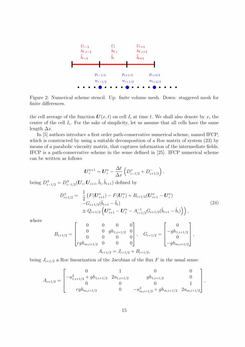
In [5] authors introduce a first order path-conservative numerical scheme, named IFCP,which is constructed by using a suitable decomposition of a Roe matrix of system (23) bymeans of a parabolic viscosity matrix, that captures information of the intermediate fields.IFCP is a path-conservative scheme in the sense defined in [25]. IFCP numerical schemecan be written as follows

Un+1i = Un

i −∆t

∆x

(D+

i−1/2 +D−i+1/2

),

being D±i−1/2 = D±i−1/2(U i,U i+1, bi, bi+1) defined by

D±i+1/2 =1

2

(F (Un

i+1)− F (Uni ) +Bi+1/2(Un

i+1 −Uni )

−Gi+1/2(bi+1 − bi)± Qi+1/2

(Un

i+1 −Uni − A−1

i+1/2Gi+1/2(bi+1 − bi)))

,

(24)

where

Bi+1/2 =

0 0 0 00 0 gh1,i+1/2 00 0 0 0

rghm,i+1/2 0 0 0

, Gi+1/2 =

0

−gh1,i+1/2

0−ghm,i+1/2

,Ai+1/2 = Ji+1/2 +Bi+1/2,

being Ji+1/2 a Roe linearization of the Jacobian of the flux F in the usual sense:

Ai+1/2 =

0 1 0 0

−u21,i+1/2 + gh1,i+1/2 2u1,i+1/2 gh1,i+1/2 0

0 0 0 1rghm,i+1/2 0 −u2

m,i+1/2 + ghm,i+1/2 2um,i+1/2

,

15

and

h∗,i+1/2 =h∗,i + h∗,i+1

2, u∗,i+1/2 =

u∗,i√h∗,i + u∗,i+1

√h∗,i+1√

h∗,i +√h∗,i+1

, ∗ ∈ {1, 2}.

The key point is the definition of the matrix Qi+1/2 ,that in the case of the IFCP is definedby:

Qi+1/2 = α0Id+ α1Ai+1/2 + α2A2i+1/2,

where αj, j = 0, 1, 2 are defined by:1 λ1 λ21

1 λ4 λ24

1 χint χ2int

α0

α1

α2

=

|λ1||λ4||χint|

,where

χint = Sext max(|λ2|, |λ3|),with

Sext =

sgn(λ1 + λ4), if (λ1 + λ4) 6= 0,

1, otherwise.

It can be proved that the numerical scheme is linearly L∞ –stable under the usual CFLcondition.

5.2 Treatment of the non-hydrostatic terms

Regarding non-hydrostatic terms, we consider a staggered-grid (see Figure 2) formed bythe points xi−1/2, xi+1/2 of the interfaces for each cell Ii, and denote the point values ofthe functions p1|b+h2

and w1 on point xi+1/2 at time t by

pi+1/2(t) = p1|b+h2(xi+1/2, t), wi+1/2(t) = w1(xi+1/2, t).

Following [7], p1|b+h2and w1 will be discretized using second order compact finite dif-

ferences. In order to obtain point value approximations for the non-hydrostatic variablespi+1/2 and wi+1/2, operator B(U , ∂xU , b, ∂xb, w1) will be approximated for every pointxi+1/2 of the staggered-grid (Figure (2)). Then, a second order compact finite-differencescheme is applied to

∂tU = T NH(U , ∂xU , b, ∂xb, p1|b+h2, ∂xp1|b+h2

),

∂t(hw1) = p1|b+h2,

B(U , ∂xU , b, ∂xb, w1) = 0,

(25)

where the values obtained in previous step are used as initial condition for the system. Theresulting linear system is solved using an efficient Thomas algorithm.

16

0 5 10 15 20 250.0

0.2

0.4

0.6

0.8

1.0

Free SurfaceBottom

Figure 3: Test 1: Initial condition

6 Numerical tests

In this section we present three numerical tests, for the model proposed in section 4 withthe quadratic friction law proposed in (8). The first one corresponds to the evolution of adune, where the computed velocity of the two-layer model and the one deduced for the SVEmodel are compared. The second test is a dam break problem over an erodible sedimentlayer where laboratory data is used to validate the model. The test proves as well itsvalidity for regions where the interaction between the fluid and the sediment is strong. Inthose situations the velocities computed by the two-layer model and the SVE one are notclose. The last test shows the difference between the hydrostatic and the non-hydrostaticmodel on shape of the bed surface.

The numerical results follow from a combination of the scheme described in Section 5with a discrete approximation of bottom and surface derivatives. The numerical simula-tions are done with a CFL number equal to 0.9.

6.1 Test 1: bedload transport

In this test we would like to show the ability of the proposed model to reproduce thebedload transport. In particular we study the formation and evolution of a dune. To doso, let us consider the following initial condition over a domain of 25m, (see Figure 3):

h2(0, x) =

{0.2 m, if x ∈ [5, 10],0.1 m, otherwise.

h1(0, x) + h2(0, x) = 1 m, q1(0, x) = 1 m2/s2.

The fixed bottom is set to b(x) = 0. We set left boundary condition q1(t, 0) = 1m2/s2, and

17

Figure 4: Test 1: (a) Surface and (b) bottom, at times t = 0, 500, 1000, 1500 s

open boundary condition on the right hand side. The parameters for the model in this aca-demic test have been set as follows: r = 0.34, ds = 0.01m, θc = 0.047, δ = 25o. Ad-ditionally for the transference term we introduce: Ke = 0.1, Kd = 0.01, ϕ = 0.4, n =0.01. We use a discretization of 5000 points for the computational domain.

In Figure 4 we show the free surface and the sediment bottom surface at different times.We can see the dune profile that is transported by the flow.In Figure 5 we show the difference between the velocities um obtained by the model andv

(QF )b , the velocity deduced in [13] for the Saint Venant Exner model given in equation (12).

The difference is of order 10−2 at last computed time t = 1500s. In Figure 6 we show theevolution in time of the relative error between v

(QF )b and um. We remark that it remains

constant in time and the difference is small. The results show that the model behaves wellin low bedload transport regimes and behaves in a similar way as a SVE would.

Figure 5: Test 1: Comparison between um and v(QF )b at time t = 1500 s

18

Figure 6: Test 1: Evolution in time of the relative error between um and v(QF )b in L1, L2

and L∞ norm.

6.2 Test 2: comparison with experimental data

The purpose of this second test is to validate the model with experimental data. This ex-periment has been realized in the laboratory by Spinewine - Zech [31]. The same numericaltest has been performed in [34] using classical models. Nevertheless we remark again thatclassical models make and assumption of low transport regime so that this test is not inthe range of their validity.The experimental test takes place in a rectangular flume, the river bed is flat and at theinitial state, the retained water mass is released. To do so, let us consider the followinginitial condition at the domain [−3 m, 3 m] (see Figure 7):

h1(0, x) =

{10−12 m, if x > 0,0.35 m, if x ≤ 0,

h2(0, x) = 0.05 m, q1(0, x) = q2(0, x) = 0 m2/s2.

The fixed bottom is set to zero and we set open boundary conditions. We choose theparameters given in [34],

r = 0.63, ds = 0.0039 m, θc = 0.047, δ = 35o,

Ke = 0.1, Kd = 0.15, ϕ = 0.4, , n = 0.0039.

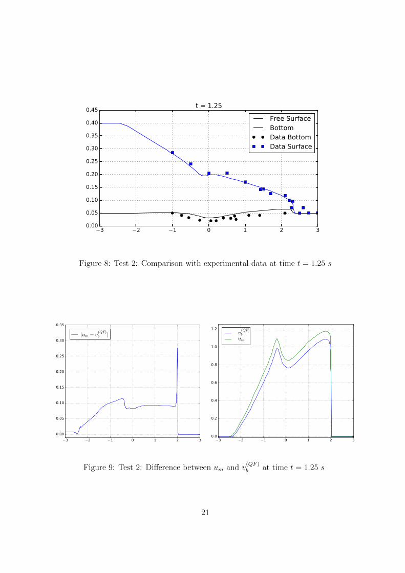
The computational domain used is discretized with 1000 points.In Figure 8 we show the free surface and the sediment bottom surface at time t = 1.25 s

19

Figure 7: Test 2: Initial condition

compared with experimental data. Both free surface and sediment bottom are capturedsuccessfully. Comparing with the results provided in [34] with classical models, we observea better fit to the data for the advancing front of the sediment.As expected, in this test the difference between the velocities um and v

(QF )b is not so small

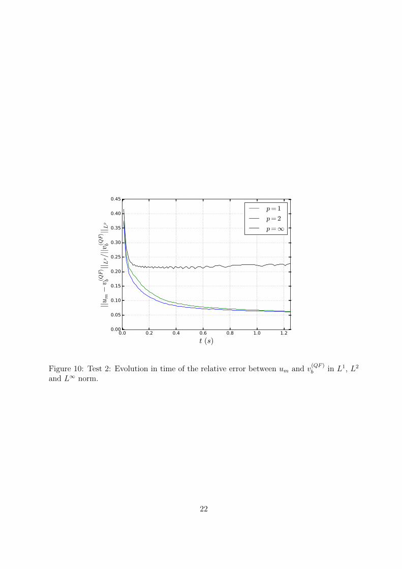
(see Figure 9). Thus, the hypothesis of sediment transport in a small morphodynamic timeis not suitable for this test. In Figure 10 we show the evolution in time of the relative errorbetween v

(QF )b and um. We can observe that the error in norm L∞ remains constant until

the simulated time, where the error in norms L1 and L2 decrease. Nevertheless, duringall the simulation these errors are of a degree of magnitude bigger than for the case ofa dune evolution presented in previous test. The difference is specially relevant at theadvancing front, where the hypothesis of low transport rate is no longer valid. The newmodel introduced here does not requires such assumption.

20

3 2 1 0 1 2 30.00

0.05

0.10

0.15

0.20

0.25

0.30

0.35

0.40

0.45t = 1.25

Free SurfaceBottomData BottomData Surface

Figure 8: Test 2: Comparison with experimental data at time t = 1.25 s

Figure 9: Test 2: Difference between um and v(QF )b at time t = 1.25 s

21

0.0 0.2 0.4 0.6 0.8 1.0 1.2

t (s)

0.00

0.05

0.10

0.15

0.20

0.25

0.30

0.35

0.40

0.45

||um−v

(QF)

b|| L

p/||v

(QF)

b|| L

p

p= 1

p= 2

p=∞

Figure 10: Test 2: Evolution in time of the relative error between um and v(QF )b in L1, L2

and L∞ norm.

22

6.3 Test 3: non-hydrostatic effects

The focus now is to study the influence of the non-hydrostatic effects on the sediment layer,solving the model proposed in section 4. The computational domain is [0 m, 15 m]. Let usconsider the following initial condition

h1(0, x) = 0.8 m h2(0, x) = 0.2 m, q1(0, x) = q2(0, x) = 0 m2/s2.

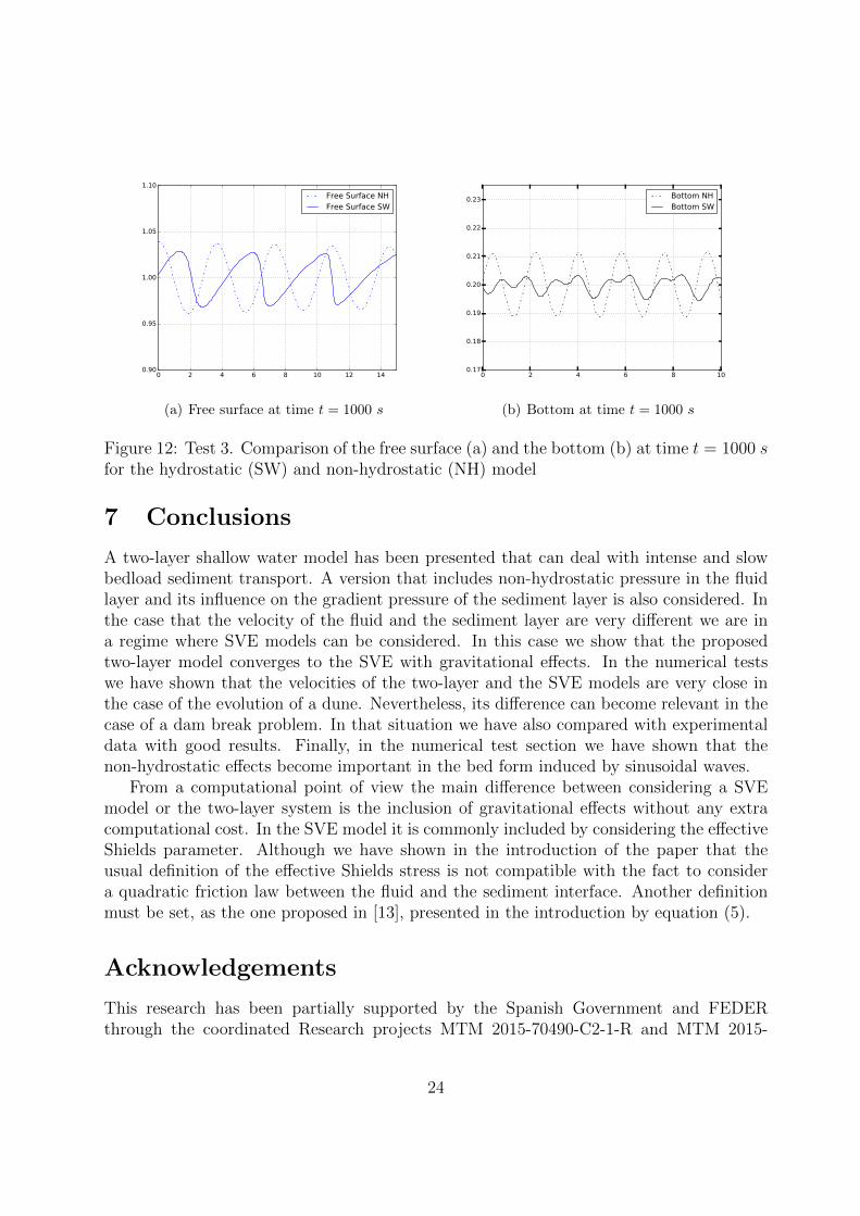
An incoming wave train is simulated through the left boundary condition h1(t, 0) = 0.8 +0.1 sin(5t), and open boundary condition on the right hand side is considered. The param-eters for the model have been set as follows r = 0.63, ds = 0.1, θc = 0.047, δ = 35o,Ke = 0.001, Kd = 0.01, ϕ = 0.4, n = 0.1. We take 1200 points to discretize thedomain.In Figure 11 we show the evolution of the sediment bottom surface at times t = 500, 750, 1000 sfor the model with and without non-hydrostatic effects. A more detailed comparison ofthe final bottom and free surface can be seen in Figure 12. Fredsøe and Deigaard [15]described the behaviour of finite amplitude dunes under a unidirectional current. As it canbe seen, the pattern wave generated by taking into account the non-hydrostatic effects, ismuch more similar to the pattern that can be observed in nature, close to coastal areas.

0 2 4 6 8 10 12 14

0.2

0.4

0.6

0.8

1.0

1.2

Free Surfacet = 500 st = 750 st = 1000 s

Bottomt = 500 st = 750 st = 1000 s

(a) Non-hydrostatic pressure model

0 2 4 6 8 10 12 14

0.2

0.4

0.6

0.8

1.0

1.2

Free Surfacet = 500 st = 750 st = 1000 s

Bottomt = 500 st = 750 st = 1000 s

(b) Hydrostatic pressure model

Figure 11: Test 3. Evolution of the sediment bottom surface at times t =250, 500, 750, 1000 s for the hydrostatic model (6) and non-hydrostatic model (18)-(19)

23

0 2 4 6 8 10 12 140.90

0.95

1.00

1.05

1.10

Free Surface NHFree Surface SW

(a) Free surface at time t = 1000 s

0 2 4 6 8 100.17

0.18

0.19

0.20

0.21

0.22

0.23 Bottom NHBottom SW

(b) Bottom at time t = 1000 s

Figure 12: Test 3. Comparison of the free surface (a) and the bottom (b) at time t = 1000 sfor the hydrostatic (SW) and non-hydrostatic (NH) model

7 Conclusions

A two-layer shallow water model has been presented that can deal with intense and slowbedload sediment transport. A version that includes non-hydrostatic pressure in the fluidlayer and its influence on the gradient pressure of the sediment layer is also considered. Inthe case that the velocity of the fluid and the sediment layer are very different we are ina regime where SVE models can be considered. In this case we show that the proposedtwo-layer model converges to the SVE with gravitational effects. In the numerical testswe have shown that the velocities of the two-layer and the SVE models are very close inthe case of the evolution of a dune. Nevertheless, its difference can become relevant in thecase of a dam break problem. In that situation we have also compared with experimentaldata with good results. Finally, in the numerical test section we have shown that thenon-hydrostatic effects become important in the bed form induced by sinusoidal waves.

From a computational point of view the main difference between considering a SVEmodel or the two-layer system is the inclusion of gravitational effects without any extracomputational cost. In the SVE model it is commonly included by considering the effectiveShields parameter. Although we have shown in the introduction of the paper that theusual definition of the effective Shields stress is not compatible with the fact to considera quadratic friction law between the fluid and the sediment interface. Another definitionmust be set, as the one proposed in [13], presented in the introduction by equation (5).

Acknowledgements

This research has been partially supported by the Spanish Government and FEDERthrough the coordinated Research projects MTM 2015-70490-C2-1-R and MTM 2015-

24

70490-C2-2-R. The authors would like to thank M.J. Castro Dıaz for the fruitful discussionsconcerning non-hydrostatic effects.

References

[1] K. Ashida, M. Michiue. Study on hydraulic resistance and bedload transport rate inalluvial streams. JSCE Tokyo (206): 59–69, 1972.

[2] R.A. Bagnold. The Flow of Cohesionless Grains in Fluids. Royal Society of LondonPhilosophical transactions. Series A. Mathematical and physical sciences, no. 964,1956.

[3] V. Casulli. A semi-implicit finite difference method for non-hydrostatic free surfaceflows, Numerical Methods in Fluids 30 (4), 425–440, 1999.

[4] F. Charru. Selection of the ripple length on a granular bed sheared by a liquid flow.Physics of Fluids (18): 121508, 2006.

[5] E. D. Fernandez-Nieto, M. Castro. C. Pares. On an Intermediate Field CapturingRiemann Solver Based on a Parabolic Viscosity Matrix for the Two-Layer ShallowWater System, J. Sci. Comput. 48(1–3): 117–140, 2011.

[6] H. A. Einstein. Formulas for the transportation of bed load. ASCE. (107): 561–575,1942.

[7] C. Escalante, T. Morales De Luna, M. Castro. Non-hydrostatic pressure shallow flows:GPU implementation using finite-volume and finite-difference scheme. Submitted toApplied Mathematics and Computation, https://arxiv.org/abs/1706.04551, 2017.

[8] F. Engelund, J. Dresoe. A sediment transport model for straight alluvial channels.Nordic Hydrol. (7): 293–306, 1976.

[9] F. Exner, Uber die wechselwirkung zwischen wasser und geschiebe in flussen, Sitzungs-ber., Akad. Wissenschaften pt. IIa. Bd. 134, 1925.

[10] Fernandez Luque & Van Beek. Erosion and transport of bedload sediment. J. Hy-draulaul. Res. (14): 127–144, 1976.

[11] H. Chanson. The hydraulics of open channel flow: an introduction. ElsevierButterworth-Heinemann, Oxford, 2004.

[12] E. D. Fernandez-Nieto, C. Lucas, T. Morales de Luna, S. Cordier. On the influenceof the thickness of the sediment moving layer in the definition of the bedload trasportformula in Exner systems. Comp.& Fluids, 91: 87–106, 2014.

25

[13] E.D. Fernandez-Nieto, T. Morales de Luna, G. Narbona-Reina, J.D. Zabsonre, For-mal deduction of the Saint-Venant-Exner model including arbitrarily sloping sedimentbeds and associated energy, ESAIM: Mathematical Modelling and Numerical Analysis,51:115-145, 2017.

[14] A. C. Fowler, N. Kopteva, and C. Oakley. The formation of river channel. SIAM J.Appl. Math.(67):1016–1040, 2007.

[15] J. Fredsøe, R. Deigaard, Mechanics of Coastal Sediment Transport, World ScientificPublishing Company, ISBN 9810208413, 1992.

[16] G. Garegnani, G. Rosatti, L. Bonaventura. Free surface flows over mobile bed: math-ematical analysis and numerical modeling of coupled and decoupled approaches. Com-munications In Applied And Industrial Mathematics, 2(1), 2011.

[17] M.-O. Bristeau, A. Mangeney, J. Sainte-Marie, N. Seguin, An energy-consistent depth-averaged euler system: Derivation and properties. Discrete and Continuous DynamicalSystems Series B 20 (4), 961–988, 2015.

[18] A. A. Kalinske. Criteria for determining sand transport by surface creep and saltation.Trans. AGU. 23(2): 639–643, 1942.

[19] A. Kovacs, G. Parker. A new vectorial bedload formulation and its application to thetime evolution of straight river channels. J. Fluid Mech., (267):153–183, 1994.

[20] P. Madsen, O. Sørensen, A new form of the boussinesq equations with improved lineardispersion characteristics. part 2: A slowing varying bathymetry, Coastal Engineering18, 183–204, 1992.

[21] Meyer-Peter, R. Muller. Formulas for bedload transport. Rep. 2nd Meet. Int. Assoc.Hydraul. Struct. Res., Stockolm: 39–64, ASCE. (107): 561–575, 1942.

[22] T. Morales de Luna, M. Castro, C. Pares. A duality method for sediment transportbased on a modified Meyer-Peter & Muller model. Journal of Scientific Computing,48(1): 258–273, 2011.

[23] P. Nielsen. Coastal Bottom Boundary Layers and Sediment Transport. World ScientificPublishing, Singapore. Advanced Series on Ocean Engineering, 4, 1992.

[24] G. Parker, G. Seminara, L. Solari. Bed load at low Shields stress on arbitrarilysloping beds: Alternative entrainment formulation. Water Resources Res. (29):7,doi:10.1029/2001WR001253, 2003.

[25] C. Pares, Numerical methods for nonconservative hyperbolic systems: a theoreticalframework. SIAM J. Numer. Anal. 1, 300–321, 2006.

[26] D. Peregrine, Long waves on a beach. Fluid Mechanics 27 (4), 815–827, 1967.

26

[27] S. Soares-Frazao, Dam-break flows over mobile beds: experiments and benchmark testsfor numerical models, Journal of Hydraulic Research, 50(4), 364-375, 2012.

[28] C. Savary, Transcritical transient flow over mobile bed. Two-layer shallow-water model.PhD thesis, Universite catholique de Louvain, 2007.

[29] G. Seminara, L. Solari, G. Parker. Bed load at low Shields stress on arbitrarily slop-ing beds: Failure of the Bagnold hypothesis. Water Resources Res. Vol. 38: 11, doi:10.1029/2001WR000681, 2002.

[30] B. Spinewine, Two-layer flow behaviour and the effects of granular dilatancy in dam-break induced sheet-flow, PhD Thesis n.76, Universite catholique de Louvain, 2005.

[31] B. Spinewine, Y. Zech, Small-scale laboratory dam-break waves on movable beds, J.Hydraulic Res., 45(1), 73-86, 2007.

[32] C. Swartenbroekx, S. Soares-Frazao, B. Spinewine, V. Guinot, Y. Zech, Hyperbolic-ity preserving HLL solver for two-layer shallow-water equations applied to dam-breakflows. River Flow 2010, Dittrich, Koll, Aberle & Geisenhainer (eds.), Bundesanstaltfur Wasserbau (BAW), Karlsruhe, Germany, 2, 1379-1387, 2010.

[33] P. Tassi, S. Rhebergen, C. Vionnet, O. Bokhove. A discontinuous Galerkin finiteelement model for morphodynamical evolution in shallow flows. Comp. Meth. App.Mech. Eng. (197) 2930–2947, 2008.

[34] P. Ung, Simulation numerique du transport sedimentaire. PhD thesis, Universited’Orleans, 2016.

[35] L. C. Van Rijn. Sediment transport (I): bed load transport. J. Hydraul. Div. Proc.ASCE, (110): 1431–56, 1984.

[36] W. Wu, Depth-averaged 2-D numerical modeling of unsteady flow and nonuniformsediment transport in open channels. J. Hydraulic Eng., ASCE, 130(10), 1013-1024,2004.

[37] W. Wu, Computational River Dynamics, Taylor & Francis, UK, 2008.

[38] W. Wu, A depth-averaged 2-d model for coastal levee and barrier island breach pro-cesses. Proc. 2010 World Environmental and Water Resources Congress, Rhode Island(on CD-Rom), 2010.

[39] Y. Yamazaki, Z. Kowalik, K. Cheung, Depth-integrated, non-hydrostatic model forwave breaking and run-up, Numerical Methods in Fluids 61, 473–497, 2008.

27